Quantum annealing showing the exponentially small success probability despite a constant energy gap

Abstract

Quantum annealing (QA) is one of the methods to solve combinatorial optimization problems. We can estimate a computational time of QA by using the so-called adiabatic condition derived from the adiabatic theorem. The adiabatic condition consists of two parts: an energy gap and a transition matrix. It is believed that the computational time mainly depends on the energy gap during QA and is inversely proportional to a polynomial of the minimal energy gap. In this paper, we challenge this common wisdom. We propose a general method to construct counterintuitive models with a constant energy gap during QA where QA with a constant annealing time fails despite a constant energy gap. In our formalism, we choose a known model exhibiting an exponentially small energy gap during QA, and we modify the model by adding a specific penalty term to the Hamiltonian. In the modified model, the transition matrix in the adiabatic condition becomes exponentially large with the number of qubits, while the energy gap remains constant. As concrete examples we consider the adiabatic Grover search and the ferromagnetic $p$-spin model. In these cases, by adding the penalty term, the success probability of QA in the modified models become exponentially small despite a constant energy gap. Our results paves a way for better understanding of the QA performance.

I Introduction

Quantum annealing (QA) is a method to solve combinational optimization problems with quantum properties [1, 2, 3, 4, 5, 6, 7]. The solution of the combinational optimization problems can be embedded in a ground state of a Ising Hamiltonian [8, 9]. On the other hand, the Hamiltonian of the transverse magnetic field is used to induce the quantum fluctuation. We gradually decrease the transverse magnetic field while we gradually increase the Ising Hamiltonian, and we obtain the ground state of the Ising Hamiltonian if the so-called adiabatic condition is satisfied [10, 11, 12, 13, 14, 15]. This condition is given as follows:

$$\frac{|\braket{e(t)}{\partial_{t}{\hat{H}(t)}}{g(t)}|}{\Delta(t)^{2}}\ll 1,$$ (1)

where $H(t)$, $\ket{g}$, $\ket{e}$ and $\Delta$ are a Hamiltonian, a ground state, the first exited state, and an energy gap of these states, respectively. Throughout of this paper, we call the left hand side of Eq. (1) an adiabatic condition term. The energy gap is believed to be related to the computational complexity, and the relationship between them has been studied [16, 17, 18, 19, 20, 21, 22]. Several methods to estimate and control the energy gap have been proposed in order to improve the performance of QA [23, 24, 25, 26, 27, 28].

It is known that a phase transition could occur if there is a competition between the quantum fluctuation and the magnetic interaction. In this case, the energy gap vanishes at the point of the phase transition when the system size goes to an infinity. As is well known in statistical mechanics, the order of systems is characterised by the order parameter. In a second-order phase transition, the order parameter is continuous, whereas in a first-order phase transition, it has discontinuity at a certain time. If the first-order phase transition occurs, it is supposed that the energy gap becomes exponentially small at a phase transition point. When tackling hard problems (that cannot be efficiently solved by classical algorithms) with QA, the first-order phase transition typically occurs. For example, when we solve the exact cover and the database search problem by QA, such a phase transition occurs [29, 30]. As these previous studies show, the performance of QA was believed to be simply determined by the energy gap.

In this paper, we challenge this common wisdom, and propose a systematic method to construct counter-intuitive models where QA with a constant annealing time fails despite a constant energy gap. Actually, not the energy gap but the transition matrix in the adiabatic condition term in Eq. (1) becomes the cause of the failure of QA in our model. (see Table. 1). The key idea of our proposal is to add a penalty term in the Hamiltonian, which does not change the eigenstate of Hamiltonian but change the eigenvalue. By adding such a penalty term, we analytically show that the transition matrix becomes exponentially large while the energy gap remains constant. We also numerically perform QA on the Grover search and the ferromagnetic $p$-spin model. The success probability of QA in these model becomes exponentially small as we increase the problem size $L$ despite an energy gap that scales as $O(L^{0})$ during QA. Therefore, we highlight the importance of the transition matrix, which has been often overlooked in earlier work of QA.

Our paper is organized as follows. In sec. II, we review QA and the adiabatic Grover search. In sec. III, we introduce the general framework to construct the case in which the transition matrix exponentially increases. In sec. IV, as a first example, we applly our general theory to the adiabatic Grover search. In sec. V, as a second example, we perform the numerical analysis in the ferromagnetic $p$-spin model. Finally, sec. VI is devoted to the conclusion.

Table 1: The problem size $L$ (the number of qubit) dependence of the energy gap and the transition matrix in the conventional and our model.

	Energy gap	Transition matrix
	$\Delta(t)$	$\braket{e(t)}{\partial_{t}{\hat{H}(t)}}{g(t)}$
Conventional	exponentially small	${\rm poly}(L)$
Our model	$O(L^{0})$	exponentially large

II Quantum annealing and adiabatic Grover search

Let us review QA and adiabatic Grover search in this section.

II.1 Quantum annealing

In QA, the total Hamiltonian is given as following [4, 5]:

$$H_{QA}(t)=\frac{t}{T}H_{p}+\left(1-\frac{t}{T}\right)H_{d},$$ (2)

where $H_{p}$, $H_{d}$ and $T$ are the problem Hamiltonian, the driver Hamiltonian, and an annealing time, respectively. We prepare a ground state of $H_{d}$, and let this state evolve by the total Hamiltonian. If an initial state at $t=0$ evolves in a sufficiently large $T$ to satisfy the adiabatic condition, we can obtain the ground state of $H_{p}$ at $t=T$. Throughout of our paper, the unit of the Hamiltonian is GHz and time is ns.

II.2 Adiabatic Grover search

Let us consider a problem to search a specific element through a database composed of $N$ elements. On a classical computer, on average, we need to check half of elements to get the target element. Grover proposed the quantum algorithm to search the target element where only $\sqrt{N}$ times of evaluation is required [31]. We can adopt an adiabatic algorithm to search the database, and such an algorithm is called the adiabatic Grover search [4, 32, 7]. In the adiabatic Grover search, the problem Hamiltonian is given by

$$H_{p}=\hat{I}-\ket{m}\bra{m}.$$ (3)

Here, the solution to be found is denoted by $|m\rangle$, and this is represented by the computational basis ($\ket{\uparrow}$ and $\ket{\downarrow}$ ). The number of qubit is $L$, i.e., the dimension of Hilbert space is $2^{L}$. The driver Hamiltonian is described as

$$H_{d}=\hat{I}-\ket{++\cdots+}\bra{++\cdots+},$$ (4)

where $\ket{+}$ is the eigenstate of the Pauli matrix ${\hat{\sigma}_{x}}$, i.e., $\ket{+}=(\ket{\uparrow}+\ket{\downarrow})/\sqrt{2}$. Since the adiabatic Grover search can be block-diagonalized, we can analytically obtain the eingenvalue and eigenstate by diagonalizing a two-by-two matrix. By using the desired state $\ket{m}$ and its orthogonal state $\ket{m^{\perp}}$, the total Hamiltonian $H_{QA}(t)$ can be effectively described as

$$H_{QA}(t)=\frac{1}{2}{\hat{I}}-\frac{\Delta_{0}(t)}{2}{\rm cos\theta}\ \tilde{\sigma^{z}}-\frac{\Delta_{0}(t)}{2}{\rm sin\theta}\ \tilde{\sigma^{x}},$$ (5)

where we define Pauli matrices represented in $\ket{m}$ and $\ket{m^{\perp}}$ basis as $\tilde{\sigma}^{z}\equiv\ket{m}\bra{m}-\ket{m^{\perp}}\bra{m^{\perp}}$ and $\tilde{\sigma}^{x}\equiv\ket{m}\bra{m^{\perp}}+\ket{m^{\perp}}\bra{m}$. Here, ${\rm cos}\theta(t)$, ${\rm sin}\theta(t)$ and $\Delta_{0}(t)$ are given as

$${\rm cos}\theta(t)=\frac{1}{\Delta_{0}(t)}\left[1-2\left(1-t/T\right)(1-2^{-L})\right],$$ (6)

$${\rm sin}\theta(t)=\frac{2}{\Delta_{0}(t)}\left(1-t/T\right)\sqrt{2^{-L}(1-2^{-L})},$$ (7)

$$\Delta_{0}(t)=\sqrt{\left(1-\frac{2t}{T}\right)^{2}+\frac{2^{-L+2}t}{T}\left(1-\frac{t}{T}\right)},$$ (8)

where we choose the branch of ${\rm Tan}^{-1}(x)$ which is given by $-\pi/2\leq{\rm Tan}^{-1}(x)\leq\pi/2$ and we define $\theta(t)={\rm Tan}^{-1}({\rm sin}\theta(t)/{\rm cos}\theta(t))$. The ground state $\ket{g(t)}$ and first excited state $\ket{e(t)}$ of Hamiltonian (5) are given as following:

$$\ket{g(t)}={\rm cos}\frac{\theta(t)}{2}\ket{m}+{\rm sin}\frac{\theta(t)}{2}\ket{m^{\perp}},$$ (9)

$$\ket{e(t)}=-{\rm sin}\frac{\theta(t)}{2}\ket{m}+{\rm cos}\frac{\theta(t)}{2}\ket{m^{\perp}}.$$ (10)

The energy of these states are given by

$$E_{g}(t)=\frac{1}{2}(1-\Delta_{0}(t)),$$ (11)

$$E_{e}(t)=\frac{1}{2}(1+\Delta_{0}(t)).$$ (12)

Thus, the energy gap is $E_{e}(t)-E_{g}(t)=\Delta_{0}(t)$. From Eq. (8), the energy gap scales as $O(2^{-L/2})$ at $t=T/2$. The numerator of the adiabatic condition term (1) for the adiabatic Grover search is $O(L^{0})$ [32]. The annealing time $T$ should scale as $O(2^{L})$ to satisfy the adiabatic condition. This means that the necessary time to find the solution by the adiabatic Grover search is the same as that by a classical search. However, Roland and Cerf showed that the quadratic speed up as well as Grover’s algorithm can be attained by choosing optimal scheduling function [32].

III General Framework

In this section, we show a general method to construct models where QA with a constant annealing time has exponentially small success probability despite a constant energy gap. Suppose we have a system where the transition matrix scales polynomially with $L$ and the energy gap become exponentially small with increasing $L$. Then, we show that, by adding a specific penalty term to the Hamiltonian, we can systematically construct a model with a constant energy gap where the transition matrix becomes exponentially large as the size $L$ increases.

The adiabatic condition term can be written as the following form

$$\eta =\frac{|\braket{e(t)}{\partial_{t}{\hat{H}(t)}}{g(t)}|}{\Delta(t)^{2}}$$

$$=\left[\frac{|\braket{e(t)}{\partial_{t}{\hat{H}(t)}}{g(t)}|}{\Delta(t)}\right]\frac{1}{\Delta(t)}$$ (13)

The squre bracket in the right-hand side of Eq. (III) yields

$$\frac{|\braket{e(t)}{\partial_{t}{\hat{H}(t)}}{g(t)}|}{\Delta(t)}=|\braket{e(t)}{{d}/{dt}}{g(t)}|.$$ (14)

Let us consider the following penalty term (to be added to the Hamiltonian $H_{QA}(t)$)

$$H_{\rm pena}(t)=\sum^{N-1}_{i=0}C_{i}(t)\ket{E_{i}(t)}\bra{E_{i}(t)},$$ (15)

where $N=2^{L}$ denotes the dimension of Hilbert space and $\ket{E_{i}(t)}$ is eigenstate of $H$. The time dependent coefficients $C_{i}(t)$ have a role to shift the eigenenergy of $E_{i}(t)$. In order to keep the energy gap constant during QA, we choose $C_{i}(t)$ as follows:

$$C_{i}(t)=E_{i}(t=0)-E_{i}(t).$$ (16)

From Eq. (14), we show that $\frac{|\braket{e(t)}{\partial_{t}{\hat{H}(t)}}{g(t)}|}{\Delta(t)}$ is unchanged by adding the penalty term to the QA Hamiltonian, because the penalty term is diagonal in the energy eigenstate basis. This means that if we add the penalty term in order to open a exponentially small energy gap, the transition matrix becomes exponentially large. Also, the adiabatic condition term becomes larger by a factor of $1/\Delta(t)$, and so we achieve a speedup of $\Delta(t)$ by adding the penalty term.

For example, let us consider a QA model where the scaling of $|\braket{e(t)}{\partial_{t}{\hat{H}(t)}}{g(t)}|$ ($\Delta(t)$) is given as $O(L^{0})$ ($O(2^{-L/2})$). In this case, as will be shown later, by adding the penalty term (15), we change the energy gap $\Delta(t)$ from $O(2^{-L/2})$ to $O(L^{0})$ while we change the transition matrix $|\braket{e(t)}{\partial_{t}{\hat{H}(t)}}{g(t)}|$ from $O(L^{0})$ to $O(2^{L/2})$. Thus, we achieve a speedup of $2^{-L/2}$.

IV adiabatic Grover search with penalty term

In the first example, we apply our theory to the adiabatic Grover search . Actually, we show that transition matrix becomes exponentially large in the adiabatic Grover search with the penalty term (15). In this section, first, we analytically investigate the scaling of the adiabatic condition term in this model. Subsequently, we numerically show that the success probability of QA becomes exponentially small.

IV.1 Scaling of adiabatic condition term

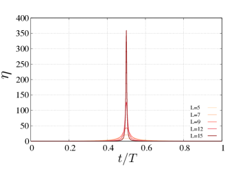
Figure 1: Plot of the adiabatic condition term $\eta$ for the adiabatic Grover search as a function of normalized time $t/T$, where $L$ is the number of qubit.

We consider the Hamiltonian (5), and the penalty term is given by

$$H_{\rm pena}(t)=-E_{g}(t)\ket{g(t)}\bra{g(t)}+\{1-E_{e}(t)\}\ket{e(t)}\bra{e(t)},$$ (17)

where we use Eq. (9) and (10). Also, the total Hamiltonian is written as follows

$$H(t) =H_{QA}(t)+H_{\rm pena}(t)$$

$$=\frac{1}{2}{\hat{I}}-\frac{1}{2}{\rm cos}\theta(t)\ \tilde{\sigma}^{z}-\frac{1}{2}{\rm sin}\theta(t)\ \tilde{\sigma}^{x}.$$ (18)

We can calculate the energy of the ground state $E^{\prime}_{g}(t)$ (first excited state $E^{\prime}_{e}(t)$) as $E^{\prime}_{g}(t)=0$ ($E^{\prime}_{e}(t)=1$) in the model (18). Since we have $E^{\prime}_{e}(t)-E^{\prime}_{g}(t)=1$, the energy gap of our model does not depend on the number of qubit $L$. Fig. 1 show the adiabatic condition term as function of $t$. At $t=T/2$, the adiabatic condition term becomes exponentially larger as increasing $L$. Let us analyze the scaling of the adiabatic condition term. From Eqs. (9), (10) and (14), we obtain

$$|\braket{e(t)}{d/dt}{g(t)}|=\frac{\sqrt{(1-2^{-L})2^{-L}}}{T(1+4\left(\frac{t}{T}\right)^{2}(1-2^{-L})-4\frac{t}{T}(1-2^{-L}))}.$$ (19)

at $t=T/2$, Eq. (19) yields

$$|\braket{e(t)}{d/dt}{g(t)}|=\frac{1}{T}\sqrt{2^{L}-1}\sim O(2^{L/2}).$$ (20)

Since the energy gap is always constant due to the penalty term, the scaling of the adiabatic condition term is $\eta\sim$ $O(2^{L/2})$ at $t=T/2$. This indicates that the adiabatic condition term is improved by the factor of $\Delta_{0}^{-1}$ compared to the case without the penalty term. From Eq. (14) and (20), the transition matrix becomes

$$\braket{e(t)}{\partial_{t}H(t)}{g(t)}\sim O(2^{L/2}).$$ (21)

Hence, as we expected from our general framework, the divergence of the adiabatic condition term in Fig. 1 stems from the exponentially large transition matrix (21).

As is well known, quantum many-body systems often have the point of a gap closing due to the quantum phase transition [34, 35, 36, 16]. In the adiabatic Grover search, also, the competition of the driver Hamiltonian and the problem Hamiltonian cause the first-order quantum phase transition from the paramagnetic phase to the ferromagnetic phase. The energy gap at this phase transition point becomes exponentially small as we increase the size $L$ and vanishes in the thermodynamic limit $L\rightarrow\infty$. On the other hand, the energy gap in our model with the penalty term does not close in the thermodynamic limit, which seems to avoid the first-order phase transition by adding the penalty term. To check whether the first-order phase transition exists, we analyze the total magnetization as the order parameter. This analysis is essentially equivalent to the mean field analysis of a $p$-spin model for $p\rightarrow\infty$[36]. On the other hand, we directly obtain the magnetization by using the ground state of our model (IV.1) unlike Ref. [36]. The total magnetization of the ground state is given by

$$\braket{g(t)}{\sum_{i}^{L}{\hat{\sigma}^{z}_{i}}}{g(t)}={\rm cos}^{2}\frac{\theta(t)}{2}-\frac{1}{2^{L}-1}{\rm sin}^{2}\frac{\theta(t)}{2},$$ (22)

where ${\hat{\sigma}}^{z}$ is a $z$ component of the Pauli matrix, ${\hat{\sigma}}^{z}=\ket{\uparrow}\bra{\uparrow}-\ket{\downarrow}\bra{\downarrow}$. The existence of the first-order phase transition can be shown as the discontinuity of magnetization at $t=T/2$ in the thermodynamic limit. We take the thermodynamic limit as $L\rightarrow\infty$ for Eq. (22),

$$\lim_{L\to\infty}\left({\rm cos}^{2}\frac{\theta(t)}{2}-\frac{1}{2^{L}-1}{\rm sin}^{2}\frac{\theta(t)}{2}\right) =\frac{1}{2}+\frac{1}{2}\lim_{L\to\infty}{\rm cos}\theta(t)$$

$$=\frac{1}{2}-\frac{1-2(t/T)}{2|1-2(t/T)|}.$$ (23)

Thus, we obtain

$$\lim_{t\to\frac{T}{2}-0}\lim_{L\to\infty}\braket{g(t)}{\sum_{i}^{L}{\hat{\sigma}^{z}_{i}}}{g(t)}=0,$$ (24)

$$\lim_{t\to\frac{T}{2}+0}\lim_{L\to\infty}\braket{g(t)}{\sum_{i}^{L}{\hat{\sigma}^{z}_{i}}}{g(t)}=1.$$ (25)

Therefore, in our model, the first-order phase transition occurs at $t=T/2$ even if the gap is $O(L^{0})$.

IV.2 Numerical analysis

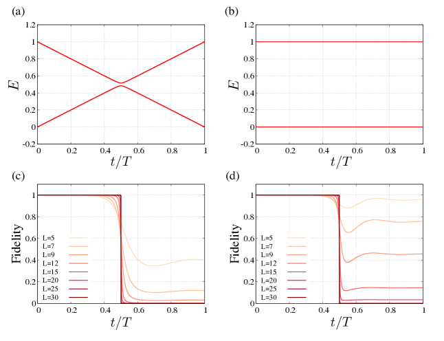
Figure 2: The energy spectrum and the fidelity for the adiabatic Grover search as the function of $t/T$. The energy diagram in $L=10$ (a) without the penalty term and (b) with the penalty term. The fidelity (c) without the penalty term and (d) with the penalty term. We set the annealing time $T=20$.

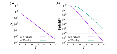
Figure 3: The scaling of (a) the energy gap at $t=T/2$ and (b) the fidelity at $t=T$ for the adiabatic Grover search. The purple line and the green line correspond to the case without and with the penalty term, respectively. We set the annealing time $T=20$.

To investigate the effect of the exponential increase of the transition matrix on QA, we perform numerical calculations. Fig. 2(a) and (b) show the energy spectrum. In the case without the penalty term, the energy gap becomes minimum at $t=T/2$. On the other hand, in the case with the penalty term, the energy gap is constant and does not depend on the number of qubit $L$ as shown in Fig. 3 (a). We numerically solve the Schrödinger equation, and obtain a state $\ket{\Psi_{0}(t)}$. We show the fidelity as the function of $t$ in Fig. 2(c) and (d) where we define the fidelity as $|\braket{\Psi_{0}(t)}{g(t)}|^{2}$. As $L$ increases, the fidelity decrease more rapidly around $t=T/2$ due to the non-adiabatic transition to the first excited state.

Fig. 3 (a) and (b) show the scaling of the energy gap at $t=T/2$ and the fidelity at $t=T$. In the case without the penalty term, the energy gap becomes exponentially small. As mentioned in the section II, the scaling of transition matrix is $O(L^{0})$ for the case without the penalty term. Therefore, the exponential decrease of the fidelity (the purple line in Fig. 3(b)) is originated from the gap closing at $t=T/2$. On the other hand, in the case with penalty term, the energy gap does not depend on $L$. Thus, the decrease of the fidelity (the green line in Fig. 3(b)) is originated from the exponential increase of transition matrix. We note that, in Fig. 3 (b), the fidelity with the penalty term is larger than that without the penalty term. This behavior is consistent with our general framework to show that the adiabatic condition term with the penalty term is smaller than that without the penalty term.

V Ferromagnetic $p$ spin model

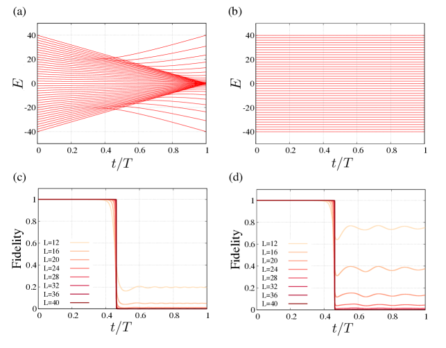
Figure 4: The energy spectrum and the fidelity as the function of $t/T$ for the ferromagnetic $p$-spin model. The energy diagram in $L=40$ (a) without the penalty term and (b) with the penalty term. The fidelity (c) without the penalty term and (d) with the penalty term. We set the annealing time $T=20$ and also set $p=5$.

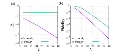
Figure 5: (a) The minimum of the energy gap and (b) the scaling of the fidelity at $t=T$ for the ferromagnetic $p$-spin model. The purple line and the green line denote without and with penalty term, respectively. We set the annealing time $T=20$ and also set $p=5$.

As a second example, we apply our theory to the ferromagnetic $p$-spin model [36, 16, 37]. The problem Hamiltonian is given by

$$H_{p}=-L\left(\frac{1}{L}\sum^{L}_{i=1}\hat{\sigma}^{z}_{i}\right)^{p}.$$ (26)

We use the transverse field as the driver Hamiltonian given as $H_{d}=-\sum^{L}_{i}\hat{\sigma}^{x}_{i=1}$. The Hamiltonian of QA is given as follow:

$$H_{QA}(t)=\frac{t}{T}H_{p}+\left(1-\frac{t}{T}\right)H_{d}.$$ (27)

The penalty term is given as

$$H_{\rm pena}(t)=\sum_{i=0}^{2S}\{E_{i}({t=0})-E_{i}(t)\}\ket{E_{i}(t)}\bra{E_{i}(t)},$$ (28)

where $S$ is the maximum angular momentum and $\ket{E_{i}}$ ($E_{i}$) is the eigenstate (eigenenergy) of $H_{QA}(t)$. We numerically diagonalize $H_{QA}(t)$ at each time and construct the penalty term. The total Hamiltonian is given as

$$H(t)=H_{QA}(t)+H_{\rm pena}(t).$$ (29)

The component of the total spin operator can be represented as following: $\hat{S}^{z}=\sum^{L}_{i=1}\hat{\sigma}^{z}_{i}/2$ and $\hat{S}^{x}=\sum^{L}_{i=1}\hat{\sigma}^{x}_{i}/2$. As the total spin operator $\hat{\bm{S}}$ is conserved, we consider only the subspace of $2S=L$.

The ferromagnetic $p$-spin model with transverse field for $p=2$ ($p\geq 3$) has the second-order (first-order) phase transition point in QA [36, 16, 37]. Throughout of our paper, we set $p=5$. Fig. 4 (a) and (b) show the energy spectrum of $L=40$. The minimum of the energy gap is at $t/T\sim 0.463$ (Figure 4(a)). We numerically solve the Schrödinger equation, and plot the fidelity without and with the penalty term, in Fig. 4(c) and (d), respectively. As shown in Fig. 4(b), the energy gap is always constant in the case with penalty term. At $t/T\sim 0.463$, however, the fidelity rapidly decrease as we increase the number of qubit (Fig. 4(d)). We plot the scaling of the minimum energy gap and plot the fidelity at $t=T$ in Fig. 5(a) and (b), respectively. As clearly seen, these results are consistent with our general framework’s prediction, i.e., despite constant energy gap, the fidelity exponentially decays due to the exponential increase of the transition matrix in the case with the penalty term. In addition, the decrease of the fidelity with the penalty term is alleviated compared to that without the penalty term.

VI Conclusion

In conclusion, we propose a general method to construct models where QA with a constant annealing time fails despite a constant energy gap. In our framework, we choose a known model showing an exponentially small energy gap during QA, and add a penalty term to the Hamiltonian. In the modified model, a transition matrix in the adiabatic condition term becomes exponentially larger as the number of qubits increases, while the energy gap is constant.

Based on our framework, we investigated two models as concrete examples: the adiabatic Grover search and the ferromagnetic $p$-spin model. In the adiabatic Grover search, we analytically showed that the transition matrix becomes exponentially large and the magnetization has discontinuity, i.e. first-order phase transition occurs although the energy gap is always constant in QA. Moreover, in the adiabatic Grover search and the ferromagnetic $p$-spin model, we numerically showed that the success probability exponentially decay due to the exponential increase of the transition matrix. Since it is believed that the computational speed in QA is limited by an energy gap that corresponds to the denominator of the adiabatic condition term, our results challenge the common wisdom and will lead to a deeper understanding of the QA performance.