Distributional Robustness Bounds Generalization Errors

Abstract

Bayesian methods, distributionally robust optimization methods, and regularization methods are three pillars of trustworthy machine learning hedging against distributional uncertainty, e.g., the uncertainty of an empirical distribution compared to the true underlying distribution. This paper investigates the connections among the three frameworks and, in particular, explores why these frameworks tend to have smaller generalization errors. Specifically, first, we suggest a quantitative definition for “distributional robustness”, propose the concept of “robustness measure”, and formalize several philosophical concepts in distributionally robust optimization. Second, we show that Bayesian methods are distributionally robust in the probably approximately correct (PAC) sense; In addition, by constructing a Dirichlet-process-like prior in Bayesian nonparametrics, it can be proven that any regularized empirical risk minimization method is equivalent to a Bayesian method. Third, we show that generalization errors of machine learning models can be characterized using the distributional uncertainty of the nominal distribution and the robustness measures of these machine learning models, which is a new perspective to bound generalization errors, and therefore, explain the reason why distributionally robust machine learning models, Bayesian models, and regularization models tend to have smaller generalization errors.

Keywords: Statistical Machine Learning, Generalization Error, Distributionally Robust Optimization, Bayesian Nonparametrics, Regularization Method.

1 Introduction

1.1 Background

A great number of supervised machine learning problems can be modeled by the optimization problem

$$\min_{\bm{x}\in\mathcal{X}}~{}\mathbb{E}_{\mathbb{P}_{0}}h(\bm{x},\mathbf{\xi}),$$ (1)

where $\bm{x}$ is the decision vector, $\mathcal{X}\subseteq\mathbb{R}^{l}$ is the feasible region, and $\mathbf{\xi}$ is the parameter supported on $\Xi\subseteq\mathbb{R}^{m}$; the parameter $\mathbf{\xi}$ is a random vector and $\mathbb{P}_{0}$ is its true underlying distribution; $h:\mathcal{X}\times\Xi\to\mathbb{R}$ (typically $\mathbb{R}_{+}$) is the cost function. For example, see Vapnik (2000, Chap. 1.2), Bishop and Nasrabadi (2006, Chap. 1.5), James et al. (2021, Chap. 2.1), Kuhn et al. (2019). To be specific, in data-driven machine learning, $\mathbf{\xi}$ can represent a data pair $({\bm{X}},{\bm{Y}})$, i.e., $\mathbf{\xi}\coloneqq({\bm{X}},{\bm{Y}})$, where ${\bm{X}}$ is the feature vector and ${\bm{Y}}$ is the response, $\bm{x}$ is the parameter of the hypothesis which is a function from ${\bm{X}}$ to ${\bm{Y}}$.

The optimization problem (1) is also popular in several other areas than machine learning where the specific meanings that it conveys vary from one to another. Non-exhaustive examples are as follows.

1. In applied statistics, (1) can be an M-estimation model where $h$ is termed a random criterion function and $\bm{x}$ is usually the parameter of the distribution $\mathbb{P}_{0}$ such as the location parameter (Huber, 1964; Huber and Ronchetti, 2009), (Van der Vaart, 2000, Chap. 5). The parameter $\bm{x}$ is unknown and to be estimated from $n$ i.i.d. observations $\{\xi_{i}\}_{i\in[n]}$.

2. In operations research and management science, (1) is a stochastic programming model (Shapiro et al., 2009; Anderson and Nguyen, 2020), where $h$ is the cost function such as mean(-variance) objective (Blanchet et al., 2021; Gotoh et al., 2021) and value-at-risk (VaR) objective (Shapiro et al., 2009, p. 16); VaR can be reformulated to the form of (1). Typical examples include the portfolio selection problem and the inventory control problem (Shapiro et al., 2009). Specifically, taking the one-stage inventory control problem as an example, $\mathbf{\xi}$ represents the random demand and $\bm{x}$ is the optimal ordering quantity.

3. In statistical signal processing, (1) can be a state estimation model (Anderson and Moore, 1979, Chap. 2), (Hassibi et al., 1996, Eq. (6)), (Wang, 2022b, pp. 111), in which the unobservable state is to be estimated from the observable measurements. Specifically, $\mathbf{\xi}\coloneqq({\bm{X}},{\bm{Y}})$ where ${\bm{X}}$ is the state vector and ${\bm{Y}}$ is the measurement vector; $\bm{x}$ is the parameter of a state estimator which is a function from ${\bm{Y}}$ to ${\bm{X}}$. State estimation problems are also popular in the machine learning community, for example, inference problems for a hidden Markov process (from observable variables ${\bm{Y}}$ to hidden variables ${\bm{X}}$); see, e.g., Bishop and Nasrabadi (2006, Chap. 13).

When the true underlying distribution $\mathbb{P}_{0}$ is unknown, it can be estimated from observations $\{\xi_{i}\}_{i\in[n]}$ (usually i.i.d.) and this class of problems is termed data-driven problems in the literature (Kuhn et al., 2019). Most applied statistics problems, operations research problems, and supervised machine learning problems belong to this category. The distribution $\mathbb{P}_{0}$ may alternatively be obtained from physics (e.g., from a hidden Morkov process model) and we term this type of problem as model-driven problems in this paper. Most signal processing problems (e.g., state estimation problems) and engineering automatic control problems (Van Parys et al., 2015), among many others, are members of this class.

In this paper, we collectively refer to the two cases as machine learning problems and distinguish them as data-driven machine learning problems and model-driven machine learning problems. This is because the two kinds of problems share the same philosophy that a proportion of data is used to predict the rest by leveraging the distribution $\mathbb{P}_{0}$ (or an estimate of $\mathbb{P}_{0}$). For example, in the data-driven setting, the feature data ${\bm{X}}$ can be used to produce the predicted response $\hat{{\bm{Y}}}$ such that the predicted response $\hat{{\bm{Y}}}$ is close to the true response ${\bm{Y}}$. For another example, in the model-driven setting, the measurement ${\bm{Y}}$ can be used to produce the estimated state $\hat{{\bm{X}}}$ such that the estimated state $\hat{{\bm{X}}}$ is close to the true state ${\bm{X}}$. However, a model-driven problem can be transformed into a data-driven counterpart if the integral $\mathbb{E}_{\mathbb{P}_{0}}h(\bm{x},\mathbf{\xi})$ is hard to be analytically evaluated, and therefore, a Monte–Carlo sampling technique (e.g., importance sampling) is used to simulate data from $\mathbb{P}_{0}$ and then approximate the integral by a $n$-sample weighted sum $\sum^{n}_{i=1}\mu_{i}h(\bm{x},\mathbf{\xi}_{i})$ (Bishop and Nasrabadi, 2006, Chap. 11), where $\mathbb{P}_{0}$ is approximated by a discrete distribution $\sum^{n}_{i=1}\mu_{i}\delta_{\mathbf{\xi}_{i}}$ and $\delta_{\mathbf{\xi}_{i}}$ is the Dirac measure at $\mathbf{\xi}_{i}$; $\mu_{i}$ is the weight of the sample $\mathbf{\xi}_{i}$. An excellent example of using Monte–Carlo sampling to transform a model-driven problem to a data-driven counterpart is the particle filter for state estimation of a hidden Markov model (Bishop and Nasrabadi, 2006, Chap. 13.3.4), (Wang, 2022a). Hence, without the loss of practical generality, it is sufficient to investigate only the data-driven case.

1.2 Problem Statement

In both the data-driven setting and the model-driven setting, the nominal distribution $\bar{\mathbb{P}}$, which is an estimate of the true distribution $\mathbb{P}_{0}$, might be uncertain: There might be a discrepancy between $\bar{\mathbb{P}}$ and $\mathbb{P}_{0}$. To be specific, in the data-driven setting, the uncertainty of the empirical distribution $\hat{\mathbb{P}}_{n}$ (i.e., $\bar{\mathbb{P}}\coloneqq\hat{\mathbb{P}}_{n}$) might be due to scarce data, while in the model-driven setting the uncertainty might be due to the inexact modeling of physical laws or to the incorrect model assumptions. Usually, neglecting such distributional uncertainty in $\bar{\mathbb{P}}$ and directly using the nominal model

$$\min_{\bm{x}\in\mathcal{X}}\mathbb{E}_{\bar{\mathbb{P}}}h(\bm{x},\mathbf{\xi})$$ (2)

as a surrogate for the true model (1), i.e., $\min_{\bm{x}}\mathbb{E}_{\mathbb{P}_{0}}h(\bm{x},\mathbf{\xi})$, may cause significant performance degradation; i.e., $\mathbb{E}_{\mathbb{P}_{0}}h(\bar{\bm{x}},\mathbf{\xi})$ may significantly excess $\min_{\bm{x}}\mathbb{E}_{\mathbb{P}_{0}}h(\bm{x},\mathbf{\xi})$ where $\bar{\bm{x}}\in\operatorname*{argmin}_{\bm{x}}\mathbb{E}_{\bar{\mathbb{P}}}h(\bm{x},\mathbf{\xi})$. Therefore, reducing the negative influence caused by the distributional uncertainty in $\bar{\mathbb{P}}$ is the core of trustworthy machine learning. In other words, the expected generalization error, i.e.,

$$\mathbb{E}\left[\mathbb{E}_{\mathbb{P}_{0}}h(\bar{\bm{x}},\mathbf{\xi})-\mathbb{E}_{\bar{\mathbb{P}}}h(\bar{\bm{x}},\mathbf{\xi})\right]$$ (3)

of a machine learning model working with $\bar{\mathbb{P}}$ should be controlled, where the outer expectation is taken with respect to the randomness in $\bar{\mathbb{P}}$. Note that $\bar{\mathbb{P}}$ might be a random measure such as the empirical measure $\hat{\mathbb{P}}_{n}$. For example, in the data-driven setting, (3) is particularized to

$$\mathbb{E}_{\mathbb{P}^{n}_{0}}\left[\mathbb{E}_{\mathbb{P}_{0}}h(\hat{\bm{x}}_{n},\mathbf{\xi})-\mathbb{E}_{\hat{\mathbb{P}}_{n}}h(\hat{\bm{x}}_{n},\mathbf{\xi})\right],$$ (4)

which is the typical definition of the expected generalization error of the machine learning model $\min_{\bm{x}}\mathbb{E}_{\hat{\mathbb{P}}_{n}}h(\bm{x},\mathbf{\xi})$, where $\mathbb{P}^{n}_{0}$ is the $n$-fold product measure induced by $\mathbb{P}_{0}$ and $\hat{\bm{x}}_{n}\in\operatorname*{argmin}_{\bm{x}}\mathbb{E}_{\hat{\mathbb{P}}_{n}}h(\bm{x},\mathbf{\xi})$.

Trustworthy machine learning hence aims to design a new model based on, instead of directly using, the nominal/surrogate model (2) such that the expected generalization error (3) is minimized or controlled.

1.3 Literature Review

Facing the distributional mismatch between $\bar{\mathbb{P}}$ and $\mathbb{P}_{0}$, Bayesian methods are the earliest and also the first-hand choice (Ferguson, 1973; Ghosal and Van der Vaart, 2017; Wu et al., 2018). Suppose we can construct a family $\mathcal{C}\subseteq\mathcal{M}(\Xi)$ of nominal distributions based on the knowledge of $\bar{\mathbb{P}}$ where $\mathcal{M}(\Xi)$ is the set of all distributions on the measurable space $(\Xi,\mathcal{B}_{\Xi})$ and $\mathcal{B}_{\Xi}$ is the Borel $\sigma$-algebra on $\Xi$. For example, $\mathcal{C}$ can be a closed distributional $\epsilon$-ball centered at $\bar{\mathbb{P}}$, i.e., $\mathcal{C}\coloneqq B_{\epsilon}(\bar{\mathbb{P}})$. Bayesian methods try to assign a distribution $\mathbb{Q}$ on the measurable space $(\mathcal{C},\mathcal{B}_{\mathcal{C}})$ and solve the Bayesian counterpart of the nominal model (2):

$$\min_{\bm{x}\in\mathcal{X}}\mathbb{E}_{\mathbb{Q}}\mathbb{E}_{\mathbb{P}}h(\bm{x},\mathbf{\xi}),$$ (5)

where $\mathbb{P}\in\mathcal{C}$ and $\mathbb{Q}\in\mathcal{M}(\mathcal{C})$; i.e., $\mathbb{P}\sim\mathbb{Q}$. (Note that $\mathbb{P}$ and $\mathbb{Q}$ may be non-parametric.) In this case, we need to guarantee that $\mathbb{P}_{0}\in\mathcal{C}$ and $\mathbb{Q}$ should be such that $\mathbb{P}_{0}$ is the element that is most probable to be drawn from $\mathcal{C}$. In fact, under some mild conditions, there exists an element $\mathbb{P}^{\prime}\in\mathcal{C}$ such that $\mathbb{E}_{\mathbb{Q}}\mathbb{E}_{\mathbb{P}}h(\bm{x},\mathbf{\xi})=\mathbb{E}_{\mathbb{P}^{\prime}}h(\bm{x},\mathbf{\xi})$ for every $\bm{x}$; see Theorem 18. Therefore, in nature, Bayesian methods inform us of a possible way to choose the “best” candidate $\mathbb{P}^{\prime}$ from the nominal distribution class $\mathcal{C}$. The ideal case is that $\mathbb{P}^{\prime}$ can coincide with $\mathbb{P}_{0}$. If $\mathbb{P}^{\prime}$ is a better surrogate for (i.e., is closer to) $\mathbb{P}_{0}$ than $\bar{\mathbb{P}}$, Bayesian methods are potential to reduce generalization errors.

Another promising and popular treatment gives rise of the min-max distributionally robust optimization (DRO) framework (Rahimian and Mehrotra, 2022)

$$\min_{\bm{x}\in\mathcal{X}}\max_{\mathbb{P}\in\mathcal{C}}\mathbb{E}_{\mathbb{P}}h(\bm{x},\mathbf{\xi}),$$ (6)

if we are interested in controlling the worst-case performance of the nominal model (2). When the underlying true distribution $\mathbb{P}_{0}$ is contained in $\mathcal{C}$, by minimizing the worst-case cost, the cost at $\mathbb{P}_{0}$ can be also expected to be put down; For more justifications on DRO methods, see Kuhn et al. (2019). Under some mild conditions, there exists a distribution $\mathbb{P}^{\prime}$ such that $\min_{\bm{x}\in\mathcal{X}}\max_{\mathbb{P}\in\mathcal{C}}\mathbb{E}_{\mathbb{P}}h(\bm{x},\mathbf{\xi})=\min_{\bm{x}\in\mathcal{X}}\mathbb{E}_{\mathbb{P}^{\prime}}h(\bm{x},\mathbf{\xi})$ (Mohajerin Esfahani and Kuhn, 2018; Yue et al., 2021; Zhang et al., 2022; Gao, 2022; Gao and Kleywegt, 2022). Hence, in nature, DRO methods advise us of another way to find the “best” candidate $\mathbb{P}^{\prime}$ from the nominal distribution class $\mathcal{C}$. However, the diameter of $\mathcal{C}$, e.g., the radius $\epsilon$ of the associated distributional ball $B_{\epsilon}(\bar{\mathbb{P}})=:\mathcal{C}$, needs to be elegantly specified: neither too small nor too large. If the diameter is too small, $\mathbb{P}_{0}$ may not be included in $\mathcal{C}$, and as a result, the true optimal cost $\min_{\bm{x}}\mathbb{E}_{\mathbb{P}_{0}}h(\bm{x},\mathbf{\xi})$ cannot be upper bounded by the worst-case cost (6). If, on the other hand, the diameter of $\mathcal{C}$ is extremely large, the DRO method may be overly conservative: The upper bound (6) may be too loose, far upward away from the true optimal cost $\min_{\bm{x}}\mathbb{E}_{\mathbb{P}_{0}}h(\bm{x},\mathbf{\xi})$. Interested readers may refer to, e.g., Mohajerin Esfahani and Kuhn (2018); Shapiro (2017); Sun and Xu (2016); Gao and Kleywegt (2022); Gao (2022) for more technical discussions on the DRO method. A comprehensive survey (Rahimian and Mehrotra, 2022) is also recommended for the general information of the DRO method.

Yet another strategy to hedge against the distributional uncertainty in $\bar{\mathbb{P}}$ is to use a regularizer $f(\bm{x})$, that is, to solve the regularized problem (Vapnik, 1998, Chap. A1.3) of the nominal model (2):

$$\min_{\bm{x}\in\mathcal{X}}\mathbb{E}_{\bar{\mathbb{P}}}h(\bm{x},\mathbf{\xi})+\lambda f(\bm{x}),$$ (7)

where $\lambda\geq 0$ is a weight coefficient. This is a trending method in data-driven machine learning and applied statistics to reduce “over-fitting”. A well-known instance is the regularized empirical risk minimization model $\min_{\bm{x}\in\mathcal{X}}\mathbb{E}_{\hat{\mathbb{P}}_{n}}h(\bm{x},\mathbf{\xi})+\lambda_{n}f(\bm{x})$ where $\bar{\mathbb{P}}\coloneqq\hat{\mathbb{P}}_{n}$ is the empirical distribution given $n$ i.i.d. samples, $f(\bm{x})$ is the regularization term (e.g., any norm $\|\bm{x}\|$ of $\bm{x}$; see, e.g., Goodfellow et al. (2016, Chap. 7)), and the weight coefficient $\lambda_{n}$ may depend on $n$. By introducing a bias term $f(\bm{x})$, the generalization errors of the model (7) are possible to be reduced; Recall the “bias-variance trade-off” in machine learning (Hastie et al., 2009, Chap. 2.9), (Domingos, 2012).

When we focus on the data-driven version of (2), that is, $\mathbb{P}_{0}$ is unknown but we have access to $n$ i.i.d. samples $\{\mathbf{\xi}_{i}\}_{i\in[n]}$, (2) is particularized into

$$\min_{\bm{x}\in\mathcal{X}}\mathbb{E}_{\hat{\mathbb{P}}_{n}}h(\bm{x},\mathbf{\xi}),$$ (8)

which is a sample-average approximation (SAA) model known in the operations research community (Anderson and Nguyen, 2020) or an empirical risk minimization (ERM) model known in the machine learning community (Murphy, 2012; Mohri et al., 2018). In this paper, we interchangeably use the two terms SAA and ERM. The generalization performance of ERM is unsatisfactory due to the over-fitting issue on limited data samples. Bayesian methods are potential in reducing the generalization errors (Wu et al., 2018; Anderson and Nguyen, 2020). Regularized SAA methods are also popular to combat over-fitting and reduce the generalization errors (Goodfellow et al., 2016; Shafieezadeh-Abadeh et al., 2019; Germain et al., 2016). The DRO methods can provide a generalization error bound that is independent of the complexity of the hypothesis class (e.g., Vapnik–Chervonenkis dimension, Rademacher complexity) and even applicable for hypothesis classes that have infinite Vapnik–Chervonenkis (VC) dimensions (Shafieezadeh-Abadeh et al., 2019). An exciting property of the DRO method is that, under some conditions, it is equivalent to a regularized empirical risk minimization method (Shafieezadeh-Abadeh et al., 2019; Gao et al., 2022), (Mohajerin Esfahani and Kuhn, 2018, Thm. 6.3), (Kuhn et al., 2019, Thm. 10), (Chen et al., 2020, Chap. 4), which explains why the DRO method can generalize well.

1.4 Research Gaps and Motivations

The terminology “distributional robustness”, although widely used, is just a philosophical concept that has not been quantitatively defined. In other words, there does not exist a quantity to measure the distributional robustness of a “robust solution”. Therefore, the first motivation of this work is to formalize the DRO theory and explain the rationale and limitation of the existing min-max DRO model (6).

Although Bayesian probabilistic interpretation for some special regularized methods (specifically, LASSO and Ridge regression) exists and recent results show that there is a close connection between distributional robustness and regularization under some conditions, none of the existing literature (profoundly) discusses the three methods together in a unified framework and collectively explains why they can generalize well in a unified sense. New specific questions of interest include:

1. Can we characterize generalization errors from the perspective of distributional uncertainty, which is the discrepancy between the nominal distribution $\bar{\mathbb{P}}$ and the true distribution $\mathbb{P}_{0}$? In other words, how does the distributional uncertainty influence the generalization errors? (This is a new perspective to understand generalization errors, different from existing perspectives such as Hoeffding’s inequality and Bernstein inequality (Wainwright, 2019, Chaps. 2-3), VC dimension and Rademacher complexity (Wainwright, 2019, Chap. 4), PAC-Bayesian bounds (Germain et al., 2016, Sec. 2), information-theoretical bounds (Xu and Raginsky, 2017; Wang et al., 2019; Rodríguez Gálvez et al., 2021), among many others (Zhang and Chen, 2021).)

2. Why can distributional robustness help reduce/control the generalization error of a robust machine learning model? How is the generalization error of a robust machine learning model bounded by the quantitative distributional robustness of the robust solution returned by this robust machine learning model? (This is also a new perspective as that in the item above.)

3. Why can the Bayesian method (5) generalize well? Specifically, how are Bayesian models (5) related to distributionally robust optimization models? In other words, why are the solutions returned by Bayesian models distributionally robust so that the generalization errors of Bayesian models (5) can be smaller than those of nominal models (2)?

4. Why can the regularization method (7) generalize well? Specifically, how are regularization models (7) related to distributionally robust optimization models? In other words, why are the solutions returned by regularization models distributionally robust so that the generalization errors of regularization models (7) can be smaller than those of nominal models (2)?

5. How are Bayesian models (5) related to regularization models (7) for generic regularizers $f(\bm{x})$? Usually, the regularized problem (7) is interpreted from another Bayesian perspective [rather than the Bayesian perspective (5)] where a prior distribution $\Pi_{\bm{x}}$ on $\mathcal{X}$, which encodes our prior belief on the hypothesis class $\mathcal{X}$, is used. In this case, if $\Pi_{\bm{x}}$ is a Gaussian (resp. Laplacian) distribution, we have the Ridge (resp. LASSO) regression model. In this paper, we alternatively wonder whether the regularized model (7) can be transformed to the Bayesian method (5), and hence, interpreted from the Bayesian perspective (5). The difference lies in over which the prior distribution is applied: the hypothesis class $\mathcal{X}$ or the nominal distribution class $\mathcal{C}$.

Hence, the second motivation of this work is to answer the questions raised above.

1.5 Contributions

We first show that Bayesian methods, DRO methods, and regularized SAA methods are closely related by the concepts of distributional robustness and robustness measure. That is, Bayesian methods and regularized SAA methods are distributionally robust in some senses. Second, we claim that distributional robustness can bound generalization errors, and therefore, Bayesian methods, DRO methods, and regularized SAA methods can generalize well. Specifically, the contributions of this paper can be summarized as follows.

1. Several existing concepts in distributionally robust optimization have been formalized; see Subsection 3.1. For example, a formal and quantitative definition of the concept of “distributional robustness” is suggested. Using the proposed concept system, we explain the rationale behind the popular min-max robust optimization model (6).

2. Bayesian methods are proved to be probably approximately distributionally robust; see Subsection 3.2, Figure 1, and Figure 2.

3. We show that any regularized method (7) can be transformed to a Bayesian method (5), and therefore, interpreted from the Bayesian probabilistic perspective (5). The converse is also true under some conditions: Any Bayesian method (5) is adding a regularization term to the nominal model (2), and therefore, equivalent to a regularized method (7). For details, see Subsection 3.3, Figure 1, and Figure 2.

4. We show that generalization errors can be characterized from the perspective of the distributional uncertainty of the nominal distribution $\bar{\mathbb{P}}$ from the true distribution $\mathbb{P}_{0}$. In addition, it is proved that generalization errors can also be bounded using the distributional robustness of machine learning models. Therefore, by conducting distributionally robust optimization, the upper bounds of generalization errors are reduced. It is in this sense that we claim that distributional robustness bounds generalization errors, which is a new perspective for the area. For details, see Subsection 3.4.

1.6 Notations and Structure

The notations used in this paper are listed in Table 1. Section 2 reviews preliminaries that are necessary to understand this paper. Section 3 displays the main results. Conclusions in Section 4 complete this paper.

Table 1: Notations

Notation	Description
$\mathcal{M}(\Xi)$	all probability measures on the measurable space $(\Xi,\mathcal{B}_{\Xi})$ where $\mathcal{B}_{\Xi}$ is the Borel $\sigma$-algebra on $\Xi$
$\mathcal{B}_{\mathcal{M}(\Xi)}$	the Borel $\sigma$-algebra on $\mathcal{M}(\Xi)$
$\mathbb{P}_{0}$	underlying true distribution
$\hat{\mathbb{P}}_{n}$	empirical distribution constructed by $n$ i.i.d. data from $\mathbb{P}_{0}$
$\hat{\mathbb{P}}$	prior distribution which is estimated using prior knowledge of $\mathbb{P}_{0}$
$\bar{\mathbb{P}}$	surrogate distribution (i.e., reference distribution) acting as a generic estimate of $\mathbb{P}_{0}$, which can be $\hat{\mathbb{P}}_{n}$ and $\hat{\mathbb{P}}$, among others
$\mathbb{P}^{n}$	$n$-fold product measure (i.e., $n$-fold joint distribution) induced by the probability measure $\mathbb{P}$
$[n]$	$\coloneqq\{1,2,\ldots,n\}$, the running index set
$\Delta(\mathbb{P},\bar{\mathbb{P}})$	statistical similarity measure between two distributions $\mathbb{P}$ and $\bar{\mathbb{P}}$; $\Delta$ can be any possible divergence or metric, among others, unless specified in a context
$B_{\epsilon}(\bar{\mathbb{P}})$	$\coloneqq\{\mathbb{P}\in\mathcal{M}(\Xi)|\Delta(\mathbb{P},\bar{\mathbb{P}})\leq\epsilon\}$, closed distributional $\epsilon$-ball centered at $\bar{\mathbb{P}}$
$\mathbb{E}_{\mathbb{P}}[\cdot]$	the expectation operator with respect to the distribution $\mathbb{P}$

2 Preliminaries

This section summarizes some existing results about ERM and DRO models that are important to motivate and justify the new results in this paper. For those that are less motivational or not frequently referred to, we just provide citations in proper positions.

2.1 Statistical Similarity Measures and Distributional Balls

2.1.1 $\phi$-Divergence Distributional Ball

If for every $\mathbb{P}\in\mathcal{M}(\Xi)$, $\mathbb{P}$ is absolutely continuous with respect to $\bar{\mathbb{P}}$, we can define the $\phi$-divergence (i.e., $f$-divergence) of $\mathbb{P}$ from $\bar{\mathbb{P}}$:

$$F_{\phi}(\mathbb{P}\|\bar{\mathbb{P}})=\int_{\Xi}\phi\left(\frac{\mathrm{d}\mathbb{P}}{\mathrm{d}\bar{\mathbb{P}}}\right)\bar{\mathbb{P}}(\mathrm{d}\mathbf{\xi}),$$ (9)

where $\phi:[0,\infty)\to(-\infty,\infty]$ is a convex function such that $\phi(1)=0$ and $0\phi(0/0)=0$; ${\mathrm{d}\mathbb{P}}/{\mathrm{d}\bar{\mathbb{P}}}$ is a Radon-Nikodym derivative. When $\phi(t)\coloneqq t\ln t,~{}\forall t>0$, the $\phi$-divergence specifies the Kullback–Leibler (KL) divergence. Other choices for $\phi(\cdot)$ may be found in, e.g., Rahimian and Mehrotra (2022, Table 3), Ben-Tal et al. (2013, Table 2).

A $\phi$-divergence distributional ball, induced by the function $\phi$, is a set of distributions on $(\Xi,\mathcal{B}_{\Xi})$ that are close to the reference distribution $\bar{\mathbb{P}}$ and defined as

$$B_{\epsilon,\phi}(\bar{\mathbb{P}})\coloneqq\{\mathbb{P}\in\mathcal{M}(\Xi)|F_{\phi}(\mathbb{P}\|\bar{\mathbb{P}})\leq\epsilon\},$$

where $\epsilon\geq 0$ is the radius of the ball. When $\epsilon=0$, the distributional ball $\mathcal{B}_{\epsilon,\phi}(\bar{\mathbb{P}})$ only contains the singleton $\bar{\mathbb{P}}$. Some authors may define a $\phi$-divergence ball as

$$B_{\epsilon,\phi}(\bar{\mathbb{P}})\coloneqq\{\mathbb{P}\in\mathcal{M}(\Xi)|F_{\phi}(\bar{\mathbb{P}}\|\mathbb{P})\leq\epsilon\}$$

which exchanges the order of $\mathbb{P}$ and $\bar{\mathbb{P}}$; see, e.g., Van Parys et al. (2021). Since a $\phi$-divergence is not necessarily a metric, the two definitions are not equivalent.

2.1.2 Wasserstein Distributional Ball and Its Concentration Property

Let $(\Xi,d)$ be a metric space. Suppose $\mathbb{P}$ and $\bar{\mathbb{P}}$ are two probability measures on $(\Xi,\mathcal{B}_{\Xi})$. The order-$p$ Wasserstein distance between $\mathbb{P}$ and $\bar{\mathbb{P}}$, induced by the metric $d$, is defined by

$$W_{p}(\mathbb{P},\bar{\mathbb{P}})={\left[\inf_{\pi\in\mathcal{M}(\Xi\times\Xi)}\mathbb{E}_{\pi}d^{p}(\mathbf{\xi}_{1},\mathbf{\xi}_{2})\right]}^{\frac{1}{p}}={\left[\inf_{\pi\in\mathcal{M}(\Xi\times\Xi)}\int_{\Xi\times\Xi}d^{p}(\mathbf{\xi}_{1},\mathbf{\xi}_{2})\pi(\mathrm{d}\mathbf{\xi}_{1},\mathrm{d}\mathbf{\xi}_{2})\right]}^{\frac{1}{p}},$$ (10)

where $p\geq 1$ and $\pi$ is a coupling of $\mathbb{P}$ and $\bar{\mathbb{P}}$. Usually, the metric $d$ is induced by a norm $\|\cdot\|$ on $\Xi$.

An order-$p$ Wasserstein distributional ball is a set of distributions on $(\Xi,\mathcal{B}_{\Xi})$ that are close to the reference distribution $\bar{\mathbb{P}}$ and defined as

$$B_{\epsilon,p}(\bar{\mathbb{P}})\coloneqq\{\mathbb{P}\in\mathcal{M}(\Xi)|W_{p}(\mathbb{P},\bar{\mathbb{P}})\leq\epsilon\},$$

where $\epsilon\geq 0$ is the radius of the ball. When $\epsilon=0$, the distributional ball $B_{\epsilon,p}(\bar{\mathbb{P}})$ only contains the singleton $\bar{\mathbb{P}}$.

Wasserstein distributional balls have concentration properties in the data-driven setting. Suppose the true underlying distribution $\mathbb{P}_{0}$ is light-tailed: i.e., there exist $\alpha>p\geq 1$ (where $p\neq m/2$ and $m$ is the dimension of $\mathbf{\xi}$) and $0<A<\infty$ such that $\mathbb{E}_{\mathbb{P}_{0}}\left[\exp\left(\|\mathbf{\xi}\|^{\alpha}\right)\right]\leq A$. Then, there exist constants $c_{1},c_{2}>0$ that depend on $\mathbb{P}_{0}$ only through $\alpha$, $A$, and $m$ such that for any $\eta\in(0,1]$ the concentration inequality

$$\mathbb{P}_{0}^{n}\left[\mathbb{P}_{0}\in{B}_{\epsilon_{n},p}(\hat{\mathbb{P}}_{n})\right]\geq 1-\eta$$ (11)

holds if

$$\epsilon_{n}\geq\begin{cases}\left(\frac{\log\left(c_{1}/\eta\right)}{c_{2}n}\right)^{\min\{p/m,1/2\}}&\text{ if }n\geq\frac{\log\left(c_{1}/\eta\right)}{c_{2}},\\ \left(\frac{\log\left(c_{1}/\eta\right)}{c_{2}n}\right)^{p/\alpha}&\text{ if }n<\frac{\log\left(c_{1}/\eta\right)}{c_{2}}.\end{cases}$$

This result is due to Kuhn et al. (2019, Thm. 18). However, this concentration bound is more a theoretical than a practical result because for an unknown distribution $\mathbb{P}_{0}$, we do not know the associated constants $\alpha$ and $A$ in the light-tail assumption (so that $c_{1}$ and $c_{2}$ are unknown).

When the support set $\Xi$ is finite and bounded (i.e., $\mathbb{P}_{0}$ is discrete), there exist concentration properties of $\hat{\mathbb{P}}_{n}$ with respect to the Wasserstein distance that do not depend on unknown constants; see, e.g., Chen et al. (2020, pp. 42).

2.2 Over-Fitting and Generalization Error

Consider the Sample-Average Approximation (SAA) model with $n$ i.i.d. samples:

$$\min_{\bm{x}}\mathbb{E}_{\hat{\mathbb{P}}_{n}}h(\bm{x},\mathbf{\xi})=\min_{\bm{x}}\frac{1}{n}\sum^{n}_{i=1}h(\bm{x},\mathbf{\xi}_{i}).$$

To avoid notational clutter, unless stated otherwise in the following contexts, we implicitly mean that the feasible region of $\bm{x}$ is $\mathcal{X}$. That is, the minimization is conducted over $\bm{x}\in\mathcal{X}$. We have

$$\begin{array}[]{cl}\mathbb{E}_{\mathbb{P}^{n}_{0}}\left[\displaystyle\min_{\bm{x}}\mathbb{E}_{\hat{\mathbb{P}}_{n}}h(\bm{x},\mathbf{\xi})\right]&=\mathbb{E}_{\mathbb{P}^{n}_{0}}\Big{[}\displaystyle\min_{\bm{x}}\frac{1}{n}\sum^{n}_{i=1}h(\bm{x},\mathbf{\xi}_{i})\Big{]}\\ &\leq\Big{[}\displaystyle\min_{\bm{x}}\frac{1}{n}\sum^{n}_{i=1}\mathbb{E}_{\mathbb{P}_{0}}h(\bm{x},\mathbf{\xi}_{i})\Big{]}=\displaystyle\min_{\bm{x}}\mathbb{E}_{\mathbb{P}_{0}}h(\bm{x},\mathbf{\xi}).\end{array}$$

Suppose $\hat{\bm{x}}_{n}\in\operatorname*{argmin}_{\bm{x}}\mathbb{E}_{\hat{\mathbb{P}}_{n}}h(\bm{x},\mathbf{\xi})$ and $\bm{x}_{0}\in\operatorname*{argmin}_{\bm{x}}\mathbb{E}_{\mathbb{P}_{0}}h(\bm{x},\mathbf{\xi})$. We have

$$\mathbb{E}_{\mathbb{P}^{n}_{0}}\mathbb{E}_{\hat{\mathbb{P}}_{n}}h(\hat{\bm{x}}_{n},\mathbf{\xi})\leq\mathbb{E}_{\mathbb{P}_{0}}h(\bm{x}_{0},\mathbf{\xi})\leq\mathbb{E}_{\mathbb{P}_{0}}h(\hat{\bm{x}}_{n},\mathbf{\xi}).$$

Hence, at the decision $\hat{\bm{x}}_{n}$, there is always a performance gap

$$\mathbb{E}_{\mathbb{P}^{n}_{0}}\left[\mathbb{E}_{\mathbb{P}_{0}}h(\hat{\bm{x}}_{n},\mathbf{\xi})-\mathbb{E}_{\hat{\mathbb{P}}_{n}}h(\hat{\bm{x}}_{n},\mathbf{\xi})\right]\geq 0$$

between the SAA optimization model $\min_{\bm{x}}\mathbb{E}_{\hat{\mathbb{P}}_{n}}h(\bm{x},\mathbf{\xi})$ and the true optimization model $\min_{\bm{x}}\mathbb{E}_{\mathbb{P}_{0}}h(\bm{x},\mathbf{\xi})$. In machine learning, this gap is termed “expected (or average) generalization error” of the SAA model, which is a quantitative measure of “over-fitting” of the SAA model that is aligned to the given training data set $\{\mathbf{\xi}_{i}\}_{i\in[n]}$. In operations research, this gap is termed “optimizer’s curse” because the “optimal” cost estimated by the SAA model is not reachable in practice; The expected true cost is always larger than the expected SAA-estimated cost. Note that, for example, in business decision making, we allow the predicted budget to be larger than the true overhead. But the situation of the budget crisis is dangerous; This is where the “curse” happens.

This gap monotonically decreases as $n$ gets larger (Shapiro et al., 2009, Prop. 5.6):

$$\mathbb{E}_{\mathbb{P}^{n}_{0}}\mathbb{E}_{\hat{\mathbb{P}}_{n}}h(\hat{\bm{x}}_{n},\mathbf{\xi})\leq\mathbb{E}_{\mathbb{P}_{0}^{n+1}}\mathbb{E}_{\hat{\mathbb{P}}_{n+1}}h(\hat{\bm{x}}_{n+1},\mathbf{\xi}),~{}~{}~{}\forall n.$$

When $n$ tends to infinity, this gap disappears. Therefore, the SAA model is asymptotically optimal and is the best choice if $n$ is sufficiently large (Anderson and Nguyen, 2020).

The SAA method has the following type of $(\epsilon,\eta)$-PAC concentration property:

$$\mathbb{P}_{0}^{n}[\mathbb{E}_{\mathbb{P}_{0}}h(\hat{\bm{x}}_{n},\mathbf{\xi})-\mathbb{E}_{\hat{\mathbb{P}}_{n}}h(\hat{\bm{x}}_{n},\mathbf{\xi})\leq\epsilon]\geq 1-\eta,$$

which is termed PAC generalization error bound and might be specified by, e.g., Hoeffding’s inequality and Bernstein inequality (Wainwright, 2019, Chaps. 2-3), McDiarmid’s inequality (Zhang and Chen, 2021), PAC-Bayesian bounds (Germain et al., 2016, Sec. 2), information-theoretical bounds (Xu and Raginsky, 2017; Wang et al., 2019; Rodríguez Gálvez et al., 2021), among many others (Zhang and Chen, 2021). This property is attributed to the weak convergence of the empirical probability measure $\hat{\mathbb{P}}_{n}$ to the true underlying measure $\mathbb{P}_{0}$ (Weed and Bach, 2019; Wainwright, 2019; Van der Vaart and Wellner, 1996).

In machine learning, one might be interested in uniform generalization error bound:

$$\mathbb{P}_{0}^{n}[\mathbb{E}_{\mathbb{P}_{0}}h(\bm{x},\mathbf{\xi})-\mathbb{E}_{\hat{\mathbb{P}}_{n}}h(\bm{x},\mathbf{\xi})\leq\epsilon]\geq 1-\eta,~{}~{}~{}\forall\bm{x},$$

where $\eta$ is independent of $\bm{x}$ but $\epsilon$ may depend on $\bm{x}$. The uniform generalization error bound is usually useful in model selection (i.e., model comparison): The hypothesis $\bm{x}$ at which the value of $\mathbb{E}_{\hat{\mathbb{P}}_{n}}h(\bm{x},\mathbf{\xi})+\epsilon_{\bm{x}}$ is smaller is better.

In applied statistics and operations research, the generalization error may also be defined as the difference between the true cost $\mathbb{E}_{\mathbb{P}_{0}}h(\bar{\bm{x}},\mathbf{\xi})$ and the estimated cost $\mathbb{E}_{\bar{\mathbb{P}}}h(\bar{\bm{x}},\mathbf{\xi})$, which is an estimate of $\mathbb{E}_{\mathbb{P}_{0}}h(\bar{\bm{x}},\mathbf{\xi})$, at the given optimal decision $\bar{\bm{x}}$:

$$\operatorname{Pr}[\mathbb{E}_{\mathbb{P}_{0}}h(\bar{\bm{x}},\mathbf{\xi})-\mathbb{E}_{\bar{\mathbb{P}}}h(\bar{\bm{x}},\mathbf{\xi})\leq\epsilon]\geq 1-\eta,$$

where $\bar{\mathbb{P}}$ is any estimate of $\mathbb{P}_{0}$, not limited to $\hat{\mathbb{P}}_{n}$, and $\bar{\bm{x}}\in\operatorname*{argmin}_{\bm{x}}\mathbb{E}_{\bar{\mathbb{P}}}h(\bm{x},\mathbf{\xi})$; cf. (2), (3), (5), (6), and (7).

Two-sided versions of generalization errors, for example,

$$\mathbb{P}_{0}^{n}[|\mathbb{E}_{\mathbb{P}_{0}}h(\hat{\bm{x}}_{n},\mathbf{\xi})-\mathbb{E}_{\hat{\mathbb{P}}_{n}}h(\hat{\bm{x}}_{n},\mathbf{\xi})|\leq\epsilon]\geq 1-\eta,$$

are straightforward to be stated and therefore omitted in this subsection.

Since all these definitions for generalization errors are meaningful and practical in their own rights [see, e.g., Bousquet and Elisseeff (2002)], readers should be careful about the specific meaning of the term “generalization error” whenever it appears in this paper (and other literature in different areas).

2.3 Connection Between Wasserstein DRO Models and Regularized SAA Models

There exists a close connection between the Wasserstein DRO model (6) and the regularized SAA model (7) under some conditions. For every given $\bm{x}$, consider the inner maximization sub-problem of the Wasserstein DRO problem (6):

$$\begin{array}[]{cl}\displaystyle\max_{\mathbb{P}}&\int_{\Xi}h(\bm{x},\mathbf{\xi})\mathbb{P}(\mathrm{d}\xi)\\ \mathrm{s.t.}&W_{p}(\mathbb{P},\bar{\mathbb{P}})\leq\epsilon.\end{array}$$ (12)

The following result is attributed to Mohajerin Esfahani and Kuhn (2018, Thm. 6.3). If $h$ is convex in $\mathbf{\xi}\in\Xi\subseteq\mathbb{R}^{m}$, $\Xi$ is closed and convex, $p=1$, $d$ is induced by a norm $\|\cdot\|$, and $\bar{\mathbb{P}}\coloneqq\hat{\mathbb{P}}_{n}$ (i.e., the data-driven setting), then the DRO objective function in (12) is point-wisely upper-bounded by a regularized SAA model:

$$\max_{\mathbb{P}:W_{p}(\mathbb{P},\bar{\mathbb{P}})\leq\epsilon}\mathbb{E}_{\mathbb{P}}h(\bm{x},\mathbf{\xi})\leq\epsilon\cdot f(\bm{x})+\frac{1}{n}\sum^{n}_{i=1}h(\bm{x},\mathbf{\xi}_{i}),~{}~{}~{}\forall\bm{x},$$ (13)

where

$$f(\bm{x})\coloneqq\max_{\bm{\theta}\in\Xi}\{\|\bm{\theta}\|_{*}:h^{*}(\bm{x},\bm{\theta})<\infty\},$$

is a regularizer, $\|\cdot\|_{*}$ is the dual norm of the norm $\|\cdot\|$, and $h^{*}(\bm{x},\bm{\theta})$ is the point-wise convex conjugate function of the function $h(\bm{x},\mathbf{\xi})$ for every fixed $\bm{x}$. If $h(\bm{x},\mathbf{\xi})$ is further $L(\bm{x})$-Lipschitz continuous in $\mathbf{\xi}$ for every $\bm{x}$, then $f(\bm{x})\leq L(\bm{x})$ (Mohajerin Esfahani and Kuhn, 2018, Prop. 6.5). If $\Xi=\mathbb{R}^{m}$, the equality in (13) holds. Note that this equality connection is valid only if $h$ is convex in $\mathbf{\xi}\in\Xi$ and $\Xi=\mathbb{R}^{m}$, which is restrictive.

Extended discussions can be found in, e.g., Shafieezadeh-Abadeh et al. (2019); Blanchet et al. (2019); Gao (2022); Gao et al. (2022).

Remark 0

There also exist similar results between robustness and regularization when the distributional ball is defined using $\phi$-divergence; see, e.g., Duchi et al. (2021). $\square$

3 Main Results

In this section, we discuss the connections among several frameworks that are able to reduce generalization errors of machine learning models, including distributionally robust optimization models, Bayesian models, and regularization models. First, we quantify the concept of distributional robustness. Specifically, the concept of “robustness measure” is suggested to quantitatively describe the robustness of the solution returned by a machine learning model. Second, we show that distributionally robust optimization models (6) and Bayesian models (5) are closely related by the concept of robustness measure: In detail, Bayesian models (5) are distributionally robust in the probably approximately correct (PAC) sense. Third, by using a Dirichlet-process-like prior in Bayesian nonparametrics, we show that regularization models (7) and Bayesian models (5) are equivalent, and therefore, the bias-variance trade-off of regularization models can be seen through the Bayesian probabilistic perspective. Fourth, we show that the generalization error of a machine learning model can be characterized by the distributional uncertainty of the nominal distribution $\bar{\mathbb{P}}$. Meanwhile, the generalization error of a machine learning model can also be upper bounded by the distributional robustness measure of its solution, and therefore, by conducting distributionally robust optimization, the upper bounds of generalization errors reduce.

A visualization of the main results in this section is given in Figure 1. A more detailed and informative version is available in Figure 2 of Appendix A.6; However, one may ignore it without missing the main points in this paper.

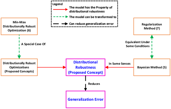
Figure 1: A visualization of the main results in Section 3. A more detailed and informative version is available in Figure 2 of Appendix A.6. In a nutshell, the Bayesian method (5), the DRO method (6), and the regularization method (7) are distributionally robust. Since distributional robustness bounds generalization errors, the three methods can generalize well.

Specifically,

1. Subsection 3.1 formalizes the concept system of “distributional robustness”. In highlights,

   1. Subsection 3.1.1 defines the concepts of distributionally robust optimizations;

   2. Subsection 3.1.2 discusses the practical implementations of the proposed distributionally robust optimization methods;

   3. Subsection 3.1.3 explains that the min-max distributionally robust optimization (6) is a special case of the proposed distributionally robust optimizations;

   4. Subsection 3.1.4 discusses the trade-off between the robustness (to the distributional uncertainty, i.e., unseen data) and the sensitivity/specificity (to the seen training data) for a machine learning model.

2. Subsection 3.2 claims that in the PAC sense, the Bayesian model (5) is distributionally robust.

3. Subsection 3.3 proves that under some conditions, a regularization model (7) is equivalent to a Bayesian model (5).

4. Subsection 3.4 shows that the generalization errors of machine learning models can be bounded by the distributional robustness of these machine learning models, which is a new perspective to the area. Therefore, distributionally robust optimization reduces generalization errors. As a result, the solutions returned by the Bayesian method (5), the (min-max) DRO method (6), and the regularization method (7) are distributionally robust and therefore can generalize well.

5. Subsection 3.5 highlights more differences, other than the inclusion relationship in Subsection 3.1.3, between the proposed “distributionally robust optimization models” in Subsection 3.1 and the existing min-max distributionally robust optimization model (6). In addition, the differences between the existing framework of stability analyses of algorithms (Bousquet and Elisseeff, 2002) and the proposed framework of distributionally robust optimization are also highlighted therein.

3.1 Concept System of Distributional Robustness

Although the concept of “distributional robustness” is philosophically popular, it has not been mathematically defined yet in the literature and is claimed only by the min-max formulation (6). This subsection tries to formalize the concept system of “distributional robustness” and “distributionally robust optimization”, and explain the rationale behind the min-max formulation (6). As a result, distributionally robust optimization models, Bayesian models, and regularization models can be discussed in a common concept system.

Remark 0

For conceptual simplicity and without loss of generality, this subsection assumes that the true problem (1) has only one global optimizer $\bm{x}_{0}\coloneqq\operatorname*{argmin}_{\bm{x}}\mathbb{E}_{\mathbb{P}_{0}}h(\bm{x},\mathbf{\xi})$. $\square$

Considering an optimal value functional (OVF)

$$T:\mathbb{P}\mapsto\min_{\bm{x}\in\mathcal{X}}\mathbb{E}_{\mathbb{P}}h(\bm{x},\mathbf{\xi}),$$ (14)

induced by the true optimization model (1), every specific optimization model $\min_{\bm{x}}\mathbb{E}_{\mathbb{P}}h(\bm{x},\mathbf{\xi})$ is a particularization of the optimal value functional $T$ at $\mathbb{P}$. For example, (1) can be written as $T(\mathbb{P}_{0})$. Also, we define a two-argument cost functional

$$M:(\bm{x},\mathbb{P})\mapsto\mathbb{E}_{\mathbb{P}}h(\bm{x},\mathbf{\xi}).$$ (15)

In this subsection, we consider a set $B_{\epsilon}(\mathbb{P}_{0})$ of nominal distributions centered at the true distribution $\mathbb{P}_{0}$, because what we really care about is the true cost at $\mathbb{P}_{0}$, not the nominal cost at $\bar{\mathbb{P}}$. Hence, $\{\mathbb{P}\mapsto T(\mathbb{P})|\mathbb{P}\in B_{\epsilon}(\mathbb{P}_{0})\}$ defines a set of nominal optimization models centered at the true model $\mathbb{P}_{0}\mapsto T(\mathbb{P}_{0})$.

Definition 0 (Distributional Robustness of Solution)

Suppose $T(\mathbb{P}_{0})$ has only one solution. A point $\bm{x}\in\mathcal{X}$ is an $(\epsilon,L)$-distributionally robust solution to the cost functional $M$, or equivalently the model set $\{\mathbb{P}\mapsto M(\bm{x},P)|\mathbb{P}\in B_{\epsilon}(\mathbb{P}_{0})\}$, at $\mathbb{P}_{0}$ if for every $\mathbb{P}\in B_{\epsilon}(\mathbb{P}_{0})$, we have

$$\Big{|}\mathbb{E}_{\mathbb{P}}h(\bm{x},\mathbf{\xi})-\mathbb{E}_{\mathbb{P}_{0}}h(\bm{x}_{0},\mathbf{\xi})\Big{|}\leq L,$$

where $\bm{x}_{0}\coloneqq\operatorname*{argmin}_{\bm{x}}\mathbb{E}_{\mathbb{P}_{0}}h(\bm{x},\mathbf{\xi})$ and the value of $L$, which is the smallest value satisfying the above display, depends on the values of $\epsilon$ and $\bm{x}$. Here, given $\epsilon$ and $\bm{x}$, $L$ is the robustness measure of the solution $\bm{x}$ for the cost functional $M$ at $\mathbb{P}_{0}$: Given $\epsilon$ and $\bm{x}$, the smaller the value of $L$, the more robust the solution $\bm{x}$ for the cost functional $M$ at $\mathbb{P}_{0}$. $\square$

Note that a robust solution is with respect to a model set rather than a single model. The term “model set” in Definition 3 means $\{\mathbb{P}\mapsto M(\bm{x},\mathbb{P})|\mathbb{P}\in B_{\epsilon}(\mathbb{P}_{0})\}$, rather than $\{\mathbb{P}\mapsto T(\mathbb{P})|\mathbb{P}\in B_{\epsilon}(\mathbb{P}_{0})\}$. This is because, when we discuss the distributional robustness of a robust solution $\bm{x}$ to a model set, all distributions in $B_{\epsilon}(\mathbb{P}_{0})$ share the same solution $\bm{x}$.

Indeed, practically, we expect a robust solution for a model set (centered at the nominal model) because, for example, when the performance (e.g., expected generalization error or expected loss) of a deep learning model is acceptable in multiple testing data sets, we do not want to adjust the parameters of the network (i.e., trained solution) from one to another. For another example, in political policy making, when the external and internal environments do not significantly change, we prefer a policy to be consistent: “Governing a big country is like cooking small fish”; We should not stir the fish too much in cooking so that they will not fall apart into small pieces.

Interested readers are invited to see some additional discussions on the concept of “distributional robustness” in Appendix A.1; One can ignore it without missing the main points of this paper.

An optimization model that finds a distributionally robust solution to an optimization model set is called the distributionally robust counterpart for this model set. Since a model set is usually constructed based on a single model, we can also call the solution-finding optimization model the distributionally robust counterpart for this single model. The example below exemplifies the concept of distributionally robust counterpart.

Example 1

Consider an optimization model $\min_{\bm{x}}\mathbb{E}_{\mathbb{P}_{0}}h(\bm{x},\mathbf{\xi})$ and a set of nominal distributions $B_{\epsilon}(\mathbb{P}_{0})$. If $\bm{x}^{\prime}$ solves the model $\min_{\bm{x}}\mathbb{E}_{\mathbb{P}^{\prime}}h(\bm{x},\mathbf{\xi})$ and $\bm{x}^{\prime}$ is also a distributionally robust solution for the nominal model set induced by $\min_{\bm{x}}\mathbb{E}_{\mathbb{P}_{0}}h(\bm{x},\mathbf{\xi})$ through $B_{\epsilon}(\mathbb{P}_{0})$. Then $\min_{\bm{x}}\mathbb{E}_{\mathbb{P}^{\prime}}h(\bm{x},\mathbf{\xi})$ is a distributionally robust counterpart for $\min_{\bm{x}}\mathbb{E}_{\mathbb{P}_{0}}h(\bm{x},\mathbf{\xi})$. $\square$

3.1.1 Formalization of Distributionally Robust Optimization

For a real-world optimization problem, we aim to find the robust solution for the associated model set and its robustness measure: i.e., the objective value is as still as possible at the given solution when (reasonably small) model perturbations exist. This motivates the definition of the distributionally robust counterpart for the model (1).

Definition 0 (Distributionally Robust Optimization)

The distributionally robust counterpart for the model (1) is defined as

$$\begin{array}[]{cl}\displaystyle\min_{\bm{x},L}&L\\ s.t.&|\mathbb{E}_{\mathbb{P}}h(\bm{x},\mathbf{\xi})-\mathbb{E}_{\mathbb{P}_{0}}h(\bm{x}_{0},\mathbf{\xi})|\leq L\cdot\Delta(\mathbb{P},\mathbb{P}_{0}),~{}~{}~{}\forall\mathbb{P}\in\mathcal{M}(\Xi),\\ &\bm{x}\in\mathcal{X},\end{array}$$ (16)

where $\bm{x}_{0}\coloneqq\operatorname*{argmin}_{\bm{x}}\mathbb{E}_{\mathbb{P}_{0}}h(\bm{x},\mathbf{\xi})$. If (16) has a finite solution $(\bm{x}^{*},L^{*})$, then $\bm{x}^{*}$ is distributionally robust with the relative robustness measure $L^{*}$. $\square$

Interested readers are invited to see more motivations and discussions on Definition 4 in Appendix A.2; One can ignore it without missing the main points of this paper.

The distributionally robust optimization model in Definition 4 is a two-sided version: They limit the cost deviation $\mathbb{E}_{\mathbb{P}}h(\bm{x},\mathbf{\xi})-\mathbb{E}_{\mathbb{P}_{0}}h(\bm{x}_{0},\mathbf{\xi})$ at the solution $\bm{x}$ from both above and below. In practice, people may be only interested in the one-sided versions, that is, the upper bound of the cost difference $\mathbb{E}_{\mathbb{P}}h(\bm{x},\mathbf{\xi})-\mathbb{E}_{\mathbb{P}_{0}}h(\bm{x}_{0},\mathbf{\xi})$ at the solution $\bm{x}$. This reminisces about the two-sided and one-sided generalization errors in machine learning.

Definition 0 (One-Sided Distributionally Robust Optimization)

The one-sided distributionally robust counterpart for the model (1) is defined as

$$\begin{array}[]{cl}\displaystyle\min_{\bm{x},L}&L\\ s.t.&\mathbb{E}_{\mathbb{P}}h(\bm{x},\mathbf{\xi})-\mathbb{E}_{\mathbb{P}_{0}}h(\bm{x}_{0},\mathbf{\xi})\leq L\cdot\Delta(\mathbb{P},\mathbb{P}_{0}),~{}~{}~{}\forall\mathbb{P}\in\mathcal{M}(\Xi),\\ &L\geq 0,\\ &\bm{x}\in\mathcal{X},\end{array}$$ (17)

where $\bm{x}_{0}\coloneqq\operatorname*{argmin}_{\bm{x}}\mathbb{E}_{\mathbb{P}_{0}}h(\bm{x},\mathbf{\xi})$. If (17) has a finite solution $(\bm{x}^{*},L^{*})$, then $\bm{x}^{*}$ is distributionally robust with the one-sided relative robustness measure $L^{*}$. $\square$

3.1.2 Practical Implementations of Distributionally Robust Optimization

In practice, the true distribution $\mathbb{P}_{0}$ might be unknown (e.g., in the data-driven setup) and therefore the optimization problems (16) and (17) cannot be explicitly solved. However, whenever we have a good estimate, say $\bar{\mathbb{P}}$, of $\mathbb{P}_{0}$, we can alternatively resort to the surrogate distributionally robust optimization counterpart of (1).

Definition 0 (Surrogate Distributionally Robust Optimization)

The distributionally robust counterpart for the model (1) at the surrogate $\bar{\mathbb{P}}$ is defined as

$$\begin{array}[]{cl}\displaystyle\min_{\bm{x},L}&L\\ s.t.&|\mathbb{E}_{\mathbb{P}}h(\bm{x},\mathbf{\xi})-\mathbb{E}_{\bar{\mathbb{P}}}h(\bar{\bm{x}},\mathbf{\xi})|\leq L\cdot\Delta(\mathbb{P},\bar{\mathbb{P}}),~{}~{}~{}\forall\mathbb{P}\in\mathcal{M}(\Xi),\\ &\bm{x}\in\mathcal{X},\end{array}$$ (18)

where $\bar{\bm{x}}\coloneqq\operatorname*{argmin}_{\bm{x}}\mathbb{E}_{\bar{\mathbb{P}}}h(\bm{x},\mathbf{\xi})$. For a data-driven problem, $\bar{\mathbb{P}}$ can be chosen as $\hat{\mathbb{P}}_{n}$. $\square$

Problem (18) is therefore termed the distributionally robust counterpart to the nominal Problem (2).

Definition 0 (One-Sided Surrogate Distributionally Robust Optimization)

The one-sided distributionally robust counterpart for the model (1) at the surrogate $\bar{\mathbb{P}}$ is defined as

$$\begin{array}[]{cl}\displaystyle\min_{\bm{x},L}&L\\ s.t.&\mathbb{E}_{\mathbb{P}}h(\bm{x},\mathbf{\xi})-\mathbb{E}_{\bar{\mathbb{P}}}h(\bar{\bm{x}},\mathbf{\xi})\leq L\cdot\Delta(\mathbb{P},\bar{\mathbb{P}}),~{}~{}~{}\forall\mathbb{P}\in\mathcal{M}(\Xi),\\ &L\geq 0,\\ &\bm{x}\in\mathcal{X},\end{array}$$ (19)

where $\bar{\bm{x}}\coloneqq\operatorname*{argmin}_{\bm{x}}\mathbb{E}_{\bar{\mathbb{P}}}h(\bm{x},\mathbf{\xi})$. $\square$

Problem (19) is termed the one-sided distributionally robust counterpart to the nominal Problem (2).

In operations research, an one-sided surrogate distributionally robust optimization model in Definition 7 is termed a Robust Satisficing model (Long et al., 2022). Although the robust satisficing model in Long et al. (2022) is built from other motivations rather than Definition 5 and Definition 7, it works as a specified instance of the proposed distributionally robust optimization framework in Definition 5.

The theorem below provides the rationale for the surrogate distributionally robust optimizations.

Theorem 8 (Surrogate Distributionally Robust Optimization)

Let $(\bm{x}_{1},L_{1})$ solve
the surrogate distributionally robust counterpart (18) at $\bar{\mathbb{P}}$ for the model (1). Then $\bm{x}_{1}$ is distributionally robust with robustness measure $\max\{L_{1},L_{2}\}$, if $\Delta$ is a statistical distance on $\mathcal{M}(\Xi)$ and there exists a non-negative scalar $L_{2}<\infty$ such that

$$|\mathbb{E}_{\bar{\mathbb{P}}}h(\bar{\bm{x}},\mathbf{\xi})-\mathbb{E}_{\mathbb{P}_{0}}h(\bm{x}_{0},\mathbf{\xi})|\leq L_{2}\cdot\Delta(\bar{\mathbb{P}},\mathbb{P}_{0}).$$

(This condition depicts that $\bar{\mathbb{P}}$ is a good estimate of $\mathbb{P}_{0}$: the smaller the value of $L_{2}$, the better.)

Likewise, suppose $(\bm{x}_{1},L_{1})$ solves the one-sided surrogate distributionally robust counterpart (19) at $\bar{\mathbb{P}}$ for the model (1). Then $\bm{x}_{1}$ is distributionally robust with one-sided robustness measure $\max\{L_{1},L_{2}\}$. $\square$

Proof  See Appendix C for the proof based on telescoping and triangle inequalities.  

The condition in Theorem 8 is not restrictive when $\bar{\mathbb{P}}$ is specified by $\hat{\mathbb{P}}_{n}$ in a data-driven setup, due to concentration properties of empirical probability measures; see, e.g., Weed and Bach (2019); Billingsley (1999); Wainwright (2019); Fournier and Guillin (2015).

3.1.3 Min-Max Distributionally Robust Optimization

In what follows, we explain the rationale behind the min-max distributionally robust optimization (6). That is, we aim to find the relation between the min-max distributionally robust optimization (6) and the proposed concept system of “distributional robustness”.

Rationale Behind The Min-Max Robustness.

We start from Definition 4. A special case of Definition 4 can be given if we are only concerned with distributions in a subspace $B_{\epsilon}(\mathbb{P}_{0})\coloneqq\{\mathbb{P}\in\mathcal{M}(\Xi)|\Delta(\mathbb{P},\mathbb{P}_{0})\leq\epsilon\}$ rather than the whole space $\mathcal{M}(\Xi)$, where $\epsilon\geq 0$ is a distributional robustness budget.

Definition 0 (Distributionally Robust Optimization)

The distributionally robust counterpart for the model (1) is defined as

$$\begin{array}[]{cll}\displaystyle\min_{\bm{x},L}&L\\ s.t.&|\mathbb{E}_{\mathbb{P}}h(\bm{x},\mathbf{\xi})-\mathbb{E}_{\mathbb{P}_{0}}h(\bm{x}_{0},\mathbf{\xi})|\leq L,&\forall\mathbb{P}:\Delta(\mathbb{P},\mathbb{P}_{0})\leq\epsilon,\\ &\bm{x}\in\mathcal{X},\end{array}$$ (20)

where $\bm{x}_{0}\coloneqq\operatorname*{argmin}_{\bm{x}}\mathbb{E}_{\mathbb{P}_{0}}h(\bm{x},\mathbf{\xi})$. If (20) has a finite solution $(\bm{x}^{*},L^{*})$, $\bm{x}^{*}$ is a distributionally robust solution with the absolute robustness measure $L^{*}$; cf. Definition 3. $\square$

Compared to Definition 4, Definition 9 is more specific because in practice, sometimes we are only required to consider the smaller distributional space $\{\mathbb{P}\in\mathcal{M}(\Xi)|\Delta(\mathbb{P},\mathbb{P}_{0})\leq\epsilon\}$ rather than the whole space $\mathcal{M}(\Xi)$. This is because additional distributional information $\Delta(\mathbb{P},\mathbb{P}_{0})\leq\epsilon$ is helpful to reduce the conservativeness of a distributionally robust solution. Similarly, a special case of Definition 5 can be given as follows.

Definition 0 (One-Sided Distributionally Robust Optimization)

The one-sided distributionally robust counterpart for the model (1) is defined as

$$\begin{array}[]{cll}\displaystyle\min_{\bm{x},L}&L\\ s.t.&\mathbb{E}_{\mathbb{P}}h(\bm{x},\mathbf{\xi})-\mathbb{E}_{\mathbb{P}_{0}}h(\bm{x}_{0},\mathbf{\xi})\leq L,&\forall\mathbb{P}:\Delta(\mathbb{P},\mathbb{P}_{0})\leq\epsilon,\\ &L\geq 0,\\ &\bm{x}\in\mathcal{X},\end{array}$$ (21)

where $\bm{x}_{0}\coloneqq\operatorname*{argmin}_{\bm{x}}\mathbb{E}_{\mathbb{P}_{0}}h(\bm{x},\mathbf{\xi})$. If (21) has a finite solution $(\bm{x}^{*},L^{*})$, then $\bm{x}^{*}$ is a distributionally robust solution with the one-sided absolute robustness measure $L^{*}$. $\square$

Other than the concepts of “relative robustness measure” and “absolute robustness measure”, we can also define the concept of “local robustness measure”, which is placed in Appendix A.3. Interested readers are invited to see it for additional motivation and deeper understanding. However, one can ignore it without missing the main points of this paper.

In operations research and machine learning practice, the most popular distributionally robust optimization model is the min-max model, which is defined in Definition 11.

Definition 0 (Min-Max Distributionally Robust Optimization)

The min-max distributionally robust counterpart for the model (1) is defined as

$$\begin{array}[]{cl}\displaystyle\min_{\bm{x}}\max_{\mathbb{P}}&\mathbb{E}_{\mathbb{P}}h(\bm{x},\mathbf{\xi})\\ s.t.&\Delta(\mathbb{P},\mathbb{P}_{0})\leq\epsilon,\\ &\bm{x}\in\mathcal{X}.\end{array}$$ (22)

If (22) has a finite solution $(\bm{x}^{*},\mathbb{P}^{*})$, then $\bm{x}^{*}$ is the min-max (i.e., worst-case) distributionally robust solution at the least-favorable (i.e., worst-case) distribution $\mathbb{P}^{*}$. $\square$

We can show that the min-max distributionally robust optimization model is a practical instance of the one-sided distributionally robust optimization model in Definition 10.

Theorem 12 (Min-Max Distributionally Robust Optimization)

Problem (21) is equivalent to Problem (22) in the sense that if $(\bm{x}^{*},L^{*})$ solves (21) and $(\bm{x}^{*},\mathbb{P}^{*})$ solves (22) we have

$$\mathbb{E}_{\mathbb{P}^{*}}h(\bm{x}^{*},\mathbf{\xi})-\mathbb{E}_{\mathbb{P}_{0}}h(\bm{x}_{0},\mathbf{\xi})=L^{*}. \square$$

Proof  See Appendix D. The main idea is to show that Problem (21) can be reformulated to Problem (22), and vice versa.  

Theorem 12 explains why min-max distributionally robust optimization models are valid. However, min-max distributionally robust optimization models are only able to provide one-sided distributional robustness, that is, the upper bound of $\mathbb{E}_{\mathbb{P}}h(\bm{x},\mathbf{\xi})$ at $\bm{x}$. For additional discussions on this point, see Appendix A.4, if interested.

Rationale Behind The Surrogate Min-Max Distributional Robustness.

In what follows, we aim to explore the situation where only the nominal distribution $\bar{\mathbb{P}}$ is available, which is the practical case as in (6).

We begin with Definition 6. A special case of Definition 6 can be given if we are only concerned with distributions in a subspace $B_{\epsilon}(\bar{\mathbb{P}})\coloneqq\{\mathbb{P}\in\mathcal{M}(\Xi)|\Delta(\mathbb{P},\bar{\mathbb{P}})\leq\epsilon\}$ rather than the whole space $\mathcal{M}(\Xi)$.

Definition 0 (Surrogate Distributionally Robust Optimization)

The distributionally robust counterpart for the model (1) at the surrogate $\bar{\mathbb{P}}$ is defined as

$$\begin{array}[]{cl}\displaystyle\min_{\bm{x},L}&L\\ s.t.&|\mathbb{E}_{\mathbb{P}}h(\bm{x},\mathbf{\xi})-\mathbb{E}_{\bar{\mathbb{P}}}h(\bar{\bm{x}},\mathbf{\xi})|\leq L,~{}~{}~{}\forall\mathbb{P}:\Delta(\mathbb{P},\bar{\mathbb{P}})\leq\epsilon,\\ &\bm{x}\in\mathcal{X},\end{array}$$ (23)

where $\bar{\bm{x}}\coloneqq\operatorname*{argmin}_{\bm{x}}\mathbb{E}_{\bar{\mathbb{P}}}h(\bm{x},\mathbf{\xi})$. For a data-driven problem, $\bar{\mathbb{P}}$ can be chosen as $\hat{\mathbb{P}}_{n}$. $\square$

Problem (23) is therefore termed the distributionally robust counterpart to the nominal Problem (2).

The one-sided version is given below.

Definition 0 (One-Sided Surrogate Distributionally Robust Optimization)

The
one-sided distributionally robust counterpart for the model (1) at the surrogate $\bar{\mathbb{P}}$ is defined as

$$\begin{array}[]{cl}\displaystyle\min_{\bm{x},L}&L\\ s.t.&\mathbb{E}_{\mathbb{P}}h(\bm{x},\mathbf{\xi})-\mathbb{E}_{\bar{\mathbb{P}}}h(\bar{\bm{x}},\mathbf{\xi})\leq L,~{}~{}~{}\forall\mathbb{P}:\Delta(\mathbb{P},\bar{\mathbb{P}})\leq\epsilon,\\ &L\geq 0,\\ &\bm{x}\in\mathcal{X},\end{array}$$ (24)

where $\bar{\bm{x}}\coloneqq\operatorname*{argmin}_{\bm{x}}\mathbb{E}_{\bar{\mathbb{P}}}h(\bm{x},\mathbf{\xi})$. For a data-driven problem, $\bar{\mathbb{P}}$ can be chosen as $\hat{\mathbb{P}}_{n}$. $\square$

However, the surrogate distributionally robust optimization in Definition 7 is more general than that in Definition 14 because, for example, in a data-driven setting, $\epsilon$ is not easy to be suitably specified to guarantee that $\mathbb{P}_{0}$ is contained in the empirical $\epsilon$-ball $B_{\epsilon}(\hat{\mathbb{P}}_{n})\coloneqq\{\mathbb{P}\in\mathcal{M}(\Xi)|\Delta(\mathbb{P},\hat{\mathbb{P}}_{n})\leq\epsilon\}$. When $\mathbb{P}_{0}$ is not contained in the empirical $\epsilon$-ball, the data-driven surrogate min-max distributionally robust optimization (24) at $\hat{\mathbb{P}}_{n}$ is meaningless because the true cost at $\mathbb{P}_{0}$ cannot be explicitly upper bounded.

Definition 0 (Surrogate Min-Max Distributionally Robust Optimization)

The surrogate min-max distributionally robust counterpart for the model (1) at the surrogate $\bar{\mathbb{P}}$ is defined as

$$\begin{array}[]{cl}\displaystyle\min_{\bm{x}}\max_{\mathbb{P}}&\mathbb{E}_{\mathbb{P}}h(\bm{x},\mathbf{\xi})\\ s.t.&\Delta(\mathbb{P},\bar{\mathbb{P}})\leq\epsilon,\\ &\bm{x}\in\mathcal{X},\end{array}$$ (25)

which is an instance of (6) when the distributional class $\mathcal{C}$ in (6) is specified by a distributional ball. For a data-driven problem, $\bar{\mathbb{P}}$ can be chosen as $\hat{\mathbb{P}}_{n}$. $\square$

Problem (25) is therefore termed the min-max distributionally robust counterpart of the nominal Problem (2).

Corollary 0 (Surrogate Min-Max Distributionally Robust Optimization)

Problem (24) is equivalent to (25). Therefore, the solutions returned by surrogate min-max distributionally robust optimization models are distributionally robust for the model set centered at the nominal model (2). $\square$

Proof  Compare with Theorem 8 and Theorem 12.  

Corollary 16 explains why surrogate min-max distributionally robust optimization models (6) are most popular in real-world applications.

3.1.4 Robustness and Sensitivity

In the data-driven setup, there is a trade-off between the distributional robustness against distributional model perturbations and the sensitivity/specificity to the (training) data (i.e., the nominal model). To be specific, if a model set (i.e., model functional $T$) has a large robustness measure, the model set has a weak ability to hedge against model perturbations because the objective value is not still in this model set. However, this model set tends to distinguish two similar but different data distributions; i.e., the model set has large resolution in identifying different data distributions. In contrast, if the model set has a small robustness measure, the objective value of this model set is insensitive (i.e., still) to model perturbations, and however, this model set possibly cannot identify two similar but different data distributions either. In practice, we must balance between the robustness against perturbations and the sensitivity/specificity to the collected training data. This motivates us that generalization error bounds might be specified using the distributional robustness: That is, generalization errors can be bounded through the distributional model perturbations; This point will be clearly explained in detail later in Subsection 3.4.

Example 2

The robustness-sensitivity trade-off can be intuitively understood from a life example. The position of a big stone is robust (i.e., still) against a light wind while the position of a piece of cloth is not. However, only this piece of cloth is an indicator of the existence of the light wind; we cannot identify this kind of slight change in air currents through the movement of the big stone. $\square$

The remark below summarizes a new insight for the statistical machine learning community.

Remark 0 (Robustness and Sensitivity)

There is a trade-off between the robustness (to the uncertainty, that is, unseen data) and the sensitivity/specificity (to the training data) for a machine learning model, which reminisces about the bias-variance trade-off. $\square$

3.2 Bayesian Methods

In this subsection, we consider the Bayesian setting (5) to address the modeling uncertainty in $\bar{\mathbb{P}}$ for $\mathbb{P}_{0}$:

$$\min_{\bm{x}\in\mathcal{X}}\mathbb{E}_{\mathbb{Q}}\mathbb{E}_{\mathbb{P}}h(\bm{x},\mathbf{\xi}),$$

where $\mathbb{Q}$ is a probability measure on $(\mathcal{M}(\Xi),\mathcal{B}_{\mathcal{M}(\Xi)})$ and $\mathcal{B}_{\mathcal{M}(\Xi)}$ is the Borel $\sigma$-algebra on $\mathcal{M}(\Xi)$; $\mathbb{P}$ is a random measure which follows $\mathbb{Q}$. In other words, although we do not know the true distribution $\mathbb{P}_{0}$, we know that it is a realization drawn from the distribution $\mathbb{Q}$ rather than simply lies in a distributional ball (i.e., an uncertainty set). This philosophy can be straightforwardly generated in light of the difference between the Frequentists and the Bayesians: Frequentist statistics only assumes that an unknown parameter lies in a space (e.g., a subset of $\mathbb{R}^{n}$) but Bayesian statistics assumes that there exists a (prior) distribution for the unknown parameter. In Bayesian statistics, $\mathbb{P}$ is called a first-order probability measure and $\mathbb{Q}$ is called a second-order probability measure (Gaudard and Hadwin, 1989). In this case, $\mathbb{Q}$ can also be seen as a stochastic process whose realizations are probability measures and $\mathbb{P}$ is a realization of $\mathbb{Q}$ (Ferguson, 1973), (Ghosal and Van der Vaart, 2017, Chap. 3). To clarify further, suppose $(\Xi_{1},\Xi_{2},\cdots,\Xi_{k})$ is an arbitrary $k$-partition of $\Xi$. The probability vector $(\mathbb{P}(\Xi_{1}),\mathbb{P}(\Xi_{2}),\cdots,\mathbb{P}(\Xi_{k}))$ is a random vector whose distribution is specified by $\mathbb{Q}$. Hence, $(\mathbb{Q}(\Xi_{1}),\mathbb{Q}(\Xi_{2}),\cdots,\mathbb{Q}(\Xi_{k}))$ is a stochastic process indexed by the set $\{1,2,\cdots,k\}$ and $(\mathbb{P}(\Xi_{1}),\mathbb{P}(\Xi_{2}),\cdots,\mathbb{P}(\Xi_{k}))$ is a realization. Note that the true distribution $\mathbb{P}_{0}$ can also be seen as a realization of $\mathbb{Q}$ if $\mathbb{P}_{0}$ is in the support set of $\mathbb{Q}$. A good prior $\mathbb{Q}$ should concentrate around $\mathbb{P}_{0}$: it is most ideal that $\mathbb{Q}$ is a Dirac measure at $\mathbb{P}_{0}$ and it is ideal if $\mathbb{P}_{0}$ is the mean distribution of $\mathbb{Q}$.

Theorem 18

If $\bar{\mathbb{P}}$ is the mean of $\mathbb{Q}$ and $\mathbb{E}_{\mathbb{Q}}\mathbb{E}_{\mathbb{P}}|h(\bm{x},\mathbf{\xi})|<\infty$, we have $\mathbb{E}_{\mathbb{Q}}\mathbb{E}_{\mathbb{P}}h(\bm{x},\mathbf{\xi})=\mathbb{E}_{\bar{\mathbb{P}}}h(\bm{x},\mathbf{\xi})$, for every $\bm{x}$. $\square$

Proof  See Appendix E for the proof based on measure-theoretic Funibi’s theorem.  

Theorem 18 generalizes Ferguson (1973, Thm. 3), in which only the Dirichlet process is investigated. Using a Dirichlet process $\mathbb{Q}$ as a prior means that the probability vector $(\mathbb{P}(\Xi_{1}),\mathbb{P}(\Xi_{2}),\cdots,\mathbb{P}(\Xi_{k}))$ follows a Dirichlet distribution. However, Theorem 18 is more a theoretical justification than a useful instruction because, in practice, the most widely used priors on the space of non-parametric probability measures are Dirichlet-process priors and tail-free process priors, attributed to their conjugacy; see Ghosal and Van der Vaart (2017, Chap. 3).

A concrete example of the Bayesian setting (5) is the parametric Bayesian method:

$$\min_{\bm{x}}\mathbb{E}_{\mathbb{Q}_{\bm{\theta}}}\mathbb{E}_{\mathbb{P}_{\mathbf{\xi};\bm{\theta}}}h(\bm{x},\mathbf{\xi}),$$ (26)

where $\mathbb{P}_{\mathbf{\xi};\bm{\theta}}$ is the distribution of $\mathbf{\xi}$, parameterized by $\bm{\theta}\in\mathbb{R}^{q}$, and $\mathbb{Q}_{\bm{\theta}}$ is the distribution of $\bm{\theta}$. In this parametric setting, the true parameter $\bm{\theta}_{0}$ of the true distribution $\mathbb{P}_{\mathbf{\xi};\bm{\theta}_{0}}$ is a realization from $\mathbb{Q}_{\bm{\theta}}$. For a specific parametric example, see Wu et al. (2018). In this paper, we focus on the general non-parametric case as in (5).

The theorem below shows that the solution returned by the Bayesian counterpart (5) for the surrogate model (2) is Probably Approximately Distributionally Robust (PADR).

Theorem 19

Suppose $h$ is a non-negative cost function. The solution $\bar{\bm{x}}$ of the Bayesian counterpart (5) for the surrogate model (2) is probably approximately distributionally robust with absolute robustness measure $L$ with probability at least

$$\max\left\{0,~{}~{}~{}1-\displaystyle\frac{\mathbb{E}_{\mathbb{Q}}\mathbb{E}_{\mathbb{P}}h(\bar{\bm{x}},\mathbf{\xi})+\mathbb{E}_{\mathbb{P}_{0}}h(\bm{x}_{0},\mathbf{\xi})}{L}\right\}. \square$$

Proof  For every $\bm{x}$, since $\mathbb{P}$ is a random measure, $\mathbb{E}_{\mathbb{P}}h(\bm{x},\mathbf{\xi})$ is a random variable and $\mathbb{E}_{\mathbb{Q}}\mathbb{E}_{\mathbb{P}}h(\bm{x},\mathbf{\xi})$ is its mean. According to Markov’s inequality, we have

$$\begin{array}[]{cll}\mathbb{Q}[|\mathbb{E}_{\mathbb{P}}h(\bm{x},\mathbf{\xi})-\mathbb{E}_{\mathbb{P}_{0}}h(\bm{x}_{0},\mathbf{\xi})|\leq L]&\geq 1-\displaystyle\frac{\mathbb{E}_{\mathbb{Q}}|\mathbb{E}_{\mathbb{P}}h(\bm{x},\mathbf{\xi})-\mathbb{E}_{\mathbb{P}_{0}}h(\bm{x}_{0},\mathbf{\xi})|}{L},&\forall\bm{x},\\ &\geq 1-\displaystyle\frac{\mathbb{E}_{\mathbb{Q}}|\mathbb{E}_{\mathbb{P}}h(\bm{x},\mathbf{\xi})|+|\mathbb{E}_{\mathbb{P}_{0}}h(\bm{x}_{0},\mathbf{\xi})|}{L},&\forall\bm{x},\\ &=1-\displaystyle\frac{\mathbb{E}_{\mathbb{Q}}\mathbb{E}_{\mathbb{P}}h(\bm{x},\mathbf{\xi})+\mathbb{E}_{\mathbb{P}_{0}}h(\bm{x}_{0},\mathbf{\xi})}{L},&\forall\bm{x}.\end{array}$$ (27)

Eq. (27) implies that whenever $\mathbb{E}_{\mathbb{Q}}\mathbb{E}_{\mathbb{P}}h(\bm{x},\mathbf{\xi})$ is minimized by $\bar{\bm{x}}$ through (5), the solution $\bar{\bm{x}}$ is distributionally robust with absolute robustness measure $L$ with probability at least

$$\max\left\{0,~{}~{}~{}1-\displaystyle\frac{\mathbb{E}_{\mathbb{Q}}\mathbb{E}_{\mathbb{P}}h(\bar{\bm{x}},\mathbf{\xi})+\mathbb{E}_{\mathbb{P}_{0}}h(\bm{x}_{0},\mathbf{\xi})}{L}\right\}.$$

This completes the proof. (Note that $L$ needs to be specified to a sufficiently large value. Otherwise, the probability on the right side of (27) cannot be sufficiently large.)  

3.2.1 Data-Driven Case

In the data-driven setting, the most popular non-parametric Bayesian prior for $\mathbb{Q}$ is the Dirichlet-process prior, whose posterior mean distribution, after observing $n$ i.i.d. samples, is given by (Ferguson, 1973), (Ghosal and Van der Vaart, 2017, Chap. 3)

$$\frac{\alpha}{\alpha+n}\hat{\mathbb{P}}+\frac{n}{\alpha+n}\hat{\mathbb{P}}_{n},$$

where $\hat{\mathbb{P}}$ is a prior estimate of $\mathbb{P}_{0}$ based on our prior belief and $\alpha$ is a non-negative scalar used to adjust our trust level of $\hat{\mathbb{P}}$: the larger the value of $\alpha$, the more trust we have towards $\hat{\mathbb{P}}$. This can be seen as a mixture distribution of $\hat{\mathbb{P}}$ and $\hat{\mathbb{P}}_{n}$ with mixing weights $\frac{\alpha}{\alpha+n}$ and $\frac{n}{\alpha+n}$, respectively: i.e., a weighted combination of prior knowledge and data evidence. As $n\to\infty$, the weight of the prior belief $\hat{\mathbb{P}}$ decays quickly, which is consistent with our intuition that as the sample size gets larger, we should trust more on the empirical distribution $\hat{\mathbb{P}}_{n}$ due to the concentration property of $\hat{\mathbb{P}}_{n}$, i.e., the weak convergence of $\hat{\mathbb{P}}_{n}$ to $\mathbb{P}_{0}$ (e.g., recall the Portmanteau theorem). One may also be reminiscent of (11), i.e., a concentration property defined by Wasserstein distance; Note that the Wasserstein distance metrizes this weak convergence (Weed and Bach, 2019).

As a result of Theorem 18, if we use the Dirichlet-process prior, the Bayesian model (5) is particularized into

$$\min_{\bm{x}}\frac{\alpha}{\alpha+n}\mathbb{E}_{\hat{\mathbb{P}}}h(\bm{x},\mathbf{\xi})+\frac{n}{\alpha+n}\mathbb{E}_{\hat{\mathbb{P}}_{n}}h(\bm{x},\mathbf{\xi}).$$ (28)

We can further generalize (28) into

$$\min_{\bm{x}}\beta_{n}\mathbb{E}_{\hat{\mathbb{P}}}h(\bm{x},\mathbf{\xi})+(1-\beta_{n})\mathbb{E}_{\hat{\mathbb{P}}_{n}}h(\bm{x},\mathbf{\xi}),$$ (29)

where $\beta_{n}\in[0,1]$ is not necessarily equal to $\frac{\alpha}{\alpha+n}$ but we still require that $\beta_{n}\to 0$, as $n\to\infty$.

3.3 Regularized Sample-Average Approximation

We re-arrange (29) to see

$$(1-\beta_{n})\min_{\bm{x}}\mathbb{E}_{\hat{\mathbb{P}}_{n}}h(\bm{x},\mathbf{\xi})+\lambda_{n}\cdot f(\bm{x}),$$ (30)

which is equivalent to solve

$$\min_{\bm{x}}\mathbb{E}_{\hat{\mathbb{P}}_{n}}h(\bm{x},\mathbf{\xi})+\lambda_{n}\cdot f(\bm{x}),$$ (31)

where $\lambda_{n}\coloneqq\frac{\beta_{n}}{1-\beta_{n}}$ and $f(\bm{x})\coloneqq\mathbb{E}_{\hat{\mathbb{P}}}h(\bm{x},\mathbf{\xi})$. Obviously, (31) is a regularized SAA (i.e., regularized ERM) optimization model, which is popular in applied statistics and, especially, machine learning, where $f(\bm{x})$ is a regularizer (e.g., any norm of $\bm{x}$). One may recall the Ridge regression where $f(\bm{x})\coloneqq\|\bm{x}\|_{2}$ and LASSO (least absolute shrinkage and selection operator) regression where $f(\bm{x})\coloneqq\|\bm{x}\|_{1}$.

Theorem 20

Let $\mathbb{Q}$ be a Dirichlet-process prior. For every specified regularizer $f(\bm{x})$, if there exists a probability measure $\hat{\mathbb{P}}$ such that

$$f(\bm{x})=\mathbb{E}_{\hat{\mathbb{P}}}h(\bm{x},\mathbf{\xi}),~{}~{}~{}\forall\bm{x},$$ (32)

then the regularized SAA model (31) is equivalent to the Bayesian model (5). Therefore, any Bayesian model (5) is adding a regularizer $f(\bm{x})$ (induced by $\hat{\mathbb{P}}$) to the empirical model $\min_{\bm{x}}\mathbb{E}_{\hat{\mathbb{P}}_{n}}h(\bm{x},\mathbf{\xi})$. Also, any regularized SAA optimization method is a Bayesian method whose solution $\bar{\bm{x}}$ is probably approximately distributionally robust with absolute robustness measure $L$ with probability at least

$$\max\left\{0,~{}~{}~{}1-\displaystyle\frac{\mathbb{E}_{\mathbb{Q}}|\mathbb{E}_{\mathbb{P}}h(\bar{\bm{x}},\mathbf{\xi})-\mathbb{E}_{\mathbb{P}_{0}}h(\bm{x}_{0},\mathbf{\xi})|}{L}\right\},$$

where $\mathbb{Q}$ is a Dirichlet-process-like prior with posterior mean $\beta_{n}\hat{\mathbb{P}}+(1-\beta_{n})\hat{\mathbb{P}}_{n}$. Further, if $h$ is non-negative, which is usually the case in supervised machine learning (Wang et al., 2022), $\bar{\bm{x}}$ is probably approximately distributionally robust with absolute robustness measure $L$ with probability at least

$$\begin{array}[]{l}1-\displaystyle\frac{\mathbb{E}_{\mathbb{P}_{0}}h(\bm{x}_{0},\mathbf{\xi})}{L}-\displaystyle\frac{\mathbb{E}_{\mathbb{Q}}\mathbb{E}_{\mathbb{P}}h(\bar{\bm{x}},\mathbf{\xi})}{L},\\ \quad\quad=1-\displaystyle\frac{\mathbb{E}_{\mathbb{P}_{0}}h(\bm{x}_{0},\mathbf{\xi})}{L}-\beta_{n}\displaystyle\frac{\mathbb{E}_{\hat{\mathbb{P}}}h(\bar{\bm{x}},\mathbf{\xi})}{L}-(1-\beta_{n})\displaystyle\frac{\mathbb{E}_{\hat{\mathbb{P}}_{n}}h(\bar{\bm{x}},\mathbf{\xi})}{L},\end{array}$$

if it is non-negative.

Proof  See Appendix F. Given a regularizer $f(\bm{x})$, we can construct a Bayesian non-parametric prior $\hat{\mathbb{P}}$, and vice versa.  

Remark 0

In Theorem 20, we require $\mathbb{Q}$ to be a Dirichlet-process prior so that the equivalence between the regularization model (7) and the Bayesian model (5) holds. In general, the equivalence is no longer true but an inclusion relationship holds. To be specific, a regularization model (7) can be transformed into a Bayesian model (5) by constructing $\hat{\mathbb{P}}$ satisfying (32). But a Bayesian model (5) cannot be transformed into a regularization model (7) if $\mathbb{Q}$ is not a Dirichlet process prior. $\square$

The condition in (32) is not restrictive, and $\hat{\mathbb{P}}$ can be constructed using $f(\bm{x})$ and $h(\bm{x},\mathbf{\xi})$. For example, when $\Xi$ is bounded, $\hat{\mathbb{P}}$ can be chosen as the uniform distribution on $\Xi$ with density function

$$\frac{\mathrm{d}\hat{\mathbb{P}}}{\mathrm{d}\mathcal{L}}\coloneqq\frac{f(\bm{x})}{\int_{\Xi}h(\bm{x},\mathbf{\xi})\mathrm{d}\xi},~{}~{}~{}\forall\bm{x},$$

where $\mathcal{L}$ is the Lebesgue measure on $(\Xi,\mathcal{B}_{\Xi})$ and the left side of the above display is the Radon–Nikodym derivative of $\hat{\mathbb{P}}$ with respect to $\mathcal{L}$. For another example when $\Xi$ is unbounded, see Appendix A.5.

3.3.1 Probabilistic Interpretations of Regularized SAA Models

Different from the deterministic learning problem (1), the randomized learning counterpart [i.e., Gibbs algorithm (Germain et al., 2009)]

$$\min_{\mathbb{Q}_{\bm{x}}}\mathbb{E}_{\mathbb{Q}_{\bm{x}}}\mathbb{E}_{\mathbb{P}_{0}}h(\bm{x},\mathbf{\xi}),$$ (33)

where $\mathbb{Q}_{\bm{x}}$ is a distribution on $\mathcal{X}$, is also standard in its own right.

Usually, the regularized problem (31) is interpreted from the randomized learning perspective (33) and a prior distribution $\Pi_{\bm{x}}$ on $\mathcal{X}$, which encodes our prior belief on the hypothesis class $\mathcal{X}$, is used. For example, one may be reminiscent of the PAC-Bayesian theory, that is, the information empirical risk minimization model (Germain et al., 2016, Sec. 2)

$$\min_{\mathbb{Q}_{\bm{x}}}\mathbb{E}_{\mathbb{Q}_{\bm{x}}}\mathbb{E}_{\hat{\mathbb{P}}_{n}}h(\bm{x},\mathbf{\xi})+\lambda\operatorname{KL}(\mathbb{Q}_{\bm{x}}||\Pi_{\bm{x}}),$$ (34)

where $\operatorname{KL}(\mathbb{Q}_{\bm{x}}||\Pi_{\bm{x}})$ denotes the Kullback–Leibler divergence of $\mathbb{Q}_{\bm{x}}$ from $\Pi_{\bm{x}}$. Note that when $\mathbb{Q}_{\bm{x}}$ is a point-mass distribution, the information empirical risk minimization model reduces to (31) and $f(\bm{x})\coloneqq-\log\pi(\bm{x})$, in which $\pi(\bm{x})$ is the density function of $\Pi_{\bm{x}}$ with respect to the Lebesgue measure. In this case, if $\Pi_{\bm{x}}$ is a Gaussian (resp. Laplacian) distribution, we have the Ridge (resp. LASSO) regression model.

In contrast to the PAC-Bayesian viewpoint (34), this paper provides a new Bayesian probabilistic interpretation for regularized SAA methods if the condition (32) holds; see Theorem 20. The difference between the two Bayesian perspectives lies in over which space we assign a prior distribution: The prior distribution $\mathbb{Q}_{\bm{x}}$ on the hypothesis class $\mathcal{X}$ or the prior distribution $\mathbb{Q}$ of the data distribution $\mathbb{P}$ in the distribution class $\mathcal{C}$; cf. (34) and (5). Therefore, when we face distributional uncertainty in the nominal distribution $\bar{\mathbb{P}}$ for the true distribution $\mathbb{P}_{0}$, we have two possible Bayesian philosophies to hedge against it: The first one is to introduce a prior belief on the hypothesis to reduce the uncertainty (i.e., which hypotheses are relatively more important than others); The second one is to assign a prior belief on the nominal data distributions (i.e., which nominal data distributions are relatively more important than others). The interesting result is that both the two ideas lead to the same technical methodology—the regularized empirical risk minimization model (31).

The remark below summarizes a new insight for the statistical machine learning community.

Remark 0

Hedging against the distributional uncertainty in the data distribution is equivalent to considering a prior belief on the hypothesis class, and vice versa. $\square$

This philosophy can also be supported by Bertsimas and Copenhaver (2018) through examining the (conditional) equivalence between regularization and robustness in linear and matrix regression; see, e.g., Corollary 1 therein. The difference is that the equivalence between regularization and robustness in Bertsimas and Copenhaver (2018) is not in the distributional/probabilistic but in the deterministic sense: There is no probability distribution involved and only norm-based uncertainty sets for real-valued parameters are discussed.

3.3.2 On Bias-Variance Trade-Off

Although regularized SAA methods are originally invented from the motivation of bias-variance trade-off (i.e., penalizing the complexity of the hypothesis class), we have shown that solving them is equivalent to solving Bayesian models, and therefore, regularized SAA methods are probably approximately distributionally robust optimization models. The bias-variance trade-off shows that by introducing a bias term $\lambda_{n}f(\bm{x})$ for an estimator, it is possible to reduce the variance of the estimator. This can be explicitly understood from (29): By introducing the bias term $\beta_{n}\mathbb{E}_{\hat{\mathbb{P}}}h(\bm{x},\mathbf{\xi})$, the variance of $(1-\beta_{n})\mathbb{E}_{\hat{\mathbb{P}}_{n}}h(\bm{x},\mathbf{\xi})$ reduces $(1-\beta_{n})^{2}$ times compared with $\mathbb{E}_{\hat{\mathbb{P}}_{n}}h(\bm{x},\mathbf{\xi})$. To clarify further, for every $\bm{x}$, the mean of the objective of (29) is

$$\begin{array}[]{cl}\mathbb{E}_{\mathbb{P}^{n}_{0}}[\beta_{n}\mathbb{E}_{\hat{\mathbb{P}}}h(\bm{x},\mathbf{\xi})+(1-\beta_{n})\mathbb{E}_{\hat{\mathbb{P}}_{n}}h(\bm{x},\mathbf{\xi})]\par&=\beta_{n}\mathbb{E}_{\hat{\mathbb{P}}}h(\bm{x},\mathbf{\xi})+(1-\beta_{n})\mathbb{E}_{\mathbb{P}^{n}_{0}}\mathbb{E}_{\hat{\mathbb{P}}_{n}}h(\bm{x},\mathbf{\xi})\\ &=\beta_{n}\mathbb{E}_{\hat{\mathbb{P}}}h(\bm{x},\mathbf{\xi})+(1-\beta_{n})\mathbb{E}_{\mathbb{P}_{0}}h(\bm{x},\mathbf{\xi}),\end{array}$$

which is biased from the true mean $\mathbb{E}_{\mathbb{P}_{0}}h(\bm{x},\mathbf{\xi})$. But the objective function of (29) has the variance that is $(1-\beta_{n})^{2}$ times lower than that of $\mathbb{E}_{\hat{\mathbb{P}}_{n}}h(\bm{x},\mathbf{\xi})$. Note that if $\hat{\mathbb{P}}$ could be elegantly given, the performance gap of the model (29) would be smaller than that of the SAA model $\min_{\bm{x}}\mathbb{E}_{\hat{\mathbb{P}}_{n}}h(\bm{x},\mathbf{\xi})$ because for every $\bm{x}$

$$\begin{array}[]{l}|\beta_{n}\mathbb{E}_{\hat{\mathbb{P}}}h(\bm{x},\mathbf{\xi})+(1-\beta_{n})\mathbb{E}_{\hat{\mathbb{P}}_{n}}h(\bm{x},\mathbf{\xi})-\mathbb{E}_{\mathbb{P}_{0}}h(\bm{x},\mathbf{\xi})|\\ \quad\quad\leq\beta_{n}|\mathbb{E}_{\hat{\mathbb{P}}}h(\bm{x},\mathbf{\xi})-\mathbb{E}_{\mathbb{P}_{0}}h(\bm{x},\mathbf{\xi})|+(1-\beta_{n})|\mathbb{E}_{\hat{\mathbb{P}}_{n}}h(\bm{x},\mathbf{\xi})-\mathbb{E}_{\mathbb{P}_{0}}h(\bm{x},\mathbf{\xi})|\\ \quad\quad\leq|\mathbb{E}_{\hat{\mathbb{P}}_{n}}h(\bm{x},\mathbf{\xi})-\mathbb{E}_{\mathbb{P}_{0}}h(\bm{x},\mathbf{\xi})|,\end{array}$$

if $|\mathbb{E}_{\hat{\mathbb{P}}}h(\bm{x},\mathbf{\xi})-\mathbb{E}_{\mathbb{P}_{0}}h(\bm{x},\mathbf{\xi})|\leq|\mathbb{E}_{\hat{\mathbb{P}}_{n}}h(\bm{x},\mathbf{\xi})-\mathbb{E}_{\mathbb{P}_{0}}h(\bm{x},\mathbf{\xi})|$ (i.e., $\hat{\mathbb{P}}$ is a good estimate of $\mathbb{P}_{0}$; $\hat{\mathbb{P}}$ is better than $\hat{\mathbb{P}}_{n}$).

Hence, if $f(\bm{x})$ is a good regularizer and $\lambda_{n}$ is a good regularization coefficient, the regularized SAA model (31) is potential to give lower generalization error than the standard SAA method because the former has a smaller robustness measure than that of the latter. Note that in the Bayesian setting (5), the probably approximately distributional robustness measure $L$ in Theorem 19 and (27) can be seen as a type of upper bounds of generalization errors. (For details, see Subsection 3.4.)

In summary, through the lens of the concept of distributional robustness and the non-parametric Bayesian model (29) using a Dirichlet-process-like prior whose posterior mean is $\beta_{n}\hat{\mathbb{P}}+(1-\beta_{n})\hat{\mathbb{P}}_{n}$, we can see that there is a close relation among Bayesian methods, DRO methods, and regularized SAA methods. Details can be revisited from Theorems 19 and 20. In addition, the bias-variance trade-off is in analogy to the robustness-sensitivity trade-off discussed in Subsection 3.1.4: They are explaining the same phenomenon (i.e., the negative impact of the uncertainty in the nominal distribution versus the positive impact of the useful information in the nominal distribution) from two different perspectives.

Remark 0

Subsections 3.1, 3.2, and 3.3 have defined several new concepts and established the relations between them and the existing ones. Confused readers are invited to see Appendix A.6 for a detailed visual clarification before proceeding to the next subsection; One may ignore it without missing the main points in this paper if he/she is clear about the relationships among concepts. $\square$

3.4 Distributional Robustness and Generalization Error

In this subsection, we consider the data-driven case where the empirical distribution $\hat{\mathbb{P}}_{n}$ is involved. Let $\bar{\mathbb{P}}$ be a surrogate of $\mathbb{P}_{0}$ constructed from data. For example, $\bar{\mathbb{P}}$ can be $\hat{\mathbb{P}}_{n}$ in an SAA model. For another example, $\bar{\mathbb{P}}$ can be $\beta_{n}\hat{\mathbb{P}}+(1-\beta_{n})\hat{\mathbb{P}}_{n}$ in a regularized SAA (i.e., a Bayesian) model where $\hat{\mathbb{P}}$ is a prior belief of $\mathbb{P}_{0}$. Recall from Subsection 2.2 that in the machine learning literature, the probably approximately correct (PAC) generalization error bound $L_{\bm{x},\eta}$ with probability at least $1-\eta$ of a solution $\bm{x}$ is defined as

$$\mathbb{P}_{0}^{n}[\mathbb{E}_{\mathbb{P}_{0}}h(\bm{x},\mathbf{\xi})-\mathbb{E}_{\bar{\mathbb{P}}}h(\bm{x},\mathbf{\xi})\leq L_{\bm{x},\eta}]\geq 1-\eta$$

for the one-sided case and as

$$\mathbb{P}_{0}^{n}[|\mathbb{E}_{\mathbb{P}_{0}}h(\bm{x},\mathbf{\xi})-\mathbb{E}_{\bar{\mathbb{P}}}h(\bm{x},\mathbf{\xi})|\leq L_{\bm{x},\eta}]\geq 1-\eta$$

for the two-sided case. In addition, the expected generalization error bound $L_{\bm{x}}$ of a solution $\bm{x}$ is defined as

$$\mathbb{E}_{\mathbb{P}_{0}^{n}}[\mathbb{E}_{\mathbb{P}_{0}}h(\bm{x},\mathbf{\xi})-\mathbb{E}_{\bar{\mathbb{P}}}h(\bm{x},\mathbf{\xi})]\leq L_{\bm{x}}$$

or

$$\mathbb{E}_{\mathbb{P}_{0}^{n}}[|\mathbb{E}_{\mathbb{P}_{0}}h(\bm{x},\mathbf{\xi})-\mathbb{E}_{\bar{\mathbb{P}}}h(\bm{x},\mathbf{\xi})|]\leq L_{\bm{x}}.$$

In this subsection, we are concerned with the uniform generalization error $|\mathbb{E}_{\mathbb{P}_{0}}h(\bm{x},\mathbf{\xi})-\mathbb{E}_{\bar{\mathbb{P}}}h(\bm{x},\mathbf{\xi})|$, for every $\bm{x}$, and the ad-hoc generalization error $|\mathbb{E}_{\mathbb{P}_{0}}h(\bar{\bm{x}},\mathbf{\xi})-\mathbb{E}_{\bar{\mathbb{P}}}h(\bar{\bm{x}},\mathbf{\xi})|$ of the nominal model $\min_{\bm{x}}\mathbb{E}_{\bar{\mathbb{P}}}h(\bm{x},\mathbf{\xi})$ at the solution $\bar{\bm{x}}$, where $\bar{\bm{x}}\in\operatorname*{argmin}_{\bm{x}}\mathbb{E}_{\bar{\mathbb{P}}}h(\bm{x},\mathbf{\xi})$.

Usually, the generalization error bounds of machine learning models are specified by

1. Measure concentration inequalities such as Hoeffding’s and Bernstein inequalities (Wainwright, 2019, Chaps. 2-3), McDiarmid’s inequality (Zhang and Chen, 2021), Variation-Based Concentration (Gao, 2022, Thm. 1 and Cors. 1-2), among many others (Zhang and Chen, 2021). In this case, the properties of the cost function $h(\bm{x},\mathbf{\xi})$ such as the boundedness and Lipschitz-norm are leveraged;

2. Richness of hypothesis classes such as VC dimension and Rademacher complexity (Wainwright, 2019, Chap. 4);

3. PAC-Bayesian arguments through the KL-Divergence of the posterior hypothesis distribution from the prior hypothesis distribution (Germain et al., 2016, Sec. 2), etc.;

4. Information-theoretic methods through mutual information (Xu and Raginsky, 2017) or Wasserstein distance (Wang et al., 2019; Rodríguez Gálvez et al., 2021) between the posterior hypothesis distribution and the (training) data distribution, etc.

The PAC-Bayesian arguments describe the generalization error bounds of a machine learning model by the (statistical) difference between the prior distribution $\Pi_{\bm{x}}$ of the hypothesis class $\mathcal{X}$, as used in (34), and the optimal randomized decision $\mathbb{Q}_{\bm{x}}$ that solves the randomized-learning model $\min_{\mathbb{Q}_{\bm{x}}}\mathbb{E}_{\mathbb{Q}_{\bm{x}}}\mathbb{E}_{\mathbb{P}_{0}}h(\bm{x},\mathbf{\xi})$. In contrast, information-theoretic methods depict the generalization error bounds of a machine learning model by the (statistical) difference between the posterior distribution $\mathbb{Q}_{\bm{x}}$ of hypothesis and the training data distribution $\hat{\mathbb{P}}_{n}$; i.e., how much does the posterior distribution $\mathbb{Q}_{\bm{x}}$ of hypothesis depend on the training data $\hat{\mathbb{P}}_{n}$? In this subsection, we establish the generalization error bounds of a machine learning model using its distributional robustness measures, that is, using the (statistical) difference between the training data distribution $\hat{\mathbb{P}}_{n}$ (or the transformed training data distribution $\bar{\mathbb{P}}$) and the population data distribution $\mathbb{P}_{0}$. This is a new perspective to characterize and bound generalization errors. The main point here is that the generalization errors of a machine learning model can be specified through several yet extremely different ways.

3.4.1 Uniform Generalization Error Through Distributional Uncertainty

The uniform generalization error bound is straightforward to establish due to the weak convergence of $\bar{\mathbb{P}}$ to $\mathbb{P}_{0}$, that is, $\Delta(\mathbb{P}_{0},\bar{\mathbb{P}})\to 0$, $\mathbb{P}^{n}_{0}$-almost surely (Weed and Bach, 2019), and the continuity of the linear functional $\mathbb{P}\mapsto\mathbb{E}_{\mathbb{P}}h(\bm{x},\mathbf{\xi})<\infty$, where $\Delta$ denotes the Wasserstein distance. (Note that the Wasserstein distance metrizes the weak topology on $\mathcal{M}(\Xi)$.) The result in the proposition below is standard and well-established in the mathematical statistics literature. We borrow it to describe and characterize generalization errors from a new perspective, the perspective of distributional uncertainty.

Proposition 0 (Uniform Generalization Error Through Distributional Uncertainty)

For every $\bm{x}$, if the cost function $h(\bm{x},\cdot)$ is $L(\bm{x})$-Lipschitz continuous in $\mathbf{\xi}$ on $\Xi$, we have

$$|\mathbb{E}_{\mathbb{P}_{0}}h(\bm{x},\mathbf{\xi})-\mathbb{E}_{\bar{\mathbb{P}}}h(\bm{x},\mathbf{\xi})|\leq L(\bm{x})\Delta(\mathbb{P}_{0},\bar{\mathbb{P}}),~{}~{}~{}\forall\bm{x},$$

$\mathbb{P}^{n}_{0}$-almost surely, where $\Delta$ is the order-$1$ Wasserstein distance. $\square$

Proof  See Appendix G for the proof based on the definition of Wasserstein distance.  

Proposition 24 implies that the smaller the distributional uncertainty in $\bar{\mathbb{P}}$ is, the smaller the generalization error is. In addition, the generalization error is also affected by the Lipschitz constant of the cost function, and therefore, a cost function that has a smaller Lipschitz constant is preferable; This explains why, for example, Huber’s loss function is better than the square loss function because the former has a smaller Lipschitz constant. Note that the variable $L$ (i.e., robustness measure) in Definition 4 and Definition 6 depends on $\bm{x}$ because they are simultaneously involved in a common optimization problem (16) and (18), respectively. However, the Lipschitz constant $L(\bm{x})$ in Proposition 24 depends on $\bm{x}$ just due to the innate property of the cost function $h(\bm{x},\mathbf{\xi})$.

Remark 0

The order-$1$ Wasserstein distance in Proposition 24 can be replaced with any order-$p$ Wasserstein distance where $p\geq 2$ because for any two distributions $\mathbb{P}_{1}$ and $\mathbb{P}_{2}$, we have $W_{p}(\mathbb{P}_{1},\mathbb{P}_{2})\leq W_{q}(\mathbb{P}_{1},\mathbb{P}_{2})$ where $1\leq p\leq q\leq\infty$. This fact is attributed to Givens and Shortt (1984, Prop. 3); see also Römisch and Schultz (1991, Rem. 2.2). $\square$

Corollary 0

For every $\bm{x}$, if the cost function $h(\bm{x},\cdot)$ is $L(\bm{x})$-Lipschitz continuous in $\mathbf{\xi}$ on $\Xi$, we have the expected uniform generalization error bound $\mathbb{E}_{\mathbb{P}^{n}_{0}}|\mathbb{E}_{\mathbb{P}_{0}}h(\bm{x},\mathbf{\xi})-\mathbb{E}_{\bar{\mathbb{P}}}h(\bm{x},\mathbf{\xi})|\leq L(\bm{x})\mathbb{E}_{\mathbb{P}^{n}_{0}}\Delta(\mathbb{P}_{0},\bar{\mathbb{P}})$, for every $\bm{x}$. $\square$

The one-sided versions of Proposition 24 and Corollary 26 are straightforward to claim by requiring (the one-sided Lipschitz continuity)

$$h(\bm{x},\mathbf{\xi})-h(\bm{x},\bar{\mathbf{\xi}})\leq L(\bm{x})\|\mathbf{\xi}-\bar{\mathbf{\xi}}\|$$

for every $\mathbf{\xi},\bar{\mathbf{\xi}}\in\Xi$. We do not give details in this paper.

A concrete example of Proposition 24 is given as

$$|\mathbb{E}_{\mathbb{P}_{0}}h(\bm{x},\mathbf{\xi})-\mathbb{E}_{\hat{\mathbb{P}}_{n}}h(\bm{x},\mathbf{\xi})|\leq L(\bm{x})\Delta(\mathbb{P}_{0},\hat{\mathbb{P}}_{n}),~{}~{}~{}\forall\bm{x},$$

$\mathbb{P}^{n}_{0}$-almost surely. The $L(\bm{x})$-Lipschitz continuity is not restrictive for a machine learning model because the cost function $h$ can be elegantly designed; cf. Wang et al. (2022).

3.4.2 Generalization Error Through Distributional Robustness

In what follows, we focus on the generalization error of the nominal model $\min_{\bm{x}}\mathbb{E}_{\bar{\mathbb{P}}}h(\bm{x},\mathbf{\xi})$ at its optimal solution $\bar{\bm{x}}$. Note that, in practical implementation of a machine learning model, we are more interested in the generalization capability of a specified hypothesis, for example, a regression model with already-optimized coefficients.

Theorem 27 (Generalization Error Through Absolute Robustness Measure)

Suppose $\mathbb{P}_{0}$ is contained in $B_{\epsilon}(\bar{\mathbb{P}})\coloneqq\{\mathbb{P}\in\mathcal{M}(\Xi)|\Delta(\mathbb{P},\bar{\mathbb{P}})\leq\epsilon\}$ and $(\bm{x}^{*},L^{*})$ solves the surrogate distributionally robust optimization model (23), i.e.,

$$\begin{array}[]{cll}\displaystyle\min_{\bm{x},L}&L\\ s.t.&|\mathbb{E}_{\mathbb{P}}h(\bm{x},\mathbf{\xi})-\mathbb{E}_{\bar{\mathbb{P}}}h(\bar{\bm{x}},\mathbf{\xi})|\leq L,&\forall\mathbb{P}:\Delta(\mathbb{P},\bar{\mathbb{P}})\leq\epsilon,\\ &\bm{x}\in\mathcal{X}.\end{array}$$

If $h(\bm{x},\mathbf{\xi})$ is $L(\mathbf{\xi})$-Lipschitz continuous in $\bm{x}$ on $\mathcal{X}$, for every $\mathbf{\xi}\in\Xi$, then the generalization error $|\mathbb{E}_{\mathbb{P}_{0}}h(\bar{\bm{x}},\mathbf{\xi})-\mathbb{E}_{\bar{\mathbb{P}}}h(\bar{\bm{x}},\mathbf{\xi})|$ of the nominal model $\min_{\bm{x}}\mathbb{E}_{\bar{\mathbb{P}}}h(\bm{x},\mathbf{\xi})$ is upper bounded by

$$\|\bar{\bm{x}}-\bm{x}^{*}\|\cdot\mathbb{E}_{\mathbb{P}_{0}}L(\mathbf{\xi})+L^{*},$$

$\mathbb{P}^{n}_{0}$-almost surely. In addition, the generalization error $|\mathbb{E}_{\mathbb{P}_{0}}h(\bm{x}^{*},\mathbf{\xi})-\mathbb{E}_{\mathbb{P}^{*}}h(\bm{x}^{*},\mathbf{\xi})|$ of the surrogate distributionally robust optimization model (23) is upper bounded by

$$2L^{*},$$

$\mathbb{P}^{n}_{0}$-almost surely. $\square$

Proof  See Appendix H for the proof based on telescoping and triangle inequalities.  

Note that Theorem 27 holds almost surely, not in the PAC sense, and therefore, generalization error bounds specified by absolute robustness measures are stronger than those specified in the PAC sense.

Remark 0

If $\mathbb{P}_{0}$ is contained in $B_{\epsilon}(\bar{\mathbb{P}})\coloneqq\{\mathbb{P}\in\mathcal{M}(\Xi)|\Delta(\mathbb{P},\bar{\mathbb{P}})\leq\epsilon\}$ in $\mathbb{P}^{n}_{0}$-probability, for example, as in (11), then Theorem 27 holds in $\mathbb{P}^{n}_{0}$-probability. $\square$

Corollary 0 (Generalization Error Through Absolute Robustness Measure)

Under the settings of Theorem 27, the expected generalization errors are given by

$$\mathbb{E}_{\mathbb{P}_{0}^{n+1}}L(\mathbf{\xi})\|\bar{\bm{x}}-\bm{x}^{*}\|+\mathbb{E}_{\mathbb{P}^{n}_{0}}L^{*},$$

and $2\mathbb{E}_{\mathbb{P}^{n}_{0}}[L^{*}]$, respectively. Note that $\bar{\bm{x}}$, $\bm{x}^{*}$, and $L^{*}$ depend on the specific choice of the training data. $\square$

Proof  See Appendix I.  

The term $|\mathbb{E}_{\mathbb{P}_{0}}h(\bar{\bm{x}},\mathbf{\xi})-\mathbb{E}_{\mathbb{P}_{0}}h(\bm{x}^{*},\mathbf{\xi})|$ can be upper bounded by other possible ways rather than the Lipschitz continuity of $h$. We use Lipschitz continuity just as an example. For a machine learning model, if $h$ is continuous in $\bm{x}$ and bounded on a compact feasible region $\mathcal{X}$, the Lipschitz continuity is naturally guaranteed. Fortunately, the continuity and boundedness condition is not practically restrictive; see, e.g., Wang et al. (2022).

Theorem 27 and Corollary 29 reveal that whenever the DRO model (23) is solved, the (expected) generalization errors of the nominal model $\min_{\bm{x}}\mathbb{E}_{\bar{\mathbb{P}}}h(\bm{x},\mathbf{\xi})$ and the surrogate distributionally robust optimization model (23) are also controlled by the absolute distributional robustness measure. The one-sided versions of Theorem 27 and Corollary 29 are straightforward to be developed and therefore omitted in this paper. Just note that

$$\begin{array}[]{cl}\mathbb{E}_{\mathbb{P}_{0}}h(\bar{\bm{x}},\mathbf{\xi})-\mathbb{E}_{\bar{\mathbb{P}}}h(\bar{\bm{x}},\mathbf{\xi})&=\mathbb{E}_{\mathbb{P}_{0}}h(\bar{\bm{x}},\mathbf{\xi})-\mathbb{E}_{\mathbb{P}_{0}}h(\bm{x}^{*},\mathbf{\xi})+\mathbb{E}_{\mathbb{P}_{0}}h(\bm{x}^{*},\mathbf{\xi})-\mathbb{E}_{\bar{\mathbb{P}}}h(\bar{\bm{x}},\mathbf{\xi})\\ &\leq|\mathbb{E}_{\mathbb{P}_{0}}h(\bar{\bm{x}},\mathbf{\xi})-\mathbb{E}_{\mathbb{P}_{0}}h(\bm{x}^{*},\mathbf{\xi})|+\mathbb{E}_{\mathbb{P}_{0}}h(\bm{x}^{*},\mathbf{\xi})-\mathbb{E}_{\bar{\mathbb{P}}}h(\bar{\bm{x}},\mathbf{\xi})\\ &\leq|\mathbb{E}_{\mathbb{P}_{0}}h(\bar{\bm{x}},\mathbf{\xi})-\mathbb{E}_{\mathbb{P}_{0}}h(\bm{x}^{*},\mathbf{\xi})|+L^{*},\end{array}$$

where $L^{*}$ is the one-sided absolute distributional robustness measure returned by (24).

Theorem 30 (Generalization Error Through Relative Robustness Measure)

Suppose $(\bm{x}^{*},L^{*})$ solves the surrogate distributionally robust optimization model (18), i.e.,

$$\begin{array}[]{cll}\displaystyle\min_{\bm{x},L}&L\\ s.t.&|\mathbb{E}_{\mathbb{P}}h(\bm{x},\mathbf{\xi})-\mathbb{E}_{\bar{\mathbb{P}}}h(\bar{\bm{x}},\mathbf{\xi})|\leq L\Delta(\mathbb{P},\bar{\mathbb{P}}),&\forall\mathbb{P}\in\mathcal{M}(\Xi),\\ &\bm{x}\in\mathcal{X}.\end{array}$$

If $h(\bm{x},\mathbf{\xi})$ is $L(\mathbf{\xi})$-Lipschitz continuous in $\bm{x}$ on $\mathcal{X}$, for every $\mathbf{\xi}\in\Xi$, then the generalization error $|\mathbb{E}_{\mathbb{P}_{0}}h(\bar{\bm{x}},\mathbf{\xi})-\mathbb{E}_{\bar{\mathbb{P}}}h(\bar{\bm{x}},\mathbf{\xi})|$ of the nominal model $\min_{\bm{x}}\mathbb{E}_{\bar{\mathbb{P}}}h(\bm{x},\mathbf{\xi})$ is upper bounded by

$$\|\bar{\bm{x}}-\bm{x}^{*}\|\cdot\mathbb{E}_{\mathbb{P}_{0}}L(\mathbf{\xi})+L^{*}\Delta(\mathbb{P}_{0},\bar{\mathbb{P}}),$$

$\mathbb{P}^{n}_{0}$-almost surely. In addition, the generalization error $|\mathbb{E}_{\mathbb{P}_{0}}h(\bm{x}^{*},\mathbf{\xi})-\mathbb{E}_{\mathbb{P}^{*}}h(\bm{x}^{*},\mathbf{\xi})|$ of the surrogate distributionally robust optimization model (18) is upper bounded by

$$L^{*}\Delta(\mathbb{P}_{0},\mathbb{P}^{*}),$$

$\mathbb{P}^{n}_{0}$-almost surely. $\square$

Proof  See Appendix J for the proof based on telescoping and triangle inequalities.  

Again, note that Theorem 30 holds almost surely, not in the PAC sense, and therefore, generalization error bounds specified by relative robustness measures are stronger than those specified in the PAC sense.

Corollary 0 (Generalization Error Through Relative Robustness Measure)

Under the settings of Theorem 30, the expected generalization errors are given by

$$\mathbb{E}_{\mathbb{P}_{0}^{n+1}}L(\mathbf{\xi})\|\bar{\bm{x}}-\bm{x}^{*}\|+\mathbb{E}_{\mathbb{P}^{n}_{0}}L^{*}\Delta(\mathbb{P}_{0},\bar{\mathbb{P}}),$$

and $\mathbb{E}_{\mathbb{P}^{n}_{0}}[L^{*}\Delta(\mathbb{P}_{0},\mathbb{P}^{*})]$, respectively. Note that $\bar{\mathbb{P}}$, $\mathbb{P}^{*}$, $\bar{\bm{x}}$, $\bm{x}^{*}$, and $L^{*}$ depend on the specific choice of the training data. $\square$

Proof  See Appendix K.  

Theorem 30 and Corollary 31 mean that whenever the DRO model (18) is solved, the (expected) generalization errors of the nominal model $\min_{\bm{x}}\mathbb{E}_{\bar{\mathbb{P}}}h(\bm{x},\mathbf{\xi})$ and the surrogate distributionally robust optimization model (18) are also controlled. The one-sided versions of Theorem 30 and Corollary 31 are straightforward to be claimed and therefore omitted in this paper.

This explains the power of the proposed surrogate DRO framework, i.e., (18) and (23), to reduce the (expected) generalization error of a data-driven machine learning model: By conducting distributionally robust optimization, the robustness measures, which build the upper bounds of generalization errors (see Theorems 27 and 30), are reduced. To be short,

distributionally robust optimization reduces generalization errors.

Example 3 (Rationale of The Bayesian Method (5))

In the literature, the generalization errors and the rationale of the regularization method (7) are well studied through, e.g., the measure concentration inequalities, the richness of hypothesis classes, the PAC-Bayesian arguments, and the information-theoretic methods; For details and references, see the beginning of Subsection 3.4. The one-sided generalization error of the (min-max) DRO method (6) is also well established in, e.g., Kuhn et al. (2019); Shafieezadeh-Abadeh et al. (2019). However, the generalization errors of the Bayesian method (5) have not been systematically investigated and the rationale of the Bayesian method (i.e., why can it generalize well?) has not been rigorously explained. In this paper, we put the Bayesian method (5), the (min-max) DRO method (6), and the regularization method (7) in a unified and generalized DRO framework [i.e, (18) and (23)] and show that the three methods are distributionally robust in the sense of Definition 3. Since distributional robustness bounds generalization errors (cf. Theorems 27 and 30), the Bayesian method (5), the (min-max) DRO method (6), and the regularization method (7) are proven to generalize well in the unified distributional robustness sense. This rigorously explains the power and the rationale of the Bayesian method (5). $\square$

3.5 Comparisons With Existing Literature

3.5.1 Comparisons With Existing DRO Literature

In the existing DRO literature, only the min-max distributionally robust optimization model (6) is studied. The main motivation of (6) is that by minimizing the worst-case cost, the true cost is also expected to be put down (Kuhn et al., 2019). For details, see Remark 32 below, which is well-established in, e.g., Mohajerin Esfahani and Kuhn (2018); Kuhn et al. (2019); Shafieezadeh-Abadeh et al. (2019); Chen et al. (2020); It characterizes the one-sided generalization error using Wasserstein min-max distributionally robust optimization.

Remark 0

Recall the measure concentration property (11) in the Wasserstein sense. We have, for every $\bm{x}$,

$$\mathbb{P}^{n}_{0}\left[\mathbb{E}_{\mathbb{P}_{0}}h(\bm{x},\mathbf{\xi})\leq\max_{\mathbb{P}\in B_{\epsilon_{n},p}(\hat{\mathbb{P}}_{n})}\mathbb{E}_{\mathbb{P}}h(\bm{x},\mathbf{\xi})\right]\geq 1-\eta.$$

This is because with probability at least $1-\eta$, $\mathbb{P}_{0}$ is in $B_{\epsilon_{n},p}(\hat{\mathbb{P}}_{n})$, and therefore, $\mathbb{E}_{\mathbb{P}_{0}}h(\bm{x},\mathbf{\xi})\leq\max_{\mathbb{P}\in B_{\epsilon_{n},p}(\hat{\mathbb{P}}_{n})}\mathbb{E}_{\mathbb{P}}h(\bm{x},\mathbf{\xi})$, for every $\bm{x}$. Suppose $\bm{x}^{*}\in\operatorname*{argmin}_{\bm{x}}\max_{\mathbb{P}\in B_{\epsilon_{n},p}(\hat{\mathbb{P}}_{n})}\mathbb{E}_{\mathbb{P}}h(\bm{x},\mathbf{\xi})$. We have

$$\mathbb{P}^{n}_{0}\left[\mathbb{E}_{\mathbb{P}_{0}}h(\bm{x}^{*},\mathbf{\xi})\leq\min_{\bm{x}}\max_{\mathbb{P}\in B_{\epsilon_{n},p}(\hat{\mathbb{P}}_{n})}\mathbb{E}_{\mathbb{P}}h(\bm{x},\mathbf{\xi})\right]\geq 1-\eta,$$

which is the one-sided generalization error at the min-max distributionally robust solution $\bm{x}^{*}$. This is a direct result from Corollary 16. $\square$

According to Subsection 2.3, there exists conditional equivalence between the min-max DRO model (6) and the regularization model (7); See Mohajerin Esfahani and Kuhn (2018); Shafieezadeh-Abadeh et al. (2019); Blanchet et al. (2019); Gao (2022) for more technical details. Therefore, by Remark 32, we have another uniform generalization error bound in the PAC sense:

$$\mathbb{E}_{\mathbb{P}_{0}}h(\bm{x},\mathbf{\xi})\leq\mathbb{E}_{\hat{\mathbb{P}}_{n}}h(\bm{x},\mathbf{\xi})+\epsilon_{n}f(\bm{x}),~{}~{}~{}\forall\bm{x}$$

where $f(\bm{x})$ is a proper regularizer constructed by the cost function $h(\bm{x},\mathbf{\xi})$; see, e.g., Gao (2022, Cors. 1-2).

In contrast, this paper handles the problems from a new perspective: We generalize the concept system of “distributionally robust optimization” (from the existing min-max distributionally robust optimization) and then propose to use “robustness measures” to bound generalization errors (rather than employ the worst-case costs as in Remark 32). The benefits are three-fold:

1. The concept of “robustness” (i.e., small model perturbations render small cost changes) is not explicitly conveyed by min-max distributionally robust optimization models (6). However, the proposed concept system of “robustness”, e.g., Definition 3, addresses this issue.

2. The proposed concept system of “distributional robustness” allows to build connections among Bayesian models (5), (min-max) distributionally robust optimization models (6), and regularization models (7). As a result, the rationales of Bayesian models (5) and regularization models (7) can also be justified from the perspective of distributional robustness.

3. The min-max distributionally robust optimization models (6) can only provide one-sided robustness; Similarly, min-max distributionally robust optimization models (6) can only provide one-sided generalization error bounds (cf. Remark 32). However, the proposed concept system of robustness is able to offer two-sided robustness, and generalization error bounds specified by robustness measures have both one-sided and two-sided versions.

3.5.2 Comparisons With Algorithmic-Stability Literature

In statistical machine learning literature, the generalization errors can also be bounded by the stability of learning algorithms (Bousquet and Elisseeff, 2002), in addition to the measure concentration inequalities, the richness of hypothesis classes, the PAC-Bayesian arguments, and the information-theoretic methods. The notion of “distributional deviation” is also employed in the definition of “stability” of a learning algorithm. However, the following differences should be highlighted:

1. In stability analyses of learning algorithms, the distributional deviations (of the training data) are only limited to single sample deletion and single sample replacement (Bousquet and Elisseeff, 2002, Sec. 3). However, in the proposed distributionally robust learning framework, the distributional deviations (of the training data) can be arbitrarily characterized using, e.g., Wasserstein balls and Kullback-Leibler divergence balls.

2. In stability analyses of learning algorithms, the distributional deviations (of the training data) lead to different costs and different hypotheses; cf. Bousquet and Elisseeff (2002, Eq. (5)) where different learned hypotheses are associated with different training data distributions. However, in the proposed distributionally robust learning framework, the distributional deviations (of the training data) result in different costs but different training data distributions share the same robust hypothesis; cf. Definition 3.

4 Conclusions

This paper formally studies the concept system of “distributionally robust optimization”. The connections among Bayesian methods, distributionally robust optimization methods, and regularization methods are established: i.e.,

1. Bayesian models (5) are shown to be probably approximately distributionally robust (cf. Theorem 19);

2. Under the selection of a Dirichlet-process prior in Bayesian nonparametrics (5), any regularization method (7) is equivalent to a Bayesian method (5) (cf. Theorem 20); In a general setting where the non-parametric prior in (5) is not a Dirichlet process, a regularization method (7) is a special case of a Bayesian method (5) (cf. Remark 21).

As a result, the three methods can be discussed in the unified distributionally robust optimization framework. In addition, a new perspective to characterize the generalization errors of machine learning models is shown: That is, generalization errors can be characterized using the distributional uncertainty of the nominal model (cf. Proposition 24) or using the robustness measures of robust solutions (cf. Theorems 27 and 30). Generalization error bounds specified by robustness measures justify the rationale of distributionally robust optimization models; See Theorems 27 and 30 and Corollaries 29 and 31. That is, by conducting distributionally robust optimizations that minimize robustness measures, generalization errors are also reduced. Since distributional robustness bounds generalization errors, the Bayesian method (5), the DRO method (6), and the regularization method (7) are proven to generalize well.

The future research following this paper is expected to focus on the goodness of the generalization error bounds specified by different methods such as the robustness-measure-based method, the algorithmic-stability method, the measure concentration inequalities, the richness of hypothesis classes, PAC-Bayesian arguments, and information-theoretic methods. To be specific, which method tends to specify the “best” generalization error bounds (N.B. the bestness needs to be elegantly defined)? This seems not an easy problem because generalization error bounds can be influenced by a lot of factors such as the properties of the cost function $h(\bm{x},\mathbf{\xi})$, the distributional uncertainties, and the robustness measures, among many others. However, none of the existing methods for specifying generalization errors can take into consideration all of these factors. Not desperately, different methods for specifying generalization errors are able to justify different models for controlling generalization errors. For example, generalization error bounds specified by robustness measures justify the distributionally robust optimization models. For another example, generalization error bounds specified by the richness of hypothesis classes justify the regularization models (which penalize the complexities of hypothesis classes).

Acknowledgments

The authors would like to thank Prof. Viet Anh Nguyen, Dr. Xun Zhang, and Dr. Yue Zhao for their helpful comments in improving the quality of this paper.

This research is supported by the National Research Foundation Singapore and DSO National Laboratories under the AI Singapore Programme (Award No. AISG2-RP-2020-018) and by the U.S. National Science Foundation (Award No. 2134209-DMS).

Appendix A Additional Discussions on The Concept System of Distributional Robustness

A.1 Extra Concepts of Distributional Robustness

In the main body of the paper, we defined the “distributional robustness” of a given solution; cf. Definition 3. This appendix defines the supplementary concepts of “distributional robustness” from other perspectives. One may skip over this appendix if he/she is not interested.

Philosophy 1 (Robust Optimization in Terms of Solution)

An optimization model is robust if small perturbations in the model do not lead to large changes in the solution. In other words, the solution is insensitive to (small) model perturbations. $\square$

Considering the true model (1) and its induced optimal value functional (14), Philosophy 1 can be mathematically specified in Definition 33.

Definition 0 (Distributional Robustness in Solution)

Suppose $T(\mathbb{P})$ has a unique solution for every $\mathbb{P}\in B_{\epsilon}(\mathbb{P}_{0})$. The optimal value functional $T$, or equivalently the model set $\{\mathbb{P}\mapsto T(\mathbb{P})|\mathbb{P}\in B_{\epsilon}(\mathbb{P}_{0})\}$, is $(\epsilon,L)$-distributionally robust at $\mathbb{P}_{0}$, in terms of solution, if for every $\mathbb{P}\in B_{\epsilon}(\mathbb{P}_{0})$, we have

$$\Big{\|}\operatorname*{argmin}_{\bm{x}\in\mathcal{X}}\mathbb{E}_{\mathbb{P}}h(\bm{x},\mathbf{\xi})-\operatorname*{argmin}_{\bm{x}\in\mathcal{X}}\mathbb{E}_{\mathbb{P}_{0}}h(\bm{x},\mathbf{\xi})\Big{\|}\leq L,$$

where $\|\cdot\|$ denotes any proper norm on $\mathcal{X}$ and the value of $L$, which is the smallest value satisfying the above display, depends on the value of $\epsilon$. Here, given $\epsilon$, $L$ is an absolute robustness measure of the optimal value functional $T$ in terms of solution at $\mathbb{P}_{0}$: Given $\epsilon$, the smaller the value of $L$, the more robust the optimal value functional $T$ at $\mathbb{P}_{0}$ in terms of solution. $\square$

As we can see, mathematically, distributional robustness is a property of a model set (or equivalently a property of a model functional), rather than a property of a single model. However, in practice, a single model is said to be distributionally robust if its induced model functional is distributionally robust. This is the subtle difference between the intuitive (resp. philosophical) and formal (resp. mathematical) concepts of distributional robustness because model perturbations of a single model essentially induce a set of models.

Philosophy 2 (Robust Optimization in Terms of Objective)

An optimization model is robust if small perturbations in the model do not lead to large changes in the objective value. In other words, the objective value is insensitive to (small) model perturbations. $\square$

Considering the true model (1) and its induced optimal value functional (14), Philosophy 2 can be mathematically specified in Definition 34.

Definition 0 (Distributional Robustness in Objective)

The optimal value functional $T$, or equivalently the model set $\{\mathbb{P}\mapsto T(\mathbb{P})|\mathbb{P}\in B_{\epsilon}(\mathbb{P}_{0})\}$, is $(\epsilon,L)$-distributionally robust at $\mathbb{P}_{0}$, in terms of objective value, if for every $\mathbb{P}\in B_{\epsilon}(\mathbb{P}_{0})$, we have

$$\Big{|}\min_{\bm{x}\in\mathcal{X}}\mathbb{E}_{\mathbb{P}}h(\bm{x},\mathbf{\xi})-\min_{\bm{x}\in\mathcal{X}}\mathbb{E}_{\mathbb{P}_{0}}h(\bm{x},\mathbf{\xi})\Big{|}\leq L,$$

where the value of $L$, which is the smallest value satisfying the above display, depends on the value of $\epsilon$. Here, given $\epsilon$, $L$ is an absolute robustness measure of the optimal value functional $T$ in terms of objective value at $\mathbb{P}_{0}$: Given $\epsilon$, the smaller the value of $L$, the more robust the optimal value functional $T$ at $\mathbb{P}_{0}$ in terms of objective value. $\square$

Definition 33 and Definition 34 depict the distributional robustness of the optimal value functional $T$ at $\mathbb{P}_{0}$, or equivalently, the robustness of the model set $\{\mathbb{P}\mapsto T(\mathbb{P})|\mathbb{P}\in B_{\epsilon}(\mathbb{P}_{0})\}$ from two different perspectives. Two intuitive examples are given below. Example 4 exhibits the large robustness in terms of solution, whereas Example 5 demonstrates the large robustness in terms of objective value.

Example 4

Suppose $x\in\mathcal{X}\coloneqq\mathbb{R}$, $\mathbf{\xi}\in\Xi\coloneqq\{-\delta,\delta\}$, and $h:\mathcal{X}\times\Xi\to\mathbb{R}$ where $\delta$ is an arbitrarily small positive real number. Consider an one-dimensional optimization problem $\min_{x}h(x,\xi)$ where

$$h(x,\xi)\coloneqq\begin{cases}x^{2}&\text{if }\xi=-\delta,\\ x^{2}+1&\text{if }\xi=\delta.\end{cases}$$

In this example, we assume that $\xi$ follows a degenerate distribution at $-\delta$ in the true case and at $\delta$ in the perturbed case. The optimal solution is $x=0$ for both two cases, but the optimal objective values are different. Hence, in this example, the robustness measure of the associated model set in terms of solution is $0$, while that in terms of objective value is $1$. $\square$

Example 5

Suppose $x\in\mathcal{X}\coloneqq\mathbb{R}$, $\mathbf{\xi}\in\Xi\coloneqq\{-\delta,\delta\}$, and $h:\mathcal{X}\times\Xi\to\mathbb{R}$ where $\delta$ is an arbitrarily small positive real number. Consider an one-dimensional optimization problem $\min_{x}h(x,\xi)$ where

$$h(x,\xi)\coloneqq\begin{cases}x^{2},&\text{if }\xi=-\delta\\ (x+1)^{2},&\text{if }\xi=\delta.\end{cases}$$

In this example, we assume that $\xi$ follows a degenerate distribution at $-\delta$ in the true case and at $\delta$ in the perturbed case. The optimal objective value is zero for both two cases, but the optimal solutions are different. Hence, in this example, the robustness measure of the associated model set in terms of solution is $1$, while that in terms of objective value is $0$. $\square$

In applied statistics, e.g., M-estimation, we focus on the robustness in terms of solution. This is because, for example, in the robust estimation of the location parameter of a distribution, we need to guarantee that the robust location estimate is sufficiently close to the true location (N.B. the location of a distribution is usually its mean). However, in many real-life applications in, e.g., operations research, management science, machine learning, and signal processing, we might be concerned with the robustness in terms of objective value because we only need to guarantee that the objective value does not significantly change when the model perturbations exist. Nevertheless, under some continuity conditions of the functional $T$ in $B_{\epsilon}(\mathbb{P}_{0})$, the two kinds of robustness can be simultaneously guaranteed.

The concept of robust model functional, or robust model set, in Definitions 33 and 34 are more ideological than practical because, in real-world problems, we are interested in finding a “robust solution” that is workable for every model in a nominal model set, which gives birth to the concept of robust solution in Definition 3, in contrast to the concept of robust model set in Definitions 33 and 34.

A.2 Fractional Distributionally Robust Optimization

To achieve distributional robustness (i.e., the objective value is as still as possible at a given solution), we are first motivated to give the definition of the fractional distributionally robust counterpart for a model set centered at the true model (1), or simply, the fractional distributionally robust counterpart for the true model (1).

Definition 0 (Fractional Distributionally Robust Optimization)

The fractional distributionally robust counterpart for the model (1) is defined as

$$\min_{\bm{x}\in\mathcal{X}}\max_{\mathbb{P}\in\mathcal{M}(\Xi)}\displaystyle\frac{|\mathbb{E}_{\mathbb{P}}h(\bm{x},\mathbf{\xi})-\mathbb{E}_{\mathbb{P}_{0}}h(\bm{x}_{0},\mathbf{\xi})|}{\Delta(\mathbb{P},\mathbb{P}_{0})},$$ (35)

where $\bm{x}_{0}\coloneqq\operatorname*{argmin}_{\bm{x}}\mathbb{E}_{\mathbb{P}_{0}}h(\bm{x},\mathbf{\xi})$. If (35) has a finite solution $(\bm{x}^{*},\mathbb{P}^{*})$, then $\bm{x}^{*}$ is a distributionally robust solution with the relative robustness measure

$$L^{*}\coloneqq\frac{|\mathbb{E}_{\mathbb{P}^{*}}h(\bm{x}^{*},\mathbf{\xi})-\mathbb{E}_{\mathbb{P}_{0}}h(\bm{x}_{0},\mathbf{\xi})|}{\Delta(\mathbb{P}^{*},\mathbb{P}_{0})}. \square$$

The proposition below states the relationship between the fractional distributionally robust counterpart (35) and the distributionally robust counterpart (16).

Proposition 0

The two distributionally robust optimization models (35) and (16) are equivalent in the sense that if $(\bm{x}^{*},\mathbb{P}^{*})$ solves (35) then $(\bm{x}^{*},L^{*})$ solves (16) where

$$L^{*}=\frac{|\mathbb{E}_{\mathbb{P}^{*}}h(\bm{x}^{*},\mathbf{\xi})-\mathbb{E}_{\mathbb{P}_{0}}h(\bm{x}_{0},\mathbf{\xi})|}{\Delta(\mathbb{P}^{*},\mathbb{P}_{0})};$$

If $(\bm{x}^{*},L^{*})$ solves (16) then $(\bm{x}^{*},\mathbb{P}^{*})$ solves (35) where $\mathbb{P}^{*}$ satisfies

$$|\mathbb{E}_{\mathbb{P}^{*}}h(\bm{x}^{*},\mathbf{\xi})-\mathbb{E}_{\mathbb{P}_{0}}h(\bm{x}_{0},\mathbf{\xi})|=L^{*}\cdot\Delta(\mathbb{P}^{*},\mathbb{P}_{0}). \square$$

Proof  See Appendix B.  

Due to the equivalence between (35) and (16), one may use any one of them in practice whichever is easier to solve for specific problems.

The one-sided version is defined below.

Definition 0 (One-Sided Fractional Distributionally Robust Optimization)

The one-sided fractional distributionally robust counterpart for the model (1) is defined as

$$\min_{\bm{x}\in\mathcal{X}}\max_{\mathbb{P}\in\mathcal{M}(\Xi)}\displaystyle\frac{\mathbb{E}_{\mathbb{P}}h(\bm{x},\mathbf{\xi})-\mathbb{E}_{\mathbb{P}_{0}}h(\bm{x}_{0},\mathbf{\xi})}{\Delta(\mathbb{P},\mathbb{P}_{0})},$$ (36)

where $\bm{x}_{0}\coloneqq\operatorname*{argmin}_{\bm{x}}\mathbb{E}_{\mathbb{P}_{0}}h(\bm{x},\mathbf{\xi})$. If (36) has a finite solution $(\bm{x}^{*},\mathbb{P}^{*})$, then $\bm{x}^{*}$ is a distributionally robust solution with the one-sided relative robustness measure

$$L^{*}\coloneqq\max\left\{0,~{}~{}~{}\frac{\mathbb{E}_{\mathbb{P}^{*}}h(\bm{x}^{*},\mathbf{\xi})-\mathbb{E}_{\mathbb{P}_{0}}h(\bm{x}_{0},\mathbf{\xi})}{\Delta(\mathbb{P}^{*},\mathbb{P}_{0})}\right\}. \square$$

A.3 Local Robustness Measure

One can skip over this appendix without missing the main points of this paper if he/she is not interested.

The robustness measures given by (35), (16), and (20) are global properties of $\bm{x}^{*}$ for the functional $M:(\bm{x}^{*},\mathbb{P})\mapsto\mathbb{E}_{\mathbb{P}}h(\bm{x}^{*},\mathbf{\xi})$ at $\mathbb{P}_{0}$. We can also define a local robustness measure for $\bm{x}^{*}$ for the functional $M:(\bm{x}^{*},\mathbb{P})\mapsto\mathbb{E}_{\mathbb{P}}h(\bm{x}^{*},\mathbf{\xi})$ at $\mathbb{P}_{0}$.

Definition 0

The local robustness measure $L_{0}$ of a distributionally robust solution $\bm{x}^{*}$, in terms of objective value, for the functional $M:(\bm{x}^{*},\mathbb{P})\mapsto\mathbb{E}_{\mathbb{P}}h(\bm{x}^{*},\mathbf{\xi})$ at $\mathbb{P}_{0}$ is defined as

$$\begin{array}[]{cl}\displaystyle L_{0}&\coloneqq\displaystyle\lim_{\epsilon\downarrow 0}\displaystyle\frac{\displaystyle\min_{\bm{x}\in\mathcal{X}}\max_{\mathbb{P}\in B_{\epsilon}(\mathbb{P}_{0})}\Big{|}\mathbb{E}_{\mathbb{P}}h(\bm{x},\mathbf{\xi})-\mathbb{E}_{\mathbb{P}_{0}}h(\bm{x}_{0},\mathbf{\xi})\Big{|}}{\epsilon},\\ \end{array}$$ (37)

where $\bm{x}_{0}\coloneqq\operatorname*{argmin}_{\bm{x}}\mathbb{E}_{\mathbb{P}_{0}}h(\bm{x},\mathbf{\xi})$ and $\bm{x}^{*}$ solves (37). $\square$

The robustness measure in Definition 38 includes Gotoh et al. (2021, cf. Eq. (8)), Gotoh et al. (2018) as a special case.

Definition 0

The local robustness measure $L_{0}$ of a distributionally robust solution $\bm{x}^{*}$, in terms of solution, for the functional $M:(\bm{x}^{*},\mathbb{P})\mapsto\mathbb{E}_{\mathbb{P}}h(\bm{x}^{*},\mathbf{\xi})$ at $\mathbb{P}_{0}$ is defined as

$$\begin{array}[]{cl}\displaystyle L_{0}&\coloneqq\displaystyle\lim_{\epsilon\downarrow 0}\displaystyle\frac{\left\|\displaystyle\operatorname*{argmin}_{\bm{x}\in\mathcal{X}}\max_{\mathbb{P}\in B_{\epsilon}(\mathbb{P}_{0})}\mathbb{E}_{\mathbb{P}}h(\bm{x},\mathbf{\xi})-\bm{x}_{0}\right\|}{\epsilon},\\ \end{array}$$ (38)

where $\bm{x}_{0}\coloneqq\operatorname*{argmin}_{\bm{x}}\mathbb{E}_{\mathbb{P}_{0}}h(\bm{x},\mathbf{\xi})$ and $\bm{x}^{*}$ solves (38). $\square$

The robustness measure in Definition 39 is highly related to the concept of Influence Function in applied statistics (Hampel, 1974, cf. Sec. 2.2) for outlier-robust M-estimators. To be specific, the influence function of an estimator is a special case of (38) when the statistical distance $\Delta$ used to define $B_{\epsilon}(\mathbb{P}_{0})$ is specified by the Huber’s $\epsilon$-contamination set, which is used for outlier-robust M-statistics. Note again that in applied statistics, one is concerned more with the solution itself rather than the objective value.

A.4 Min-Max Distributionally Robust Optimization

The min-max distributionally robust optimization models are only able to provide one-sided distributional robustness. Note that the two-sided version (20) is equivalent to

$$\begin{array}[]{cll}\displaystyle\min_{\bm{x},L}&L\\ s.t.&\mathbb{E}_{\mathbb{P}_{0}}h(\bm{x}_{0},\mathbf{\xi})-\mathbb{E}_{\mathbb{P}}h(\bm{x},\mathbf{\xi})\leq L,&\forall\mathbb{P}:\Delta(\mathbb{P},\mathbb{P}_{0})\leq\epsilon,\\ &\mathbb{E}_{\mathbb{P}}h(\bm{x},\mathbf{\xi})-\mathbb{E}_{\mathbb{P}_{0}}h(\bm{x}_{0},\mathbf{\xi})\leq L,&\forall\mathbb{P}:\Delta(\mathbb{P},\mathbb{P}_{0})\leq\epsilon,\\ &\bm{x}\in\mathcal{X},\end{array}$$

which is further equivalent to

$$\begin{array}[]{cl}\displaystyle\min_{\bm{x}}&\max\left\{\displaystyle\max_{\mathbb{P}}\Big{[}\mathbb{E}_{\mathbb{P}_{0}}h(\bm{x}_{0},\mathbf{\xi})-\mathbb{E}_{\mathbb{P}}h(\bm{x},\mathbf{\xi})\Big{]},~{}~{}\displaystyle\max_{\mathbb{P}}\Big{[}\mathbb{E}_{\mathbb{P}}h(\bm{x},\mathbf{\xi})-\mathbb{E}_{\mathbb{P}_{0}}h(\bm{x}_{0},\mathbf{\xi})\Big{]}\right\}\\ s.t.&\Delta(\mathbb{P},\mathbb{P}_{0})\leq\epsilon,\\ &\bm{x}\in\mathcal{X}.\end{array}$$

Hence, the min-max distributionally robust optimization model (22) is a one-sided relaxed version of the above display; The other-side relaxation is

$$\begin{array}[]{cl}\displaystyle\min_{\bm{x}}\max_{\mathbb{P}}&\displaystyle{\mathbb{E}_{\mathbb{P}_{0}}h(\bm{x}_{0},\mathbf{\xi})-\mathbb{E}_{\mathbb{P}}h(\bm{x},\mathbf{\xi})}\\ s.t.&\Delta(\mathbb{P},\mathbb{P}_{0})\leq\epsilon,\\ &\bm{x}\in\mathcal{X},\end{array}$$

that is

$$\begin{array}[]{cl}\displaystyle\max_{\bm{x}}\min_{\mathbb{P}}&\displaystyle\mathbb{E}_{\mathbb{P}}h(\bm{x},\mathbf{\xi})\\ s.t.&\Delta(\mathbb{P},\mathbb{P}_{0})\leq\epsilon,\\ &\bm{x}\in\mathcal{X},\end{array}$$

which however is less important in the distributional robustness sense for the true problem (1).

A.5 Unbounded Support Set

When $\Xi$ is unbounded, it is plausible to set

$$\frac{\mathrm{d}\hat{\mathbb{P}}}{\mathrm{d}\mathcal{L}}\coloneqq a(\bm{x})\exp^{-b(\bm{x})\|\mathbf{\xi}-\mathbf{\xi}_{0}\|^{r}},~{}~{}~{}\forall\bm{x},$$

among many other possibilities, such that

$$1=\int_{\Xi}a(\bm{x})\exp^{-b(\bm{x})\|\mathbf{\xi}-\mathbf{\xi}_{0}\|^{r}}\mathrm{d}\mathbf{\xi},~{}~{}~{}\forall\bm{x},$$

and

$$f(\bm{x})=\int_{\Xi}h(\bm{x},\mathbf{\xi})a(\bm{x})\exp^{-b(\bm{x})\|\mathbf{\xi}-\mathbf{\xi}_{0}\|^{r}}\mathrm{d}\mathbf{\xi},~{}~{}~{}\forall\bm{x},$$

where $a,b:\mathcal{X}\to\mathbb{R}_{+}$ are two design functions and $r>0$ is a design parameter (if they exist), and $\mathbf{\xi}_{0}$ is the design location (possibly the mean) of $\hat{\mathbb{P}}$.

A.6 Summary of Relations Among Concepts

The relations among concepts of distributional robustness, distributionally robust optimization method, Bayesian method, and regularization method are illustrated in Figure 2.

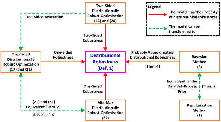
(a) Connections of Concepts Excluding Surrogates

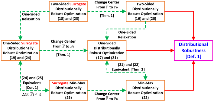
(b) Connections of Concepts Involving Surrogates. Model (25) is a formal definition of (and therefore the same as) Model (6).

Figure 2: Relations among concepts of distributional robustness, distributionally robust optimization method, Bayesian method, and regularization method.

Specifically, in terms of Figure 2(a), the relations can be summarized as follows.

1. The concept of distributional robustness is given in Definition 3.

2. Two-sided distributionally robust optimizations [i.e., (16) and (20)] and one-sided distributionally robust optimizations [i.e., (17) and (21)] can provide distributional robustness.

3. The difference between (16) and (20) is whether there is a condition $\Delta(\mathbb{P},\mathbb{P}_{0})\leq\epsilon$, so is between (17) and (21).

4. The one-sided distributionally robust optimization (21) is equivalent to a min-max distributionally robust optimization (22); see Theorem 12.

5. The Bayesian method (5) is probably approximately distributionally robust; see Theorem 19.

6. Under Dirichlet-process priors, the regularization method (7) is equivalent to a Bayesian method (5); see Theorem 20.

In terms of Figure 2(b), we have three more distributionally robust optimization models that work with the surrogate distribution $\bar{\mathbb{P}}$ instead of the true distribution $\mathbb{P}_{0}$. The relations can be summarized as follows.

1. By changing the center of the distributional family from $\bar{\mathbb{P}}$ to $\mathbb{P}_{0}$, the two-sided surrogate distributionally robust optimizations (18) and (23) can be transformed to the two-sided distributionally robust optimizations (16) and (20), respectively. The distributional robustness of the two-sided surrogate distributionally robust optimization (18) can be guaranteed by Theorem 8. The distributional robustness of the two-sided surrogate distributionally robust optimization (23) can be straightforwardly given in analogy to that of (18).

2. By changing the center of the distributional family from $\bar{\mathbb{P}}$ to $\mathbb{P}_{0}$, the one-sided surrogate distributionally robust optimizations (19) and (24) can be transformed to the one-sided distributionally robust optimizations (17) and (21), respectively. The distributional robustness of the one-sided surrogate distributionally robust optimization (19) can be guaranteed by Theorem 8. The distributional robustness of the one-sided surrogate distributionally robust optimization (24) can be straightforwardly given in analogy to that of (19).

3. The one-sided surrogate distributionally robust optimizations (19) and (24) are the one-sided relaxations of the two-sided surrogate distributionally robust optimizations (18) and (23), respectively.

4. The difference between (18) and (23) is whether there is a condition $\Delta(\mathbb{P},\bar{\mathbb{P}})\leq\epsilon$, so is between (19) and (24).

5. The one-sided surrogate distributionally robust optimization (24) is equivalent to a surrogate min-max distributionally robust optimization (25); see Corollary 16. Note that Model (25) is the formal definition of (and therefore the same as) Model (6).

Appendix B Proof of Proposition 36

Proof  Suppose $(\bm{x}^{*},\mathbb{P}^{*})$ solves (35). By Definition 35, we have

$$L^{*}\coloneqq\frac{|\mathbb{E}_{\mathbb{P}^{*}}h(\bm{x}^{*},\mathbf{\xi})-\mathbb{E}_{\mathbb{P}_{0}}h(\bm{x}_{0},\mathbf{\xi})|}{\Delta(\mathbb{P}^{*},\mathbb{P}_{0})}\geq\frac{|\mathbb{E}_{\mathbb{P}}h(\bm{x}^{*},\mathbf{\xi})-\mathbb{E}_{\mathbb{P}_{0}}h(\bm{x}_{0},\mathbf{\xi})|}{\Delta(\mathbb{P},\mathbb{P}_{0})},~{}~{}~{}~{}\forall\mathbb{P}\in\mathcal{M}(\Xi),$$

that is,

$$|\mathbb{E}_{\mathbb{P}}h(\bm{x}^{*},\mathbf{\xi})-\mathbb{E}_{\mathbb{P}_{0}}h(\bm{x}_{0},\mathbf{\xi})|\leq L^{*}\cdot\Delta(\mathbb{P},\mathbb{P}_{0}),~{}~{}~{}~{}\forall\mathbb{P}\in\mathcal{M}(\Xi).$$

Suppose $(\bm{x}^{*},L^{*})$ solves (16). We have

$$|\mathbb{E}_{\mathbb{P}}h(\bm{x}^{*},\mathbf{\xi})-\mathbb{E}_{\mathbb{P}_{0}}h(\bm{x}_{0},\mathbf{\xi})|\leq L^{*}\cdot\Delta(\mathbb{P},\mathbb{P}_{0}),~{}~{}~{}~{}\forall\mathbb{P}\in\mathcal{M}(\Xi).$$

As a result, by assuming that $\mathbb{P}^{*}$ satisfies the equality of the above display, we have

$$L^{*}=\frac{|\mathbb{E}_{\mathbb{P}^{*}}h(\bm{x}^{*},\mathbf{\xi})-\mathbb{E}_{\mathbb{P}_{0}}h(\bm{x}_{0},\mathbf{\xi})|}{\Delta(\mathbb{P}^{*},\mathbb{P}_{0})}\geq\frac{|\mathbb{E}_{\mathbb{P}}h(\bm{x}^{*},\mathbf{\xi})-\mathbb{E}_{\mathbb{P}_{0}}h(\bm{x}_{0},\mathbf{\xi})|}{\Delta(\mathbb{P},\mathbb{P}_{0})},~{}~{}~{}~{}\forall\mathbb{P}\in\mathcal{M}(\Xi).$$

This completes the proof. Note that two optimization problems are equivalent if an optimal solution of one optimization problem is a feasible solution of the other optimization problem. Note also that $\bm{x}^{*}$ and $\mathbb{P}^{*}$ may not be unique; however, this does not change the statement.  

Appendix C Proof of Theorem 8

Proof  We have, $\forall\mathbb{P}\in\mathcal{M}(\Xi)$,

$$\begin{array}[]{cl}|\mathbb{E}_{\mathbb{P}}h(\bm{x}_{1},\mathbf{\xi})-\mathbb{E}_{\mathbb{P}_{0}}h(\bm{x}_{0},\mathbf{\xi})|&=|\mathbb{E}_{\mathbb{P}}h(\bm{x}_{1},\mathbf{\xi})-\mathbb{E}_{\bar{\mathbb{P}}}h(\bar{\bm{x}},\mathbf{\xi})+\mathbb{E}_{\bar{\mathbb{P}}}h(\bar{\bm{x}},\mathbf{\xi})-\mathbb{E}_{\mathbb{P}_{0}}h(\bm{x}_{0},\mathbf{\xi})|\\ &\leq|\mathbb{E}_{\mathbb{P}}h(\bm{x}_{1},\mathbf{\xi})-\mathbb{E}_{\bar{\mathbb{P}}}h(\bar{\bm{x}},\mathbf{\xi})|+|\mathbb{E}_{\bar{\mathbb{P}}}h(\bar{\bm{x}},\mathbf{\xi})-\mathbb{E}_{\mathbb{P}_{0}}h(\bm{x}_{0},\mathbf{\xi})|\\ &\leq L_{1}\cdot\Delta(\mathbb{P},\bar{\mathbb{P}})+L_{2}\cdot\Delta(\bar{\mathbb{P}},\mathbb{P}_{0})\\ &\leq L\cdot\Delta(\mathbb{P},\mathbb{P}_{0}),\end{array}$$

where $L\coloneqq\max\{L_{1},L_{2}\}$.

Likewise, we have, $\forall\mathbb{P}\in\mathcal{M}(\Xi)$,

$$\begin{array}[]{cl}\mathbb{E}_{\mathbb{P}}h(\bm{x}_{1},\mathbf{\xi})-\mathbb{E}_{\mathbb{P}_{0}}h(\bm{x}_{0},\mathbf{\xi})&=\mathbb{E}_{\mathbb{P}}h(\bm{x}_{1},\mathbf{\xi})-\mathbb{E}_{\bar{\mathbb{P}}}h(\bar{\bm{x}},\mathbf{\xi})+\mathbb{E}_{\bar{\mathbb{P}}}h(\bar{\bm{x}},\mathbf{\xi})-\mathbb{E}_{\mathbb{P}_{0}}h(\bm{x}_{0},\mathbf{\xi})\\ &\leq\mathbb{E}_{\mathbb{P}}h(\bm{x}_{1},\mathbf{\xi})-\mathbb{E}_{\bar{\mathbb{P}}}h(\bar{\bm{x}},\mathbf{\xi})+|\mathbb{E}_{\bar{\mathbb{P}}}h(\bar{\bm{x}},\mathbf{\xi})-\mathbb{E}_{\mathbb{P}_{0}}h(\bm{x}_{0},\mathbf{\xi})|\\ &\leq L_{1}\cdot\Delta(\mathbb{P},\bar{\mathbb{P}})+L_{2}\cdot\Delta(\bar{\mathbb{P}},\mathbb{P}_{0})\\ &\leq L\cdot\Delta(\mathbb{P},\mathbb{P}_{0}).\end{array}$$

This completes the proof.  

Appendix D Proof of Theorem 12

Proof  By eliminating $L$, Problem (21) is equivalent to

$$\begin{array}[]{cl}\displaystyle\min_{\bm{x}}\max_{\mathbb{P}}&\displaystyle{\mathbb{E}_{\mathbb{P}}h(\bm{x},\mathbf{\xi})-\mathbb{E}_{\mathbb{P}_{0}}h(\bm{x}_{0},\mathbf{\xi})}\\ s.t.&\Delta(\mathbb{P},\mathbb{P}_{0})\leq\epsilon,\\ &\bm{x}\in\mathcal{X},\end{array}$$

which is further equivalent to (22) because $\mathbb{E}_{\mathbb{P}_{0}}h(\bm{x}_{0},\mathbf{\xi})$ is a constant. This completes the proof.  

Appendix E Proof of Theorem 18

Proof  We have

$$\begin{array}[]{cll}\mathbb{E}_{\mathbb{Q}}\mathbb{E}_{\mathbb{P}}h(\bm{x},\mathbf{\xi})\par&=\displaystyle\int_{\mathbb{R}}\cdot\int_{\Xi}h(\bm{x},\mathbf{\xi})\mathbb{P}(\mathrm{d}\mathbf{\xi})\cdot\mathbb{Q}(\mathrm{d}\mathbb{P}(\mathrm{d}\mathbf{\xi})),\\ &=\displaystyle\int_{\Xi}h(\bm{x},\mathbf{\xi})\cdot\int_{\mathbb{R}}\mathbb{P}(\mathrm{d}\mathbf{\xi})\mathbb{Q}(\mathrm{d}\mathbb{P}(\mathrm{d}\mathbf{\xi})),\\ &=\displaystyle\int_{\Xi}h(\bm{x},\mathbf{\xi})\bar{\mathbb{P}}(\mathrm{d}\mathbf{\xi}),\\ &=\mathbb{E}_{\bar{\mathbb{P}}}h(\bm{x},\mathbf{\xi}).\end{array}$$

The second equality is due to the measure-theoretic version of Fubini’s theorem (Cohn, 2013, p. 148) by noting that probability measures are $\sigma$-finite and that $\mathbb{P}(\mathrm{d}\mathbf{\xi})$ is a random variable on $\mathbb{R}$ for every Borel set $\mathrm{d}\mathbf{\xi}$. The third equality is due to the definition of a mean distribution by noting that the mean distribution of $\mathbb{Q}$ is essentially a mixture distribution of the elements in the set $\mathcal{M}(\Xi)$ with weights determined by $\mathbb{Q}$; cf. Gaudard and Hadwin (1989), Ghosal and Van der Vaart (2017, p. 27).  

Appendix F Proof of Theorem 20

Proof  If (32) holds, the associated regularized SAA optimization problem (31) is equivalent to a Bayesian method (29). By constructing the posterior mean of $\mathbb{Q}$ to be $\mathbb{E}\mathbb{Q}\coloneqq\beta_{n}\hat{\mathbb{P}}+(1-\beta_{n})\hat{\mathbb{P}}_{n}$, we have that (31) is equivalent to (5). The rest of the statement follows from Markov’s inequality; cf. Theorem 19 and its proof.  

Appendix G Proof of Proposition 24

Proof  We have

$$\begin{array}[]{cl}|\mathbb{E}_{\mathbb{P}_{0}}h(\bm{x},\mathbf{\xi})-\mathbb{E}_{\bar{\mathbb{P}}}h(\bm{x},\mathbf{\xi})|&=\displaystyle\left|\int\int h(\bm{x},\mathbf{\xi})-h(\bm{x},\bar{\mathbf{\xi}})\mathrm{d}\pi(\mathbf{\xi},\bar{\mathbf{\xi}})\right|\\ &\leq\displaystyle\int\int\Big{|}h(\bm{x},\mathbf{\xi})-h(\bm{x},\bar{\mathbf{\xi}})\Big{|}\mathrm{d}\pi(\mathbf{\xi},\bar{\mathbf{\xi}})\\ &\leq L(\bm{x})\displaystyle\int\int\|\mathbf{\xi}-\bar{\mathbf{\xi}}\|\mathrm{d}\pi(\mathbf{\xi},\bar{\mathbf{\xi}}),\end{array}$$

where $\pi$ is a coupling of $\mathbb{P}_{0}$ and $\bar{\mathbb{P}}$. Since $\pi$ is arbitrary, it holds that

$$|\mathbb{E}_{\mathbb{P}_{0}}h(\bm{x},\mathbf{\xi})-\mathbb{E}_{\bar{\mathbb{P}}}h(\bm{x},\mathbf{\xi})|\leq L(\bm{x})\displaystyle\inf_{\pi\in\mathcal{M}(\Xi\times\Xi)}\int\int\|\mathbf{\xi}-\bar{\mathbf{\xi}}\|\mathrm{d}\pi(\mathbf{\xi},\bar{\mathbf{\xi}}).$$

The right-hand side is the order-$1$ Wasserstein distance. This completes the proof.  

Appendix H Proof of Theorem 27

Proof  Due to the feasibility of $(\bm{x}^{*},L^{*},\mathbb{P}_{0})$, we have

$$|\mathbb{E}_{\mathbb{P}_{0}}h(\bm{x}^{*},\mathbf{\xi})-\mathbb{E}_{\bar{\mathbb{P}}}h(\bar{\bm{x}},\mathbf{\xi})|\leq L^{*}.$$

Hence, if $h(\bm{x},\mathbf{\xi})$ is $L(\mathbf{\xi})$-Lipschitz continuous in $\bm{x}$ on $\mathcal{X}$, the generalization error $|\mathbb{E}_{\mathbb{P}_{0}}h(\bar{\bm{x}},\mathbf{\xi})-\mathbb{E}_{\bar{\mathbb{P}}}h(\bar{\bm{x}},\mathbf{\xi})|$ of the nominal model $\min_{\bm{x}}\mathbb{E}_{\bar{\mathbb{P}}}h(\bm{x},\mathbf{\xi})$ can be given as

$$\begin{array}[]{cl}|\mathbb{E}_{\mathbb{P}_{0}}h(\bar{\bm{x}},\mathbf{\xi})-\mathbb{E}_{\bar{\mathbb{P}}}h(\bar{\bm{x}},\mathbf{\xi})|&=|\mathbb{E}_{\mathbb{P}_{0}}h(\bar{\bm{x}},\mathbf{\xi})-\mathbb{E}_{\mathbb{P}_{0}}h(\bm{x}^{*},\mathbf{\xi})+\mathbb{E}_{\mathbb{P}_{0}}h(\bm{x}^{*},\mathbf{\xi})-\mathbb{E}_{\bar{\mathbb{P}}}h(\bar{\bm{x}},\mathbf{\xi})|\\ &\leq|\mathbb{E}_{\mathbb{P}_{0}}h(\bar{\bm{x}},\mathbf{\xi})-\mathbb{E}_{\mathbb{P}_{0}}h(\bm{x}^{*},\mathbf{\xi})|+|\mathbb{E}_{\mathbb{P}_{0}}h(\bm{x}^{*},\mathbf{\xi})-\mathbb{E}_{\bar{\mathbb{P}}}h(\bar{\bm{x}},\mathbf{\xi})|\\ &\leq\mathbb{E}_{\mathbb{P}_{0}}|h(\bar{\bm{x}},\mathbf{\xi})-h(\bm{x}^{*},\mathbf{\xi})|+L^{*}\\ &\leq\|\bar{\bm{x}}-\bm{x}^{*}\|\cdot\mathbb{E}_{\mathbb{P}_{0}}L(\mathbf{\xi})+L^{*}.\end{array}$$

The above display holds $\mathbb{P}^{n}_{0}$-almost surely. Similarly, since $|\mathbb{E}_{\mathbb{P}^{*}}h(\bm{x}^{*},\mathbf{\xi})-\mathbb{E}_{\bar{\mathbb{P}}}h(\bar{\bm{x}},\mathbf{\xi})|=L^{*}$, we have

$$\begin{array}[]{cl}|\mathbb{E}_{\mathbb{P}_{0}}h(\bm{x}^{*},\mathbf{\xi})-\mathbb{E}_{\mathbb{P}^{*}}h(\bm{x}^{*},\mathbf{\xi})|&\leq|\mathbb{E}_{\mathbb{P}_{0}}h(\bm{x}^{*},\mathbf{\xi})-\mathbb{E}_{\bar{\mathbb{P}}}h(\bar{\bm{x}},\mathbf{\xi})|+|\mathbb{E}_{\mathbb{P}^{*}}h(\bm{x}^{*},\mathbf{\xi})-\mathbb{E}_{\bar{\mathbb{P}}}h(\bar{\bm{x}},\mathbf{\xi})|\\ &\leq L^{*}+L^{*}=2L^{*}.\end{array}$$

The above display holds $\mathbb{P}^{n}_{0}$-almost surely. This completes the proof.  

Appendix I Proof of Corollary 29

Proof  We have

$$\begin{array}[]{cl}\mathbb{E}_{\mathbb{P}^{n}_{0}}|\mathbb{E}_{\mathbb{P}_{0}}h(\bar{\bm{x}},\mathbf{\xi})-\mathbb{E}_{\bar{\mathbb{P}}}h(\bar{\bm{x}},\mathbf{\xi})|&=\mathbb{E}_{\mathbb{P}^{n}_{0}}|\mathbb{E}_{\mathbb{P}_{0}}h(\bar{\bm{x}},\mathbf{\xi})-\mathbb{E}_{\mathbb{P}_{0}}h(\bm{x}^{*},\mathbf{\xi})+\mathbb{E}_{\mathbb{P}_{0}}h(\bm{x}^{*},\mathbf{\xi})-\mathbb{E}_{\bar{\mathbb{P}}}h(\bar{\bm{x}},\mathbf{\xi})|\\ &\leq\mathbb{E}_{\mathbb{P}^{n}_{0}}|\mathbb{E}_{\mathbb{P}_{0}}h(\bar{\bm{x}},\mathbf{\xi})-\mathbb{E}_{\mathbb{P}_{0}}h(\bm{x}^{*},\mathbf{\xi})|+\mathbb{E}_{\mathbb{P}^{n}_{0}}|\mathbb{E}_{\mathbb{P}_{0}}h(\bm{x}^{*},\mathbf{\xi})-\mathbb{E}_{\bar{\mathbb{P}}}h(\bar{\bm{x}},\mathbf{\xi})|\\ &\leq\mathbb{E}_{\mathbb{P}_{0}^{n+1}}|h(\bar{\bm{x}},\mathbf{\xi})-h(\bm{x}^{*},\mathbf{\xi})|+\mathbb{E}_{\mathbb{P}^{n}_{0}}L^{*}\\ &\leq\mathbb{E}_{\mathbb{P}_{0}^{n+1}}L(\mathbf{\xi})\|\bar{\bm{x}}-\bm{x}^{*}\|+\mathbb{E}_{\mathbb{P}^{n}_{0}}L^{*}.\end{array}$$

The other statement is obvious. This completes the proof.  

Appendix J Proof of Theorem 30

Proof  The relative robustness measure $L^{*}$ of the solution $\bm{x}^{*}$ satisfies

$$|\mathbb{E}_{\mathbb{P}_{0}}h(\bm{x}^{*},\mathbf{\xi})-\mathbb{E}_{\bar{\mathbb{P}}}h(\bar{\bm{x}},\mathbf{\xi})|\leq L^{*}\Delta(\mathbb{P}_{0},\bar{\mathbb{P}}).$$

Hence, if $h(\bm{x},\mathbf{\xi})$ is $L(\mathbf{\xi})$-Lipschitz continuous in $\bm{x}$ on $\mathcal{X}$, the generalization error $|\mathbb{E}_{\mathbb{P}_{0}}h(\bar{\bm{x}},\mathbf{\xi})-\mathbb{E}_{\bar{\mathbb{P}}}h(\bar{\bm{x}},\mathbf{\xi})|$ of the nominal model $\min_{\bm{x}}\mathbb{E}_{\bar{\mathbb{P}}}h(\bm{x},\mathbf{\xi})$ can be given as

$$\begin{array}[]{cl}|\mathbb{E}_{\mathbb{P}_{0}}h(\bar{\bm{x}},\mathbf{\xi})-\mathbb{E}_{\bar{\mathbb{P}}}h(\bar{\bm{x}},\mathbf{\xi})|&=|\mathbb{E}_{\mathbb{P}_{0}}h(\bar{\bm{x}},\mathbf{\xi})-\mathbb{E}_{\mathbb{P}_{0}}h(\bm{x}^{*},\mathbf{\xi})+\mathbb{E}_{\mathbb{P}_{0}}h(\bm{x}^{*},\mathbf{\xi})-\mathbb{E}_{\bar{\mathbb{P}}}h(\bar{\bm{x}},\mathbf{\xi})|\\ &\leq|\mathbb{E}_{\mathbb{P}_{0}}h(\bar{\bm{x}},\mathbf{\xi})-\mathbb{E}_{\mathbb{P}_{0}}h(\bm{x}^{*},\mathbf{\xi})|+|\mathbb{E}_{\mathbb{P}_{0}}h(\bm{x}^{*},\mathbf{\xi})-\mathbb{E}_{\bar{\mathbb{P}}}h(\bar{\bm{x}},\mathbf{\xi})|\\ &\leq\mathbb{E}_{\mathbb{P}_{0}}|h(\bar{\bm{x}},\mathbf{\xi})-h(\bm{x}^{*},\mathbf{\xi})|+L^{*}\Delta(\mathbb{P}_{0},\bar{\mathbb{P}})\\ &\leq\mathbb{E}_{\mathbb{P}_{0}}L(\mathbf{\xi})\|\bar{\bm{x}}-\bm{x}^{*}\|+L^{*}\Delta(\mathbb{P}_{0},\bar{\mathbb{P}}).\end{array}$$

The above display holds $\mathbb{P}^{n}_{0}$-almost surely. Similarly, since $|\mathbb{E}_{\mathbb{P}^{*}}h(\bm{x}^{*},\mathbf{\xi})-\mathbb{E}_{\bar{\mathbb{P}}}h(\bar{\bm{x}},\mathbf{\xi})|=L^{*}\Delta(\bar{\mathbb{P}},\mathbb{P}^{*})$, we have

$$\begin{array}[]{cl}|\mathbb{E}_{\mathbb{P}_{0}}h(\bm{x}^{*},\mathbf{\xi})-\mathbb{E}_{\mathbb{P}^{*}}h(\bm{x}^{*},\mathbf{\xi})|&\leq|\mathbb{E}_{\mathbb{P}_{0}}h(\bm{x}^{*},\mathbf{\xi})-\mathbb{E}_{\bar{\mathbb{P}}}h(\bar{\bm{x}},\mathbf{\xi})|+|\mathbb{E}_{\mathbb{P}^{*}}h(\bm{x}^{*},\mathbf{\xi})-\mathbb{E}_{\bar{\mathbb{P}}}h(\bar{\bm{x}},\mathbf{\xi})|\\ &\leq L^{*}\Delta(\mathbb{P}_{0},\bar{\mathbb{P}})+L^{*}\Delta(\mathbb{P}^{*},\bar{\mathbb{P}})\\ &\leq L^{*}\Delta(\mathbb{P}_{0},\mathbb{P}^{*}).\end{array}$$

The above display holds $\mathbb{P}^{n}_{0}$-almost surely. This completes the proof.  

Appendix K Proof of Corollary 31

Proof  We have

$$\begin{array}[]{cl}\mathbb{E}_{\mathbb{P}^{n}_{0}}|\mathbb{E}_{\mathbb{P}_{0}}h(\bar{\bm{x}},\mathbf{\xi})-\mathbb{E}_{\bar{\mathbb{P}}}h(\bar{\bm{x}},\mathbf{\xi})|&=\mathbb{E}_{\mathbb{P}^{n}_{0}}|\mathbb{E}_{\mathbb{P}_{0}}h(\bar{\bm{x}},\mathbf{\xi})-\mathbb{E}_{\mathbb{P}_{0}}h(\bm{x}^{*},\mathbf{\xi})+\mathbb{E}_{\mathbb{P}_{0}}h(\bm{x}^{*},\mathbf{\xi})-\mathbb{E}_{\bar{\mathbb{P}}}h(\bar{\bm{x}},\mathbf{\xi})|\\ &\leq\mathbb{E}_{\mathbb{P}^{n}_{0}}|\mathbb{E}_{\mathbb{P}_{0}}h(\bar{\bm{x}},\mathbf{\xi})-\mathbb{E}_{\mathbb{P}_{0}}h(\bm{x}^{*},\mathbf{\xi})|+\mathbb{E}_{\mathbb{P}^{n}_{0}}|\mathbb{E}_{\mathbb{P}_{0}}h(\bm{x}^{*},\mathbf{\xi})-\mathbb{E}_{\bar{\mathbb{P}}}h(\bar{\bm{x}},\mathbf{\xi})|\\ &\leq\mathbb{E}_{\mathbb{P}_{0}^{n+1}}|h(\bar{\bm{x}},\mathbf{\xi})-h(\bm{x}^{*},\mathbf{\xi})|+\mathbb{E}_{\mathbb{P}^{n}_{0}}L^{*}\Delta(\mathbb{P}_{0},\bar{\mathbb{P}})\\ &\leq\mathbb{E}_{\mathbb{P}_{0}^{n+1}}L(\mathbf{\xi})\|\bar{\bm{x}}-\bm{x}^{*}\|+\mathbb{E}_{\mathbb{P}^{n}_{0}}L^{*}\Delta(\mathbb{P}_{0},\bar{\mathbb{P}}).\end{array}$$

The other statement is obvious. This completes the proof.

References

- Anderson and Moore (1979) Brian DO Anderson and John B Moore. Optimal Filtering. Courier Corporation, 1979.
- Anderson and Nguyen (2020) Edward Anderson and Harrison Nguyen. When can we improve on sample average approximation for stochastic optimization? Operations Research Letters, 48(5):566–572, 2020.
- Ben-Tal et al. (2013) Aharon Ben-Tal, Dick Den Hertog, Anja De Waegenaere, Bertrand Melenberg, and Gijs Rennen. Robust solutions of optimization problems affected by uncertain probabilities. Management Science, 59(2):341–357, 2013.
- Bertsimas and Copenhaver (2018) Dimitris Bertsimas and Martin S Copenhaver. Characterization of the equivalence of robustification and regularization in linear and matrix regression. European Journal of Operational Research, 270(3):931–942, 2018.
- Billingsley (1999) Patrick Billingsley. Convergence of Probability Measures. John Wiley & Sons, 2 edition, 1999.
- Bishop and Nasrabadi (2006) Christopher M Bishop and Nasser M Nasrabadi. Pattern Recognition and Machine Learning. Springer, 2006.
- Blanchet et al. (2019) Jose Blanchet, Yang Kang, and Karthyek Murthy. Robust Wasserstein profile inference and applications to machine learning. Journal of Applied Probability, 56(3):830–857, 2019.
- Blanchet et al. (2021) Jose Blanchet, Lin Chen, and Xun Yu Zhou. Distributionally robust mean-variance portfolio selection with Wasserstein distances. Management Science, 2021.
- Bousquet and Elisseeff (2002) Olivier Bousquet and André Elisseeff. Stability and generalization. The Journal of Machine Learning Research, 2:499–526, 2002.
- Brownlees et al. (2015) Christian Brownlees, Emilien Joly, and Gábor Lugosi. Empirical risk minimization for heavy-tailed losses. The Annals of Statistics, 43(6):2507–2536, 2015.
- Chen et al. (2020) Ruidi Chen, Ioannis Ch Paschalidis, et al. Distributionally robust learning. Foundations and Trends® in Optimization, 4(1-2):1–243, 2020.
- Cohn (2013) Donald L Cohn. Measure Theory, volume 1. Springer, 2 edition, 2013.
- Domingos (2012) Pedro Domingos. A few useful things to know about machine learning. Communications of the ACM, 55(10):78–87, 2012.
- Duchi et al. (2021) John C Duchi, Peter W Glynn, and Hongseok Namkoong. Statistics of robust optimization: A generalized empirical likelihood approach. Mathematics of Operations Research, 46(3):946–969, 2021.
- Ferguson (1973) Thomas S Ferguson. A Bayesian analysis of some nonparametric problems. The Annals of Statistics, pages 209–230, 1973.
- Fournier and Guillin (2015) Nicolas Fournier and Arnaud Guillin. On the rate of convergence in Wasserstein distance of the empirical measure. Probability Theory and Related Fields, 162(3):707–738, 2015.
- Gao (2022) Rui Gao. Finite-sample guarantees for Wasserstein distributionally robust optimization: Breaking the curse of dimensionality. Operations Research, 2022.
- Gao and Kleywegt (2022) Rui Gao and Anton Kleywegt. Distributionally robust stochastic optimization with Wasserstein distance. Mathematics of Operations Research, 2022.
- Gao et al. (2022) Rui Gao, Xi Chen, and Anton J Kleywegt. Wasserstein distributionally robust optimization and variation regularization. Operations Research, 2022.
- Gaudard and Hadwin (1989) Marie Gaudard and Donald Hadwin. Sigma-algebras on spaces of probability measures. Scandinavian Journal of Statistics, pages 169–175, 1989.
- Germain et al. (2009) Pascal Germain, Alexandre Lacasse, François Laviolette, and Mario Marchand. PAC-Bayesian learning of linear classifiers. In Proceedings of the 26th Annual International Conference on Machine Learning, pages 353–360, 2009.
- Germain et al. (2016) Pascal Germain, Francis Bach, Alexandre Lacoste, and Simon Lacoste-Julien. PAC-Bayesian theory meets Bayesian inference. Advances in Neural Information Processing Systems, 29, 2016.
- Ghosal and Van der Vaart (2017) Subhashis Ghosal and Aad Van der Vaart. Fundamentals of Nonparametric Bayesian Inference, volume 44. Cambridge University Press, 2017.
- Givens and Shortt (1984) Clark R Givens and Rae Michael Shortt. A class of Wasserstein metrics for probability distributions. Michigan Mathematical Journal, 31(2):231–240, 1984.
- Goodfellow et al. (2016) Ian Goodfellow, Yoshua Bengio, and Aaron Courville. Deep Learning. MIT Press, 2016.
- Gotoh et al. (2018) Jun-Ya Gotoh, Michael Jong Kim, and Andrew EB Lim. Robust empirical optimization is almost the same as mean–variance optimization. Operations Research Letters, 46(4):448–452, 2018.
- Gotoh et al. (2021) Jun-Ya Gotoh, Michael Jong Kim, and Andrew EB Lim. Calibration of distributionally robust empirical optimization models. Operations Research, 69(5):1630–1650, 2021.
- Hampel (1974) Frank R Hampel. The influence curve and its role in robust estimation. Journal of the American Statistical Association, 69(346):383–393, 1974.
- Hassibi et al. (1996) Babak Hassibi, Ali H Sayed, and Thomas Kailath. Linear estimation in Krein spaces. i. theory. IEEE Transactions on Automatic Control, 41(1):18–33, 1996.
- Hastie et al. (2009) Trevor Hastie, Robert Tibshirani, and Jerome Friedman. The elements of statistical learning: Data mining, inference, and prediction. Springer New York, 2009.
- Huber (1964) Peter J. Huber. Robust estimation of a location parameter. The Annals of Mathematical Statistics, 35(1):73–101, 1964.
- Huber and Ronchetti (2009) Peter J. Huber and eauthor Ronchetti, Elvezio M. Robust Statistics. Wiley, 2 edition, 2009.
- James et al. (2021) Gareth James, Daniela Witten, Trevor Hastie, and Robert Tibshirani. An Introduction to Statistical Learning. Springer, 2 edition, 2021.
- Kuhn et al. (2019) Daniel Kuhn, Peyman Mohajerin Esfahani, Viet Anh Nguyen, and Soroosh Shafieezadeh-Abadeh. Wasserstein distributionally robust optimization: Theory and applications in machine learning. In Operations Research & Management Science in the Age of Analytics, pages 130–166. Informs, 2019.
- Long et al. (2022) Daniel Zhuoyu Long, Melvyn Sim, and Minglong Zhou. Robust satisficing. Operations Research, 2022.
- Mohajerin Esfahani and Kuhn (2018) Peyman Mohajerin Esfahani and Daniel Kuhn. Data-driven distributionally robust optimization using the Wasserstein metric: Performance guarantees and tractable reformulations. Mathematical Programming, 171(1):115–166, 2018.
- Mohri et al. (2018) Mehryar Mohri, Afshin Rostamizadeh, and Ameet Talwalkar. Foundations of Machine Learning. MIT Press, 2018.
- Murphy (2012) Kevin P Murphy. Machine Learning: A Probabilistic Perspective. MIT Press, 2012.
- Rahimian and Mehrotra (2022) Hamed Rahimian and Sanjay Mehrotra. Frameworks and results in distributionally robust optimization. Open Journal of Mathematical Optimization, 3:1–85, 2022.
- Rodríguez Gálvez et al. (2021) Borja Rodríguez Gálvez, Germán Bassi, Ragnar Thobaben, and Mikael Skoglund. Tighter expected generalization error bounds via Wasserstein distance. Advances in Neural Information Processing Systems, 34:19109–19121, 2021.
- Römisch and Schultz (1991) Werner Römisch and Rüdiger Schultz. Stability analysis for stochastic programs. Annals of Operations Research, 30(1):241–266, 1991.
- Shafieezadeh-Abadeh et al. (2019) Soroosh Shafieezadeh-Abadeh, Daniel Kuhn, and Peyman Mohajerin Esfahani. Regularization via mass transportation. Journal of Machine Learning Research, 20(103):1–68, 2019.
- Shapiro (2017) Alexander Shapiro. Distributionally robust stochastic programming. SIAM Journal on Optimization, 27(4):2258–2275, 2017.
- Shapiro et al. (2009) Alexander Shapiro, Darinka Dentcheva, and Andrzej Ruszczynski. Lectures on Stochastic Programming: Modeling and Theory. SIAM, 2009.
- Sun and Xu (2016) Hailin Sun and Huifu Xu. Convergence analysis for distributionally robust optimization and equilibrium problems. Mathematics of Operations Research, 41(2):377–401, 2016.
- Tang and Qian (2010) Qi Tang and Peter ZG Qian. Enhancing the sample average approximation method with u designs. Biometrika, 97(4):947–960, 2010.
- Van der Vaart (2000) A. W. Van der Vaart. Asymptotic Statistics. Cambridge University Press, 2000.
- Van der Vaart and Wellner (1996) A. W. Van der Vaart and Jon A Wellner. Weak Convergence and Empirical Processes. Springer, 1996.
- Van Parys et al. (2015) Bart PG Van Parys, Daniel Kuhn, Paul J Goulart, and Manfred Morari. Distributionally robust control of constrained stochastic systems. IEEE Transactions on Automatic Control, 61(2):430–442, 2015.
- Van Parys et al. (2021) Bart PG Van Parys, Peyman Mohajerin Esfahani, and Daniel Kuhn. From data to decisions: Distributionally robust optimization is optimal. Management Science, 67(6):3387–3402, 2021.
- Vapnik (1998) Vladimir Vapnik. Statistical Learning Theory. Wiley-Interscience, 1998.
- Vapnik (2000) Vladimir Vapnik. The Nature of Statistical Learning Theory. Springer, 2 edition, 2000.
- Wainwright (2019) Martin J Wainwright. High-Dimensional Statistics: A Non-Asymptotic Viewpoint, volume 48. Cambridge University Press, 2019.
- Wang et al. (2019) Hao Wang, Mario Diaz, José Cândido S Santos Filho, and Flavio P Calmon. An information-theoretic view of generalization via Wasserstein distance. In 2019 IEEE International Symposium on Information Theory (ISIT), pages 577–581. IEEE, 2019.
- Wang et al. (2022) Qi Wang, Yue Ma, Kun Zhao, and Yingjie Tian. A comprehensive survey of loss functions in machine learning. Annals of Data Science, 9(2):187–212, 2022.
- Wang (2022a) Shixiong Wang. Distributionally robust state estimation for nonlinear systems. IEEE Transactions on Signal Processing, 70:4408–4423, 2022a.
- Wang (2022b) Shixiong Wang. Distributionally Robust State Estimation. PhD thesis, National University of Singapore, 1 2022b.
- Weed and Bach (2019) Jonathan Weed and Francis Bach. Sharp asymptotic and finite-sample rates of convergence of empirical measures in Wasserstein distance. Bernoulli, 25(4A):2620–2648, 2019.
- Wu et al. (2018) Di Wu, Helin Zhu, and Enlu Zhou. A Bayesian risk approach to data-driven stochastic optimization: Formulations and asymptotics. SIAM Journal on Optimization, 28(2):1588–1612, 2018.
- Xu and Raginsky (2017) Aolin Xu and Maxim Raginsky. Information-theoretic analysis of generalization capability of learning algorithms. Advances in Neural Information Processing Systems, 30, 2017.
- Yue et al. (2021) Man-Chung Yue, Daniel Kuhn, and Wolfram Wiesemann. On linear optimization over Wasserstein balls. Mathematical Programming, pages 1–16, 2021.
- Zhang and Chen (2021) Huiming Zhang and Songxi Chen. Concentration inequalities for statistical inference. Communications in Mathematical Research, 37(1):1–85, 2021.
- Zhang et al. (2022) Luhao Zhang, Jincheng Yang, and Rui Gao. A simple duality proof for Wasserstein distributionally robust optimization. arXiv preprint arXiv:2205.00362, 2022.