The pressure-wired Stokes element: a mesh-robust version of the Scott-Vogelius element

Abstract

The Scott-Vogelius finite element pair for the numerical discretization of the stationary Stokes equation in 2D is a popular element which is based on a continuous velocity approximation of polynomial order $k$ and a discontinuous pressure approximation of order $k-1$. It employs a “singular distance” (measured by some geometric mesh quantity $\Theta\left(\mathbf{z}\right)\geq 0$ for triangle vertices $\mathbf{z}$) and imposes a local side condition on the pressure space associated to vertices $\mathbf{z}$ with $\Theta\left(\mathbf{z}\right)=0$. The method is inf-sup stable for any fixed regular triangulation and $k\geq 4$. However, the inf-sup constant deteriorates if the triangulation contains nearly singular vertices $0<\Theta\left(\mathbf{z}\right)\ll 1$.

In this paper, we introduce a very simple parameter-dependent modification of the Scott-Vogelius element such that the inf-sup constant is independent of nearly-singular vertices. We will show by analysis and also by numerical experiments that the effect on the divergence-free condition for the discrete velocity is negligibly small.

MSC Classification]65N30, 65N12, 76D07

1 Introduction

In this paper we consider the numerical solution of the stationary Stokes equation in a bounded two-dimensional polygonal Lipschitz domain by a conforming Galerkin finite element method.

Motivation. The intuitive choice for a Stokes element $\left(\mathbf{S}_{k}\left(\mathcal{T}\right),\mathbb{P}_{k-1}\left(\mathcal{T}\right)\right)$, where $\mathbf{S}_{k}\left(\mathcal{T}\right)$ denotes the space of continuous velocity fields with local polynomial degree $k$ over a given triangulation $\mathcal{T}$ and $\mathbb{P}_{k-1}\left(\mathcal{T}\right)$ the discontinuous pressures space of degree $k-1$, is in general not inf-sup stable (see, e.g., [1] and [2, Chap. 7] for quadrilateral meshes). A careful analysis [1], [3] of the range of the divergence operator reveals that the image $\operatorname{div}(\mathbf{S}_{k}(\mathcal{T}))\subset\mathbb{P}_{k-1}(\mathcal{T})$ reduces by one linear constraint for every singular vertex. For $k\geq 4$, this results in the inf-sup stable Scott-Vogelius [3] pair $(\mathbf{S}_{k}(\mathcal{T}),\operatorname{div}(\mathbf{S}_{k}(\mathcal{T})))$ on families of shape-regular meshes [4] that naturally computes fully divergence-free velocity approximations. However the Scott-Vogelius element, as described in [1], [3] and [4], has two major drawbacks.

1. The inf-sup constant is not robust with respect to small perturbations of the mesh when a singular vertex becomes nearly singular, measured through the geometric quantity $\Theta_{\min}:=\left\{\left.\Theta\left(\mathbf{z}\right)\;\right|\;\Theta\left(\mathbf{z}\right)>0\right\}$. Here $\Theta\left(\mathbf{z}\right)$ is a measure of the singular distance of a vertex $\mathbf{z}$ from a proper singular situation. The geometric quantity $\Theta_{\min}$ strongly affects the stability of the discretization, the size of the discretization error, as well as the condition number of the resulting algebraic linear system.

2. In order to implement the method, the condition: “Is a mesh point, say $\mathbf{z}$, a singular vertex?” cannot be realized in floating point arithmetics and has to be replaced by a threshold condition for “nearly singular vertices” of the form “$\Theta\left(\mathbf{z}\right)\leq\varepsilon$”. Through this threshold condition, it is possible that the constraints are imposed on nearly singular vertices, i.e. for ${0}<\Theta\left(\mathbf{z}\right)\leq\varepsilon$ and the discrete velocity looses the divergence-free property as a consequence. To the best of our knowledge, this effect has not been analyzed in the literature and we will estimate the influence of $\varepsilon>0$ to the divergence-free property of the discrete velocity in Section 5.

In [5, Rem.  2], two mesh modification strategies are sketched as a remedy of (1): i) nearly singular vertices are moved so that they become properly singular; ii) triangles which contain a nearly singular vertex are refined. Both strategies require the finite element code to have control on the mesh generator which is not realistic in many engineering applications and might also be in conflict with the solver for the linear system.

In this paper, we propose a simpler strategy where a modification of the mesh is avoided. We introduce a parameter dependent modification to the standard Scott-Vogelius pair, the pressure-wired Stokes element, and prove that the inf-sup constant is independent of $\Theta_{\min}$, the mesh width, the polynomial degree but depends only on the shape-regularity of the mesh.

Main Contributions. The construction of our modification employs a geometric quantity $\Theta\left(\mathbf{z}\right)\geq 0$ which measures the singular distance of the vertex $\mathbf{z}$ in the mesh from a singular configuration. For some arbitrary (in general small) control parameter $0\leq\eta$, the pressure space is reduced by the same constraint as in the Scott-Vogelius FEM for every vertex with singular distance $\Theta(\mathbf{z})\leq\eta$, which we call nearly singular. Since the constraints involve the sum of pressure values over all triangles that encircle a nearly singular vertex we call the new element the pressure-wired Stokes element. The proof that the inf-sup constant of this element is independent of the mesh width, the polynomial degree, and depends on the mesh only via the shape-regularity constant will be based on the results in [5, Sections 4 & 5], where the discrete stability of the pressure-wired Stokes element is proved via a lower bound for the inf-sup constant of the form $c\Theta_{\min}>0$ with a positive constant $c$ only depending on the domain and the shape regularity. We can therefore choose the threshold $\eta$ for our generalization of the Scott-Vogelius element such that the resulting pressure wired Stokes element is inf-sup stable independent of the mesh size, the polynomial degree, and any (nearly) singular vertex and that mitigates the drawbacks of the Scott-Vogelius pair mentioned above. These improvements come at some cost: in general we cannot expect divergence-free velocity approximations as for the standard Scott-Vogelius pair. We investigate the dependence of the $L^{2}$ norm of the divergence of the velocity approximation $\mathbf{u}_{\mathbf{S}}$ in the pressure-wired Stokes element and establish an estimate of the form $\left\|\operatorname{div}\mathbf{u}_{\mathbf{S}}\right\|_{L^{2}\left(\Omega\right)}\leq C\eta$ with $C>0$ being independent of the mesh width and the polynomial degree. We emphasize that this estimate does not require any regularity of the Stokes problem. Numerical experiments will be reported in Section 6 and show that the constant $C$ is very small for the considered examples.

Literature overview. Our pressure-wired Stokes element places few additional constraints on the pressure space to acquire robust inf-sup stability on arbitrary shape-regular grids – the proof for the estimate of the inf-sup constant is based on the theory developed in [1], [6], [3], [4], [7], [5]. An alternative approach constitutes the enrichment of the velocity space, e.g., in [8] with Raviart-Thomas bubble functions leading to a divergence-free velocity approximation in $H(\operatorname{div})$. Conforming alternatives to the Scott-Vogelius element are the Mini element [9], the (modified) Taylor-Hood element [2, Chap. 3, §7], the Bernardi-Raugel element [6], and the element by Falk-Neilan [10] to mention some but few of them. We note that there exist further possibilities to obtain a stable discretization of the Stokes equation; one is the use of non-conforming schemes and/or modifications of the discrete equation by adding stabilizing terms. We do not go into details here but refer to the monographs and overviews [11], [12], [13] instead.

Further contributions and outline: After introducing the Stokes problem on the continuous as well as on the discrete level and the relevant notation in Section 2, we define the conforming pressure-wired Stokes element in Section 3. The first main result in Section 4 establishes the discrete inf-sup condition for this new element with a lower bound on the inf-sup constant that is independent of $h,k$, and (nearly) critical points. The second main result controls the $L^{2}$ norm of the divergence of the discrete velocity in Section 5 and verifies its negligibility for small $\eta\ll 1$ in practice. In fact, the $L^{2}$ norm tends to zero (at least) linearly in $\eta$ without imposing any regularity assumption on the continuous problem. The involved constants are again independent of $h$, $k$, and $\Theta_{\min}$ but possibly depend on the mesh via its shape-regularity constant. We report on numerical evidence on optimal convergence rates in Section 6, both as an $h$-version with regular mesh refinement and as a $k$-version that successively increases the polynomial degree. While this new element is technically not divergence-free, our benchmarks suggest that the discrete divergence is near machine-precision already on coarse meshes and for moderate parameters $\eta>0$.

2 The Stokes problem and its numerical discretization

Let $\Omega\subset\mathbb{R}^{2}$ denote a bounded polygonal Lipschitz domain with boundary $\partial\Omega$. We consider the numerical solution of the Stokes equation

$$\begin{array}[]{lll}-\Delta\mathbf{u}+\nabla p&=\mathbf{f}&\text{in }\Omega,\\ \operatorname{div}\mathbf{u}&=0&\text{in }\Omega\end{array}$$

with homogeneous Dirichlet boundary conditions for the velocity and the usual normalisation condition for the pressure

$$\mathbf{u}=\mathbf{0}\quad\text{on }\partial\Omega\quad\text{and\quad}\int_{\Omega}p=0.$$

Throughout this paper standard notation for Lebesgue and Sobolev spaces applies. All function spaces are considered over the field of real numbers. The space $H_{0}^{1}\left(\Omega\right)$ is the closure of the space of smooth functions with compact support in $\Omega$ with respect to the $H^{1}\left(\Omega\right)$ norm. Its dual space is denoted by $H^{-1}\left(\Omega\right):=H_{0}^{1}\left(\Omega\right)^{\prime}$. The scalar product and norm in $L^{2}\left(\Omega\right)$ read

$$\left(u,v\right)_{L^{2}\left(\Omega\right)}:=\int_{\Omega}uv\quad\text{and}\quad\left\|u\right\|_{L^{2}\left(\Omega\right)}:=\left(u,u\right)_{L^{2}\left(\Omega\right)}^{1/2}\qquad\text{in }L^{2}\left(\Omega\right).$$

Vector-valued and $2\times 2$ tensor-valued analogues of the function spaces are denoted by bold and blackboard bold letters, e.g., $\mathbf{H}^{s}\left(\Omega\right)=\left(H^{s}\left(\Omega\right)\right)^{2}$ and $\mathbb{H}^{s}\left(\Omega\right)=\left(H^{s}\left(\Omega\right)\right)^{2\times 2}$ and analogously for other quantities.

Notation 1.

For vectors $\mathbf{v},\mathbf{w}\in\mathbb{R}^{2}$, the Euclidean scalar product $\left\langle\mathbf{v},\mathbf{w}\right\rangle:=\sum_{j=1}^{2}v_{j}w_{j}$ induces the Euclidean norm $\left\|\mathbf{v}\right\|:=\left\langle\mathbf{v},\mathbf{v}\right\rangle^{1/2}$. We write $\left(\mathbf{v},\mathbf{w}\right)$ for the $2\times 2$ matrix with column vectors $\mathbf{v},\mathbf{w}$. The canonical unit vectors in $\mathbb{R}^{2}$ are $\mathbf{e}_{1}:=\left(1,0\right)$ and $\mathbf{e}_{2}:=\left(0,1\right)$.

The $\mathbf{L}^{2}\left(\Omega\right)$ scalar product and norm for vector valued functions are

$$\left(\mathbf{u},\mathbf{v}\right)_{\mathbf{L}^{2}\left(\Omega\right)}:=\int_{\Omega}\left\langle\mathbf{u},\mathbf{v}\right\rangle\quad\text{and\quad}\left\|\mathbf{u}\right\|_{\mathbf{L}^{2}\left(\Omega\right)}:=\left(\mathbf{u},\mathbf{u}\right)_{\mathbf{L}^{2}\left(\Omega\right)}^{1/2}.$$

In a similar fashion, we define for $\mathbf{G},\mathbf{H}\in\mathbb{L}^{2}\left(\Omega\right)$ the scalar product and norm by

$$\left(\mathbf{G},\mathbf{H}\right)_{\mathbb{L}^{2}\left(\Omega\right)}:=\int_{\Omega}\left\langle\mathbf{G},\mathbf{H}\right\rangle\quad\text{and\quad}\left\|\mathbf{G}\right\|_{\mathbb{L}^{2}\left(\Omega\right)}:=\left(\mathbf{G},\mathbf{G}\right)_{\mathbb{L}^{2}\left(\Omega\right)}^{1/2},$$

where $\left\langle\mathbf{G},\mathbf{H}\right\rangle=\sum_{i,j=1}^{2}G_{i,j}H_{i,j}$. Finally, let $L_{0}^{2}\left(\Omega\right):=\left\{u\in L^{2}\left(\Omega\right):\int_{\Omega}u=0\right\}$. We introduce the bilinear forms $a:\mathbf{H}^{1}\left(\Omega\right)\times\mathbf{H}^{1}\left(\Omega\right)\rightarrow\mathbb{R}$ and $b:\mathbf{H}^{1}\left(\Omega\right)\times L^{2}\left(\Omega\right)\to\mathbb{R}$ by

$$\begin{array}[]{ccc}a\left(\mathbf{u},\mathbf{v}\right):=\left(\nabla\mathbf{u},\nabla\mathbf{v}\right)_{\mathbb{L}^{2}\left(\Omega\right)}&\text{ and }&b\left(\mathbf{u},p\right)=\left(\operatorname{div}\mathbf{u},p\right)_{L^{2}\left(\Omega\right)},\end{array}$$ (1)

where $\nabla\mathbf{u}$ and $\nabla\mathbf{v}$ denote the gradients of $\mathbf{u}$ and $\mathbf{v}$. Given $\mathbf{F}\in\mathbf{H}^{-1}\left(\Omega\right)$, the variational form of the stationary Stokes problem seeks $\left(\mathbf{u},p\right)\in\mathbf{H}_{0}^{1}\left(\Omega\right)\times L_{0}^{2}\left(\Omega\right)$ such that

$$\begin{array}[]{lll}a\left(\mathbf{u},\mathbf{v}\right)-b\left(\mathbf{v},p\right)&=\mathbf{F}\left(\mathbf{v}\right)&\forall\mathbf{v}\in\mathbf{H}_{0}^{1}\left(\Omega\right),\\ b\left(\mathbf{u},q\right)&=0&\forall q\in L_{0}^{2}\left(\Omega\right).\end{array}$$ (2)

The inf-sup condition guarantees well-posedness of (2), cf. [14] for details. In this paper, we consider a conforming Galerkin discretization of (2) by a pair $\left(\mathbf{S},M\right)$ of finite dimensional subspaces of the continuous solution spaces $\left(\mathbf{H}_{0}^{1}\left(\Omega\right),L_{0}^{2}\left(\Omega\right)\right)$. For any given $\mathbf{F}\in\mathbf{H}^{-1}\left(\Omega\right)$ the weak formulation yields $\left(\mathbf{u}_{\mathbf{S}},p_{M}\right)\in\mathbf{S}\times M\;$such that

$$\begin{array}[]{lll}a\left(\mathbf{u}_{\mathbf{S}},\mathbf{v}\right)-b\left(\mathbf{v},p_{M}\right)&=\mathbf{F}\left(\mathbf{v}\right)&\forall\mathbf{v}\in\mathbf{S},\\ b\left(\mathbf{u}_{\mathbf{S}},q\right)&=0&\forall q\in M.\end{array}$$ (3)

It is well known that the bilinear form $a\left(\cdot,\cdot\right)$ is symmetric, continuous, and coercive so that problem (3) is well-posed if the bilinear form $b\left(\cdot,\cdot\right)$ satisfies the inf-sup condition.

Definition 1.

Let $\mathbf{S}$ and $M$ be finite-dimensional subspaces of $\mathbf{H}_{0}^{1}\left(\Omega\right)$ and $L_{0}^{2}\left(\Omega\right)$. The pair $\left(\mathbf{S},M\right)$ is inf-sup stable if the inf-sup constant $\beta\left(\mathbf{S},M\right)$ is positive, i.e.,

$$\beta\left(\mathbf{S},M\right):=\inf_{q\in M\backslash\left\{0\right\}}\sup_{\mathbf{v}\in\mathbf{S}\backslash\left\{\mathbf{0}\right\}}\frac{\left(q,\operatorname*{div}\mathbf{v}\right)_{L^{2}\left(\Omega\right)}}{\left\|\mathbf{v}\right\|_{\mathbf{H}^{1}\left(\Omega\right)}\left\|q\right\|_{L^{2}\left(\Omega\right)}}>0.$$ (4)

Figure 1: Reference triangle (left) and physical triangle (right)

3 The pressure-wired Stokes element

This section introduces the pressure-wired Stokes element for a control parameter $\eta\geq 0$. Throughout this paper, $\mathcal{T}$ denotes a conforming triangulation of the bounded polygonal Lipschitz domain $\Omega\subset\mathbb{R}^{2}$ into closed triangles: the intersection of two different triangles is either empty, a common edge, or a common point. The set of edges in $\mathcal{T}$ is denoted by $\mathcal{E}\left(\mathcal{T}\right)$, comprised of boundary edges $\mathcal{E}_{\partial\Omega}\left(\mathcal{T}\right):=\left\{E\in\mathcal{E}\left(\mathcal{T}\right):E\subset\partial\Omega\right\}$ and interior edges $\mathcal{E}_{\Omega}\left(\mathcal{T}\right):=\mathcal{E}\left(\mathcal{T}\right)\backslash\mathcal{E}_{\partial\Omega}\left(\mathcal{T}\right)$. For any edge $E\in\mathcal{E}(\mathcal{T})$, we fix a unit normal vector $\mathbf{n}_{E}$ with the convention that for boundary edges $E\in\mathcal{E}_{\partial\Omega},\ \mathbf{n}_{E}$ points to the exterior of $\Omega$. The set of vertices in $\mathcal{T}$ is denoted by $\mathcal{V}\left(\mathcal{T}\right)$ while the subset of boundary vertices is $\mathcal{V}_{\partial\Omega}\left(\mathcal{T}\right):=\left\{\mathbf{z}\in\mathcal{V}\left(\mathcal{T}\right):\mathbf{z}\in\partial\Omega\right\}$. The interior vertices form the set $\mathcal{V}_{\Omega}\left(\mathcal{T}\right):=\mathcal{V}\left(\mathcal{T}\right)\backslash\mathcal{V}_{\partial\Omega}\left(\mathcal{T}\right)$. For $K\in\mathcal{T}$, the set of its vertices is denoted by $\mathcal{V}\left(K\right)$. For $\mathbf{z}\in\mathcal{V}\left(\mathcal{T}\right)$, we consider the local element vertex patch

$$\begin{array}[]{ll}\mathcal{T}_{\mathbf{z}}:=\left\{K\in\mathcal{T}\mid\mathbf{z}\in K\right\}&\text{and\quad}\omega_{\mathbf{z}}:=\bigcup\limits_{K\in\mathcal{T}_{\mathbf{z}}}K\end{array}$$ (5)

with the local mesh width $h_{\mathbf{z}}:=\max\left\{h_{K}:K\in\mathcal{T}_{\mathbf{z}}\right\}$. For any vertex $\mathbf{z}\in\mathcal{V}\left(\mathcal{T}\right)$, we fix a counterclockwise numbering of the $N_{\mathbf{z}}:=\left|\mathcal{T}_{\mathbf{z}}\right|$ triangles in

$$\mathcal{T}_{\mathbf{z}}=\left\{\left.K_{j}\;\right|\;1\leq j\leq N_{\mathbf{z}}\right\}\quad\text{and set\ }\mathcal{E}_{\mathbf{z}}:=\left\{E\in\mathcal{E}\left(\mathcal{T}\right):\mathbf{z}\text{ is an endpoint of }E\right\}.$$ (6)

Figure 2: Vertex patch for an interior vertex $\mathbf{z}\in\mathcal{V}_{\Omega}(\mathcal{T})$ with $N_{\mathbf{z}}=4$ (resp. boundery vertex $\mathbf{z}\in\mathcal{V}_{\partial\Omega}(\mathcal{T})$ with $N_{\mathbf{z}}=1,2,3$) triangles

In Fig. 2, $\mathcal{T}_{\mathbf{z}}$ is shown for four important configurations. The shape-regularity constant

$$\gamma_{\mathcal{T}}:=\max_{K\in\mathcal{T}}\frac{h_{K}}{\rho_{K}}$$ (7)

relates the local mesh width $h_{K}:=\operatorname{diam}K$ with the diameter $\rho_{K}$ of the largest inscribed ball in an element $K\in\mathcal{T}$. The global mesh width is given by $h_{\mathcal{T}}:=\max\left\{h_{K}:K\in\mathcal{T}\right\}$.

Remark 1.

The shape-regularity implies the existence of some $\phi_{\mathcal{T}}>0$ exclusively depending on $\gamma_{\mathcal{T}}$ such that every triangle angle in $\mathcal{T}$ is bounded from below by $\phi_{\mathcal{T}}$. In turn, every triangle angle in $\mathcal{T}$ is bounded from above by $\pi-2\phi_{\mathcal{T}}$.

For $\mathbf{z}\in\mathcal{V}_{\partial\Omega}\left(\mathcal{T}\right)$, denote by $\alpha_{\mathbf{z}}$ the interior angle between the two edges in $\mathcal{E}_{\partial\Omega}\left(\mathcal{T}\right)$ with joint endpoint $\mathbf{z}$ and regarded from the exterior complement $\mathbb{R}^{2}\backslash\overline{\Omega}$. Let

$$\alpha_{\mathcal{T}}:=\min_{\mathbf{z}\in\mathcal{V}_{\partial\Omega}\left(\mathcal{T}\right)}\alpha_{\mathbf{z}}$$ (8)

denote the minimal outer angle at the boundary vertices that lies between $0<\alpha_{\mathcal{T}}<2\pi$ for the Lipschitz domain $\Omega$. For a subset $M\subset\mathbb{R}^{2}$, we denote the area of $M$ by $\left|M\right|$. Let $\mathbb{P}_{k}(K)$ denote the space of polynomials up to degree $k\in\mathbb{N}_{0}$ defined on $K\in\mathcal{T}$ and define

$$\mathbb{P}_{k}\left(\mathcal{T}\right) :=\left\{q\in L^{2}\left(\Omega\right)\mid\forall K\in\mathcal{T}:\left.q\right|_{\overset{\circ}{K}}\in\mathbb{P}_{k}\left(\overset{\circ}{K}\right)\right\},$$ (9)

$$\mathbb{P}_{k,0}\left(\mathcal{T}\right) :=\left\{q\in\mathbb{P}_{k}\left(\mathcal{T}\right)\mid\int_{\Omega}q=0\right\}\equiv\mathbb{P}_{k}(\mathcal{T})\cap L^{2}_{0}(\Omega),$$

$$S_{k}\left(\mathcal{T}\right) :=\mathbb{P}_{k}\left(\mathcal{T}\right)\cap H^{1}(\Omega),$$

$$S_{k,0}\left(\mathcal{T}\right) :=S_{k}\left(\mathcal{T}\right)\cap H_{0}^{1}\left(\Omega\right).$$

The vector-valued spaces are $\mathbf{S}_{k}\left(\mathcal{T}\right):=S_{k}\left(\mathcal{T}\right)^{2}$ and $\mathbf{S}_{k,0}\left(\mathcal{T}\right):=S_{k,0}\left(\mathcal{T}\right)^{2}$. It is well known that the most intuitive Stokes element $\left(\mathbf{S}_{k,0}\left(\mathcal{T}\right),\mathbb{P}_{k-1,0}\left(\mathcal{T}\right)\right)$ is in general unstable. The analysis in [1], [3] for $k\geq 4$ relates the instability of $\left(\mathbf{S}_{k,0}\left(\mathcal{T}\right),\mathbb{P}_{k-1,0}\left(\mathcal{T}\right)\right)$ to critical or singular points of the mesh $\mathcal{T}$. The set of $\eta$-critical points $\mathcal{C}_{\mathcal{T}}\left(\eta\right)$ for the control parameter $\eta\geq 0$ recovers the definition of the classical critical points $\mathcal{C}_{\mathcal{T}}(0)$ (introduced in [1, R.1, R.2] and called  singular vertices in [1]) for $\eta=0$.

Definition 2.

The local measure of singularity $\Theta\left(\mathbf{z}\right)$ at $\mathbf{z}\in\mathcal{V}(\mathcal{T})$ is given by

$$\Theta\left(\mathbf{z}\right):=\begin{cases}\max\left\{\left.\left|\sin\left(\theta_{i}+\theta_{i+1}\right)\right|\;\right|\;0\leq i\leq N_{\mathbf{z}}\right\}&\text{if }\mathbf{z}\in\mathcal{V}_{\Omega}\left(\mathcal{T}\right),\\ \max\left\{\left.\left|\sin\left(\theta_{i}+\theta_{i+1}\right)\right|\;\right|\;0\leq i\leq N_{\mathbf{z}-1}\right\}&\text{if }\mathbf{z}\in\mathcal{V}_{\partial\Omega}(\mathcal{T})\wedge N_{\mathbf{z}}>1,\\ 0&\text{if }\mathbf{z\in}\mathcal{V}_{\partial\Omega}(\mathcal{T})\wedge N_{\mathbf{z}}=1,\end{cases}$$ (10)

where the angles $\theta_{j}$ in $\mathcal{T}_{z}$ are numbered counterclockwise from $1\leq j\leq N_{\mathbf{z}}$ (see (6)) and cyclic numbering is applied, i.e. $\theta_{N_{\mathbf{z}+1}}=\theta_{1}$. For $\eta\geq 0$, the vertex $\mathbf{z}\in\mathcal{V}\left(\mathcal{T}\right)$ is an $\eta$-critical vertex if $\Theta\left(\mathbf{z}\right)\leq\eta$. The set of all $\eta$-critical vertices is given by

$$\mathcal{C}_{\mathcal{T}}\left(\eta\right):=\left\{\mathbf{z}\in\mathcal{V}\left(\mathcal{T}\right)\mid\Theta\left(\mathbf{z}\right)\leq\eta\right\}.$$

For a vertex $\mathbf{z}\in\mathcal{V}\left(\mathcal{T}\right)$, the functional $A_{\mathcal{T},\mathbf{z}}:\mathbb{P}_{k}\left(\mathcal{T}\right)\rightarrow\mathbb{R}$ alternates counterclockwise through the numbered triangles $K_{\ell}$, $1\leq\ell\leq N_{\mathbf{z}}$ in the patch $\mathcal{T}_{\mathbf{z}}$, and is given by

$$A_{\mathcal{T},\mathbf{z}}\left(q\right):=\sum_{\ell=1}^{N_{\mathbf{z}}}\left(-1\right)^{\ell}\left(\left.q\right|_{K_{\ell}}\right)\left(\mathbf{z}\right).$$ (11)

The pressure space is reduced by requiring the condition $A_{\mathcal{T},\mathbf{z}}\left(q\right)=0$ for all $\eta$-critical points.

Definition 3.

For $\eta\geq 0$, the subspace $M_{\eta,k-1}\left(\mathcal{T}\right)\subset\mathbb{P}_{k-1,0}\left(\mathcal{T}\right)$ of the pressure space is given by

$$M_{\eta,k-1}\left(\mathcal{T}\right):=\left\{q\in\mathbb{P}_{k-1,0}\left(\mathcal{T}\right)\mid\forall\mathbf{z}\in\mathcal{C}_{\mathcal{T}}\left(\eta\right):A_{\mathcal{T},\mathbf{z}}\left(q\right)=0\right\}.$$ (12)

The pressure-wired Stokes element is given by $\left(\mathbf{S}_{k,0}\left(\mathcal{T}\right),M_{\eta,k-1}\left(\mathcal{T}\right)\right)$.

Note that for the choice $\eta=0$, $M_{0,k-1}\left(\mathcal{T}\right)$ is the pressure space introduced by Vogelius [1] and Scott-Vogelius [3] and the following inclusions hold: for $0\leq\eta\leq\eta^{\prime}$

$$M_{\eta^{\prime},k-1}\left(\mathcal{T}\right)\subset M_{\eta,k-1}\left(\mathcal{T}\right)\subset M_{0,k-1}\left(\mathcal{T}\right)=Q_{h}^{k-1}$$ (13)

(with the pressure space $Q_{h}^{k-1}$ in [4, p. 517]). The existence of a continuous right-inverse of the divergence operator $\operatorname{div}:\mathbf{S}_{k,0}(\mathcal{T})\to M_{0,k-1}(\mathcal{T})$ was proved in [1] and [3, Thm. 5.1].

Proposition 1 (Scott-Vogelius).

Let $k\geq 4$. For any $q\in M_{0,k-1}\left(\mathcal{T}\right)$ there exists some $\mathbf{v}\in\mathbf{S}_{k,0}\left(\mathcal{T}\right)$ such that

$$\operatorname*{div}\mathbf{v}=q\mathbf{\quad}\text{and\quad}\left\|\mathbf{v}\right\|_{\mathbf{H}^{1}\left(\Omega\right)}\leq C\left\|q\right\|_{L^{2}\left(\Omega\right)}.$$

The constant $C$ is independent of $h_{\mathcal{T}}$ and only depends on the shape-regularity of the mesh, the polynomial degree $k$, and on $\Theta_{\min}$, where

$$\Theta_{\min}:=\min_{\mathbf{z}\in\mathcal{V}\left(\mathcal{T}\right)\backslash\mathcal{C}_{\mathcal{T}}\left(0\right)}\Theta\left(\mathbf{z}\right).$$ (14)

It follows from [4, Thm. 1] that the inf-sup constant of the Scott-Vogelius element $\left(\mathbf{S}_{k,0}\left(\mathcal{T}\right),M_{0,k-1}\left(\mathcal{T}\right)\right)$ can be bounded from below by $\beta\left(\mathbf{S}_{k,0}\left(\mathcal{T}\right),M_{0,k-1}\left(\mathcal{T}\right)\right)\geq\Theta_{\min}c\left(\gamma_{\mathcal{T}},k\right)$, where $c\left(\gamma_{\mathcal{T}},k\right)>0$ depends on the shape regularity constant $\gamma_{\mathcal{T}}$ and the polynomial degree $k$. The dependence on $k$ has been analysed in a series of papers starting from [1, Lem. 2.5] with the final result in [5, Theorem 5.1], which states that

$$\beta\left(\mathbf{S}_{k,0}\left(\mathcal{T}\right),M_{0,k-1}\left(\mathcal{T}\right)\right)\geq\Theta_{\min}c\left(\gamma_{\mathcal{T}}\right)>0$$

is independent of the polynomial degree $k$. However, the estimate is non-robust with respect to small perturbations of critical configurations $0\neq\Theta\left(\mathbf{z}\right)\ll 1$. Our notion of $\eta$-critical points can be regarded as a robust generalization and we will analyse the consequences in this paper. In the next section, we will prove for the pressure-wired Stokes element that

$$\beta\left(\mathbf{S}_{k,0}\left(\mathcal{T}\right),M_{\eta,k-1}\left(\mathcal{T}\right)\right)\geq\left(\Theta_{\min}+\eta\right)c\left(\gamma_{\mathcal{T}}\right)>0$$

by modifying the arguments in [5, Sections 4 & 5] and investigate the effect on the divergence-free property of the discrete velocity in Section 5.

4 Inf-sup stability of the pressure-wired Stokes element

In this section we prove that the inf-sup constant for the pressure wired Stokes element allows a lower bound that is independent of the mesh width and the polynomial degree $k$, and we examine the dependence on the geometric quantity $\Theta_{\min}$ and the control parameter $\eta$. This is formulated as the main theorem of this section.

Theorem 2 (inf-sup stability).

There exists some $\eta_{0}>0$ exclusively depending on the shape regularity of the mesh and the minimal outer angle $\alpha_{\mathcal{T}}$ of $\Omega$ such that for any $k\geq 4$ and $0\leq\eta<\eta_{0}$, the inf-sup constant (4) has the positive lower bound

$$\beta\left(\mathbf{S}_{k,0}\left(\mathcal{T}\right),M_{\eta,k-1}\left(\mathcal{T}\right)\right)\geq\left(\Theta_{\min}+\eta\right)c.$$ (15)

The constant $c>0$ exclusively depends on the shape-regularity of the mesh and on $\Omega$ via a Friedrichs inequality. In particular, $c$ is independent of the mesh width $h_{\mathcal{T}}$, the polynomial degree $k$, $\Theta_{\min}$, and $\eta$.

By choosing $\eta=0$ we obtain the original Scott-Vogelius element with a $k$-robust inf-sup constant (see [5, Theorem 5.1]). Due to (13), [5, Theorem 5.1] immediately yields that the pressure-wired Stokes element is also inf-sup stable and the inf-sup constant $\beta\left(\mathbf{S}_{k,0}\left(\mathcal{T}\right),M_{\eta,k-1}\left(\mathcal{T}\right)\right)$ is also independent of the polynomial degree $k$ and the mesh width $h_{\mathcal{T}}$. However, in order to obtain the bounds as described in Theorem 2, we have to modify the arguments in [5, Sections 4 & 5]. The goal of these modifications is to prove that there exists a right-inverse $\Pi_{\eta,k}:M_{\eta,k-1}\left(\mathcal{T}\right)\rightarrow\mathbf{S}_{k,0}\left(\mathcal{T}\right)$ for the divergence operator $\operatorname{div}\left(\cdot\right)$. This is expressed in the following Lemma.

Lemma 1.

There exists a constant $\eta_{0}>0$ only depending on the shape-regularity of the mesh and the minimal outer angle $\alpha_{\mathcal{T}}$ of $\Omega$ such that for any fixed $0\leq\eta<\eta_{0}$ and any $k\geq 4$ there exists a linear operator $\Pi_{\eta,k}:M_{\eta,k-1}\left(\mathcal{T}\right)\rightarrow\mathbf{S}_{k,0}\left(\mathcal{T}\right)$ such that, for any $q\in M_{\eta,k-1}\left(\mathcal{T}\right)$,

$$\operatorname*{div}\Pi_{\eta,k}q =q\qquad\text{and}\qquad\left\|\Pi_{\eta,k}q\right\|_{\mathbf{H}^{1}\left(\Omega\right)}\leq\frac{C}{\Theta_{\min}+\eta}\left\|q\right\|_{L^{2}\left(\Omega\right)}.$$ (16)

The constant $C>0$ exclusively depends on the shape-regularity of the mesh.

In order to prove this Lemma we need an improved version of [5, Lemma 4.2 and 4.5]; its formulation uses the following notation. Enumerate the elements in $\mathcal{T}_{\mathbf{z}}$ counterclockwise by $K_{i}$ for $1\leq i\leq N_{\mathbf{z}}$ such that the edges in $\mathcal{E}_{\mathbf{z}}$ are given by $E_{i}=K_{i-1}\cap K_{i}$, employing cyclic numbering convention, meaning $K_{0}=K_{N_{\mathbf{z}}}$ and $K_{N_{\mathbf{z}}+1}=K_{1}$. For $1\leq i\leq N_{\mathbf{z}}$, $\theta_{i}$ denotes the angle at $\mathbf{z}$ in $K_{i}$. The vectors $\mathbf{t}_{i}$ and $\mathbf{n}_{i}$ denote the unit tangent vector and the unit normal vector of the edge $E_{i}$ pointing away from $\mathbf{z}$ and into $K_{i}$ respectively.

Lemma 2 ([5, Lemma 4.2 and 4.5]).

Let $\eta_{0}>0$ be as in Lemma 1. Let $k\geq 4$ be given. Then for all $0\leq\eta<\eta_{0}$, $\mathbf{z}\in\mathcal{V}\left(\mathcal{T}\right)$ and, all $q\in M_{\eta,k-1}\left(\mathcal{T}\right)$, there exists a solution $\left(\tilde{\mathbf{d}}_{E_{i}}^{\mathbf{z}}\right)_{i=1}^{N_{\mathbf{z}}}\subseteq\mathbb{R}^{2}$ of the system

$$\left.q\right|_{K_{i}}\left(\mathbf{z}\right)\sin\theta_{i}=\left\langle\tilde{\mathbf{d}}_{E_{i}}^{\mathbf{z}},\mathbf{n}_{i+1}\right\rangle-\left\langle\tilde{\mathbf{d}}_{E_{i+1}}^{\mathbf{z}},\mathbf{n}_{i}\right\rangle\qquad\forall 1\leq i\leq N_{\mathbf{z}},$$ (17)

that satisfies

$$\sum_{i=1}^{N_{\mathbf{z}}}\left\|\tilde{\mathbf{d}}_{E_{i}}^{\mathbf{z}}\right\|^{2}\leq C\sum_{i=1}^{N_{\mathbf{z}}}\left.q\right|_{K_{i}}\left(\mathbf{z}\right)\times\begin{cases}\left(\Theta_{\min}+\eta\right)^{-1},&\text{if }\;\mathbf{z}\notin\mathcal{C}_{\eta}\left(\mathcal{T}\right),\\ 1,&\text{if }\;\mathbf{z}\in\mathcal{C}_{\eta}\left(\mathcal{T}\right),\end{cases}$$ (18)

where $C>0$ solely depends on the shape-regularity of $\mathcal{T}$.

Proof.

Let us first consider $\mathbf{z}\notin\mathcal{C}_{\mathcal{T}}\left(\eta\right)$. If $\mathbf{z}\in\mathcal{V}_{\Omega}\left(\mathcal{T}\right)$, then by [5, Lemma 4.2] we know that there exists $\left(\mathbf{d}_{E_{i}}^{\mathbf{z}}\right)_{i=1}^{N_{\mathbf{z}}}\subseteq\mathbb{R}^{2}$ satisfying (17) and

$$\sum_{i=1}^{N_{\mathbf{z}}}\left\|\mathbf{d}_{E_{i}}^{\mathbf{z}}\right\|^{2}\leq 2\left(1+\frac{N_{\mathbf{z}}}{\xi\left(\mathbf{z}\right)}\right)^{2}\sum_{i=1}^{N_{\mathbf{z}}}\left.q\right|_{K_{i}}\left(\mathbf{z}\right)^{2},$$

where $\xi\left(\mathbf{z}\right):=\sum_{i=1}^{N_{\mathbf{z}}}\left|\sin\left(\theta_{i}+\theta_{i+1}\right)\right|$ employing cyclic numbering convention. We observe that from the definition of $\xi$ and $\mathbf{z}\in\mathcal{C}_{\eta}\left(\mathcal{T}\right)$, it follows that

$$\frac{\Theta_{\min}+\eta}{2}\leq\Theta\left(\mathbf{z}\right)\leq\xi\left(\mathbf{z}\right)\leq N_{\mathbf{z}}.$$ (19)

Thus we conclude that

$$\sum_{i=1}^{N_{\mathbf{z}}}\left\|\mathbf{d}_{E_{i}}^{\mathbf{z}}\right\|^{2}\leq\frac{C}{\left(\Theta_{\min}+\eta\right)^{2}}\sum_{i=1}^{N_{\mathbf{z}}}\left.q\right|_{K_{i}}\left(\mathbf{z}\right)^{2},$$

for some constant $C>0$ solely depending on the shape-regularity of $\mathcal{T}$. If $\mathbf{z}\in\mathcal{V}_{\partial\Omega}\left(\mathcal{T}\right)$ we repeat the arguments presented above on the set of vectors $\left(\mathbf{d}_{E_{i}}^{\mathbf{z}}\right)_{i=1}^{N_{\mathbf{z}}}$ given by [5, Lemma 4.5 (1)] and therefore by setting $\tilde{\mathbf{d}}_{E_{i}}^{\mathbf{z}}:=\mathbf{d}_{E_{i}}^{\mathbf{z}}$ as described above, we have proven (17) and (18) for non-$\eta$-critical vertices. Let us now consider $\mathbf{z}\in\mathcal{C}_{\mathcal{T}}\left(\eta\right)$ and we first assume $\mathbf{z}\in\mathcal{V}_{\Omega}\left(\mathcal{T}\right)$. We choose $\tilde{\mathbf{d}}_{E_{i}}^{\mathbf{z}}=\delta_{i}\mathbf{t}_{i}$ and some elementary computation transforms (17) into

$$\left.q\right|_{K_{i}}\left(\mathbf{z}\right) =\delta_{i}+\delta_{i+1}\qquad\forall 1\leq i\leq N_{\mathbf{z}},$$ (20)

employing cyclic notation convention (cf. [5, (4.8)]). Set $\delta_{1}:=0$ and $\delta_{i+1}:=\sum_{j=1}^{i}\left(-1\right)^{i-j}\left.q\right|_{K_{j}}\left(\mathbf{z}\right)$ for all $1\leq i\leq N_{\mathbf{z}}-1$. For $i=1$ (20) is trivially satisfied and for $2\leq i\leq N_{\mathbf{z}}-1$, we compute

$$\delta_{i}+\delta_{i+1} =\sum_{j=1}^{i-1}\left(-1\right)^{i-1-j}\left.q\right|_{K_{j}}\left(\mathbf{z}\right)+\sum_{j=1}^{i}=\left(-1\right)^{i-j}\left.q\right|_{K_{j}}\left(\mathbf{z}\right)$$

$$=\sum_{j=1}^{i-1}\left(-1\right)^{i-1-j}\left.q\right|_{K_{j}}\left(\mathbf{z}\right)+\left(-1\right)^{i-j}\left.q\right|_{K_{j}}\left(\mathbf{z}\right)+\left.q\right|_{K_{i}}\left(\mathbf{z}\right)=\left.q\right|_{K_{i}}\left(\mathbf{z}\right).$$

For $i=N_{\mathbf{z}}$ we have by assumption that $A_{\mathcal{T},\mathbf{z}}\left(q\right)=0$ and conclude after rearranging the terms that $\delta_{N_{\mathbf{z}}}=\left.q\right|_{K_{N_{\mathbf{z}}}}\left(\mathbf{z}\right)$. Since the $\tilde{\mathbf{d}}_{E_{i}}^{\mathbf{z}}$ are the same as in [5, Lemma 4.3] we obtain

$$\sum_{i=1}^{N_{\mathbf{z}}}\left\|\tilde{\mathbf{d}}_{E_{i}}^{\mathbf{z}}\right\|^{2}\leq C\sum_{i=1}^{N_{\mathbf{z}}}\left.q\right|_{K_{i}}\left(\mathbf{z}\right)^{2}$$

for some constant $C>0$ solely depending on the shape-regularity of the mesh. If $\mathbf{z}\in\mathcal{V}_{\partial\Omega}\left(\mathcal{T}\right)$ holds, the same construction as in [5, Lemma 4.3] and $A_{\mathcal{T},\mathbf{z}}\left(q\right)=0$ verify(17) and (18) also for the $\eta$-critical vertices. ∎

Proof of Lemma 1.

Let $q\in M_{\eta,k-1}\left(\mathcal{T}\right)$ be given. Taking the functions $\phi_{E,k}^{\mathbf{z}}$ from [5, Lem. B.1] we set

$$\Psi_{hk}:=\sum_{\mathbf{z}\in\mathcal{V}\left(\mathcal{T}\right)\atop E\in\mathcal{E}\left(\mathcal{E}\right)}\mathbf{d}_{E}^{\mathbf{z}}\phi_{E,k}^{\mathbf{z}},$$

where $\mathbf{d}_{E}^{\mathbf{z}}$ is taken as in Lem. 2. Substituting $\Psi_{h,k}$ for $\Psi_{h,p}$ and mimicing the arguments in [5, Sec. 5] in combination Lemma 2, we obtain that there exists a vector field $\mathbf{u}_{q}\in\mathbf{S}_{k,0}\left(\mathcal{T}\right)$ satisfying $\operatorname{div}\mathbf{u}_{q}=q$ and $\left\|\mathbf{u}_{q}\right\|_{\mathbf{H}^{1}\left(\Omega\right)}\leq C\left(\Theta_{\min}+\eta\right)^{-1}\left\|q\right\|_{L^{2}\left(\Omega\right)}$, with $C>0$ being independent of the polynomial degree $k$, the mesh width $h_{\mathcal{T}}$, the geometric quantity $\Theta_{\min}$ and the parameter $\eta$ and exclusively depending on the shape-regularity of the mesh and the domain $\Omega$. Therefore by setting $\Pi_{\eta,k}q:=\mathbf{u}_{q}$ we have proven our statement. ∎

Proof of Theorem 2.

For the estimate of the inf-sup constant we compute

$$\inf_{q\in M_{\eta,k-1}\left(\mathcal{T}\right)\atop p\neq 0}\sup_{\mathbf{v}\in\mathbf{S}_{k,0}\left(\mathcal{T}\right)\atop\mathbf{v}\neq\mathbf{0}}\frac{\left(q,\operatorname*{div}\mathbf{v}\right)_{L^{2}\left(\Omega\right)}}{\left\|\mathbf{v}\right\|_{\mathbf{H}^{1}\left(\Omega\right)}\left\|q\right\|_{L^{2}\left(\Omega\right)}} \overset{\text{Lem. }\ref{Lem:ModAP_Lock}}{\geq}\inf_{q\in M_{\eta,k-1}\left(\mathcal{T}\right)\atop q\neq 0}\frac{\left(q,\operatorname*{div}\Pi_{\eta,k}q\right)_{L^{2}\left(\Omega\right)}}{\left\|\Pi_{\eta,k}q\right\|_{\mathbf{H}^{1}\left(\Omega\right)}\left\|q\right\|_{L^{2}\left(\Omega\right)}}$$

$$\geq c\left(\Theta_{\min}+\eta\right),$$

where $c$ only depends on the shape-regularity of the mesh and on $\Omega$ via the Friedrichs inequality. ∎

5 Divergence estimate of the discrete velocity

The Scott-Vogelius pair $\left(\mathbf{S}_{k,0}\left(\mathcal{T}\right),M_{0,k-1}\left(\mathcal{T}\right)\right)$ is inf-sup stable for $k\geq 4$ but sensitive with respect to nearly singular vertex configurations, where $0<\Theta\left(\mathbf{z}\right)\ll 1$ for some $\mathbf{z}\in\mathcal{V}\left(\mathcal{T}\right)$. The corresponding discrete solution is divergence free. Since our $\eta$-dependent pressure space $M_{\eta,k-1}\left(\mathcal{T}\right)$ is a proper subspace of the image of the divergence operator $\operatorname*{div}:\mathbf{S}_{k,0}(\mathcal{T})\to M_{0,k-1}\left(\mathcal{T}\right)$ in general, we cannot expect the discrete velocity solution to be pointwise divergence-free. However, since $\lim_{\eta\to 0}M_{\eta,k-1}\left(\mathcal{T}\right)=M_{0,k-1}\left(\mathcal{T}\right)$, we may expect $\left\|\operatorname*{div}\mathbf{u}_{\mathbf{S}}\right\|_{L^{2}\left(\Omega\right)}$ to be small. The main result of this section establishes an estimate of the divergence which tends to zero as $\eta\rightarrow 0$ without any regularity assumption on the continuous Stokes problem.

Theorem 3 (velocity control).

Let $k\geq 4$ and $0\leq\eta<\eta_{0}$ be given with $\eta_{0}>0$ as in Lemma 1. Let $(\mathbf{u},p)$ denote the solution to (2) for $\mathbf{F}\in\mathbf{H}^{-1}(\Omega)$. Then the discrete solution $\left(\mathbf{u}_{\mathbf{S}},p_{M}\right)$ to (3) in $\left(\mathbf{S}_{k,0}\left(\mathcal{T}\right),M_{\eta,k-1}\left(\mathcal{T}\right)\right)$ satisfies

$$\left\|\nabla(\mathbf{u}-\mathbf{u}_{\mathbf{S}})\right\|_{\mathbb{L}^{2}\left(\Omega\right)} \leq C\phantom{\eta}\min_{\begin{subarray}{c}\mathbf{v}_{\mathbf{S}}\in\mathbf{S}_{k,0}(\mathcal{T})\\ \operatorname*{div}\mathbf{v}_{\mathbf{S}}=0\end{subarray}}\left\|\nabla(\mathbf{u}-\mathbf{v}_{\mathbf{S}})\right\|_{\mathbb{L}^{2}\left(\Omega\right)}+\eta\phantom{{}^{2}}\min_{q_{M}\in M_{\eta,k-1}(\mathcal{T})}\|p-q_{M}\|_{L^{2}(\Omega)},$$

$$\left\|\operatorname*{div}\mathbf{u}_{\mathbf{S}}\right\|_{{L}^{2}\left(\Omega\right)} \leq C\eta\min_{\begin{subarray}{c}\mathbf{v}_{\mathbf{S}}\in\mathbf{S}_{k,0}(\mathcal{T})\\ \operatorname*{div}\mathbf{v}_{\mathbf{S}}=0\end{subarray}}\left\|\nabla(\mathbf{u}-\mathbf{v}_{\mathbf{S}})\right\|_{\mathbb{L}^{2}\left(\Omega\right)}+\eta^{2}\min_{q_{M}\in M_{\eta,k-1}(\mathcal{T})}\|p-q_{M}\|_{L^{2}(\Omega)}.$$

The constant $C>0$ depends solely on the shape regularity of $\mathcal{T}$ and on the domain $\Omega$. In particular $C$ is independent of the mesh width $h_{\mathcal{T}}$, the polynomial degree $k$, the geometric quantity $\Theta_{\min}$ and the control parameter $\eta$.

The proof of Theorem 3 applies the following key estimate for the divergence. Set

$$\mathbf{X}_{\eta}(\mathcal{T}):=\left\{\left.\mathbf{v}\in\mathbf{S}_{k,0}\left(\mathcal{T}\right)\ \right|\ A_{\mathcal{T},\mathbf{z}}\left(\operatorname*{div}\mathbf{v}\right)=0\text{ for all }\mathbf{z}\in\mathcal{C}_{\mathcal{T}}\left(\eta\right)\backslash\mathcal{C}_{\mathcal{T}}\left(0\right)\right\}.$$

For a function $v\in L^{2}(\Omega)$ and a subspace $U\subset L^{2}(\Omega)$ , $v\perp U$ abbreviates the $L^{2}$ orthogonality onto $U$, i.e., $\left(v,u\right)_{L^{2}\left(\Omega\right)}=0$ for all $u\in U$. The same notation applies for vector-valued functions $\mathbf{v}\in\mathbf{L}^{2}(\Omega)$.

Lemma 3 (divergence estimate).

Let $k\geq 4$ and $0\leq\eta<\eta_{0}$ be given with $\eta_{0}>0$ as in Lemma 1. Any $\mathbf{v}_{\mathbf{S}}\in\mathbf{S}_{k,0}(\mathcal{T})$ with $\operatorname*{div}\mathbf{v}_{\mathbf{S}}\perp M_{\eta,k-1}(\mathcal{T})$ satisfies

$$\left\|\operatorname*{div}\mathbf{v}_{\mathbf{S}}\right\|_{L^{2}\left(\Omega\right)}\leq C_{\operatorname*{div}}\eta\min_{\mathbf{w}_{\mathbf{S}}\in\mathbf{X}_{\eta}\left(\mathcal{T}\right)}\left\|\nabla\left(\mathbf{v}_{\mathbf{S}}-\mathbf{w}_{\mathbf{S}}\right)\right\|_{\mathbb{L}^{2}\left(\Omega\right)}.$$

The constant $C_{\operatorname*{div}}>0$ exclusively depends on the shape regularity of $\mathcal{T}$.

Proof of Theorem 3.

The discrete formulation (3) imposes that the discrete velocity $\mathbf{u}_{\mathbf{S}}$ satisfies $\operatorname*{div}\mathbf{u}_{\mathbf{S}}\perp M_{\eta,k-1}(\mathcal{T})$. Given any $\mathbf{v}_{\mathbf{S}}\in\mathbf{S}_{k,0}(\mathcal{T})$ with $\operatorname*{div}\mathbf{v}_{\mathbf{S}}=0$, the weak formulation (2) and the discrete formulation (3) for the test function $\mathbf{e}_{\mathbf{S}}:=\mathbf{u}_{\mathbf{S}}-\mathbf{v}_{\mathbf{S}}\in\mathbf{S}_{k,0}(\mathcal{T})$ satisfy

$$a(\mathbf{u}-\mathbf{u}_{\mathbf{S}},\mathbf{e}_{\mathbf{S}})=b(\mathbf{e}_{\mathbf{S}},p-p_{M})=b(\mathbf{u}_{\mathbf{S}},p-q_{M})\qquad\forall q_{M}\in M_{\eta,k-1}\left(\mathcal{T}\right),$$

with $\operatorname*{div}\mathbf{e}_{\mathbf{S}}=\operatorname*{div}\mathbf{u}_{\mathbf{S}}\perp M_{\eta,k-1}(\mathcal{T})$ in the last step. This and a Cauchy inequality provide

$$\left\|\nabla\left(\mathbf{u}_{\mathbf{S}}-\mathbf{v}_{\mathbf{S}}\right)\right\|_{\mathbb{L}^{2}\left(\Omega\right)}^{2} =a\left(\mathbf{u}_{\mathbf{S}}-\mathbf{v}_{\mathbf{S}},\mathbf{e}_{\mathbf{S}}\right)=a(\mathbf{u}-\mathbf{v}_{\mathbf{S}},\mathbf{e}_{\mathbf{S}})-a(\mathbf{u}-\mathbf{u}_{\mathbf{S}},\mathbf{e}_{\mathbf{S}})$$

$$\leq\left\|\nabla\left(\mathbf{u}-\mathbf{v}_{\mathbf{S}}\right)\right\|_{\mathbb{L}^{2}\left(\Omega\right)}\left\|\nabla\mathbf{e}_{\mathbf{S}}\right\|_{\mathbb{L}^{2}\left(\Omega\right)}+\|p-q_{M}\|_{L^{2}(\Omega)}\|\operatorname*{div}\mathbf{u}_{\mathbf{S}}\|_{L^{2}(\Omega)}.$$

Lemma 3 shows $\left\|\nabla\left(\mathbf{u}_{\mathbf{S}}-\mathbf{v}_{\mathbf{S}}\right)\right\|_{\mathbb{L}^{2}\left(\Omega\right)}\leq\left\|\nabla\left(\mathbf{u}-\mathbf{v}_{\mathbf{S}}\right)\right\|_{\mathbb{L}^{2}\left(\Omega\right)}+C_{\operatorname*{div}}\eta\|p-q_{M}\|_{L^{2}(\Omega)}$. This, $\left\|\nabla\left(\mathbf{u}-\mathbf{u}_{\mathbf{S}}\right)\right\|_{\mathbb{L}^{2}\left(\Omega\right)}\leq\left\|\nabla\left(\mathbf{u}-\mathbf{v}_{\mathbf{S}}\right)\right\|_{\mathbb{L}^{2}\left(\Omega\right)}+\left\|\nabla\left(\mathbf{u}_{\mathbf{S}}-\mathbf{v}_{\mathbf{S}}\right)\right\|_{\mathbb{L}^{2}\left(\Omega\right)}$ from a triangle inequality, and Lemma 3 again satisfy

$$\left\|\nabla\left(\mathbf{u}-\mathbf{u}_{\mathbf{S}}\right)\right\|_{\mathbb{L}^{2}\left(\Omega\right)}\leq 2\left\|\nabla\left(\mathbf{u}-\mathbf{v}_{\mathbf{S}}\right)\right\|_{\mathbb{L}^{2}\left(\Omega\right)}+C_{\operatorname*{div}}\eta\|p-q_{M}\|_{L^{2}(\Omega)},$$

$$\left\|\operatorname*{div}\mathbf{u}_{\mathbf{S}}\right\|_{L^{2}\left(\Omega\right)}\leq C_{\operatorname*{div}}\eta\left\|\nabla\left(\mathbf{u}-\mathbf{v}_{\mathbf{S}}\right)\right\|_{\mathbb{L}^{2}\left(\Omega\right)}+C_{\operatorname*{div}}^{2}\eta^{2}\|p-q_{M}\|_{L^{2}(\Omega)}.$$

Since $\mathbf{v}_{\mathbf{S}}$ and $q_{M}$ are arbitrary, this concludes the proof. ∎

The remaining parts of this section are devoted to the proof of Lemma 3.

5.1 Analysis for $\eta$-critical vertices

This subsection analyses the divergence of piecewise smooth and globally continuous functions on the vertex patch $\mathcal{T}_{\mathbf{z}}$ of an $\eta$-critical vertex $\mathbf{z}\in C_{\mathcal{T}}\left(\eta\right)$.

Figure 3: Setting of Lemma 4

Lemma 4.

Consider four directions $\mathbf{t}_{1},\dots,\mathbf{t}_{4}\in\mathbb{R}^{2}\backslash\left\{\mathbf{0}\right\}$ and some functions $\mathbf{v}_{1},\dots,\mathbf{v}_{4}\in\mathbf{C}^{1}\left(U\left(\mathbf{z}\right)\right)$ defined in some neighborhood $U\left(\mathbf{z}\right)$ of $\mathbf{z}\in\mathbb{R}^{2}$ as in Fig. 3. Let $\theta_{j}$ denote the (signed) angles counted counterclockwise between $\mathbf{t}_{j}$ and $\mathbf{t}_{j+1}$ for $j=1,\dots,4$ (with cyclic notation). If the Gâteaux derivatives $\partial_{\mathbf{t}_{j}}(\mathbf{v}_{j-1}-\mathbf{v}_{j})$ vanish at $\mathbf{z}$ for all $j=1,\dots,4$ then

$$\mu\left|\sin\theta_{1}\right|\left|\sum_{j=1}^{4}\left(-1\right)^{j}\operatorname*{div}\mathbf{v}_{j}\left(\mathbf{z}\right)\right|\leq\sqrt{8}\Theta\sum_{j=1}^{4}\left\|\nabla\mathbf{v}_{j}\left(\mathbf{z}\right)\right\|$$ (21)

with $\mu:=\min\left\{\left|\sin\theta_{2}\right|,\left|\sin\theta_{4}\right|\right\}$ and $\Theta:=\max\left\{\left|\sin\left(\theta_{1}+\theta_{2}\right)\right|,\left|\sin\left(\theta_{2}+\theta_{3}\right)\right|\right\}$.

The proof of this lemma requires two intermediate results. Recall the definition of the condition number

$$\operatorname*{cond}\nolimits_{2}\left(\mathbf{M}\right):=\left\|\mathbf{M}^{-1}\right\|_{2}\left\|\mathbf{M}\right\|_{2}$$

of a regular matrix $\mathbf{M}\in\mathbb{R}^{2\times 2}$ with the induced Euclidean norm given by $\left\|\mathbf{M}\right\|_{2}:=\sup_{\mathbf{x}\in\mathbb{R}^{2}\backslash\left\{\mathbf{0}\right\}}\left\|\mathbf{Mx}\right\|/\left\|\mathbf{x}\right\|$.

Proposition 4.

Given two vectors $\mathbf{t}_{1},\mathbf{t}_{2}\in\mathbb{R}^{2}$ of unit length $\left\|\mathbf{t}_{1}\right\|=\left\|\mathbf{t}_{2}\right\|=1$, set $\mathbf{M}:=\left(\mathbf{t}_{1},\mathbf{t}_{2}\right)\in\mathbb{R}^{2\times 2}$ (cf. Notation 1). Let $\theta$ be the angle between $\mathbf{t}_{1}$ and $\mathbf{t}_{2}$, i.e., $\cos\theta=\left\langle\mathbf{t}_{1},\mathbf{t}_{2}\right\rangle$. Then

$$\operatorname*{cond}\nolimits_{2}\left(\mathbf{M}\right)\leq\frac{2}{\left|\sin\theta\right|}.$$

Proof.

Recall the characterisation of the spectral norm $\left\|\mathbf{M}\right\|_{2}=\sigma_{\rm max}(\mathbf{M})$ as the maximal singular value of the matrix $\mathbf{M}$ from linear algebra. A direct computation reveals the eigenvalues $1\pm\cos\theta$ and the corresponding eigenfunctions $\left(\pm 1;1\right)\in\mathbb{R}^{2}$ of

$$\mathbf{M}^{\top}\mathbf{M}=\begin{pmatrix}1&\cos\theta\\ \cos\theta&1\end{pmatrix}.$$

Suppose $1-\cos\theta\leq 1+\cos\theta$ (otherwise replace $\theta$ by $\pi+\theta$ and observe $\left|\sin\theta\right|=\left|\sin\left(\theta+\pi\right)\right|$). Then, the estimate for the condition number of $\mathbf{M}$ follows from

$$\operatorname*{cond}\nolimits_{2}\left(\mathbf{M}\right)=\sqrt{\frac{1+\cos\theta}{1-\cos\theta}}=\sqrt{\frac{(1+\cos\theta)^{2}}{1-\cos^{2}\theta}}\leq\frac{2}{|\sin(\theta)|}.$$

∎

The second intermediate result for the proof of Lemma 4 is an algebraic identity for the rotation of vectors in 2D. Define the rotation matrix

$$\mathbf{R}\left(\theta\right):=\begin{pmatrix}\cos\theta&-\sin\theta\\ \sin\theta&\cos\theta\end{pmatrix}=\begin{pmatrix}\operatorname*{Re}&-\operatorname*{Im}\\ \operatorname*{Im}&\operatorname*{Re}\end{pmatrix}\operatorname*{e}\nolimits^{\operatorname*{i}\theta}.$$ (22)

Proposition 5 (rotation identity).

Any $\alpha,\beta,\gamma\in\mathbb{R}$ satisfies

$$\sin\left(\alpha-\beta\right)\mathbf{R}\left(\gamma\right)=\sin\left(\gamma-\beta\right)\mathbf{R}\left(\alpha\right)+\sin\left(\alpha-\gamma\right)\mathbf{R}\left(\beta\right).$$

Proof.

The real $\operatorname*{Re}$ and imaginary $\operatorname*{Im}$ parts are $\mathbb{R}$-linear and it is enough to verify

$$\sin\left(\alpha-\beta\right)\operatorname*{e}\nolimits^{\operatorname*{i}\gamma}=\sin\left(\gamma-\beta\right)\operatorname*{e}\nolimits^{\operatorname*{i}\alpha}+\sin(\alpha-\gamma)\operatorname*{e}\nolimits^{\operatorname*{i}\beta}.$$ (23)

Indeed, a direct computation with the identity $2\!\operatorname*{i}\sin\theta=\operatorname*{e}^{\operatorname*{i}\theta}-\operatorname*{e}^{-\operatorname*{i}\theta}$ for $\theta\in\mathbb{R}$ shows

$$2\!\operatorname*{i}\sin\left(\gamma-\beta\right)\operatorname*{e}\nolimits^{\operatorname*{i}\alpha} =\left(\operatorname*{e}\nolimits^{\operatorname*{i}\left(\gamma-\beta\right)}-\operatorname*{e}\nolimits^{\operatorname*{i}\left(\beta-\gamma\right)}\right)\operatorname*{e}\nolimits^{\operatorname*{i}\alpha}=\operatorname*{e}\nolimits^{\operatorname*{i}\gamma}\operatorname*{e}\nolimits^{\operatorname*{i}\left(\alpha-\beta\right)}-\operatorname*{e}\nolimits^{\operatorname*{i}\beta}\operatorname*{e}\nolimits^{\operatorname*{i}\left(\alpha-\gamma\right)},$$

$$2\!\operatorname*{i}\sin\left(\alpha-\gamma\right)\operatorname*{e}\nolimits^{\operatorname*{i}\beta} =\left(\operatorname*{e}\nolimits^{\operatorname*{i}\left(\alpha-\gamma\right)}-\operatorname*{e}\nolimits^{\operatorname*{i}\left(\gamma-\alpha\right)}\right)\operatorname*{e}\nolimits^{\operatorname*{i}\beta}=\operatorname*{e}\nolimits^{\operatorname*{i}\alpha}\operatorname*{e}\nolimits^{\operatorname*{i}\left(\beta-\gamma\right)}-\operatorname*{e}\nolimits^{\operatorname*{i}\gamma}\operatorname*{e}\nolimits^{\operatorname*{i}\left(\beta-\alpha\right)}.$$

The sum of these terms and $\operatorname*{e}\nolimits^{\operatorname*{i}\beta}\operatorname*{e}^{\operatorname*{i}\left(\alpha-\gamma\right)}=\operatorname*{e}\nolimits^{\operatorname*{i}\alpha}\operatorname*{e}^{\operatorname*{i}\left(\beta-\gamma\right)}$ lead to the identity (23). This and (22) conclude the proof. ∎

Proof of Lemma 4.

Assume $\sin\theta_{1}\neq 0$, otherwise the left-hand side of (21) is zero and there is nothing to prove.
Step 1 (preparations): Rescale the directions to unit length $\left\|\mathbf{t}_{1}\right\|=\dots=\left\|\mathbf{t}_{4}\right\|=1$ and let $\mathbf{M}:=(\mathbf{t}_{1},\mathbf{t}_{2})\in\mathbb{R}^{2\times 2}$ be the matrix with columns $\mathbf{t}_{1}$ and $\mathbf{t}_{2}$. It is well known that the Piola transform preserves the divergence of a function. Indeed, the transformed function $\widehat{\mathbf{v}}:=\mathbf{M}^{-1}\mathbf{v}\circ\mathbf{\Phi}$ with $\mathbf{\Phi}(\mathbf{\hat{x}}):=\mathbf{M\hat{x}}+\mathbf{z}$ satisfies $\left(\operatorname*{div}\mathbf{v}\right)\circ\mathbf{\Phi}=\operatorname*{div}\widehat{\mathbf{v}}$ and the componentwise Gâteaux derivatives satisfy

$$\partial_{\mathbf{\tilde{t}}_{j}}\left(\widehat{\mathbf{v}}_{j-1}-\widehat{\mathbf{v}}_{j}\right)\left(\mathbf{0}\right)=0\quad\text{for }j=1,\dots,4$$ (24)

in the directions $\mathbf{\tilde{t}}_{j}:=\mathbf{M}^{-1}\mathbf{t}_{j}$ by assumption. Note that $\mathbf{\tilde{t}}_{1}=\mathbf{e}_{1}$ and $\mathbf{\tilde{t}}_{2}=\mathbf{e}_{2}$ are the canonical unit vectors in $\mathbb{R}^{2}$ so that $\partial_{1}=\partial_{\mathbf{\tilde{t}}_{1}}$ and $\partial_{2}=\partial_{\mathbf{\tilde{t}}_{2}}$ hold. We denote the components of $\widehat{\mathbf{v}}_{j}$ by $\left(\widehat{v}_{j}^{1},\widehat{v}_{j}^{2}\right)$. Following the proof of [4, Lem. 2] we conclude that the sum in the left-hand side of (21) equals

$$\sum_{j=1}^{4}(-1)^{j} \left(\operatorname*{div}\mathbf{v}_{j}\right)\left(\mathbf{z}\right)=\sum_{j=1}^{4}(-1)^{j}\left(\operatorname*{div}\widehat{\mathbf{v}}_{j}\right)\left(\mathbf{0}\right)=\sum_{j=1}^{4}\left(-1\right)^{j}\left(\partial_{1}\widehat{v}_{j}^{1}+\partial_{2}\widehat{v}_{j}^{2}\right)\left(\mathbf{0}\right)$$

$$=\partial_{1}\!\left(\widehat{v}_{4}^{1}-\widehat{v}_{1}^{1}\right)\left(\mathbf{0}\right)+\partial_{1}\!\left(\widehat{v}_{2}^{1}-\widehat{v}_{3}^{1}\right)\left(\mathbf{0}\right)+\partial_{2}\!\left(\widehat{v}_{2}^{2}-\widehat{v}_{1}^{2}\right)\left(\mathbf{0}\right)+\partial_{2}\!\left(\widehat{v}_{4}^{2}-\widehat{v}_{3}^{2}\right)\left(\mathbf{0}\right)$$

$$=\partial_{1}\!\left(\widehat{v}_{2}^{1}-\widehat{v}_{3}^{1}\right)\left(\mathbf{0}\right)+\partial_{2}\!\left(\widehat{v}_{4}^{2}-\widehat{v}_{3}^{2}\right)\left(\mathbf{0}\right)$$ (25)

with (24) in the last step. The other terms might not vanish but (24) leads to a bound in terms of the full gradient $\nabla(\widehat{v}_{2}^{1}-\widehat{v}_{3}^{1})$ and $\nabla(\widehat{v}_{4}^{2}-\widehat{v}_{3}^{2})$ at $\mathbf{0}$.
Step 2 (bounds by the full gradient): The directions $\mathbf{t}_{j}=\mathbf{R}\left(\theta_{1}+\dots+\theta_{j-1}\right)\mathbf{t}_{1}$ are rotations of $\mathbf{t}_{1}$ by the angles $\theta_{j}$ satisfying $\cos\theta_{j}=\left\langle\mathbf{t}_{j},\mathbf{t}_{j+1}\right\rangle$ for $j=1,\dots,4$. The application of Proposition 5 for the rotation of $\mathbf{t}_{1}$ first with $\alpha\leftarrow\theta_{1}+\theta_{2}$, $\beta\leftarrow 0$, $\gamma\leftarrow\theta_{1}$ and second with $\alpha\leftarrow\theta_{1}+\theta_{2}+\theta_{3}=2\pi-\theta_{4}$, $\beta\leftarrow\theta_{1}$, $\gamma\leftarrow 0$ leads to

$$\sin\left(\theta_{1}+\theta_{2}\right)\,\mathbf{t}_{2} =\sin\left(\theta_{1}\right)\mathbf{t}_{3}+\sin\left(\theta_{2}\right)\,\mathbf{t}_{1},$$

$$\sin\left(\theta_{2}+\theta_{3}\right)\,\mathbf{t}_{1} =\sin\left(-\theta_{1}\right)\,\mathbf{t}_{4}+\sin\left(2\pi-\theta_{4}\right)\,\mathbf{t}_{2}.$$

This, (24) with $\mathbf{\tilde{t}}_{j}=\mathbf{e}_{j}$ for $j=1,2$, and the anti-symmetry of the sine result in

$$\begin{array}[c]{l}\left|\sin\left(\theta_{2}\right)\,\partial_{1}\!\left(\widehat{v}_{2}^{1}-\widehat{v}_{3}^{1}\right)\right|=\left|\sin\left(\theta_{1}+\theta_{2}\right)\,\partial_{2}\!\left(\widehat{v}_{2}^{1}-\widehat{v}_{3}^{1}\right)\right|\leq\left\|\sin\left(\theta_{1}+\theta_{2}\right)\,\nabla\!\left(\widehat{v}_{2}^{1}-\widehat{v}_{3}^{1}\right)\right\|,\\ \left|\sin\left(\theta_{4}\right)\,\partial_{2}\!\left(\widehat{v}_{3}^{2}-\widehat{v}_{4}^{2}\right)\right|=\left|\sin\left(\theta_{2}+\theta_{3}\right)\,\partial_{1}\!\left(\widehat{v}_{3}^{2}-\widehat{v}_{4}^{2}\right)\right|\leq\left\|\sin\left(\theta_{2}+\theta_{3}\right)\,\nabla\!\left(\widehat{v}_{3}^{2}-\widehat{v}_{4}^{2}\right)\right\|\end{array}$$ (26)

at $\mathbf{0}=\mathbf{\Phi}^{-1}($$\mathbf{z})$. Introduce the shorthand

$$\mu:=\min\left\{\left|\sin\left(\theta_{2}\right)\right|,\left|\sin\left(\theta_{4}\right)\right|\right\}\quad\text{and\quad}\Theta:=\max\left\{\left|\sin\left(\theta_{1}+\theta_{2}\right)\right|,\left|\sin\left(\theta_{2}+\theta_{3}\right)\right|\right\}.$$

The combination of (25) and (26) provide

$$\mu\left|\sum_{j=1}^{4}(-1)^{j}\left(\operatorname*{div}\mathbf{v}_{j}\right)(\mathbf{z})\right| \leq\Theta\left(\left\|\nabla\left(\widehat{v}_{2}^{1}-\widehat{v}_{3}^{1}\right)\right\|+\left\|\nabla\left(\widehat{v}_{3}^{2}-\widehat{v}_{4}^{2}\right)\right\|\right)\left(\mathbf{0}\right)$$

$$\leq\sqrt{2}\Theta\sum_{j=1}^{4}\left\|\nabla\widehat{\mathbf{v}}_{j}\right\|\left(\mathbf{0}\right)$$

with a triangle inequality and $\left\|\nabla\widehat{\mathbf{v}}_{3}^{1}\right\|+\left\|\nabla\widehat{\mathbf{v}}_{3}^{2}\right\|\leq\sqrt{2}\left\|\nabla\widehat{\mathbf{v}}_{3}\right\|$ in the last step.
Step 3 (finish of the proof): Recall the assumption $\sin\theta_{1}\neq 0$. This, the chain rule for derivatives $D\widehat{\mathbf{v}}_{j}=\mathbf{M}^{-1}\left(\left(D\mathbf{v}_{j}\right)\circ\mathbf{\Phi}\right)\mathbf{M}$, and the Cauchy-Schwarz inequality imply $\left\|\nabla\widehat{\mathbf{v}}_{j}\right\|\left(\mathbf{0}\right)\leq\left\|\mathbf{M}^{-1}\right\|_{2}\left\|\mathbf{M}\right\|_{2}\left\|\nabla\mathbf{v}_{j}\right\|\left(\mathbf{z}\right)$ for $j=1,\dots,4$. Since $\operatorname*{cond}_{2}\left(\mathbf{M}\right)=\left\|\mathbf{M}^{-1}\right\|_{2}\left\|\mathbf{M}\right\|_{2}\leq 2/\left|\sin\theta_{1}\right|$ from Proposition 4, this concludes the proof. ∎

Lemma 4 allows an important generalisation of the known result, e.g., [4, Lem. 2], that $A_{\mathcal{T},\mathbf{z}}\left(\operatorname*{div}\mathbf{v}\right)=0$ vanishes for continuous piecewise polynomials $\mathbf{v}\in\mathbf{S}_{k,0}\left(\mathcal{T}_{\mathbf{z}}\right)$.

Corollary 1.

There exists $\eta_{0}>0$ exclusively depending on the shape regularity of the mesh and the minimal outer angle $\alpha_{\mathcal{T}}$ such that for any $0\leq\eta<\eta_{0}$ and any $\eta-$critical vertex $\mathbf{z}\in\mathcal{C}_{\mathcal{T}}\left(\eta\right)$ it holds

$$\left(\sin\phi_{\mathcal{T}}\right)^{2}\left|A_{\mathcal{T},\mathbf{z}}\left(\operatorname*{div}\mathbf{v}\right)\right|\leq C_{\operatorname*{inv}}h_{\mathbf{z}}^{-1}k^{2}\eta\left\|\nabla\mathbf{v}\right\|_{\mathbb{L}^{2}\left(\omega_{\mathbf{z}}\right)}\text{ for all }\mathbf{v}\in\mathbf{S}_{k,0}\left(\mathcal{T}\right).$$

The constant $C_{\operatorname*{inv}}>0$ exclusively depends on the shape-regularity.

Proof.

For $\mathbf{z}\in\mathcal{V}\left(\mathcal{T}\right)$, recall the fixed counterclockwise numbering (6) of the triangles in $\mathcal{T}_{\mathbf{z}}$ so that $\mathcal{T}_{\mathbf{z}}=\left\{K_{j}:1\leq j\leq N_{\mathbf{z}}\right\}$ for $N_{\mathbf{z}}:=\left|\mathcal{T}_{\mathbf{z}}\right|$ as in Fig. 2. From [7, Lem. 2.13] it follows that there exists $\eta_{0}>0$ such that $\mathbf{z}\in\mathcal{C}_{\mathcal{T}}(\eta)$ with $0\leq\eta<\eta_{0}$ implies $N_{\mathbf{z}}=4$ for interior vertices $\mathbf{z}\in\mathcal{V}_{\Omega}\left(\mathcal{T}\right)$ and $N_{\mathbf{z}}<4$ for boundary vertices $\mathbf{z}\in\mathcal{V}_{\partial\Omega}\left(\mathcal{T}\right)$. First we consider the case of an inner $\eta$-critical vertex $\mathbf{z}\in\mathcal{V}_{\Omega}\left(\mathcal{T}\right)$. Since $\mathbf{v}\in\mathbf{S}_{k,0}\left(\mathcal{T}\right)$ is globally continuous, the jump $\left[\mathbf{v}\right]_{E_{j}}=0$ vanishes along the common edge $E_{j}:=\partial K_{j-1}\cap\partial K_{j}$ and, as a consequence, $\partial_{\mathbf{t}_{j}}(\left.\mathbf{v}\right|_{K_{j-1}}-\left.\mathbf{v}\right|_{K_{j}})\left(\mathbf{z}\right)=\mathbf{0}$. Thus, Lemma 4 applies to $\mathbf{v}_{j}:=\left.\mathbf{v}\right|_{K_{j}}$ for $j=1,\dots,4$ and shows

$$\mu\left(\sin\theta_{1}\right)\left|A_{\mathcal{T},\mathbf{z}}\left(\operatorname*{div}\mathbf{v}\right)\right|\leq\sqrt{8}\Theta\sum_{K\in\mathcal{T}_{\mathbf{z}}}\left\|\nabla\mathbf{v}|_{K}\left(\mathbf{z}\right)\right\|.$$

The $k$-explicit inverse inequality [15, Thm. 4.76] and a scaling argument imply that there is a constant $\tilde{C}_{\operatorname*{inv}}>0$ exclusively depending on the shape-regularity of $\mathcal{T}$ with

$$\left\|\nabla\mathbf{v}|_{K}\left(\mathbf{z}\right)\right\|\leq\left\|\nabla\mathbf{v}\right\|_{\mathbb{L}^{\infty}\left(K\right)}\leq\tilde{C}_{\operatorname*{inv}}h_{\mathbf{z}}^{-1}k^{2}\left\|\nabla\mathbf{v}\right\|_{\mathbb{L}^{2}\left(K\right)}\quad\forall K\in\mathcal{T}_{\mathbf{z}}.$$

Since $\Theta($$\mathbf{z})=\Theta$ holds and the minimal angle property implies $\sin\phi_{\mathcal{T}}\leq\sin\theta_{1}$, this, the definition of $\mu$ in Lemma 4, and $\sum_{K\in\mathcal{T}_{\mathbf{z}}}\left\|\nabla\mathbf{v}\right\|_{\mathbb{L}^{2}(K)}\leq 2\left\|\nabla\mathbf{v}\right\|_{\mathbb{L}^{2}\left(\omega_{\mathbf{z}}\right)}$ from a Cauchy inequality conclude the proof with $C_{\operatorname*{inv}}:=\sqrt{32}\tilde{C}_{\operatorname*{inv}}$. The case of a boundary vertex $\mathbf{z}\in\mathcal{V}_{\partial\Omega}\left(\mathcal{T}\right)$ can be transformed to the first case. One extends the “open” boundary patch $\mathcal{T}_{\mathbf{z}}$ to a closed patch by defining shape regular triangles $K_{j}$, $N+1\leq j\leq 4$, such that the extended patch $\widetilde{\mathcal{T}}_{\mathbf{z}}:=\mathcal{T}_{\mathbf{z}}\cup\left\{K_{j}:N+1\leq j\leq 4\right\}$ satisfies: a) $\widetilde{\mathcal{T}}_{\mathbf{z}}$ a closed patch, i.e., $\mathbf{z}$ is a vertex of $K_{j}$, $1\leq j\leq 4$ and the intersection $K_{j-1}\cap K_{j}$ is a common edge, b) $\mathbf{z}$ is a $\eta$-critical vertex in $\widetilde{\mathcal{T}}_{\mathbf{z}}$. The function $\mathbf{v}\in\mathbf{S}_{k,0}\left(\mathcal{T}\right)$ then extends to the full patch ${\textstyle\bigcup\nolimits_{N+1\leq j\leq 4}}K_{j}$ by $\mathbf{0}$ and the proof of the first case carries over. ∎

5.2 Proof of Lemma 3

The last ingredient for the proof of Lemma 3 concerns the explicit characterisation of the functions in $M_{0,k-1}(\mathcal{T})$ that are $L^{2}$ orthogonal to $M_{\eta,k-1}\left(\mathcal{T}\right)$. Recall the fixed counter-clockwise numbering (6) of $\mathcal{T}_{\mathbf{z}}$ and let $\lambda_{K_{j},\mathbf{z}}$ denote the barycentric coordinate associated to $\mathbf{z}$ on $K_{j}\in\mathcal{T}_{\mathbf{z}}$.

Definition 4.

For $\mathbf{z}\in\mathcal{V}\left(\mathcal{T}\right)$, the function $b_{k,\mathbf{z}}\in\mathbb{P}_{k}\left(\mathcal{T}_{\mathbf{z}}\right)$ is given by

$$b_{k,\mathbf{z}}:=\sum_{j=1}^{N_{\mathbf{z}}}\frac{\left(-1\right)^{j}}{\left|K_{j}\right|}P_{k}^{\left(0,2\right)}\left(1-2\lambda_{K_{j},\mathbf{z}}\right)\chi_{K_{j}}.$$ (27)

Lemma 5.

Set $\zeta_{k}:=\binom{k+2}{2},C_{k}:=(-1)^{k}|\Omega|\zeta_{k}^{-1}$ for $k\geq 1$ and let $\mathbf{z}\in\mathcal{V}\left(\mathcal{T}\right)$.

1. The function $b_{k,\mathbf{z}}\in\mathbb{P}_{k}\left(\mathcal{T}_{\mathbf{z}}\right)$ from (27) satisfies, for all $1\leq j\leq N_{\mathbf{z}}$, that

   $$\left.b_{k,\mathbf{z}}\right|_{K_{j}}\left(\mathbf{y}\right)=\frac{\left(-1\right)^{j}}{\left|K_{j}\right|}\times\left\{\begin{array}[c]{ll}\left(-1\right)^{k}\zeta_{k}&\text{if }\mathbf{y}=\mathbf{z},\\ 1&\text{else}\end{array}\right. \forall\mathbf{y}\in\mathcal{V}(K_{j}).$$ (30)

2. The following integral relations hold:

   $$\left(b_{k,\mathbf{z}},q\right)_{L^{2}\left(K_{j}\right)} =q\left(\mathbf{z}\right)\left(b_{k,\mathbf{z}},1\right)_{L^{2}\left(K_{j}\right)} \forall q \in\mathbb{P}_{k}(K_{j}),$$ (31)

   $$\left(b_{k,\mathbf{z}},1\right)_{L^{2}\left(K_{j}\right)} =\left(-1\right)^{j+k}\zeta_{k}^{-1}.$$ (32)

3. Moreover, $b_{k,\mathbf{z}}\perp\mathbb{P}_{k}(\mathcal{T}_{\mathbf{z}})\cap\ker\left(A_{\mathcal{T},\mathbf{z}}\right)$, more precisely, $b_{k,\mathbf{z}}$ is $L^{2}\left(\omega_{\mathbf{z}}\right)$ orthogonal to all polynomials $q\in\mathbb{P}_{k}(\mathcal{T}_{\mathbf{z}})$ with $A_{\mathcal{T},\mathbf{z}}\left(q\right)=0$.

4. For $k\geq 2$, the set $\{1\}\cup\{b_{k,\mathbf{z}}\}_{\mathbf{z}\in\mathcal{V}(\mathcal{T})}$ is linearly independent and

   $$|K|^{-1}\sum_{\mathbf{z}\in\mathcal{V}(K)}c_{\mathbf{z}}^{2}\leq\frac{12}{7}\operatorname*{min}_{C\in\mathbb{R}}\Bigg{\|}\sum_{\mathbf{z}\in\mathcal{V}(K)}c_{\mathbf{z}}b_{k,\mathbf{z}}-C\Bigg{\|}_{L^{2}(K)}^{2} \forall K\in\mathcal{T},c_{\mathbf{z}}\in\mathbb{R}.$$ (33)

Proof.

From [16, (3.14), (3.2)] it follows that the function $b_{j}:=P_{k}^{\left(0,2\right)}\left(1-2\lambda_{K_{j},\mathbf{z}}\right)$ is orthogonal to any function $q\in\mathbb{P}_{k}(K_{j})$ with $q\left(\mathbf{z}\right)=0$ and fulfils

$$b_{j}\left(\mathbf{z}\right)=P_{k}^{(0,2)}\left(-1\right)=\left(-1\right)^{k}\zeta_{k},\quad b_{j}\left(\mathbf{y}\right)=P_{k}^{\left(0,2\right)}\left(1\right)=1\quad\forall\mathbf{y}\in\mathcal{V}\left(K_{j}\right)\backslash\left\{\mathbf{z}\right\}.$$ (34)

The integral of $b_{j}$ over the triangle $K_{j}$ can be evaluated explicitly as

$$\left(b_{j},1\right)_{L^{2}\left(K_{j}\right)} =\int_{K_{j}}P_{k}^{\left(0,2\right)}\left(1-2\lambda_{K_{j},\mathbf{z}}\right)=2\left|K_{j}\right|\int_{0}^{1}\int_{0}^{1-x_{1}}P_{k}^{\left(0,2\right)}\left(1-2x_{1}\right)dx_{2}dx_{1}$$

$$=2\left|K_{j}\right|\int_{0}^{1}\!\!\left(1-x_{1}\right)P_{k}^{\left(0,2\right)}(1-2x_{1})dx_{1}$$ (35)

$$\overset{t=1-2x_{1}}{=}\frac{|K_{j}|}{2}\int_{-1}^{1}\!\!\left(t+1\right)P_{k}^{\left(0,2\right)}(t)dt$$

$$\overset{\text{\cite[cite]{[\@@bibref{Number}{CCSS_CR_1}{}{}, Lem. C.1]}}}{=}\left(-1\right)^{k}\left|K_{j}\right|/\zeta_{k}.$$ (36)

This implies (32). The weighted $L^{2}$ orthogonality $\left(b_{j},q-q\left(\mathbf{z}\right)\right)_{L^{2}\left(K_{j}\right)}=0$ shows

$$0<\left(b_{j},b_{j}\right)_{L^{2}\left(K_{j}\right)}=b_{j}\left(\mathbf{z}\right)\;\left(b_{j},1\right)_{L^{2}\left(K_{j}\right)}\overset{\text{(\ref{bKvertexvalues}), (\ref{bK_1_sc_p})}}{=}\left|K_{j}\right|\qquad\forall q\in\mathbb{P}_{k}\left(K_{j}\right).$$

In turn, (31) follows from

$$\left(b_{k,\mathbf{z}},q\right)_{L^{2}\left(K_{j}\right)}=\left(b_{k,\mathbf{z}},q-q\left(\mathbf{z}\right)\right)_{L^{2}\left(K_{j}\right)}+\left(b_{k,\mathbf{z}},q\left(\mathbf{z}\right)\right)_{L^{2}\left(K_{j}\right)}=q\left(\mathbf{z}\right)\left(b_{k,\mathbf{z}},1\right)_{L^{2}\left(K_{j}\right)}.$$

The definition of $\left.b_{k,\mathbf{z}}\right|_{K_{j}}=\left(-1\right)^{j}\left|K_{j}\right|^{-1}b_{j}$ in $K_{j}\in\mathcal{T}_{\mathbf{z}}$ reveals

$$\left(b_{k,\mathbf{z}},q\right)_{L^{2}\left(\omega_{\mathbf{z}}\right)} =\sum_{j=1}^{N_{\mathbf{z}}}\left.q\right|_{K_{j}}\left(\mathbf{z}\right)\frac{\left(-1\right)^{j}}{\left|K_{j}\right|}\left(b_{j},1\right)_{L^{2}\left(K_{j}\right)}\overset{\text{(\ref{bK_1_sc_p})}}{=}\frac{\left(-1\right)^{k}}{\zeta_{k}}A_{\mathcal{T},\mathbf{z}}\left(q\right)$$

for any $q\in\mathbb{P}_{k}(\mathcal{T}_{\mathbf{z}})$. This implies the orthogonality $\left(b_{k,\mathbf{z}},q\right)_{L^{2}(\omega_{\mathbf{z}})}=0$ for any $q\in\mathbb{P}_{k}\left(\mathcal{T}_{\mathbf{z}}\right)$ with $A_{\mathcal{T},\mathbf{z}}\left(q\right)=0$. Given coefficients $c_{\mathbf{z}}\in\mathbb{R}$ for $\mathbf{z}\in\mathcal{V}(K),K\in\mathcal{T}$, set $q:=\sum_{\mathbf{z}\in\mathcal{V}(K)}c_{\mathbf{z}}b_{k,\mathbf{z}}$. The minimum in (33) is obtained for the integral mean $q_{K}=|K|^{-1}(q,1)_{L^{2}(K)}$, i.e.,

$$\operatorname*{min}_{C\in\mathbb{R}}\|q -C\|_{L^{2}(K)}^{2}=\|q-q_{K}\|_{L^{2}(K)}^{2}=\|q\|_{L^{2}(K)}^{2}-\|q_{K}\|_{L^{2}(K)}^{2}=\sum_{\mathbf{z},\mathbf{y}\in\mathcal{V}(K)}c_{\mathbf{z}}c_{\mathbf{y}}M_{\mathbf{z},\mathbf{y}}$$

with $M_{\mathbf{z},\mathbf{y}}:=(b_{k,\mathbf{z}},b_{k,\mathbf{y}})_{L^{2}(K)}-|K|^{-1}(b_{k,\mathbf{z}},1)_{L^{2}(K)}(b_{k,\mathbf{y}},1)_{L^{2}(K)}$. Since $\|b_{k,\mathbf{z}}\|_{L^{2}(K)}^{2}=|K|^{-1}$ and $|(b_{k,\mathbf{z}},b_{k,\mathbf{y}})_{L^{2}(K)}|=\zeta_{k}^{-1}|K|^{-1}$ from (30)–(31) for $\mathbf{z}\neq\mathbf{y}\in\mathcal{V}(K)$, (32) shows that the diagonal and offdiagonal elements of the symmetric diagonally dominant $3\times 3$ matrix $M:=(M_{\mathbf{z},\mathbf{y}})_{\mathbf{z},\mathbf{y}\in\mathcal{V}(K)}\in\mathbb{R}^{3\times 3}$ are controlled by

$$M_{\mathbf{z},\mathbf{z}}=|K|^{-1}(1-\zeta_{k}^{-2})=:m |M_{\mathbf{z},\mathbf{y}}|\leq|K|^{-1}(\zeta_{k}^{-1}+\zeta_{k}^{-2})=:r$$

$\mathbf{z}\neq\mathbf{y}\in\mathcal{V}(K)$. This and the Gerschgorin circle theorem [17, Thm. 7.2.1] prove that (all and in particular) the lowest eigenvalue $\lambda_{\rm min}$ of $M$ is bounded below by $m-2r\geq 7|K|^{-1}/12$ for $k\geq 2$. Hence, the min-max theorem implies (33) and the linear independence follows from the support property, $\operatorname*{supp}b_{k,z}=\omega_{z}$. This concludes the proof. ∎

Now we have all the ingredients for the proof of the key Lemma 3 of this section.

Proof of Lemma 3.

This proof is split into 3 steps.
Step 1 (characterisation of the divergence): Note that $\operatorname*{div}\mathbf{v}_{\mathbf{S}}\in\mathbb{P}_{k-1,0}\left(\mathcal{T}\right)$ has integral mean zero from $\mathbf{v}_{\mathbf{S}}\in\mathbf{S}_{k,0}(\mathcal{T})$. The $L^{2}$ orthogonality $\operatorname*{div}\mathbf{v}_{\mathbf{S}}\perp M_{\eta,k-1}\left(\mathcal{T}\right)$ implies

$$\operatorname*{div}\mathbf{v}_{\mathbf{S}}\in M_{\eta,k-1}\left(\mathcal{T}\right)^{\perp}:=\left\{p\in\mathbb{P}_{k-1}\left(\mathcal{T}\right)\ :\ \left(p,q\right)_{L^{2}\left(\Omega\right)}=0\text{ for all }q\in M_{\eta,k-1}\left(\mathcal{T}\right)\right\}.$$

It follows from Lemma 5(4) that $\operatorname*{span}\{1,b_{k-1,\mathbf{z}}\ :\ \mathbf{z}\in C_{\mathcal{T}}\left(\eta\right)\}$ is the orthogonal compliment of $M_{\eta,k-1}\left(\mathcal{T}\right)$ in $\mathbb{P}_{k-1}\left(\mathcal{T}\right)$. This guarantees the existence of coefficients $c_{\mathbf{z}}\in\mathbb{R}$ for $\mathbf{z}\in\mathcal{C}_{\mathcal{T}}\left(\eta\right)$ and $C\in\mathbb{R}$ such that

$$\operatorname*{div}\mathbf{v}_{\mathbf{S}}=\sum_{\mathbf{z}\in\mathcal{C}_{\mathcal{T}}\left(\eta\right)}c_{\mathbf{z}}b_{k-1,\mathbf{z}}+C.$$ (37)

Step 2 (preparations): Define the piecewise constant function $s_{\mathbf{z}}\in\mathbb{P}_{0}\left(\mathcal{T}_{\mathbf{z}}\right)$ by $\left.s_{\mathbf{z}}\right|_{K_{j}}:=\left(-1\right)^{j}N_{\mathbf{z}}^{-1}$ on the triangle $K_{j}\in\mathcal{T}_{\mathbf{z}}$ and observe $A_{\mathcal{T},\mathbf{z}}\left(s_{\mathbf{z}}\right)=1$. The $L^{2}$ orthogonality of $b_{k-1,\mathbf{z}}$ from Lemma 5(3) establishes $\left(b_{k-1,\mathbf{z}},q-A_{\mathcal{T},\mathbf{z}}\left(q\right)s_{\mathbf{z}}\right)_{L^{2}\left(\omega_{\mathbf{z}}\right)}=0$ for any $q\in\mathbb{P}_{k}(\mathcal{T}_{\mathbf{z}})$. This, (37), the orthogonality of $\operatorname*{div}\mathbf{v}_{\mathbf{S}}$ onto constants $C\in\mathbb{R}$, a Cauchy inequality in $\ell^{2}$, and $|(b_{k-1,\mathbf{z}},1)_{L^{2}(K)}|=\zeta_{k-1}^{-1}$ from (32) imply

$$\left\|\operatorname*{div}\mathbf{v}_{\mathbf{S}}\right\|_{L^{2}\left(\Omega\right)}^{2} =\sum_{\mathbf{z}\in C_{\mathcal{T}}(\eta)}\left(c_{\mathbf{z}}b_{k-1,\mathbf{z}},\operatorname*{div}\mathbf{v}_{\mathbf{S}}\right)_{L^{2}\left(\omega_{\mathbf{z}}\right)}=\sum_{\mathbf{z}\in C_{\mathcal{T}}(\eta)}A_{\mathcal{T},\mathbf{z}}\left(\operatorname*{div}\mathbf{v}_{\mathbf{S}}\right)\left(c_{\mathbf{z}}b_{k-1,\mathbf{z}},s_{\mathbf{z}}\right)_{L^{2}\left(\omega_{\mathbf{z}}\right)}$$

$$=\sum_{\mathbf{z}\in C_{\mathcal{T}}(\eta)}\sum_{j=1}^{N_{\mathbf{z}}}\left(-1\right)^{j}N_{\mathbf{z}}^{-1}\left|K_{j}\right|^{1/2}A_{\mathcal{T},\mathbf{z}}\left(\operatorname*{div}\mathbf{v}_{\mathbf{S}}\right)\left|K_{j}\right|^{-1/2}\left(c_{\mathbf{z}}b_{k-1,\mathbf{z}},1\right)_{L^{2}\left(K_{j}\right)}$$

$$\leq\sqrt{\sum_{\mathbf{z}\in\mathcal{C}_{\mathcal{T}}\left(\eta\right)}\sum_{j=1}^{N_{\mathbf{z}}}\frac{\left|K_{j}\right|}{N_{\mathbf{z}}^{2}}\left(A_{\mathcal{T},\mathbf{z}}\left(\operatorname*{div}\mathbf{v}_{\mathbf{S}}\right)\right)^{2}}\sqrt{\zeta_{k-1}^{-2}\sum_{\mathbf{z}\in C_{\mathcal{T}}(\eta)}\sum_{j=1}^{N_{\mathbf{z}}}\left|K_{j}\right|^{-1}c_{\mathbf{z}}^{2}}.$$ (38)

Denote the square roots in the right-hand side of (38) by $\mathcal{I}_{1}$ and $\mathcal{I}_{2}$, respectively. A re-summation over the triangles $K\in\mathcal{T}$ in $\mathcal{I}_{2}$, Lemma 5(4), and (37) establish

$$|\mathcal{I}_{2}|\leq\sqrt{12/7}\zeta_{k-1}^{-1}\left\|\operatorname*{div}\mathbf{v}_{\mathbf{S}}\right\|_{L^{2}\left(\Omega\right)}.$$ (39)

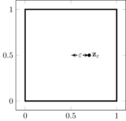
Figure 4: Perturbation $\mathcal{T}_{\varepsilon}$ (blue) of the criss-cross triangulation $\mathcal{T}_{0}$ (gray) of the square

Step 3 (bound of $\mathcal{I}_{1}$): Let $\mathbf{w}_{\mathbf{S}}\in\mathbf{X}_{\eta}(\mathcal{T})$ be arbitrary and recall $\left|K\right|\leq h_{\mathbf{z}}^{2}$ for all $K\in\mathcal{T}_{\mathbf{z}}$ by definition. Since $A_{\mathcal{T},\mathbf{z}}\left(\operatorname*{div}\mathbf{w}_{\mathbf{S}}\right)$ vanishes and $\Theta\left(\mathbf{z}\right)\leq\eta$ for every $\mathbf{z}\in\mathcal{C}_{\mathcal{T}}\left(\eta\right)$ by definition, (38)–(39) and Corollary 1 applied to $\mathbf{v}_{\mathbf{S}}-\mathbf{w}_{\mathbf{S}}\in\mathbf{S}_{k,0}\left(\mathcal{T}\right)$ imply

$$\left\|\operatorname*{div}\mathbf{v}_{\mathbf{S}}\right\|_{L^{2}\left(\Omega\right)} \leq\sqrt{12/7}\zeta_{k-1}^{-1}\sqrt{\sum_{\mathbf{z}\in\mathcal{C}_{\mathcal{T}}\left(\eta\right)}h_{\mathbf{z}}^{2}\left(A_{\mathcal{T},\mathbf{z}}\left(\operatorname*{div}\mathbf{v}_{\mathbf{S}}-\operatorname*{div}\mathbf{w}_{\mathbf{S}}\right)\right)^{2}}$$

$$\leq\sqrt{12/7}\zeta_{k-1}^{-1}k^{2}\sqrt{\sum_{\mathbf{z}\in\mathcal{C}_{\mathcal{T}}\left(\eta\right)}\Theta\left(\mathbf{z}\right)^{2}\left\|\nabla\left(\mathbf{u}_{\mathbf{S}}-\mathbf{w}_{\mathbf{S}}\right)\right\|_{\mathbb{L}^{2}\left(\omega_{\mathbf{z}}\right)}^{2}}$$

$$\leq\frac{C_{\operatorname*{inv}}}{\sin^{2}\phi_{\mathcal{T}}}\sqrt{36/7}\zeta_{k-1}^{-1}k^{2}\eta\left\|\nabla\left(\mathbf{u}_{\mathbf{S}}-\mathbf{w}_{\mathbf{S}}\right)\right\|_{\mathbb{L}^{2}\left(\Omega\right)}$$

with an extra factor $\sqrt{3}$ from the finite overlay of the vertex patches $\omega_{\mathbf{z}}$ in the last step. Since $\mathbf{w}_{\mathbf{S}}\in\mathbf{X}_{\eta}(\mathcal{T})$ was arbitrary, this and $\zeta_{k-1}^{-1}k^{2}\lesssim 1$ conclude the proof. ∎

6 Numerical experiments

In this section we report on numerical experiments of the convergence rates for the pressure-wired Stokes elements and investigate the dependence of $\left\|\operatorname*{div}\mathbf{u}_{\mathbf{S}}\right\|_{L^{2}\left(\Omega\right)}$ on $\eta$ and the number of degrees of freedom.
Analytical solution on the unit square. The difference to the classical Scott-Vogelius element stems from the different treatment of near-singular vertices only. Therefore we focus our benchmark on the criss-cross triangulation $\mathcal{T}_{\varepsilon}$ of the unit square $\Omega:=(0,1)^{2}$ with interior vertex $\mathbf{z}_{\varepsilon}:=(1/2+\varepsilon;1/2)$ perturbed by some $0<\varepsilon<1/2$ shown in Fig. 4. For $\varepsilon\ll 1$, this triangulation locally models a critical mesh configuration with $0<\Theta(\mathbf{z}_{\varepsilon})\ll 1$ where in finite arithmetic the classical Scott-Vogelius FEM becomes unstable. Consider the exact smooth solution

$$\mathbf{u}\left(\mathbf{x}\right)=\begin{pmatrix}\phantom{-}\sin^{2}\left(\pi x_{1}\right)\sin\left(\pi x_{2}\right)\cos\left(\pi x_{2}\right)\\ -\sin^{2}\left(\pi x_{2}\right)\sin\left(\pi x_{1}\right)\cos\left(\pi x_{1}\right)\end{pmatrix}, p\left(\mathbf{x}\right)=10^{6}\operatorname*{e}\nolimits^{-\left(x_{1}-0.3\right)^{-2}-\left(x_{2}-32/500\right)^{-2}}+C,$$

to the Stokes problem with body force $\mathbf{F}\equiv\mathbf{f}:=-\Delta\mathbf{u}+\nabla p\in\mathbf{C}^{\infty}\left(\Omega\right)$. The velocity is pointwise divergence-free as it is the vector curl of $\sin^{2}\left(\pi x_{1}\right)\sin^{2}\left(\pi x_{2}\right)$ and $C$ is chosen such that the pressure $p\in L^{2}_{0}(\Omega)$ has zero integral mean.
Optimal convergence of the $h$-method. This benchmark considers uniform red-refinement of the initial mesh $\mathcal{T}_{\varepsilon}$ that subdivides each element into four congruent children by joining the edge midpoints. This refinement strategy does not introduce new near-singular vertices in the refinement and $\Theta(\mathbf{z}_{\varepsilon})$ remains constant throughout the refinement. We consider $\varepsilon=0.01,0.0001,10^{-6},10^{-8}$ that corresponds to $\Theta(\mathbf{z}_{\varepsilon})\approx 2\varepsilon$.

   

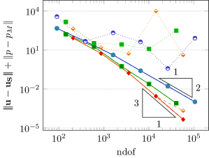
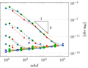
Figure 5: Convergence history of the total error (left) and of the divergence (right) with $\mathbf{z}_{\varepsilon}$ treated as nearly singular $\mathbf{z}_{\varepsilon}\in\mathcal{C}_{\mathcal{T}}(\eta)$ or non-singular $\mathbf{z}_{\varepsilon}\not\in\mathcal{C}_{\mathcal{T}}(\eta)$ vertex for the $h$-method

Fig. 5 displays the total error $\|\nabla(\mathbf{u}-\mathbf{u}_{\mathbf{S}})\|_{\mathbb{L}^{2}(\Omega)}+\|p-p_{M}\|_{L^{2}(\Omega)}$ and the $L^{2}$ norm of the discrete divergence $\|\operatorname*{div}\mathbf{u}_{\mathbf{S}}\|_{L^{2}(\Omega)}$ when $\mathbf{z}_{\varepsilon}\not\in\mathcal{C}_{\mathcal{T}}(\eta)$ is treated as non-singular or as singular $\mathbf{z}_{\varepsilon}\in\mathcal{C}_{\mathcal{T}}(\eta)$ vertex. In the first case, our pressure-wired Stokes FEM is identical to the classical Scott-Vogelius FEM. We observe that for low polynomial degrees $k$ and perturbations $\Theta(\mathbf{z}_{\varepsilon})>10^{-6}$, both variants converge optimally. However, for small perturbations $\Theta(\mathbf{z}_{\varepsilon})<10^{-6}$ (dotted), the solution to the classical Scott-Vogelius FEM is polluted by the high condition number of the algebraic system and only our modification that treats $\mathbf{z}_{\varepsilon}\in\mathcal{C}_{\mathcal{T}}(\eta)$ as nearly singular converges at all and with optimal rate. The divergence of the classical Scott-Vogelius FEM vanishes up to rounding errors except for a similar pollution effect for $\Theta(\mathbf{z}_{\varepsilon})<10^{-6}$. We also observe that the $L^{2}$ norm of the divergence for the pressure-wired Stokes FEM is very small compared to the total error and also significantly smaller than the velocity error $\|\nabla(\mathbf{u}-\mathbf{u}_{\mathbf{S}})\|_{\mathbb{L}^{2}(\Omega)}$ (undisplayed) by a factor of $\Theta(\mathbf{z}_{\varepsilon})$.
Exponential convergence of the $k$-method. This benchmark monitors the behaviour of the $k$-method that successively increases the polynomial degree $k$. The convergence history of the total error in Fig. 6 displays the same pollution effect for small perturbations $0<\varepsilon\ll 1$ or higher polynomial degree $k$ when $\mathbf{z}_{\varepsilon}$ is treated as a non-singular vertex. All other graphs overlay and, in particular, the pressure-wired Stokes FEM converges exponentially. For the discrete divergence, we observe the same convergence up to a certain threshold when accumulated rounding errors dominate. We remark that a sophisticated choice of bases, e.g., from [18], could improve this threshold. However, this does not affect the high condition number caused by the singular mesh configuration that produces the pollution effect for the Scott-Vogelius FEM.

   

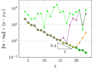
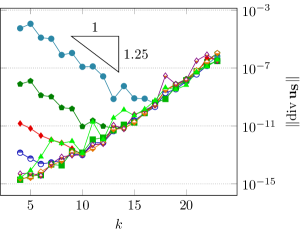
Figure 6: Convergence history of the discretisation error (left) and $\|\operatorname{div}\,\mathbf{u}_{\mathbf{S}}\|$ (right) with $\mathbf{z}_{\varepsilon}$ treated as nearly singular $\mathbf{z}_{\varepsilon}\in\mathcal{C}_{\mathcal{T}}(\eta)$ or non-singular $\mathbf{z}_{\varepsilon}\not\in\mathcal{C}_{\mathcal{T}}(\eta)$ vertex for the $k$-method

References

- \bibcommenthead
- Vogelius [1983] Vogelius, M.: A right-inverse for the divergence operator in spaces of piecewise polynomials. Numerische Mathematik 41(1) (1983)
- Braess [1997] Braess, D.: Finite Elements: Theory, Fast Solvers and Applications in Solid Mechanics. Cambridge University Press, Cambridge (1997)
- Scott and Vogelius [1985] Scott, L.R., Vogelius, M.: Norm estimates for a maximal right inverse of the divergence operator in spaces of piecewise polynomials. RAIRO Modél. Math. Anal. Numér. 19(1) (1985)
- Guzmán and Scott [2019] Guzmán, J., Scott, L.R.: The Scott-Vogelius finite elements revisited. Math. Comp. 88(316) (2019)
- Ainsworth and Parker [2022] Ainsworth, M., Parker, C.: Unlocking the secrets of locking: finite element analysis in planar linear elasticity. Comput. Methods Appl. Mech. Engrg. 395, 115034–56 (2022)
- Bernardi and Raugel [1985] Bernardi, C., Raugel, G.: Analysis of some finite elements for the Stokes problem. Math. Comp. 44(169) (1985)
- Sauter [arXiv:2204.01270, 2022] Sauter, S.A.: The inf-sup constant for Crouzeix-Raviart triangular elements of any polynomial order (arXiv:2204.01270, 2022)
- John et al. [arXiv:2206.01242, 2022] John, V., Li, X., Merdon, C., Rui, H.: Inf-sup stabilized Scott–Vogelius pairs on general simplicial grids by Raviart–Thomas enrichment (arXiv:2206.01242, 2022)
- Arnold et al. [1984] Arnold, D.N., Brezzi, F., Fortin, M.: A stable finite element for the Stokes equations. Calcolo 21(4) (1984)
- Falk and Neilan [2013] Falk, R.S., Neilan, M.: Stokes complexes and the construction of stable finite elements with pointwise mass conservation. SIAM J. Numer. Anal. 51(2) (2013)
- Boffi et al. [2013] Boffi, D., Brezzi, F., Fortin, M.: Mixed Finite Element Methods and Applications. Springer Series in Computational Mathematics, vol. 44. Springer, Heidelberg (2013)
- Ern and Guermond [2021] Ern, A., Guermond, J.-L.: Finite Elements II—Galerkin Approximation, Elliptic and Mixed PDEs. Springer, Cham (2021)
- Brenner [2015] Brenner, S.C.: Forty years of the Crouzeix-Raviart element. Numer. Methods Partial Differential Equations 31(2) (2015)
- Girault and Raviart [1986] Girault, V., Raviart, P.: Finite Element Methods for Navier-Stokes Equations. Springer, Berlin (1986)
- Schwab [1998] Schwab, C.: - and -finite Element Methods. The Clarendon Press Oxford University Press, New York (1998). Theory and applications in solid and fluid mechanics
- Carstensen and Sauter [2022] Carstensen, C., Sauter, S.: Critical functions and inf-sup stability of Crouzeix-Raviart elements. Comput. Math. Appl. 108 (2022)
- Golub and Van Loan [1996] Golub, G.H., Van Loan, C.F.: Matrix Computations, 3rd ed edn. Johns Hopkins studies in the mathematical sciences. Johns Hopkins University Press, Baltimore (1996)
- Beuchler and Schöberl [2006] Beuchler, S., Schöberl, J.: New shape functions for triangular p-FEM using integrated Jacobi polynomials. Numer. Math. 103(3) (2006)