Chemistry Lab Automation via Constrained Task and Motion Planning

Abstract

Chemists need to perform many laborious and time-consuming experiments in the lab to discover and understand the properties of new materials. To support and accelerate this process, we propose a robot framework for manipulation that autonomously performs chemistry experiments. Our framework receives high-level abstract descriptions of chemistry experiments, perceives the lab workspace, and autonomously plans multi-step actions and motions. The robot interacts with a wide range of lab equipment and executes the generated plans. A key component of our method is constrained task and motion planning using PDDLStream solvers. Preventing collisions and spillage is done by introducing a constrained motion planner. Our planning framework can conduct different experiments employing implemented actions and lab tools. We demonstrate the utility of our framework on pouring skills for various materials and two fundamental chemical experiments for materials synthesis: solubility and recrystallization.

I Introduction

Chemistry experiments are essential for finding novel materials or verifying hypotheses in materials science. These experiments are typically conducted by human chemists. They are laborious, time-consuming, and often challenging to reproduce. There is a growing effort to realize self-driving labs [1, 2] reducing the work of chemists and accelerating material discovery. These are automated chemistry labs that close the loop between autonomously (a) selecting the next experiments to run, (b) executing them in the lab using robotic equipment, and (c) evaluating their outcomes, feeding back the results to the experiment selection module.

Challenges and Proposed Solutions. One of the main challenges in realizing the promise of full automation in chemistry labs is the over-reliance on specialized hardware that is tailored to conduct a small part of the overall experiment, and is often immutable and not programmable. This makes adaptation of custom lab equipment to perform multiple types of experiments exceedingly difficult.

Our work aims to address this challenge by enabling general-purpose robot manipulators to autonomously execute chemistry experiments that are described in a high-level abstract specification language. We present a robotic system that incorporates perception, constrained task and motion planning, and vision-based evaluation of experimental outcomes. It satisfies requirements (b) and (c) mentioned above for a number of fundamental chemistry experiments that involve pouring of liquids, solubility, and re-crystallization.

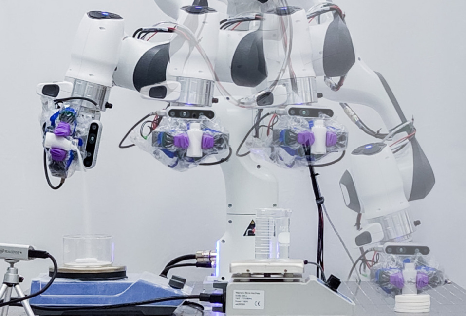
Figure 1: Robot pouring granular material during an experiment.

A second central challenge in chemistry lab automation is ensuring safety during experiment execution and interactions with chemists [3]. Safety requirements can be multi-layered. At a high-level, in terms of experiment description and task planning, we can impose the constraint that materials can be synthesized in a specific order. At a low-level, in terms of manipulation and perception skills, robots should adjust their motion so as to not spill the contents of chemistry vials and beakers during transportation. Our system is able to effectively address both types of safety requirements by expressing them as constraints in terms of task planning as well as motion planning.

Desiderata and Capabilities. There are a number of key enabling capabilities that are needed to robustly address the challenges above. Chemistry robots are required to be equipped with a rich repertoire of general and chemistry domain-specific perception and manipulation skills. They must be able to recognize transparent objects such as glassware, opaque tools, liquids, powders and other substances; segment and recognize the contents of vessels; and estimate object poses [4, 5]. Robots should perceive and monitor the state of the material’s synthesis; for example, they should detect when a solution is fully dissolved [6]. They need to perform dexterous manipulation and handling of objects. Some examples are constrained motion generation for picking and transporting beakers while avoiding spillage of their contents; pouring skills; manipulating tools, rigid objects, and deformable objects. Moreover, robot-executed chemistry experiments require high precision and repeatability to achieve reproducible and reliable results.

Contributions. Our paper presents three major contributions: (I) An autonomous robotic system and modular system for chemistry lab automation that receives as input an abstract experiment description from chemists, perceives the environment, and plans long-horizon trajectories that perform a diverse set of multi-step chemistry experiments. This is an advancement from [7], where a finite state machine with fixed objects in a static workspace was used to perform chemistry experiments. (II) We incorporate constrained motion planning in a PDDLStream [8] solver. This enables long-horizon, multi-task planning and reasoning, while avoiding spillage when transporting liquids and powders. To enhance the success rate of planning in the presence of motion constraints, we have shown that the addition of a degree of freedom to commercial 7-DoF robot arms can be beneficial. We show that the 8-DoF robot has 97% success rate in constrained motion planning compared to 84% of the 7-DoF robot. (III) We present and analyze a set of accurate and efficient pouring skills inspired by human motions. It has an average relative error of 8.1% and 8.8% for pouring water (liquid) and salt (granular solids) compared to a baseline method with 81.4% and 24.1% errors. These results are comparable with recent results [9, 10], while our method is simpler, and require fewer and simpler sensors.

As a proof of concept, we have shown that by closing the loop with the perception of the current status of the chemistry experiment under execution, we can achieve results comparable to the literature ground truth for solubility experiment. We attained 7.2 % error for the solubility of salt and successfully recrystallized alum.

II Related Work

Lab Automation

Lab automation aims to introduce automated hardware in a laboratory to improve the efficiency of scientific findings. An example of lab automation is the usage of mobile robots for improving photocatalysts for hydrogen production from water [11]. Recently, an automated workflow that translates organic chemistry literature into a structured language called XDL was proposed [12]. ARChemist [7], a lab automation system, was developed to conduct experiments including solubility screening and crystallization without human intervention. Although these major steps towards chemistry lab automation have been made, their dependence on predefined tasks and motion plans without constraint satisfaction guarantees limits their flexibility in new and dynamic workspaces. In those works, pick & place was the primary task that the manipulators were carrying out. Those works were tested in hand-tuned and static environments to avoid occurrences of unsatisfied task constraints, such as chemical spills from vessels filled with liquid during transfer. Our framework resolves these gaps through constraint satisfaction and scene-aware planning with a variety of skills.

Task and Motion Planning with Constraints

Task and motion planning (TAMP) simultaneously determines the sequence of high-level symbolic actions, such as picking and placing, and low-level motions for the action, such as trajectory generation. Another TAMP solver, PDDLStream [8], extends PDDL [13], a common language to describe a planning problem mainly targeting discrete actions and states, by introducing streams, a declarative procedure via sampling procedures. PDDLStream reduces a continuous problem to a finite PDDL problem and invokes a classical PDDL solver as a subroutine. Since PDDLStream verifies the feasibility of action execution during planning time, it can inherently enhance safety by avoiding unfeasible plans or plans that may lead to unsafe situations. Nonetheless, PDDLStream does not yet account for constraints in the planning process, for example avoiding material spillage from beakers during transportation, which impedes its deployment in real-world lab environments. For this purpose, sampling-based motion constraint adherence [14] or model-based motion planning [15] are possible stream choices. To overcome this shortcoming, our work extends PDDLStream with a projection-based sampling technique [16] to provide constraint satisfaction, completeness, and global optimality.

Skills and Integration of Chemistry Lab Tools

In the process of lab automation, robots interact with tools and objects within the workspace and require a repertoire of many laboratory skills. Some skills can be completed with existing heterogeneous instruments and sensors in chemistry labs, such as scales, stir plates, pH sensors, and heating instruments. Other skills are currently done either manually by humans in the lab or with expensive special instruments. In a self-driving lab, robots should acquire those skills by effectively using different sensory inputs to compute appropriate robot commands. Pouring is a common skill in chemistry labs. Recent work [9, 10] used vision and weight feedback to pour liquid with manipulators. [9] proposed optimal trajectory generation combined with system identification and model priors. To achieve milliliter accuracy in water pouring tasks with a variety of vessels at human-like speeds, [10] used self-supervised learning from human demonstrations. In this work, we have reached similar results for pouring, using commercial scales that have delayed feedback. Our approach is model-free, and it can pour granular solids as well. Granular solids have different dynamics from liquids, similar to the avalanche phenomenon. Lastly, while executing a chemistry experiment, the robot should possess perception skills to measure progress toward completing the task. For example, in solubility experiments, the robot should perceive when the solution is fully dissolved, and therefore stop pouring the solvent into the solution. There are different ways to measure solubility. In our work, we use the turbidity measure [6], which is based on optical properties of light scattering and absorption by suspended sediment [17].

III Methods

Figure 2: Framework for robot-assisted chemical synthesis: composed of Perception, Task & Motion Planning, and Skills blocks. Our framework enables the robot to leverage available chemistry lab devices (including sensors and actuators) by adding them to the robot network through ROS. The robot is equipped with an additional DOF at the end-effector, allowing it to perform constrained motions. Our framework receives the chemical synthesis goal in XDL format. The procedure component is converted into corresponding PDDL goals, and hardware and reagents components identify the required initial condition for synthesis. Perception detects objects and estimates their positions, contents in the workspace, and task progress. PDDLStream generates a sequence of actions for the robot execution.

Framework Overview

Our proposed framework consists of three components: perception, task and motion planning (TAMP), and a set of manipulation skills, as shown in Fig. 2. The Chemical Description Language (XDL) [12] provides a high-level description of experiment instructions as an input to the TAMP solver. The perception module updates the scene description by detecting the objects and estimating their positions using fiducial markers [18]. Currently, we assume prior knowledge of vessel contents and sizes, and each vessel is mapped to a unique marker ID. Given the instructions from XDL and the instantiated workspace state information from perception, a sequence of high-level actions and a robot trajectory are simultaneously generated by the PDDLStream TAMP solver. The resulting plan is then realized by the manipulation module and robot controller, while closing the loop with perception feedback, such as updated object positions and status of the solution.

III-A Task and Motion Planning for Chemistry Experiments

The TAMP module converts experiment instructions given by XDL into PDDLStream goals and generates a motion plan. The TAMP algorithm is shown in Alg. 1.

PDDLStream

A PDDLStream problem described by a tuple $(\mathcal{P},\mathcal{A},\mathcal{S},\mathcal{O},\mathcal{I},\mathcal{G})$ is defined by a set of predicates $\mathcal{P}$, actions $\mathcal{A}$, streams $\mathcal{S}$, initial objects $\mathcal{O}$, an initial state $\mathcal{I}$, and a goal state $\mathcal{G}$. A predicate is a boolean function that describes the logical relationship of objects. A logical action $a\in\mathcal{A}$ has a set of preconditions and effects. The action $a$ can be executed when all the preconditions are satisfied. After execution, the current state changes according to the effects. The set of streams, $\mathcal{S}$, distinguishes a PDDLStream problem from traditional PDDL. Streams are conditional samplers that yield objects that satisfy specific constraints. The goal of PDDLStream planning is to find a sequence of logical actions and a continuous motion trajectory starting from the initial state until all goals are satisfied, ensuring that the returned plan is valid and executable by the robot. We define four types of actions in our PDDLStream domain, including pick, move, place, and pour. For example, the move action translates the robot end-effector from a grasping pose to a placing or pouring pose using constrained motion planning. PDDLStream handles continuous motion using streams. Streams generate objects from continuous variables that satisfy specified conditions, such as feasible grasping pose and collision-free motion. An instance of a stream has a set of certified predicates that expands $\mathcal{I}$ and functions as preconditions for other actions.

A PDDLStream problem is solved by invoking a classical PDDL planner [19] with optimistic instantiation of streams (Alg. 1, line 7). If a plan for the PDDL problem is found, the optimistic stream instances $s\in\mathcal{S}$ in the plan are evaluated to determine the actual feasibility (Alg. 1, line 8). If no plan was found or the streams are not feasible, other plans are explored with a larger set of optimistic stream instances.

Chemical Description Language (XDL)

XDL [12] is a chemical description language that describes chemical experiments in a standard XML format. It is based on XML syntax and is mainly composed of three mandatory sections: Hardware, Reagents, and Procedure. We parse XDL instructions and pass them to the TAMP module. The Hardware and Reagents sections are parsed as initial objects $\mathcal{O}$. Procedure is translated into a set of goals $Goals$ (line 1). $\mathcal{I}$ is generated from $\mathcal{O}$ and sensory inputs (line 2). Each intermediate goal $\mathcal{G}\in Goals$ is processed by PDDLStream (line 5). If a plan to attain $\mathcal{G}$ is found, it is stored (line 10) and $\mathcal{I}$ is updated according to the plan (line 11). After a set of plans to attain all goals is found, we obtain a complete motion plan (line 12).

Task and Motion Plan Refinement at Execution Time

We adopt two considerations for the dynamic nature of chemistry experiments: motion plan refinement and task plan refinement.

The generated motion plan is refined to reflect the updated status of the scene and to overcome the perception errors. The initial object pose detection may contain errors, therefore, the object may not be placed in the expected position during execution. This error arises from two reasons. First, when the robot interacts with the objects in the workspace, their position changes, for example when regrasping an object after placing it in the workspace. This change is not foreseeable by the planner ahead of time. Therefore, to improve the success rate, the object pose is estimated just before grasping, and the trajectory is refined. We assume that the perturbation of the perceived state of the objects is bounded so that it does not cause a change in the logical state of the system, which would necessitate task-level replanning.

In addition to motion refinement, we consider task plan refinement. Task execution is repeated using the feedback from perception modules at execution time to support conditional operations in chemistry experiments, such as adding acid until pH reaches 7. The number of repetitions required to satisfy conditions is unknown at planning time, so the task plan is refined at execution time.

1:A XDL recipe $\mathcal{\chi}$, sensory input $\mathcal{H}$, PDDLStream domain $\mathcal{D}$

2:Reference $plan$ to execute

3:$Goals,\mathcal{O}\leftarrow$xdlParser($\mathcal{\chi}$) $\triangleright$ Objects

4:$\mathcal{I}\leftarrow$ perception($\mathcal{H},\mathcal{O}$) $\triangleright$ Initial conditions

5:if not passConditions($\mathcal{I}$, $\mathcal{O}$) then return

6:$plan=\emptyset$, $\mathcal{P}=\emptyset$

7:for all $\mathcal{G}\in Goals$ do

8:    while $time()\leq t_{max}$ do

9:       $\mathcal{P}$ = optimisticPddlStreamPlan($\mathcal{I}$, $\mathcal{G}$, $\mathcal{D}$)

10:       if $\mathcal{P}\neq\emptyset$ and isStreamFeasible($\mathcal{P}$) then break     

11:    if $\mathcal{P}=\emptyset$ then return

12:    $plan\leftarrow plan\cup\mathcal{P}$

13:    $\mathcal{I}$ = updateSceneRepresentation($\mathcal{I},\mathcal{P}$)

14:return $plan$

Algorithm 1 TampForLabAutomation()

III-B Motion Constraints for Spillage Prevention

Unlike pick-and-place of solid objects, robots in a chemistry lab need to carry beakers that contain liquids, powders, or granular materials. These chemicals are sometimes harmful, so the robot motion planner should incorporate constraints to prevent spillage. To this end, an important requirement for robot motion is the orientation constraints of the end-effector. To avoid spillage, the end-effector orientation should be kept in a limited range while beakers are grasped. We incorporated constrained motion planning in the framework to meet these safety requirements, under the assumption of velocity and acceleration upper bounds. Moreover, we introduced an additional (8th) degree of freedom to the robot arm, in order to increase the success rate of constrained motion planning. We empirically observed no spillage as long as orientation constraints are satisfied in the regular acceleration and velocity of the robot end-effector, particularly since beakers are not filled to their full capacity in a chemistry lab.

1:for all  $i\in trials$ do

2:    $\bm{q}_{g}\leftarrow$ solveIK($(^{\mathcal{I}}\bm{p}_{\mathcal{B}},^{\mathcal{I}}{\bm{R}}_{\mathcal{B}})$)

3:    pathPlanner$\leftarrow$ init($\bm{q}_{0},\bm{q}_{g}$)

4:    while  $path~{}\text{is}~{}\emptyset$ do

5:       $\bm{q}\leftarrow$ sample()

6:       while $\|\bm{\mathcal{F}}(\bm{q})\|>\epsilon$ do

7:          $\delta\bm{q}\leftarrow\bm{\mathcal{J}}^{\dagger}(\bm{q})\bm{\mathcal{F}}(\bm{q})$

8:          $\bm{q}\leftarrow\bm{q}-\delta\bm{q}$        

9:       $path\leftarrow$ pathPlanner($\bm{q})$     

10:    if $path\neq\emptyset$ then return $path$

11:return $path$

Algorithm 2 ConstrainedMotionPlanning()

Constrained motion planning: First, an IK solver is executed with multiple random initializations  [20]. Then, PRM^⋆ is initialized [21]. PRM^⋆ graph grows using projected samples that satisfy the constraints (red). This process iterates until a motion plan is found.

Constrained Motion Planning

Given a robot with $n$ degrees of freedom in the workspace $\mathcal{Q}\in\mathbb{R}^{n}$ with obstacle regions $\mathcal{Q}_{obs}\in\mathbb{R}^{n}$, the constrained planning problem can be described by finding a path in the manipulator’s free configuration space $\mathcal{Q}_{free}=\mathcal{Q}-\mathcal{Q}_{obs}$ that satisfies initial configuration $\bm{q}_{0}\in\mathbb{R}^{n}$, end-effector goal pose $(^{\mathcal{I}}\bm{p}_{\mathcal{B}}\in\mathbb{R}^{3},^{\mathcal{I}}{\bm{R}}_{\mathcal{B}}\in SO(3))$, and equality path constraints $\bm{\mathcal{F}}(\bm{q}):\mathcal{Q}\to\mathbb{R}^{k}$. The constrained configuration space can be represented by the implicit manifold $\mathcal{M}=\{q\in\mathcal{Q}\ |\ \bm{\mathcal{F}}(\bm{q})=\textbf{0}\}$. The implicit nature of the manifold prevents planners from directly sampling, since the distribution of valid states is unknown. Further, since the constraint manifold resides in a lower dimension than the configuration space, sampling valid states in the configuration space is highly improbable and thus impractical. Following the constrained motion planning framework developed in [16, 22], our framework integrates the projection-based method for finding constraint-satisfying configurations during sampling as described in Alg. 2. In this work, the constraints are set to the robot end-effector, hence they can be described with geometric forward kinematics, with its Jacobian defined as $\bm{\mathcal{J}}(\bm{q})=\frac{\delta\bm{\mathcal{F}}}{\delta\bm{q}}$. After sampling from $\mathcal{Q}_{free}$ in line 5, projected configurations $\bm{q}$ are found by minimizing $\bm{\mathcal{F}(q)}$ iteratively using Newton’s method (highlighted in red). We use probabilistic roadmap methods (PRM^⋆) to plan efficiently in the 8-DoF configuration space found in our chemistry laboratory domain [21, 23].

The constrained path planning problem is sensitive to the start and end states of the requested path, since paths between joint states may not be possible under strict or multiple constraints. If constrained planning is executed with any arbitrary valid solution from the IK solver, the planner typically fails. To address this shortcoming, three considerations are made. First, a multi-threaded IK solver with both iterative and random-based techniques is executed, and the solution that minimizes an objective function $\phi$ is returned [20]. During grasping and placing, precision is paramount, and we only seek to minimize the sum-of-squares error between the start and goal Cartesian poses. Second, depending on the robot task, the objective function is extended to maximize the manipulability ellipsoid as described in [24], which is applied for more complicated maneuvers, such as transferring liquids across the workspace. Finally, note that configuration sampling must account for the fact that multiple goal configurations are possible. For this purpose, Alg. 2 can iterate several times to find various goal configurations in line 2.

An 8-DoF Robot Arm

To increase the success rate of planning and grasping under non-spillage constraints, we introduced an additional degree of freedom to the 7 DoF Franka robot. The aim of the addition is twofold. First, the 8-DoF robot has a higher empirical success rate in constrained motion planning, which leads to a higher success rate in total task and motion planning. Second, the robot end-effector orientation is changed to flat (parallel to the floor). This usually places the end-effector orientation far from the joint limit, which in turn makes the pouring control easier.

III-C Manipulation and Perception Skills

Chemistry lab skills require a particular suite of sensors, algorithms, and hardware. We provide an interface for instantiating different skill instances through ROS and simultaneously commanding them. For instance, recrystallization experiments in chemistry require both pouring, heating, and stirring, which uses both weight feedback for volume estimation and skills for interacting with the liquid using available hardware.

Pouring Controller

In chemistry labs, a frequently used skill in chemical experiments is pouring. Pouring involves high intra-class variations depending on the underlying objective (e.g. reaching a desired weight or pH value); the substances and material types being handled (e.g. granular solids or liquids); the glassware being used (e.g., beakers and vials); the overall required precision; and the availability of accurate and fast feedback. Pouring is a closed-loop process, in which feedback should be continuously monitored. Among these pouring actions, in our work we consider the following variations: pouring of liquids and granular solids. Note that, in contrast to many control problems, pouring is a non-reversible process as we cannot compensate for overshoot (as the poured material cannot go back to the pouring beaker).

Inspired by observations of chemists pouring reagents, we propose a controller that allows the robot to perform different pouring actions. As shown in Fig. 3, the proposed method takes sensor measurements (e.g. weight feedback from the scale) as feedback and a reference pouring target. The algorithm outputs the robot end-effector joint velocity describing oscillations of the arm’s wrist. Since sensors are characterized by measurement delays, chemical reactions require time to stabilize, and pouring is a non-reversible action, chemists tend to conservatively pour a small amount of content from the pouring vessel into the target vessel. They periodically wait for some time to observe any effects and then pour micro-amounts again. In our approach, we use a shaping function $s(t)$ to guide the direction and frequency of this oscillatory pouring behavior, while a PD controller lowers the pouring error. The end-effector velocity vector is computed by convolving the shaping function $s(t)$ over the PD control signal, $\bm{v}_{\mathrm{PD}}(t)=\bm{k}_{p}e+\bm{k}_{d}\dot{e}$, where $e(t)=x_{ref}-x_{fb}$. Fig. 4 shows an example of the angular velocity of the end-effector and the error during actual pouring.

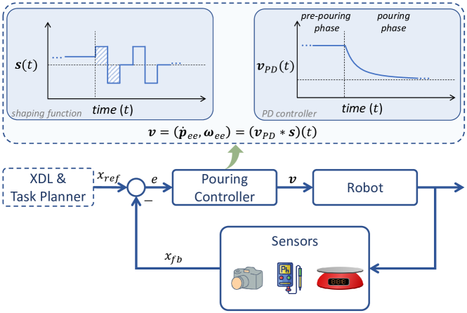
Figure 3: Pouring skill controller: given the XDL & TAMP reference values and sensor feedback, the pouring controller computes the end-effector velocity for the robot using the convolution of a shaping function $\bm{s}(t)$ and a PD control output $\bm{v}_{PD}(t)$.

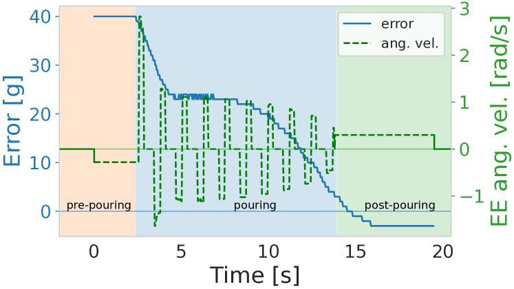
Figure 4: An example of pouring control. The velocity of the end-effector is controlled based on the feedback error and shaping function.

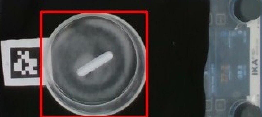
Figure 5: An example of automated turbidity measurement. The camera detects the Petri dish using Hough Circle Transform. The average brightness of the detected area (red square) is used as a proxy of turbidity.

Turbidity-based Solubility Measurement

Solubility of a solute is measured by determining the minimum amount of solvent (water) required to dissolve all solutes at a given temperature when the overall system is in equilibrium [6]. Since the solutions get transparent when all solutes dissolve into water, turbidity, or opaqueness of the solution, is used as the metric to determine the completion of the experiment. The average brightness of the solution was used as a proxy for the relative turbidity, inspired by HeinSight [6]. It compared the current measured turbidity value with reference value (coming from pure solvent) to determine when the solution is dissolved. Differently from them, we use the relative turbidity changes using the current and previous measurement values to detect when the solution is dissolved. Moreover, to make the perception pipeline autonomous, when the robot with an in-hand camera observes the dish containing the solution, it detects the largest circular shape as the dish using Hough Circle Transform implemented in OpenCV. The square region containing the dish is converted into HSV color space, and the average Value (brightness) of the region is used as a turbidity value. Figure 5 shows an example of the automated turbidity measurement. Although the detected area contains the dish and stir bar, they do not affect the relative value because these are a constant bias in all measurements.

IV Experiments and Evaluation

We evaluate the proposed framework with two component studies on pouring and constrained TAMP, and two types of experiments, solubility and recrystallization.

IV-A Experiment Setup

Hardware

The proposed lab automation framework has been evaluated using the Franka Emika Panda arm robot, equipped with a Robotiq 2F-85 gripper and an Intel RealSense D435i stereo camera mounted on the gripper to allow for active vision. The robot’s DoF has been extended by one degree (in total 8 DoF) at its end-effector using a Dynamixel XM540-W150 servo motor. Fig. 2 shows the hardware setup.

Lab Tools Integration

The robot framework is expanded by incorporating lab tools. We used an IKA RET control-visc device, which works as a scale, hotplate, and stir plate, and Sartorius BCA2202-1S Entris, which works as a high-precision weighing scale. The devices communicate with the TAMP solver to execute chemistry specific skills.

Software

The robot is controlled using FrankaPy [25]. We implemented a ROS wrapper for the servo motor (8th DoF). To detect fiducial markers, we use the AprilTag library [18]. We use the MoveIt motion planning framework [26] for our TAMP solver and its streams. The constrained planning function [16] is an extension of elion [27].

Chemistry Experiments

We evaluated our framework by conducting solubility measurement experiments as well as recrystallization experiments. Solubility is a basic property of the solute and solvent, and measuring it is a well-known basic experiment in chemistry [28]. Measuring solubility has desirable characteristics as a benchmark for automated chemistry experiments: (i) it requires basic chemistry operations, such as pouring, solid dispensing, and observation of the solution status, (ii) solubility can be measured using ubiquitous food-safe materials, such as water, salt, sugar, and (iii) the accuracy of the measurement can be evaluated quantitatively by comparing with literature values. We also conducted a recrystallization experiment to show the flexibility of our framework and its ability to handle a diverse set of experiments. We attained $7.2\%$ error for salt solubility and successfully recrystallized alum.

IV-B Safety Evaluation of Motions Without Spillage

Constrained Motion Planning in 7/8 DoF robot

The constrained motion planning performance of 7 DoF and 8 DoF robot is evaluated in two scenarios: (1) single step, (2) two steps. In scenario (1), robots find a constrained path with a fixed orientation from initial to final positions that are randomly sampled. Scenario (2) extends the first with an additional intermediate sampled waypoint. For each scenario, we run 50 trials in Alg. 2 with random seeding of the IK solver. In scenario (2), we restart the sequence planning from the first step if a step fails. Constraints are set to the robot end-effector pitch and roll ($\|\theta,\phi\|\leq 0.1\text{ rad}$).

The performance of the 7-DoF and 8-DoF robot arms for the two scenarios are shown in Table I. The results show that the IK and constrained motion planning have higher success rates in 8-DoF compared with the 7-DoF robot.

TABLE I: Success rate comparison of 7 and 8-DoF robot.

	Scenario 1 (%)		Scenario 2 (%)
	IK	Plan	IK	Plan
7 DoF	99	84	99	70
8 DoF	100	97	100	84

IV-C Pouring Skill Evaluation

We evaluated accuracy and efficiency of pouring skill of liquid and powder. To evaluate the effect of our proposed pouring method, we implemented a PD control pouring method where end-effector angular velocity is proportional to the difference between target and feedback weight as a baseline. Fig. 6 shows the pouring experiment results. The results show that the shaping function contributed to reducing the overshooting compared to PD control pouring. The overshoot of the PD control pouring is mainly because of the scale’s delayed feedback ($\sim$3 s). The intermittent pouring caused by the shaping function compensated for the delay and improved the overall pouring accuracy. On average the pouring error using shaping approach is $2.2\pm 1.5$ g and for PD control is $24.5\pm 12.0$ g and their average relative error and standard deviation are $8.1\pm 4.8$ % and $81.4\pm 4.5$ %. Moreover, as we can see both the error and relative errors stays constant when using shaping method in contrast to the PD controller. The average pouring time with shaping function of 50 mL water and salt were 25.1 s and 36.8 s. Our results are comparable with previous work [9, 10] in terms of pouring error and time, without using a learned, vision-based, policy, or expensive equipment setup.

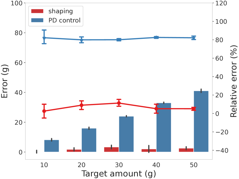
(a) Pouring error in water.

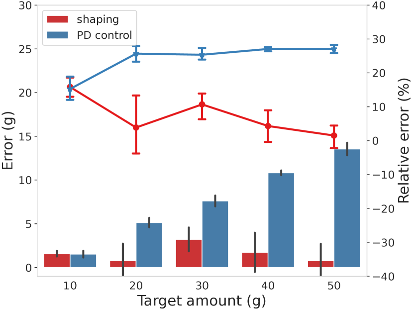
(b) Pouring error in salt.

Figure 6: Evaluation of pouring error. The pouring errors of our shaping pouring and PD control baseline pouring are compared using (a) water and (b) salt. The bar plot shows the error (poured amount - target amount) and the line plot shows the relative error. The error bars show the standard deviation.

IV-D Solubility Experiments

We measured the solubility of three solutes, table salt (sodium chloride), sugar (sucrose), and alum (aluminum potassium sulfate). The workflow of the solubility experiments is shown in Fig. 7. The robot continues pouring water until turbidity stops changing. The measured solubility for three solutes is shown in Table II. The robot framework managed to measure the solubility with accuracy that is comparable to solubility values found in the literature [29].

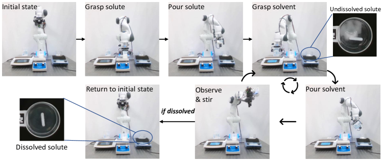
Figure 7: Workflow of solubility experiment. First, a fixed amount of the solute is added to the dish on the weighing scale and stirrer. The robot pours 10 g of water into the dish. The solution is mixed with the magnetic stirrer. After stirring, the turbidity of the solution is measured to check dissolvement. If undissolved, another 10 g of water is added until no solutes remain. The experiment was conducted at room temperature (25^∘C).

TABLE II: Results of the solubility experiments. Amount of solute in the beaker, amount of water to dissolve all solute, calculated solubility (the amount of solute dissolved per 100 g of water), and literature data for solubility at 20^∘C is shown. Literature data are taken or calculated from [29].

solute	solute [g]	water [g]	solubility	lit. data	% error
Salt	13.9	41.8	33.2	35.8	7.2
Sugar	60.00	26.46	226.8	203.9	11.2
Alum	3.00	29.87	10.0	11.4	12.3

The primary reason for the difference from the literature value is the range of minimum amount of water required for dissolving. In an example of turbidity change shown in Fig. 8, the robot can only tell the second pouring is insufficient and the third pouring is sufficient to dissolve all solutes, but it cannot tell the exact required amount. As a result, the solubility measurement inherently includes error caused by the resolution of pouring. We can reduce the error by pouring a smaller amount of water at once, but pouring smaller than 10 g is difficult because of the delayed feedback of the scale and the scale minimum resolution. We can improve the accuracy of solubility measurement by developing a pipette designed for a robot.

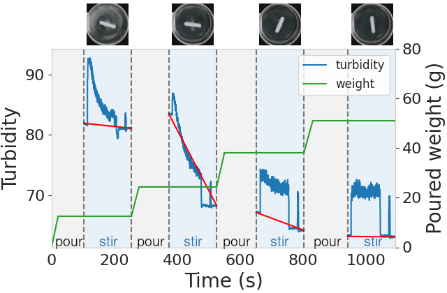
Figure 8: Turbidity change during experiment. Water is poured into the dish during pouring (grey) and turbidity is measured during observation (blue). The end of the experiment is determined by turbidity comparison. In this example, all solutes are dissolved at the third pouring because the turbidity change after the fourth pouring is below the threshold. The average weight of the second and third pouring is used to calculate the solubility.

We evaluated the success rate of the solubility experiment by conducting several trials. An experiment is considered successful when the robot could execute all actions without aborting and could calculate solubility. Without execution time refinement, 5 out of 9 experiments were successful, i.e., $\sim 56\%$ success rate. Further results are available on the website. Note that human errors, such as incorrect software handling, were excluded from the calculation. Two types of failures were observed; i) TAMP failure: a plan was not found because of infeasible inverse kinematics or motion planning request; ii) inconsistency between planning and actual environment: perception error and simplification of object shape in planner caused inconsistency of two environments and collisions occurred at execution time.

IV-E Recrystallization Experiments

Recrystallization is a purifying technique to obtain crystals of a solute by using the difference in solubility at different temperatures. Typically, solutes have higher solubility at high temperatures, meaning hot solvents will dissolve more solute than cool solvents. The excess amount of solute that cannot be dissolved anymore while cooling the solvent precipitates and forms crystals. We tested the recrystallization of alum by changing the temperature of the water. Alum was chosen as the target solute since its solubility greatly changes according to water temperature. The recrystallization experiment setup extends the solubility test by pre-heating the solvent. Fig. 9 show the result of the experiment.

Figure 9: Recrystallization of alum inside the water. After heating water by putting a beaker with water on a hotplate, the robot poured alum into a dish. The robot then poured hot water, and the solution was heated and stirred. The formation of a precipitate is observed after the dish is cooled down. The dried crystals in a vial are shown.

IV-F Discussion and Limitations

Our results show the proposed TAMP pipeline can effectively perform multi-step chemistry experiments from an experiment description in XDL. However, the current study is limited to two types of chemistry experiments because the number of skills incorporated in the framework is limited. Increasing the repertoire of skills, such as glassware perception in 3D and clutter, without fiducial markers [30], can improve the framework scalability. Also, PDDLStream inefficiency inhibits the framework from being reactive in a dynamic environment. Incorporating the learning-based search heuristics for PDDLStream [31] may overcome this limitation. Constrained motion planning was shown to effectively avoid spillage of the beaker contents during transfer in our experiments. We have also shown that adding an extra 8th DoF to the robot enabled more flexibility and a higher success rate for constrained motion planning. However, the proposed constrained motion planning embedded in TAMP cannot run in real-time. Considering the dynamics of the beaker content may help to have higher flexibility in robot manipulation [15]. Although our skill currently has attained 8% error for liquid and powder pouring, higher accuracy is desirable for precise experiments. We used a scale with integrated functionality for stirring and heating, but its measurement is delayed for 3 s. Higher precision pouring can be attained using a scale with a shorter response time; also, it can be achieved by specialized tools, such as a pipette. In addition, visual feedback during pouring may avoid spillage.

V Conclusion

In this paper, we introduced a chemistry lab automation framework using general-purpose robot manipulators that execute long-horizon chemistry experiments in a closed-loop fashion, being able to visually inspect the completion of the experiment. The approach adapts to different chemistry experiments by transforming high-level experiment descriptions written in XDL into a sequence of subgoals planned by TAMP solver. We incorporated perception, constrained TAMP, an 8-DoF robot, and interaction with heterogeneous lab tools and equipment interfaces into our framework. We demonstrated the capabilities of our system by performing different pouring skills, which enabled the robot to handle solubility and recrystallization experiments. We aim to accelerate materials discovery by extending this framework to perform more reliable and effective experiments by learning various skills using simulation tools. We would like to enhance the chemists’ experience by introducing a natural language interface.

References

- [1] M. Seifrid, et al., “Autonomous chemical experiments: Challenges and perspectives on establishing a self-driving lab,” Acc. Chem. Res., vol. 55, no. 17, pp. 2454–2466, 2022.
- [2] M. Abolhasani and E. Kumacheva, “The rise of self-driving labs in chemical and materials sciences,” Nat. Synth., pp. 1–10, 2023.
- [3] A. D. Ménard and J. F. Trant, “A review and critique of academic lab safety research,” Nature chemistry, vol. 12, no. 1, pp. 17–25, 2020.
- [4] H. Xu, et al., “Seeing glass: Joint point-cloud and depth completion for transparent objects,” in Ann. Conf. on Robot Learning, 2021.
- [5] Y. R. Wang, et al., “Mvtrans: Multi-view perception of transparent objects,” arXiv:2302.11683, 2023.
- [6] P. Shiri, et al., “Automated solubility screening platform using computer vision,” Iscience, vol. 24, no. 3, p. 102176, 2021.
- [7] H. Fakhruldeen, et al., “ARChemist: Autonomous robotic chemistry system architecture,” arXiv:2204.13571, 2022.
- [8] C. R. Garrett, et al., “PDDLStream: Integrating symbolic planners and blackbox samplers via optimistic adaptive planning,” in Proceedings of the 30th Int. Conf. on Automated Planning and Scheduling (ICAPS). AAAI Press, 2020, pp. 440–448.
- [9] M. Kennedy, et al., “Autonomous precision pouring from unknown containers,” IEEE Robo. and Automation Letters, vol. 4, no. 3, p. 2317–2324, Jul 2019.
- [10] Y. Huang, et al., “Robot gaining accurate pouring skills through self-supervised learning and generalization,” Robo. and Autonomous Systems, vol. 136, p. 103692, Feb 2021.
- [11] B. Burger, et al., “A mobile robotic chemist,” Nature, vol. 583, no. 7815, pp. 237–241, 2020.
- [12] S. H. M. Mehr, et al., “A universal system for digitization and automatic execution of the chemical synthesis literature,” Science, vol. 370, no. 6512, pp. 101–108, 2020.
- [13] C. Aeronautiques, et al., “PDDL - the planning domain definition language,” Tech. Rep., 1998.
- [14] D. Berenson, et al., “Task space regions: A framework for pose-constrained manipulation planning,” Int. J. Robot. Res., vol. 30, no. 12, pp. 1435–1460, 2011.
- [15] R. I. C. Muchacho, et al., “A solution to slosh-free robot trajectory optimization,” in 2022 IEEE/RSJ Int. Conf. on Intelligent Robots and Systems (IROS). IEEE, 2022, pp. 223–230.
- [16] Z. Kingston, et al., “Exploring implicit spaces for constrained sampling-based planning,” Int. J. Robot. Res., vol. 38, no. 10-11, pp. 1151–1178, 2019.
- [17] B. G. Kitchener, et al., “A review of the principles of turbidity measurement,” Progress in Physical Geography, vol. 41, no. 5, pp. 620–642, 2017.
- [18] E. Olson, “Apriltag: A robust and flexible visual fiducial system,” in 2011 IEEE Int. Conf. on Robo. and automation, 2011.
- [19] M. Helmert, “The fast downward planning system,” J. Artif. Intell. Res., vol. 26, pp. 191–246, 2006.
- [20] P. Beeson and B. Ames, “TRAC-IK: An open-source library for improved solving of generic inverse kinematics,” in 2015 IEEE-RAS 15th Int. Conf. on Humanoid Robots (Humanoids), Nov 2015.
- [21] S. Karaman and E. Frazzoli, “Sampling-based algorithms for optimal motion planning,” Int. J. Robot. Res., vol. 30, no. 7, pp. 846–894, 2011.
- [22] Z. Kingston, et al., “Sampling-based methods for motion planning with constraints,” Annu. Rev. Control Robot. Auton. Syst., vol. 1, pp. 159–185, 2018.
- [23] L. E. Kavraki, et al., “Probabilistic roadmaps for path planning in high-dimensional configuration spaces,” IEEE Trans Rob Autom., vol. 12, no. 4, pp. 566–580, 1996.
- [24] T. Yoshikawa, “Manipulability of robotic mechanisms,” Int. J. Robot. Res., vol. 4, no. 2, pp. 3–9, 1985.
- [25] K. Zhang, et al., “A modular robotic arm control stack for research: Franka-Interface and FrankaPy,” arXiv:2011.02398, 2020.
- [26] D. Coleman, et al., “Reducing the barrier to entry of complex robotic software: a MoveIt! case study,” arXiv:1404.3785, 2014.
- [27] “elion: Constrained planning in MoveIt using OMPL’s constrained planning interface,” https://github.com/JeroenDM/elion, 2020.
- [28] E. Wolthuis, et al., “Determination of solubility: a laboratory experiment,” J. of Chemical Education, vol. 37, no. 3, p. 137, 1960.
- [29] N. A. O. of Japan, Handbook of Scientific Tables. WORLD SCIENTIFIC, 2022.
- [30] S. Eppel, et al., “Computer vision for recognition of materials and vessels in chemistry lab settings and the vector-labpics data set,” ACS central science, vol. 6, no. 10, pp. 1743–1752, 2020.
- [31] M. Khodeir, et al., “Learning to search in task and motion planning with streams,” arXiv:2111.13144, 2021.