Nonequilibrium dynamics of the Ising model on heterogeneous networks with an arbitrary distribution of threshold noise

Abstract

The Ising model on networks plays a fundamental role as a testing ground for understanding cooperative phenomena in complex systems. Here we solve the synchronous dynamics of the Ising model on random graphs with an arbitrary degree distribution in the high-connectivity limit. Depending on the distribution of the threshold noise that governs the microscopic dynamics, the model evolves to nonequilibrium stationary states. We obtain an exact dynamical equation for the distribution of local magnetizations, from which we find the critical line that separates the paramagnetic from the ferromagnetic phase. For random graphs with a negative binomial degree distribution, we demonstrate that the stationary critical behavior as well as the long-time critical dynamics of the first two moments of the local magnetizations depend on the distribution of the threshold noise. In particular, for an algebraic threshold noise, these critical properties are determined by the power-law tails of the distribution of thresholds. We further show that the relaxation time of the average magnetization inside each phase exhibits the standard mean-field critical scaling. The values of all critical exponents considered here are independent of the variance of the negative binomial degree distribution. Our work highlights the importance of certain details of the microscopic dynamics for the critical behavior of nonequilibrium spin systems.

I Introduction

Understanding cooperative phenomena in large interacting complex systems is at the forefront of various branches of science [1, 2, 3, 4]. The Ising model on random graphs provides a general framework to tackle this problem and to explore how heterogeneous interactions among the spins influence their dynamical behavior. Heterogeneity here refers to local fluctuations in the graph topology, such as the number of neighbors coupled to each spin (the so-called degrees [5]).

Universal scaling around phase transitions is perhaps the most striking collective property of spin models [6]. Renormalization group theory and the computation of critical exponents have prompted the notion of universality classes, i.e., the fact that systems very different in nature share the same critical behavior. Understanding how network heterogeneities modify the critical properties of spin models is a central problem in network science [1]. Specifically, the equilibrium critical behavior of the Ising model on networks is characterized by mean-field critical exponents [7, 8, 9], as long as the fourth moment of the degree distribution is finite.

Progress has been much slower on the side of the dynamical critical properties of spin models on networks. To our knowledge, the effect of network heterogeneities on the dynamical exponents [10] of the Ising model is not known. More than that, depending on the details of the dynamics and of the network structure [11, 12, 13], the Ising model may evolve to nonequilibrium stationary states that do not follow the Boltzmann distribution. In this case, even if the interest lies only on the stationary critical properties, one has to abandon equilibrium statistical mechanics and shift to a full dynamical approach.

The nonequilibrium dynamics of the Ising model on random graphs has been exactly solved in the thermodynamic limit using the generating functional approach [14, 15] and the cavity method [16]. Even though the microscopic dynamics of the model is by construction a Markovian process, symmetric couplings among the spins induce retarded self-interactions and the formal solution of the problem is a path-probability for the effective dynamics of a single spin [16]. The history dependency encoded in the path-probability prevents any attempt to calculate analytically the trace over the single-spin configurations. Besides that, the dimension of the path-probability grows exponentially in time, which quickly renders numerical computations unfeasible. These features make the dynamics of spin models on networks a notorious difficult problem, which has stimulated the design of various approximate methods. Some of them rely on assumptions to reduce the number of variables in the problem and obtain a closed set of dynamical equations [17, 18, 19, 20], while other approaches, such as the dynamical TAP equations [21, 22, 23] and cluster variational methods [24, 25], are inspired in well established methods for the equilibrium properties of spin models.

There are two main classes of graphs for which the effective problem simplifies and one can derive closed-form dynamical equations: dense random graphs and sparse directed random graphs [26, 16, 15]. In the former case, each spin is densely connected with the rest of the network and the path probability simplifies on account of the law of large numbers. In the second case, the absence of bidirected edges eliminate the history dependency and the effective dynamics becomes Markovian. In both cases, the exact dynamics follows from a simplified form of the cavity equations for the path probability [16].

The cavity or message-passing equations provide an algorithm to compute the local marginals of a variety of problems defined on random graphs [27, 28, 4]. In general, these equations do not admit analytic solutions on undirected graphs with an heterogeneous structure. However, the spectra of undirected random graphs [29, 30] and the equilibrium of spin models on networks [31] have been recently studied by means of an interesting family of analytic solutions of the cavity equations, in which the mean degree is infinitely large, but the solutions still depend on the full degree distribution. This class of solutions is simple enough that it allows to address the role of degree fluctuations in a comprehensive way. Since the cavity equations share the same formal structure across different areas [4], one expects to extract an analogous solution for the dynamics of the Ising model on heterogeneous networks.

Here we confirm this expectation and derive an exact solution for the synchronous dynamics of the Ising model on highly-connected random graphs with an arbitrary degree distribution. The stochastic dynamics of the spins is governed by an arbitrary distribution of the threshold noise that mimics the contact of the system with a thermal bath. Depending on the choice of the distribution of thresholds [11], the model evolves to stationary states that are not described by the Boltzmann distribution. Therefore, the present model allows to clearly study how degree fluctuations and the nonequilibrium nature of the stationary states influence the critical properties of the Ising model. Besides that, networks of binary units with random thresholds give valuable insights into neural networks [11, 12], choice and opinion dynamics [3, 32, 33], gene regulatory networks [34, 35, 13, 36], and socio-economic phenomena [37].

We derive a simple dynamical equation for the full distribution of local magnetizations, from which we find the critical line that separates the paramagnetic from the ferromagnetic region. We compute stationary and dynamical critical exponents for the mean and the variance of local magnetizations in the case of a negative binomial degree distribution [31, 30]. For an hyperbolic tangent distribution of thresholds, for which the stationary states follow a Boltzmann-like distribution [38], all critical indexes assume their standard mean-field values [39, 10, 40, 41]. In contrast, when the threshold noise follows an algebraic distribution and detailed balance is presumably broken, the stationary critical behavior and the long-time critical dynamics are both characterized by the same values of the critical indexes, which are determined by the power-law tails of the distribution of thresholds. On the other hand, the characteristic time for the exponential relaxation of the average magnetization inside each phase always exhibits a mean-field critical behavior [10], independently of the distribution of thresholds. Lastly, we derive analytic expressions for the stationary distribution of local magnetizations inside the ferromagnetic phase and we show that its variance displays a maximum as a function of the temperature, due to the interplay between threshold noise and degree fluctuations. Some of our theoretical findings are corroborated by numerical simulations.

The paper is organized as follows. In the next section we define the model and its microscopic dynamics. Section III explains how to obtain the recurrence equation for the dynamics of the distribution of local magnetizations. We present the results for the critical exponents in section IV, and some final remarks in section V. The paper contains an appendix that explains how to solve the dynamics using the generating functional approach.

II Model definitions

We study the dynamics of $N$ Ising spins $\sigma_{i}(t)\in\{-1,1\}$ ($i=1,\dots,N$) that interact through the edges of an undirected and simple random graph [42]. The states evolve in time $t$ by following a Markov process, in which $t=0,1,\dots,t_{\rm max}$ is a discrete variable and all spins are synchronously updated according to their local fields at the previous time step

$$\sigma_{i}(t+1)={\rm sign}\left(h_{i}\left[\bm{\sigma}(t)\right]+T\zeta_{i}(t)\right),$$ (1)

where $\{\zeta_{i}(t)\}$ are independent and identically distributed random variables drawn from a distribution $\mu(\zeta)$ that fulfills $\mu(-\zeta)=\mu(\zeta)$ . The temperature $T\geq 0$ controls the threshold noise in the stochastic dynamics: for $T=0$ the dynamics is deterministic, whereas for $T\rightarrow\infty$ it is completely random.

The local field $h_{i}[\bm{\sigma}(t)]$ at time $t$ due to the global state $\bm{\sigma}(t)=(\sigma_{1}(t),\dots,\sigma_{N}(t))$ is given by

$$h_{i}[\bm{\sigma}(t)]=\frac{J}{c}\sum_{j=1}^{N}C_{ij}\sigma_{j}(t),$$ (2)

where the binary random variables $C_{ij}\in\{0,1\}$ are the elements of the adjacency matrix $\mathbf{C}$ that specifies the topology of the random graph model. If there is an interaction between the spins located at nodes $i$ and $j$, then we set $C_{ij}=1$, whereas $C_{ij}=0$ if the corresponding spins do not interact. The matrix $\mathbf{C}$ is symmetric (the graph is undirected) and its diagonal entries are zero. The parameter $J>0$ denotes the strength of the pairwise ferromagnetic interactions between adjacent spins, while $c$ is the so-called mean degree (see below) or average coordination number. The scaling of the coupling strengths with $c$ is suitable to analyze the model in the limit $c\rightarrow\infty$.

In order to derive a discrete map for the time evolution of the global magnetization,

$$m(t)=\frac{1}{N}\sum_{i=1}^{N}\sigma_{i}(t),$$ (3)

it is more convenient to formulate the dynamics in terms of probabilities. Equation (1) defines a Markov process and the probability $p(\bm{\sigma},t)$ to observe a global configuration $\bm{\sigma}=(\sigma_{1},\dots,\sigma_{N})$ at time $t$ evolves as follows

$$p(\bm{\sigma},t+1)=\sum_{\bm{\sigma}^{\prime}}W(\bm{\sigma}|\bm{\sigma}^{\prime})p(\bm{\sigma}^{\prime},t),$$ (4)

where$\sum_{\bm{\sigma}^{\prime}}$ runs over the $2^{N}$ configurations of the system, and the matrix element $W(\bm{\sigma}|\bm{\sigma}^{\prime})$ is the conditioned probability to observe a transition from state $\bm{\sigma}^{\prime}$ to $\bm{\sigma}$. By integrating over $\zeta_{i}(t)$ in Eq. (1), one finds the explicit form of the transition matrix elements $W(\bm{\sigma}|\bm{\sigma}^{\prime})$

$$W(\bm{\sigma}|\bm{\sigma}^{\prime})=\prod_{i=1}^{N}\frac{1}{2}\left(1+\sigma_{i}\mathcal{F}\left[\beta h_{i}(\bm{\sigma}^{\prime})\right]\right),$$ (5)

where $\beta=T^{-1}$, and $\mathcal{F}(x)$ is determined by the distribution $\mu(\zeta)$ of the threshold noise as follows

$$\mathcal{F}(x)=\int_{-x}^{x}d\zeta\,\mu(\zeta).$$ (6)

The function $\mathcal{F}(x)$ satisfies the properties

$$\mathcal{F}(-x)=-\mathcal{F}(x),\qquad\lim_{x\rightarrow\pm\infty}\mathcal{F}(x)=\pm 1.$$ (7)

Depending on the choice of $\mu(\zeta)$, the stationary distribution of the spin configurations is not given by the Boltzmann distribution and we expect that detailed balance breaks down [11].

Let us now specify the random graph ensemble. The coordination number or degree $K_{i}$ of node $i$, defined in terms of $\mathbf{C}$ as

$$K_{i}=\sum_{j=1}^{N}C_{ij},$$ (8)

gives the number of spins coupled to $\sigma_{i}$. One of our purposes is to investigate how fluctuations in the degree sequence $K_{1},\dots,K_{N}$ impact the stationary and the dynamical critical properties of the Ising model. Thus, we consider the configuration model of networks [43, 5, 44], in which the degrees $K_{1},\dots,K_{N}$ are independently drawn from a common distribution

$$p_{k}=\lim_{N\rightarrow\infty}\frac{1}{N}\sum_{i=1}^{N}\delta_{K_{i},k},$$ (9)

and a single graph instance is generated by randomly choosing pairs of nodes and then connecting them subject to the prescribed degrees. The first moment of $p_{k}$ yields the average degree

$$c=\sum_{k=0}^{\infty}kp_{k},$$ (10)

which provides the mean number of neighbors coupled to a single spin. Since the degree distribution $p_{k}$ is specified at the outset, the configuration model provides the ideal setting to explore the effect of degree fluctuations by changing the shape of $p_{k}$.

In the next section, we exactly solve the nonequilibrium dynamics of this model in the limit $N\rightarrow\infty$ for arbitrary distributions $p_{k}$ and $\mu(\zeta)$. The solution is valid in the high-connectivity limit $c\rightarrow\infty$, provided $c/N\rightarrow 0$. This regime is achieved by first taking the limit $N\rightarrow\infty$ and then $c\rightarrow\infty$ afterwards [31].

III Recurrence equations for the dynamics

In this section we derive an exact map for the time evolution of the global magnetization and for the full distribution of local magnetizations in the limit $c\rightarrow\infty$ by using the law of large numbers. As a byproduct, we put forward an effective approximation for the interactions between the spins valid for large $c$. In the appendix A, we present a more rigorous derivation of the dynamical equation for the global magnetization by using the generating functional approach [45, 12].

The probability $p_{i}(\sigma,t)$ of observing the spin at site $i$ in the state $\sigma\in\{-1,1\}$ at time $t$ follows from the marginalization

$$p_{i}(\sigma,t)=\sum_{\bm{\sigma}\setminus\sigma_{i}}p(\bm{\sigma},t),$$ (11)

where $\sum_{\bm{\sigma}\setminus\sigma_{i}}$ sums over the configurations of all spins except for $\sigma_{i}$. The local magnetization $m_{i}(t)$ at time $t$ reads

$$m_{i}(t)=\sum_{\sigma}\sigma p_{i}(\sigma,t),$$ (12)

while the global magnetization $m(t)$ is given by

$$m(t)=\frac{1}{N}\sum_{i=1}^{N}m_{i}(t).$$ (13)

Our primary aim is to obtain an exact recursive equation for $m(t)$ in the thermodynamic limit $N\rightarrow\infty$. Inserting Eq. (4) in Eq. (11) and using the explicit form of $W(\bm{\sigma}|\bm{\sigma}^{\prime})$, Eq. (5), one can write the local magnetization as

$$m_{i}(t+1)=\sum_{\bm{\sigma}}p(\bm{\sigma},t)\mathcal{F}\left(\frac{\beta J}{c}\sum_{j\in\partial_{i}}\sigma_{j}\right),$$ (14)

where $\partial_{i}$ represents the set of nodes that are adjacent to node $i$. Since the sum over $j\in\partial_{i}$ contains a number of terms of order $\mathcal{O}(K_{i})$, we invoke the law of large numbers for $c\rightarrow\infty$ and replace this sum by the expectation value

$$\frac{1}{K_{i}}\sum_{j\in\partial_{i}}\sigma_{j}\xrightarrow{c\rightarrow\infty}u(t)=\sum_{\sigma}P(\sigma,t)\sigma,$$ (15)

where

$$P(\sigma,t)=\frac{\sum_{ij=1}^{N}C_{ij}\sum_{\sigma^{\prime}}p_{i}(\sigma^{\prime},t)\delta_{\sigma^{\prime}\sigma}}{\sum_{ij=1}^{N}C_{ij}}$$ (16)

is the probability that a randomly chosen edge has one of its spins in the state $\sigma$ at time $t$. Thus, the spatial fluctuations of the local field on the right hand side of Eq. (14) are solely determined by the degree distribution. In the limit $c\rightarrow\infty$, the local magnetization fulfills

$$m_{i}(t+1)=\mathcal{F}\left[\beta JG_{i}u(t)\right],$$ (17)

where the rescaled degrees $G_{i}=K_{i}/c$ ($i=1,\dots,N$) are distributed as follows

$$\nu(g)=\lim_{c\rightarrow\infty}\sum_{k=0}^{\infty}p_{k}\delta\left(g-\frac{k}{c}\right).$$ (18)

In terms of $\nu(g)$, the global magnetization at time $t+1$ is determined by recurrence equation

$$m(t+1)=\int_{0}^{\infty}dg\,\nu(g)\,\mathcal{F}\left[\beta Jgu(t)\right].$$ (19)

Equations (17) and (19) are valid when the variance of the rescaled degrees remains finite in the high-connectivity limit. One can access this connectivity regime for $N\rightarrow\infty$ by setting $c\propto N^{a}$ ($0<a<1$) [31]. In contrast, one recovers the dynamics of a fully-connected system in the dense regime $c\propto N$ ($N\rightarrow\infty$), for which degree fluctuations are irrelevant.

In order to determine $m(t+1)$, we need to find the recurrence equation for $u(t)$. Inserting Eq. (16) in the definition of $u(t)$, we obtain

$$u(t+1)=\frac{\sum_{ij=1}^{N}C_{ij}m_{i}(t+1)}{\sum_{ij=1}^{N}C_{ij}}.$$ (20)

For large $c$, we can use Eq. (17) and rewrite $u(t+1)$ as follows

$$u(t+1)=\frac{\sum_{i=1}^{N}K_{i}\mathcal{F}\left[\beta JG_{i}u(t)\right]}{\sum_{i=1}^{N}K_{i}}.$$ (21)

We see that $u(t)$ is a global observable that weights the local magnetization of each site according to its rescaled degree $G_{i}=K_{i}/c$. In the limit $c\rightarrow\infty$, the above equation is rewritten as

$$u(t+1)=\int_{0}^{\infty}dg\,\nu(g)\,g\,\mathcal{F}\left[\beta Jgu(t)\right].$$ (22)

Equations (19) and (22) describe the nonequilibrium dynamics of the global magnetization of the Ising model on infinitely large random graphs in the high-connectivity limit $c\rightarrow\infty$. This solution is valid for arbitrary distributions $\nu(g)$ and $\mu(\zeta)$. In the appendix A, we present a formal derivation of such equations by using the generating functional approach pioneered in [45].

In contrast to fully-connected models, the local magnetizations on heterogeneous random graphs fluctuate from site to site. Equation (17) fully characterizes the spatial fluctuations of $m_{i}(t)$ at any time step $t$. The probability distribution $\mathcal{P}(m,t)$ of the local magnetization at time $t$ is determined only by $\nu(g)$ and by the activation function $\mathcal{F}(x)$. By making a simple change of variables, we find a formal recurrence relation for $\mathcal{P}(m,t)$

$$\mathcal{P}(m,t+1)=\frac{1}{\beta Ju(t)}\frac{d\mathcal{F}^{-1}(m)}{dm}\nu\left[\frac{\mathcal{F}^{-1}(m)}{\beta Ju(t)}\right],$$ (23)

in which $\mathcal{F}^{-1}(x)$ is the inverse of $\mathcal{F}(x)$ under composition. The above equation allows to study the nonequilibrium dynamics of the distribution $\mathcal{P}(m,t)$.

Interestingly, we can also compute the stationary distribution

$$p_{\infty}(\bm{\sigma})\equiv\lim_{t\rightarrow\infty}p(\bm{\sigma},t)$$ (24)

of the spin configurations in the high-connectivity limit. The object $p_{\infty}(\bm{\sigma})$ fulfills the self-consistent equation

$$p_{\infty}(\bm{\sigma})=\sum_{\bm{\sigma}^{\prime}}W(\bm{\sigma}|\bm{\sigma}^{\prime})p_{\infty}(\bm{\sigma}^{\prime}).$$ (25)

Thus, in the stationary regime, $\bm{\sigma}^{\prime}$ in the local field $h_{i}(\bm{\sigma}^{\prime})$ of Eq. (5) is sampled from $p_{\infty}(\bm{\sigma}^{\prime})$. By using the law of large numbers, we can write

$$h_{i}(\bm{\sigma}^{\prime})=\frac{J}{c}\sum_{j\in\partial_{i}}\sigma_{j}^{\prime}\xrightarrow{c\rightarrow\infty}JG_{i}u,$$ (26)

where we have assumed that $u(t)$ evolves to a fixed-point $u$ when $t\rightarrow\infty$. From Eqs. (5) and (26), we conclude that $W(\bm{\sigma}|\bm{\sigma}^{\prime})$ becomes independent of $\bm{\sigma}^{\prime}$ for large $c$, which immediately leads to

$$p_{\infty}(\bm{\sigma})=\prod_{i=1}^{N}\frac{1}{2}\left[1+\sigma_{i}\mathcal{F}\left(\beta JG_{i}u\right)\right].$$ (27)

The above equation describes the stationary distribution of the spins for a single realization of the graph in which both $c$ and $N$ are very large, but the ratio $c/N$ is vanishing small.

Equation (27) explicitly depends on the distribution $\mu$ of the threshold noise by means of $\mathcal{F}(x)$. For the particular choice $\mathcal{F}(x)=\tanh(x)$, the long-time synchronous dynamics fulfills detailed balance and Eq. (27) corresponds to a Boltzmann-like distribution [38, 11], which enables the application of equilibrium statistical mechanics. Indeed, by starting from the standard form of the equilibrium distribution $p_{\infty}(\bm{\sigma})\sim\prod_{i=1}\cosh{\left[\beta h_{i}(\bm{\sigma})\right]}$ for synchronous dynamics [11], one can duplicate the configuration space, apply the law of large numbers on the local fields in the high-connectivity limit, and then recover Eq. (27) when $\mathcal{F}(x)=\tanh(x)$. The fact that Eq. (27) is not generally given by a Boltzmann-like form strongly indicates that detailed balance breaks down depending on the choice of $\mathcal{F}(x)$ [11].

We end this section by presenting an useful approximation for the interaction matrix of the Ising model on random graphs. We note from Eqs. (17) and (21) that the local field at node $i$ can be written for large $c$ as

$$h_{i}\left[\bm{\sigma}(t)\right]=\frac{J}{N}\sum_{j=1}^{N}G_{i}G_{j}m_{j}(t).$$ (28)

It follows from Eqs. (2) and (28) that the entries of the original adjacency matrix $\mathbf{C}$ can be replaced, for large enough $c$, by the effective matrix elements

$$C_{ij}^{{\rm eff}}=\frac{c}{N}G_{i}G_{j}(i\neq j).$$ (29)

The above equation provides a practical way to simulate the adjacency matrix of the ferromagnetic Ising model on highly-connected random graphs with arbitrary degree distributions, without having to generate random graph instances using more sophisticated algorithms [44, 46]. Equation (29) defines a complete graph that is essentially equivalent to the graph ensemble studied in [9]. Below we confirm the exactness of Eq. (29) by comparing our theoretical recurrence equation for the average magnetization with numerical simulations.

IV Results

Equations (22) and (23) describe the dynamics of the Ising model on an infinitely large random graph with an arbitrary degree distribution $\nu(g)$ and for any symmetric distribution $\mu(\zeta)$ of the threshold noise. In this section we present results for the stationary and the dynamical critical properties of the model in the case of a negative binomial degree distribution

$$p_{k}^{\rm bin}=\frac{\Gamma(\alpha+k)}{k!\Gamma(\alpha)}\left(\frac{c}{\alpha}\right)^{k}\left(\frac{\alpha}{\alpha+c}\right)^{\alpha+k},$$ (30)

which is parametrized by $0<\alpha<\infty$ and the mean degree $c$. The variance $\sigma^{2}$ of $p_{k}^{\rm bin}$ is given by

$$\sigma^{2}=c+\frac{c^{2}}{\alpha}.$$ (31)

We recover the geometric degree distribution [5] and the Poisson degree distribution by setting, respectively, $\alpha=1$ and $\alpha\rightarrow\infty$. Given that

$$\lim_{c\rightarrow\infty}\frac{\sigma^{2}}{c^{2}}=\frac{1}{\alpha},$$ (32)

the relative variance of $p_{k}^{\rm bin}$ is controlled only by $\alpha$ in the high-connectivity limit, which renders the negative binomial distribution very convenient to probe the effect of heterogeneous degrees on the dynamics. Substituting Eq. (30) in Eq. (18), we can find the explicit form of $\nu(g)$

$$\nu_{\rm bin}(g)=\frac{\alpha^{\alpha}}{\Gamma(\alpha)}g^{\alpha-1}e^{-\alpha g}.$$ (33)

In the limit $\alpha\rightarrow\infty$, the relative variance goes to zero and we expect to recover the recurrence equations for the dynamics of the Curie-Weiss model [12].

We will present numerical results for two different distributions of the threshold noise

$$\mu_{\rm h}(\zeta) =\frac{1}{2}\left[1-\tanh^{2}\left(\zeta\right)\right],$$ (34)

$$\mu_{\rm a}(\zeta) =\frac{1}{2\left(1+\zeta^{2\kappa}\right)^{1+\frac{1}{2\kappa}}},$$ (35)

where $\kappa$ in $\mu_{\rm a}(\zeta)$ is a positive integer which ensures that the symmetry $\mu_{\rm a}(\zeta)=\mu_{\rm a}(-\zeta)$ is preserved. More precisely, we will discuss results for $\kappa\in\{1,2,3\}$. The corresponding activation functions are given by

$$\mathcal{F}_{\rm h}(x) = \tanh{(x)},$$ (36)

$$\mathcal{F}_{\rm a}(x) = \frac{x}{\left(1+x^{2\kappa}\right)^{\frac{1}{2\kappa}}}.$$ (37)

The hyperbolic tangent distribution $\mu_{\rm h}(\zeta)$ has exponential tails, while the algebraic distribution $\mu_{\rm a}(\zeta)$ behaves as $\mu_{\rm a}(\zeta)\propto|\zeta|^{-2\kappa-1}$ for $|\zeta|\gg 1$. Consequently, the $n$-th moment of $\mu_{\rm a}(\zeta)$ diverges if $n\geq 2\kappa$. In addition, if the threshold noise is sampled from $\mu_{\rm h}$, the stationary spin configurations follow a Boltzmann-like distribution, obtained from Eqs. (27) and (36). In contrast, the long-time behavior of the system is not described by a Boltzmann-like distribution if the threshold noise follows from $\mu_{\rm a}$. In this case the system reaches nonequilibrium stationary states and equilibrium statistical mechanics is not applicable. Thus, our choices of $\mu$ allow us to examine how strong fluctuations in the threshold noise and the concomitant absence of Boltzmann equilibrium impact the dynamics and the stationary states of the Ising model.

IV.1 Stationary behavior

The fixed-point equations of the dynamics are obtained by setting $\lim_{t\rightarrow\infty}u(t)=u$ and $\lim_{t\rightarrow\infty}m(t)=m$ in Eqs. (19) and (22)

$$m=\int_{0}^{\infty}dg\,\nu(g)\,\mathcal{F}\left(\beta Jgu\right),$$ (38)

$$u=\int_{0}^{\infty}dg\,\nu(g)\,g\,\mathcal{F}\left(\beta Jgu\right).$$ (39)

The above expressions generalize the standard mean-field description of the Curie-Weiss model [47]. By setting $\mathcal{F}(x)=\mathcal{F}_{\rm h}(x)$, we recover the fixed-point equations derived through equilibrium statistical mechanics in reference [31].

Since $\mathcal{F}(0)=0$, Eqs. (38) and (39) admit a paramagnetic solution $u=m=0$. By expanding the integrand of Eq. (39) up to $O(u)$, we find that a nontrivial solution $|u|>0$ appears below the critical temperature

$$T_{c}=JA_{\mu}(1+\Delta_{\nu}^{2}),$$ (40)

where

$$\Delta_{\nu}^{2}=\int_{0}^{\infty}dgg^{2}\nu(g)-1,\qquad A_{\mu}=\frac{d\mathcal{F}}{dx}\Big{|}_{x=0}.$$ (41)

Equation (40) is valid for arbitrary distributions $\nu(g)$ and $\mu(\zeta)$, and it shows that the model has a finite critical temperature when the variance of $\nu(g)$ is finite [7, 8, 9]. The tails of $\mu(\zeta)$ are irrelevant for the critical temperature $T_{c}$, which depends on $\mu(\zeta)$ only through its behavior around $\zeta=0$. For $\Delta_{\nu}^{2}=0$ and $A_{\mu}=1$, we obtain the critical temperature $T_{c}=J$ of the Curie-Weiss model [47]. Regular random graphs and Erdös-Rényi random graphs [42] are the most representative homogeneous random graph ensembles for which $\Delta_{\nu}^{2}=0$.

The system undergoes a continuous transition between the ferromagnetic $(|m|>0)$ and the paramagnetic $(m=0)$ phase at $T=T_{c}$. The stationary order-parameter $u$ determines the global magnetization $m$ and all moments of the stationary distribution $\mathcal{P}(m)=\lim_{t\rightarrow\infty}\mathcal{P}(m,t)$ of local magnetizations. For $u>0$ ($u<0$) the support of $\mathcal{P}(m)$ is the interval $m\in[0,1]$ ($m\in[-1,0]$). By setting $|u|\neq 0$, we obtain from Eqs. (23), (36), and (37) the corresponding distributions

$$\mathcal{P}_{\rm h}(m)=\frac{1}{\beta J|u|(1-m^{2})}\nu\left[\frac{\tanh^{-1}(m)}{\beta Ju}\right]$$ (42)

and

$$\mathcal{P}_{\rm a}(m)=\frac{1}{\beta J|u|(1-m^{2\kappa})^{1+\frac{1}{2\kappa}}}\nu\left[\frac{m}{\beta Ju\left(1-m^{2\kappa}\right)^{\frac{1}{2\kappa}}}\right]$$ (43)

for the hyperbolic and the algebraic activation function, respectively. For homogeneous random graphs, in which $\nu(g)=\delta(g-1)$, the above equations yield the $\delta$-distribution $\mathcal{P}(m)=\delta\left(m-\mathcal{F}(\beta Jm)\right)$.

Figure 1 shows the global magnetization $m$ and the variance ${\rm Var}(m)$ of $\mathcal{P}(m)$ as a function of the temperature $T$ for the hyperbolic distribution of the threshold noise and different values of $\alpha$, which controls the relative variance of the negative binomial degree distribution. The solid lines in figure 1 are the theoretical results, obtained from Eqs. (38), (39), and (42), while the symbols are numerical simulations of Eq. (1) for large random graphs with $c=100$.

Figure 1: (a) Stationary magnetization $m$ and (b) variance ${\rm Var}(m)$ of the distribution $\mathcal{P}_{\rm h}(m)$ of local magnetizations as a function of the rescaled temperature $T/T_{c}$ (see Eq. (40)) for the hyperbolic tangent distribution $\mu_{\rm h}$ of the threshold noise. The parameter $1/\alpha$ is the relative variance of the negative binomial degree distribution (see Eq. (32)). The solid lines follow from the analytic Eqs. (38), (39), and (42). The symbols are results obtained from numerical simulations of Eq. (1) for $N=10^{4}$ and mean degree $c=10^{2}$. The vertical bars are the standard deviation calculated from $10$ independent runs of the simulations. The random graph samples in the numerical simulations are generated from Eq. (29).

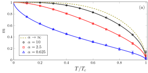
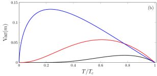
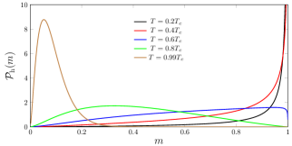
Due to the interplay between topological and thermal fluctuations, ${\rm Var}(m)$ is a non-monotonic function of $T$, with a maximum that shifts towards smaller temperatures for decreasing $\alpha$. For $0<\alpha\ll 1$, the degrees are very heterogeneous and a small amount of thermal noise leads to strong fluctuations of the local magnetizations. Figure 2 illustrates the typical shape of $\mathcal{P}_{\rm h}(m)$ for a negative binomial degree distribution and different temperatures. Similarly to the distribution of effective fields calculated in [31], the distribution $\mathcal{P}_{\rm h}(m)$ exhibits a power-law divergence at $m=0$ for $\alpha<1$, which reflects the singular behavior of the rescaled degree distribution $\nu(g)$ at $g=0$. The results in figures 1 and 2 remain qualitatively the same for the algebraic distribution of the threshold noise.

Figure 2: The stationary distribution $\mathcal{P}_{\rm h}(m)$ of local magnetizations inside the ferromagnetic phase of the Ising model on random graphs with a negative binomial degree distribution with $\alpha=2.5$ (see Eq. (32)) and the hyperbolic tangent distribution $\mu_{\rm h}$ of the threshold noise.

In the case of the hyperbolic activation function $\mathcal{F}_{\rm h}(x)$, we can expand Eqs. (38) and (39) in powers of $u$ for $0<T_{c}-T\ll 1$ and show that

$$m\simeq\pm\sqrt{\frac{3\langle G^{2}\rangle}{\langle G^{4}\rangle}}\left(\frac{T_{c}-T}{T_{c}}\right)^{\frac{1}{2}},$$ (44)

$${\rm Var}(m)\simeq\frac{3\langle G^{2}\rangle}{\langle G^{4}\rangle}\left(\langle G^{2}\rangle-1\right)\left(\frac{T_{c}-T}{T_{c}}\right),$$ (45)

where $\langle G^{n}\rangle$ is the $n$-th moment of the distribution $\nu(g)$. Consistently with previous works [8, 7, 9], Eq. (44) shows that $m$ exhibits the usual mean-field critical scaling when $\langle G^{4}\rangle$ is finite. The variance ${\rm Var}(m)$ vanishes linearly with $T_{c}-T$, analogously to the variance of the replica-symmetric effective field distribution of fully-connected spin-glass models [48].

In the case of the algebraic activation function $\mathcal{F}_{\rm a}(x)$, an expansion in powers of $u$ contains diverging coefficients, but we can still expand Eqs. (38) and (39) in powers of $u^{2\kappa}$ and derive the asymptotic behaviors

$$m\simeq\pm\left(\frac{2\kappa\langle G^{2}\rangle}{\langle G^{2\kappa+2}\rangle}\right)^{\frac{1}{2\kappa}}\left(\frac{T_{c}-T}{T_{c}}\right)^{\frac{1}{2\kappa}},$$ (46)

$${\rm Var}(m)\simeq\left(\frac{2\kappa\langle G^{2}\rangle}{\langle G^{2\kappa+2}\rangle}\right)^{\frac{1}{\kappa}}\left(\langle G^{2}\rangle-1\right)\left(\frac{T_{c}-T}{T_{c}}\right)^{\frac{1}{\kappa}}.$$ (47)

Figure 3: (a) The stationary magnetization $m$ and (b) the variance ${\rm Var}(m)$ of the distribution $\mathcal{P}_{\rm a}(m)$ of local magnetizations as a function of the reduced temperature $(T_{c}-T)/T_{c}$ (see Eq. (40)) for $\alpha=1$ and the algebraic distribution $\mu_{\rm a}$ of the threshold noise. The symbols are numerical results obtained from Eq. (43), while the dashed lines are the analytic expressions of Eqs. (46) and (47).

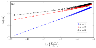
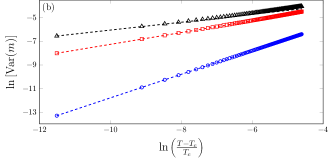
The above equations hold when $\langle G^{2\kappa+2}\rangle$ is finite. Remarkably, the critical exponents in Eqs. (46) and (47) are determined by the tails of the distribution $\mu_{\rm a}$ of the threshold noise. This is a surprising finding for a mean-field model with long-ranged interactions between the spins. Figure 3 compares Eqs. (46) and (47) with numerical solutions obtained from Eqs. (39) and (43) for different $\kappa$. The agreement between the analytic results for the critical exponents and the numerical data is excellent.

IV.2 Dynamical behavior

The nonequilibrium dynamics of the full distribution $\mathcal{P}(m,t)$ of local magnetizations is obtained by iterating Eqs. (22) and (23) from an initial condition $u(0)$, which is related to the local magnetizations $m_{1}(0),\dots,m_{N}(0)$ by means of Eq. (20). Throughout this section we consider a homogeneous initial condition $m_{i}(0)=m(0)$ ($i=1,\dots,N$), which implies that $u(0)=m(0)$. Figure 4 compares the iteration of Eqs. (19) and (22) for the average magnetization $m(t)$ with numerical simulations of Eq. (1) inside the ferromagnetic phase, confirming the exactness of the theoretical recurrence equations for $c\rightarrow\infty$. The finite-size simulation results of figure 4 converge for $t\gg 1$ to the fixed-point solutions obtained from Eqs. (38) and (39). The inset of figure 4 shows numerical simulations on random graphs generated through both the configuration model and the effective matrix of Eq. (29) for the same system size, confirming that the simulation results obtained from each method are approximately the same for large values of $N$ and $c$.

Figure 4: Dynamics of the average magnetization $m(t)$ inside the ferromagnetic phase of the Ising model on random graphs with a negative binomial degree distribution with $\alpha=0.625$. The dashed lines are derived from Eqs. (19) and (22), while the symbols are numerical simulations of Eq. (1) for $N=10^{4}$ and mean degree $c=100$. The main panel shows results for the hyperbolic tangent distribution and for the algebraic distribution (see Eq. (35)) of the threshold noise with temperature $T=T_{c}/2$. The random graphs in the numerical simulations of the main panel are sampled from Eq. (29). The inset compares numerical simulation results obtained from the configuration model and from the effective matrix of Eq. (29) for the distribution $\mu_{\rm h}$. The vertical bars are the standard deviations calculated from $10$ independent simulations.

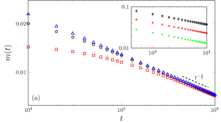
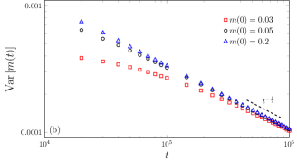
Now we discuss the nonequilibrium dynamics of $m(t)$ and ${\rm Var}\left[m(t)\right]$ at the critical temperature $T=T_{c}$. After an initial transient that depends on $m(0)$, the average magnetization $m(t)$ and the variance ${\rm Var}\left[m(t)\right]$ become independent of the initial conditions for large $t$ and they exhibit, respectively, the power-law decays

$$m(t)\propto\frac{1}{t^{z_{1}}}\quad\text{and}\quad{\rm Var}\left[m(t)\right]\propto\frac{1}{t^{z_{2}}},$$ (48)

with dynamical exponents $z_{1}$ and $z_{2}$ that only depend on the distribution of thresholds. For the algebraic distribution $\mu_{\rm a}(\zeta)$ of the threshold noise, the dynamical exponents are given by $z_{1}=1/2\kappa$ and $z_{2}=1/\kappa$, where $\kappa$ controls the power-law tails of $\mu_{\rm a}(\zeta)$. Figure 5 illustrates the critical dynamics of $m(t)$ and ${\rm Var}\left[m(t)\right]$ for $\kappa=2$. For an hyperbolic tangent distribution $\mu_{\rm h}(\zeta)$, the exponents are given by $z_{1}=1/2$ and $z_{2}=1$. These are the standard mean-field values for the critical dynamics of purely dissipative systems (models with nonconserved order-parameter) [39, 40]. Note that $z_{1}$ and $z_{2}$ have the same values as the critical indexes that govern the stationary critical behavior (see Eqs. (44-47)). The inset of figure 5-(a) clearly shows that $z_{1}$ and $z_{2}$ are independent of the variance $1/\alpha$ of the negative binomial degree distribution.

Figure 5: (a) Dynamics of the global magnetization $m(t)$ and of the (b) variance ${\rm Var}\left[m(t)\right]$ of the distribution of local magnetizations at the critical temperature $T=T_{c}$. The degrees follow a negative binomial degree distribution with relative variance $1/\alpha$. The main panels show results for $\alpha=1$, different initial conditions $m(0)$, and for the algebraic distribution $\mu_{a}(\zeta)$ of the threshold noise with $\kappa=2$. The inset in figure (a) illustrates the long-time power-law decay of $m(t)$ for $m(0)=0.4$ and different $\alpha$ (the other parameters are the same as in the main panels): $\alpha=2$ ($\diamond$), $\alpha=1$ ($\times$), and $\alpha=0.5$ ($+$).

Lastly, we investigate how degree fluctuations and the distribution of thresholds influence the dynamics of $m(t)$ inside each phase. For an arbitrary initial condition $0<m(0)<1$, the magnetization flows exponentially fast to its stationary state $m$, namely

$$|m(t)-m|\propto e^{-t/\tau}\quad(t\gg 1).$$ (49)

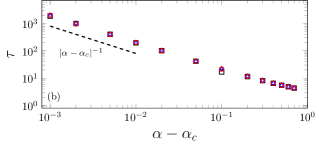
Close to a critical point, the relaxation time $\tau$ typically behaves as [10]

$$\tau\propto\xi^{Z},$$ (50)

where $\xi$ is the correlation length and $Z$ defines a dynamical exponent. In the homogeneous mean-field Ising model, the correlation length and the relaxation time diverge, respectively, as $\xi\propto|T-T_{c}|^{-1/2}$ and $\tau\propto|T-T_{c}|^{-1}$, which implies that $Z=2$ [10]. Below we examine the critical scaling of $\tau$ in the present model.

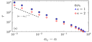
Figure 6 shows $\tau(\alpha)$ as a function of $\alpha$ for $T=2J$. As the critical value $\alpha_{c}$ is approached from each side of the transition, the relaxation time diverges as $\tau(\alpha)\propto|\alpha-\alpha_{c}|^{-1}$, independently of the distribution of thresholds. For fixed $\alpha$, $\tau(T)$ also diverges as $\tau(T)\propto|T-T_{c}|^{-1}$, regardless the shape of $\mu(\zeta)$. Thus, it is reasonable to conclude that $Z=2$ in the present model, independently of the degree distribution and of the distribution of thresholds.

Figure 6: Relaxation time $\tau$ of the average magnetization as a function of $\alpha$ for fixed temperature $T=2J$, approaching the critical value $\alpha_{c}=1$ (see Eq. (40)) from the (a) ferromagnetic and from the (b) paramagnetic phase. The quantity $1/\alpha$ is the relative variance of the negative binomial degree distribution. Each data point is obtained by fitting the long-time dynamics of $m(t)$, derived from the recurrence Eqs. (19) and (22), with the exponential function of Eq. (49).

V Final remarks

We have presented an exact solution for the dynamics of the Ising model on highly-connected random graphs with an arbitrary degree distribution. The spins are updated in parallel according to a stochastic dynamical rule which depends on a threshold noise that emulates the contact of the system with a thermal bath. For certain choices of the distribution of thresholds, the microscopic stationary states of the dynamics do not follow the Boltzmann distribution, which rules out the application of equilibrium statistical mechanics.

The solution of the model is given in terms of a general dynamical equation for the distribution of local magnetizations, which encapsulates all information about the effect of both degree and threshold fluctuations in the behavior of the system. The theoretical results for the stationary as well as for the nonequilibrium dynamics of the average magnetization have been validated by numerical simulations of the microscopic dynamics. In addition, our numerical simulations have confirmed that the interaction matrix of the Ising model on graphs sampled from the configuration model converges to the suitable matrix decomposition of Eq. (29) in the high-connectivity limit. This equation enables to simulate the Ising model on networks with an arbitrary degree distribution without resorting to more sophisticated algorithms to sample graph instances [44]. We have shown that the model undergoes a continuous transition between a paramagnetic and a ferromagnetic phase.

We have presented results for random graphs with a negative binomial degree distribution, in which the high-connectivity limit is solely parameterized by the variance of the rescaled degrees. In particular, we have focused on the critical exponents that characterize the stationary critical behavior and the long-time critical dynamics of the mean and the variance of the local magnetizations. Our main result is to show that these critical exponents depend on the distribution of the threshold noise. If the distribution of thresholds is such that the model evolves to equilibrium states, then both exponents assume their standard mean-field values [10]. In contrast, if the distribution of thresholds is such that the stationary states do not follow the Boltzmann distribution, then the aforementioned critical exponents may depend on the fluctuations of the threshold noise. Remarkably, in the case of an algebraic threshold noise both critical exponents are determined by the power-law tails of the distribution of thresholds. In addition, we have shown that the dynamical exponent for the relaxation time of the average magnetization inside each phase always assumes its standard mean-field value, regardless the distribution of the threshold noise. Overall, our results show that the details of the microscopic dynamics and the absence of detailed balance are relevant factors in determining the universality classes of spin models, in line with the critical properties of other nonequilibrium systems [10]. Still, the fact that the critical properties of the global magnetization do not belong to the mean-field universality class is somewhat surprising, given that random graphs can be seen as the infinite dimensional, mean-field limit of finite-dimensional lattices.

Although the values of all critical exponents studied here are independent of the degree fluctuations, we point out that all moments of the negative binomial degree distribution are finite. It is well established that, in the case of scale-free networks, the equilibrium critical scaling of the magnetization depends on the power-law decay of the degree distribution [9] when its fourth moment diverges. In this respect, it would be very interesting to consider the nonequilibrium dynamics of the Ising model on scale-free networks and understand whether strong degree heterogeneities are able to modify the dynamical exponents of spin models.

The probabilistic approach discussed here is general enough that it can be adapted to study the parallel as well as the sequential dynamics of other agent-based models of interacting binary variables on undirected networks [3, 37, 13, 36]. For sequential dynamics, in which a single spin is updated at each time step, there is an extra critical index that describes the short-time, non-monotonic critical dynamics of spin models [39, 49]. Our work paves the way to understand whether network heterogeneities change this critical exponent in mean-field models. We leave this and other aforementioned problems as interesting perspectives of future works.

Appendix A Solution via the generating functional approach

In this appendix we present a more rigorous derivation of Eqs. (19) and (22) based on the generating functional approach [45, 12]. The time-dependent local field is defined by Eq. (2). We assume that the entries $C_{ij}$ of the adjacency matrix $\bm{C}$ are generated according to

$$C_{ij}=\frac{c}{N}G_{i}G_{j}(1-\delta_{ij}),$$ (51)

where $G_{1},\dots,G_{N}$ are independent random variables drawn from the rescaled degree distribution $\nu(g)$. The above effective matrix $\bm{C}$ has been put forward in section III based on the asymptotic form of the local field for $c\rightarrow\infty$. Here we take Eq. (51) as the definition of the adjacency matrix elements and the starting point of our derivations, from which we will re-obtain the recurrence equation for the magnetization. The calculations in this appendix further confirm that Eq. (51) is the correct form of $\bm{C}$ for $c\rightarrow\infty$.

Our aim is to compute the disorder averaged generating functional

$$\mathcal{Z}[\bm{\psi}]= \sum_{\bm{\sigma}(0),\dots,\bm{\sigma}(t)}\exp{\left[-i\sum_{s=0}^{t}\sum_{j=1}^{N}\psi_{j}(s)\sigma_{j}(s)\right]}$$

$$\times p_{0}(\bm{\sigma}(0))\left\langle\prod_{s=0}^{t-1}W\left[\bm{\sigma}(s+1)|\bm{\sigma}(s)\right]\right\rangle_{\{G_{i}\}},$$ (52)

where $p_{0}(\bm{\sigma}(0))$ is the probability distribution of the initial state and $\langle(\dots)\rangle_{\{G_{i}\}}$ represents the average over the rescaled degrees $G_{1},\dots,G_{N}$. The derivatives of $\mathcal{Z}[\bm{\psi}]$ with respect to the auxiliary fields $\{\psi_{i}(t)\}$ yield all moments of the spin variables. For instance, the magnetization follows from

$$m(t)=\lim_{N\rightarrow\infty}\frac{i}{N}\sum_{i=1}^{N}\frac{\delta\mathcal{Z}}{\delta\psi_{i}(t)}\Bigg{|}_{\psi=0},$$ (53)

where the shorthand notation $\psi=0$ means that $\psi_{j}(s)=0$ for any $j=1,\dots,N$ and $s=0,\dots,t$.

By substituting Eq. (5) in Eq. (52), we can rewrite $\mathcal{Z}[\bm{\psi}]$ as follows

$$\mathcal{Z}[\bm{\psi}]=\sum_{\bm{\sigma}(0),\dots,\bm{\sigma}(t)}p_{0}(\bm{\sigma}(0))\,e^{-i\sum\limits_{s=0}^{t}\sum\limits_{j=1}^{N}\psi_{j}(s)\sigma_{j}(s)}$$

$$\times\int_{\mathbb{R}}\left(\prod_{j=1}^{N}\prod_{s=0}^{t-1}\frac{dh_{j}(s)d\hat{h}_{j}(s)}{4\pi}\left[1+\sigma_{j}(s+1)\mathcal{F}\left(\beta h_{j}(s)\right)\right]\right)$$

$$\times e^{i\sum\limits_{j=1}^{N}\sum\limits_{s=0}^{t-1}h_{j}(s)\hat{h}_{j}(s)}\left\langle e^{-\frac{iJ}{N}\sum\limits_{s=0}^{t-1}\sum\limits_{jk=1}^{N}G_{j}G_{k}\hat{h}_{j}(s)\sigma_{k}(s)}\right\rangle_{\{G_{i}\}},$$ (54)

in which the integration variables $\{h_{j}(s),\hat{h}_{j}(s)\}$ have been introduced through Dirac $\delta$-functions [12]. In order to perform the average over $G_{1},\dots,G_{N}$, we need to decouple sites in the exponent of the above equation, which is achieved by inserting the macroscopic order-parameters

$$u(s)=\frac{1}{N}\sum\limits_{i=1}^{N}G_{i}\sigma_{i}(s)$$

and

$$v(s)=\frac{1}{N}\sum\limits_{i=1}^{N}G_{i}\hat{h}_{i}(s)$$

via Dirac $\delta$-functions that enforce the above definitions. Moreover, by assuming that the initial states of the spins are independent, $p_{0}(\bm{\sigma}(0))=\prod_{i=1}^{N}p_{0}(\sigma_{i}(0))$, the computation of $\mathcal{Z}[\bm{\psi}]$ can be recast in terms of the calculation of an integral over the order-parameters and its conjugate variables $\{\hat{u}(s),\hat{v}(s)\}$, namely

$$\mathcal{Z}[\bm{\psi}]=\int\limits_{\mathbb{R}}\left(\prod\limits_{s=0}^{t-1}\frac{N^{2}du(s)dv(s)d\hat{u}(s)d\hat{v}(s)}{4\pi^{2}}\right)e^{N\Phi[u,v,\hat{u},\hat{v}]}.$$ (55)

The functional $\Phi[u,v,\hat{u},\hat{v}]$ is given by

$$\Phi[u,v,\hat{u},\hat{v}] =i\sum\limits_{s=0}^{t-1}\left[u(s)\hat{u}(s)+v(s)\hat{v}(s)-Ju(s)v(s)\right]$$

$$+\frac{1}{N}\sum\limits_{j=1}^{N}\ln\Bigg{\{}\sum\limits_{\vec{\sigma}}\int_{\mathbb{R}}\frac{d\vec{h}d\vec{\hat{h}}}{(2\pi)^{t}}e^{-i\sum\limits_{s=0}^{t}\psi_{j}(s)\sigma(s)}$$

$$\times\left\langle\mathcal{M}_{G}\left(\vec{h},\vec{\hat{h}},\vec{\sigma}\right)\right\rangle_{G}\Bigg{\}},$$ (56)

where $d\vec{h}d\vec{\hat{h}}=\prod\limits_{s=0}^{t-1}dh(s)d\hat{h}(s)$ and

$$\mathcal{M}_{G}\left(\vec{h},\vec{\hat{h}},\vec{\sigma}\right)=p_{0}(\sigma(0))\prod_{s=0}^{t-1}\frac{1}{2}\left[1+\sigma(s+1)\mathcal{F}\left(\beta h(s)\right)\right]$$

$$e^{i\sum\limits_{s=0}^{t-1}h(s)\hat{h}(s)-iG\sum\limits_{s=0}^{t-1}\hat{u}(s)\sigma(s)-iG\sum\limits_{s=0}^{t-1}\hat{v}(s)\hat{h}(s)}.$$ (57)

Note that we have defined the vectors $\vec{\sigma}=(\sigma(0),\dots,\sigma(t))^{T}$, $\vec{h}=(h(0),\dots,h(t-1))^{T}$, and $\vec{\hat{h}}=(\hat{h}(0),\dots,\hat{h}(t-1))^{T}$, which reflects the reduction of the computation of $\mathcal{Z}[\bm{\psi}]$ to an effective single-spin problem.

In the limit $N\rightarrow\infty$, the integral in Eq. (55) is solved by the saddle-point method and the generating functional reads

$$\mathcal{Z}[\bm{\psi}]\simeq\exp{\left(N\Phi_{*}[u,v,\hat{u},\hat{v}]\right)},$$ (58)

where $\Phi_{*}[u,v,\hat{u},\hat{v}]$ is the stationary value of $\Phi$. By deriving the functional $\Phi[u,v,\hat{u},\hat{v}]$ with respect to its arguments and then setting $\psi=0$, we obtain the saddle-point equations for the order-parameters and their conjugate variables,

$$\hat{u}(l)=Jv(l),$$ (59)

$$\hat{v}(l)=Ju(l),$$ (60)

$$u(l)=\frac{\sum\limits_{\vec{\sigma}}\int_{\mathbb{R}}d\vec{h}d\vec{\hat{h}}\,\sigma(l)\left\langle G\mathcal{M}_{G}\left(\vec{h},\vec{\hat{h}},\vec{\sigma}\right)\right\rangle_{G}}{\sum\limits_{\vec{\sigma}}\int_{\mathbb{R}}d\vec{h}d\vec{\hat{h}}\left\langle\mathcal{M}_{G}\left(\vec{h},\vec{\hat{h}},\vec{\sigma}\right)\right\rangle_{G}},$$ (61)

$$v(l)=\frac{\sum\limits_{\vec{\sigma}}\int_{\mathbb{R}}d\vec{h}d\vec{\hat{h}}\,\hat{h}(l)\left\langle G\mathcal{M}_{G}\left(\vec{h},\vec{\hat{h}},\vec{\sigma}\right)\right\rangle_{G}}{\sum\limits_{\vec{\sigma}}\int_{\mathbb{R}}d\vec{h}d\vec{\hat{h}}\left\langle\mathcal{M}_{G}\left(\vec{h},\vec{\hat{h}},\vec{\sigma}\right)\right\rangle_{G}},$$ (62)

which give the arguments of $\Phi_{*}[u,v,\hat{u},\hat{v}]$. The magnetization

$$m(t)=\frac{\sum\limits_{\vec{\sigma}}\int_{\mathbb{R}}d\vec{h}d\vec{\hat{h}}\,\sigma(t)\left\langle\mathcal{M}_{G}\left(\vec{h},\vec{\hat{h}},\vec{\sigma}\right)\right\rangle_{G}}{\sum\limits_{\vec{\sigma}}\int_{\mathbb{R}}d\vec{h}d\vec{\hat{h}}\left\langle\mathcal{M}_{G}\left(\vec{h},\vec{\hat{h}},\vec{\sigma}\right)\right\rangle_{G}}$$ (63)

is obtained from Eqs. (53) and (58).

The last step consists in simplifying the saddle-point equations. By adding a term of the form $G_{j}\theta_{j}(s)$ to the local field, Eq. (2), and then performing the same calculation that led us to the above saddle-point integral, one finds that the single-site conjugate fields $\{\hat{h}(s)\}$ couple to the external fields $\{\theta_{j}(s)\}$ in such a way that the order-parameter $v(s)$ can be written in terms of the derivatives $\frac{\delta\mathcal{Z}}{\delta\theta_{j}(s)}\Big{|}_{\psi=0}$. Combining this fact with the normalization property $\mathcal{Z}[0]=1$, one can show that $v(s)=0\,\,\forall\,s$, which leads to the following expression for the magnetization

$$m(t) =\int_{\mathbb{R}}\frac{d\vec{h}d\vec{\hat{h}}}{(2\pi)^{t}}\left\langle e^{i\sum\limits_{s=0}^{t-1}\hat{h}(s)\left[h(s)-GJu(s)\right]}\right\rangle_{G}$$

$$\times\sum_{\vec{\sigma}}p_{0}(\sigma(0))\sigma(t)\prod_{s=0}^{t-1}\frac{1}{2}\left[1+\sigma(s+1)\mathcal{F}\left(\beta h(s)\right)\right]$$ (64)

and for the order-parameter $u(t)$

$$u(t) =\int_{\mathbb{R}}\frac{d\vec{h}d\vec{\hat{h}}}{(2\pi)^{t}}\left\langle G\,e^{i\sum\limits_{s=0}^{t-1}\hat{h}(s)\left[h(s)-GJu(s)\right]}\right\rangle_{G}$$

$$\times\sum_{\vec{\sigma}}p_{0}(\sigma(0))\sigma(t)\prod_{s=0}^{t-1}\frac{1}{2}\left[1+\sigma(s+1)\mathcal{F}\left(\beta h(s)\right)\right].$$ (65)

Recalling that the random variable $G$ follows from the distribution $\nu(g)$, it is straightforward to recover Eqs. (19) and (22) by performing the sum over $\vec{\sigma}$ and the integrals over the fields in the above expressions.

References

- Dorogovtsev et al. [2008] S. N. Dorogovtsev, A. V. Goltsev, and J. F. F. Mendes, “Critical phenomena in complex networks,” Rev. Mod. Phys. 80, 1275–1335 (2008).
- Barrat et al. [2008] A. Barrat, M. Barthélemy, and A. Vespignani, Dynamical Processes on Complex Networks (Cambridge University Press, 2008).
- Castellano et al. [2009] Claudio Castellano, Santo Fortunato, and Vittorio Loreto, “Statistical physics of social dynamics,” Rev. Mod. Phys. 81, 591 (2009).
- Mézard and Montanari [2009] M. Mézard and A. Montanari, Information, Physics, and Computation (Oxford University Press, 2009).
- Newman et al. [2001] M. E. J. Newman, S. H. Strogatz, and D. J. Watts, “Random graphs with arbitrary degree distributions and their applications,” Phys. Rev. E 64, 026118 (2001).
- Cardy et al. [1996] J. Cardy, P. Goddard, and J. Yeomans, Scaling and Renormalization in Statistical Physics, Cambridge Lecture Notes in Physics (Cambridge University Press, 1996).
- Leone et al. [2002] M. Leone, A. Vázquez, A. Vespignani, and R. Zecchina, “Ferromagnetic ordering in graphs with arbitrary degree distribution,” Eur. Phys. J. B 28, 191 (2002).
- Dorogovtsev et al. [2002] S. N. Dorogovtsev, A. V. Goltsev, and J. F. F. Mendes, “Ising model on networks with an arbitrary distribution of connections,” Phys. Rev. E 66, 016104 (2002).
- Dommers et al. [2016] S. Dommers, C. Giardinà, C. Giberti, R. van der Hofstad, and M. L. Prioriello, “Ising critical behavior of inhomogeneous curie-weiss models and annealed random graphs,” Commun. Math. Phys. 348, 221 (2016).
- Ódor [2004] Géza Ódor, “Universality classes in nonequilibrium lattice systems,” Rev. Mod. Phys. 76, 663–724 (2004).
- Coolen [2001a] A.C.C. Coolen, “Chapter 14 statistical mechanics of recurrent neural networks i—statics,” in Neuro-Informatics and Neural Modelling, Handbook of Biological Physics, Vol. 4, edited by F. Moss and S. Gielen (North-Holland, 2001) p. 553.
- Coolen [2001b] A.C.C. Coolen, “Chapter 15 statistical mechanics of recurrent neural networks ii — dynamics,” in Neuro-Informatics and Neural Modelling, Handbook of Biological Physics, Vol. 4, edited by F. Moss and S. Gielen (North-Holland, 2001) p. 619.
- Torrisi et al. [2022] Giuseppe Torrisi, Reimer Kühn, and Alessia Annibale, “Uncovering the non-equilibrium stationary properties in sparse boolean networks,” Journal of Statistical Mechanics: Theory and Experiment 2022, 053303 (2022).
- Hatchett et al. [2004] J P L Hatchett, B Wemmenhove, I Pérez Castillo, T Nikoletopoulos, N S Skantzos, and A C C Coolen, “Parallel dynamics of disordered ising spin systems on finitely connected random graphs,” Journal of Physics A: Mathematical and General 37, 6201 (2004).
- Mimura and Coolen [2009] Kazushi Mimura and A C C Coolen, “Parallel dynamics of disordered ising spin systems on finitely connected directed random graphs with arbitrary degree distributions,” Journal of Physics A: Mathematical and Theoretical 42, 415001 (2009).
- Neri and Bollé [2009] I Neri and D Bollé, “The cavity approach to parallel dynamics of ising spins on a graph,” Journal of Statistical Mechanics: Theory and Experiment 2009, P08009 (2009).
- Mozeika and Coolen [2008] A. Mozeika and A. C. C. Coolen, “Dynamical replica analysis of processes on finitely connected random graphs: I. vertex covering,” Journal of Physics A: Mathematical and Theoretical 41, 115003 (2008).
- Metz and Theumann [2008] F L Metz and W K Theumann, “Instability of frozen-in states in synchronous hebbian neural networks,” Journal of Physics A: Mathematical and Theoretical 41, 265001 (2008).
- Del Ferraro and Aurell [2015] Gino Del Ferraro and Erik Aurell, “Dynamic message-passing approach for kinetic spin models with reversible dynamics,” Phys. Rev. E 92, 010102 (2015).
- Aurell et al. [2017] E. Aurell, G. Del Ferraro, E. Domínguez, and R. Mulet, “Cavity master equation for the continuous time dynamics of discrete-spin models,” Phys. Rev. E 95, 052119 (2017).
- Roudi and Hertz [2011a] Yasser Roudi and John Hertz, “Mean field theory for nonequilibrium network reconstruction,” Phys. Rev. Lett. 106, 048702 (2011a).
- Roudi and Hertz [2011b] Yasser Roudi and John Hertz, “Dynamical tap equations for non-equilibrium ising spin glasses,” Journal of Statistical Mechanics: Theory and Experiment 2011, P03031 (2011b).
- Aurell and Mahmoudi [2012] Erik Aurell and Hamed Mahmoudi, “Dynamic mean-field and cavity methods for diluted ising systems,” Phys. Rev. E 85, 031119 (2012).
- Pelizzola [2013] A. Pelizzola, “Variational approximations for stationary states of ising-like models,” Eur. Phys. J. B 86, 120 (2013).
- Vázquez et al. [2017] Eduardo Domínguez Vázquez, Gino Del Ferraro, and Federico Ricci-Tersenghi, “A simple analytical description of the non-stationary dynamics in ising spin systems,” Journal of Statistical Mechanics: Theory and Experiment 2017, 033303 (2017).
- Derrida et al. [1987] B. Derrida, E. Gardner, and A. Zippelius, “An exactly solvable asymmetric neural network model,” Europhysics Letters 4, 167 (1987).
- Mézard and Parisi [2001] M. Mézard and G. Parisi, “The bethe lattice spin glass revisited,” Eur. Phys. J. B 20, 217 (2001).
- Mézard and Parisi [2003] M. Mézard and G. Parisi, “The cavity method at zero temperature,” J. Stat. Phys. 111, 1 (2003).
- Metz and Silva [2020] Fernando L. Metz and Jeferson D. Silva, “Spectral density of dense random networks and the breakdown of the wigner semicircle law,” Phys. Rev. Research 2, 043116 (2020).
- Silva and Metz [2022] Jeferson D. Silva and Fernando L. Metz, “Analytic solution of the resolvent equations for heterogeneous random graphs: spectral and localization properties,” (2022).
- Metz and Peron [2022] Fernando L Metz and Thomas Peron, “Mean-field theory of vector spin models on networks with arbitrary degree distributions,” Journal of Physics: Complexity 3, 015008 (2022).
- Kanoria and Montanari [2011] Yashodhan Kanoria and Andrea Montanari, “Majority dynamics on trees and the dynamic cavity method,” The Annals of Applied Probability 21, 1694 – 1748 (2011).
- Holehouse and Moran [2022] James Holehouse and José Moran, “Exact time-dependent dynamics of discrete binary choice models,” Journal of Physics: Complexity 3, 035005 (2022).
- Kauffman [1969] S.A. Kauffman, “Metabolic stability and epigenesis in randomly constructed genetic nets,” Journal of Theoretical Biology 22, 437–467 (1969).
- Mozeika and Saad [2011] Alexander Mozeika and David Saad, “Dynamics of boolean networks: An exact solution,” Phys. Rev. Lett. 106, 214101 (2011).
- Hurry et al. [2022] Christian John Hurry, Alexander Mozeika, and Alessia Annibale, “Dynamics of sparse boolean networks with multi-node and self-interactions,” Journal of Physics A: Mathematical and Theoretical 55, 415003 (2022).
- Bouchaud [2013] Jean-Philippe Bouchaud, “Crises and collective socio-economic phenomena: Simple models and challenges,” J. Stat. Phys. 151, 567 (2013).
- Peretto [1984] P. Peretto, “Collective properties of neural networks: A statistical physics approach,” Biol. Cybern. 50, 51 (1984).
- Janssen et al. [1989] H.K. Janssen, B. Schaub, and B. Schmittmann, “New universal short-time scaling behaviour of critical relaxation processes,” Z. Physik B 73, 539 (1989).
- Calabrese and Gambassi [2005] Pasquale Calabrese and Andrea Gambassi, “Ageing properties of critical systems,” Journal of Physics A: Mathematical and General 38, R133 (2005).
- Adzhemyan et al. [2022] L.Ts. Adzhemyan, D.A. Evdokimov, M. Hnatič, E.V. Ivanova, M.V. Kompaniets, A. Kudlis, and D.V. Zakharov, “The dynamic critical exponent z for 2d and 3d ising models from five-loop epsilon expansion,” Physics Letters A 425, 127870 (2022).
- Bollobás [2001] B. Bollobás, Random Graphs, Cambridge Studies in Advanced Mathematics (Cambridge University Press, 2001).
- Molloy and Reed [1995] Michael Molloy and Bruce Reed, “A critical point for random graphs with a given degree sequence,” Random Structures & Algorithms 6, 161 (1995).
- Fosdick et al. [2018] Bailey K. Fosdick, Daniel B. Larremore, Joel Nishimura, and Johan Ugander, “Configuring random graph models with fixed degree sequences,” SIAM Review 60, 315 (2018).
- Martin et al. [1973] P. C. Martin, E. D. Siggia, and H. A. Rose, “Statistical dynamics of classical systems,” Phys. Rev. A 8, 423 (1973).
- Coolen et al. [2017] A.C.C. Coolen, A. Annibale, and E. Roberts, Generating Random Networks and Graphs (Oxford University Press, 2017).
- Kochmański et al. [2013] M Kochmański, T Paszkiewicz, and S Wolski, “Curie–weiss magnet—a simple model of phase transition,” European Journal of Physics 34, 1555 (2013).
- Sherrington and Kirkpatrick [1975] David Sherrington and Scott Kirkpatrick, “Solvable model of a spin-glass,” Phys. Rev. Lett. 35, 1792 (1975).
- Anteneodo et al. [2010] Celia Anteneodo, Ezequiel E Ferrero, and Sergio A Cannas, “Short-time dynamics of finite-size mean-field systems,” Journal of Statistical Mechanics: Theory and Experiment 2010, P07026 (2010).