Human in the loop: How to effectively create coherent topics by manually labeling only a few documents per class

Abstract

Few-shot methods for accurate modeling under sparse label-settings have improved significantly. However, the applications of few-shot modeling in natural language processing remain solely in the field of document classification. With recent performance improvements, supervised few-shot methods, combined with a simple topic extraction method pose a significant challenge to unsupervised topic modeling methods. Our research shows that supervised few-shot learning, combined with a simple topic extraction method, can outperform unsupervised topic modeling techniques in terms of generating coherent topics, even when only a few labeled documents per class are used.

1 Introduction

The identification of latent topics in large text corpora has undergone a great deal of development. However, uncovering the hidden semantics of large text corpora is still, if not of ever-increasing interest. Scientific methods continue to evolve and achieve increasingly impressive results in terms of topic coherence (Larochelle and Lauly, 2012; Srivastava and Sutton, 2017; Chien et al., 2018; Wang et al., 2019; Dieng et al., 2020). The practical relevance of such methods is evident from the large number of practical application papers alone. Topic models for information extraction are used, for example, for applied research in education (Granić and Marangunić, 2019), offsite construction (Liu et al., 2019a), bioinformatics (Liu et al., 2016), communication sciences (Maier et al., 2018) and many other practical areas (e.g. (Hall et al., 2008; Daud et al., 2010; Boyd-Graber et al., 2017; Jelodar et al., 2019; Hannigan et al., 2019)).

While all of these methods take an unsupervised approach, few-shot methods achieve remarkable results in various supervised label-scarse settings. The metrics of interest are in this case not the coherence of clusters, but model accuracy, F1 score, or precision. Huggingfaces Sentence Transformer Finetuning (SetFit) (Tunstall et al., 2022) allows for such a small amount of labeled data while achieving impressive classification results that unsupervised methods are heavily challenged.

The idea is simple. When less and less labeled documents per class are necessary for supervised methods to achieve state-of-the-art results, human input by manually labeling a few documents becomes an attractive option for unsupervised tasks such as document clustering. By leveraging pre-trained sentence transformers (Reimers and Gurevych, 2019) and class-based term frequency inverse document frequency (tf-idf) for topic extraction, we can generate coherent topics with only a few labeled documents per class. As a result, manually labeling a training data set and subsequently leveraging SetFit reduces the tiresome and time- and money-intensive manual labeling by such a dramatic amount, that it is a viable alternative to unsupervised approaches.

Contributions

The contributions of the paper can be summarized as follows:

1. We present a method for Document Classification and subsequent Topic Extraction (DCTE) based on SetFit. The proposed method generates coherent topics from only a few labeled documents.

2. We conduct a benchmark study, comparing the proposed approach with state-of-the-art topic models and document clustering methods.

3. We outperform competitive benchmark models on three standard datasets in terms of topic coherence and create informative topics.

2 Related Work and Background

Generative probabilistic models inspired by Latent Dirichlet Allocation (LDA) Blei et al. (2003) topic models are still widely used. Several extensions, heavily drawing from LDA and also leveraging word-embeddings achieve state of the art results in terms of coherence Wang et al. (2019); Dieng et al. (2020). Based upon Srivastava and Sutton (2017), Bianchi et al. (2021) introduce the Zero-shot Topic model, which enables zero-shot cross lingual tasks. Word-, document- and sentence- embeddings generated such a great performance impact, that even structurally simple models, leveraging pre-trained word- and sentence-embeddings and clustering these embeddings achieve remarkable results Grootendorst (2022); Sia et al. (2020); Angelov (2020). The embedding types range from doc2vec Le and Mikolov (2014) over sentence-transformers (Reimers and Gurevych, 2019, 2020) to word-embeddings generated with BERT Devlin et al. (2018); Liu et al. (2019b). Modeling techniques include K-Means, Hierarchical Density-Based Spatial Clustering of Applications with Noise (HDBSCAN) McInnes et al. (2017) and Gaussian Mixture Models (GMM) Reynolds (2009). Topics are extracted with class based tf-idf Grootendorst (2022) or based on distance measures in the feature space Angelov (2020); Sia et al. (2020). Leveraging pre-trained embeddings from large scale language models seems to positively impact modeling performance Bianchi et al. (2020).

The inclusion of labeled data into topic modeling was mostly done to improve unsupervised results in text mining (Ramage et al., 2011) and for multi-labeled corpora (Ramage et al., 2009). Few-shot topic modeling has only been of interest as of late (Iwata, 2021; Duan et al., 2022). Iwata (2021) introduces a few-shot model that relies on a neural network generating priors for generative probabilistic topic modeling and achieves impressive results with respect to perplexity. Duan et al. (2022) introduces a bi-level generative model combined with a topic-meta learner. However, both few-shot methods are designed to create great topics from little data. A setting that is exceedingly unlikely given the ever growing availability of large text corpora. In contrast, leveraging existing few-shot methods for generating coherent topics for very small samples of labeled training data has a high practical relevance. When only a handful of documents have to be labeled manually to improve topic coherence, creating humanly labeled training data is a viable and effective option.

SetFit

The leveraged model, SetFit (Tunstall et al., 2022), can be described as a two-step algorithm. In a first step, an already pre-trained Sentence Transformer Reimers and Gurevych (2019) is fine-tuned using only a few-labeled samples per class. A siamese, contrastive architecture is used on sentence/document pairs to ensure better generalizability. Creating these contrastive learning pairs artificially enlarges the training data set. The size of this fine-tuning dataset is therefore dependent on the number of labeled training sentences and classes. For $k$ classes and $n$ equally distributed samples per class, we can hence construct $\sum_{i=1}^{k-1}n(k-i)n$ contrastive learning pairs. Each contrastive learning pair thus consist of one positive sample from class $c$ and one randomly selected negative sample from a different class. This contrastive architecture increases the small amount of training data by a margin and enables the model to achieve the impressive classification results with extremely little data as shown by Tunstall et al. (2022). Second, a classification head is trained using the encoded training corpus.

3 Methodology

Our proposed methodology is surprisingly simple, yet highly effective. Let the vocabulary of words be expressed as $\textup{V}=\left\{w_{1},~{}\ldots~{},w_{n}\right\}$. Let the corpus, i.e. the collection of documents be expressed as $\textup{D}=\left\{d_{1},~{}\ldots~{},d_{M}\right\}$. Further, let each document be expressed as a sequence of words $d_{i}=\left[w_{i1},\ldots,w_{in_{i}}\right]$ where $w_{ij}\in V$ and $n_{i}$ denotes the length of document $d_{i}$. $\mathcal{D}=\left\{\bm{\delta}_{1},~{}\ldots~{},\bm{\delta}_{M}\right\}$ then denotes the set of documents represented in the embedding space, such that $\bm{\delta}_{i}$ is the vector representation of $d_{i}$. Further, let a topic $t_{k}$ from a set of topics $T=\left\{t_{1},~{}\ldots~{},t_{K}\right\}$ be represented as a discrete probability distribution over the vocabulary (Blei et al., 2003), such that $t_{k}$ is expressed as $(\phi_{k,1},\ldots,\phi_{k,n})^{T}$ and $\sum_{i=1}^{n}\phi_{k,i}=1$ for every $k$.

Figure 1: The models average classification accuracies dependent on the number of labeled training samples. As expected, the accuracy increases with the number of labeled samples. i denotes the number of classes present in the dataset. Each model is fit 5 times, using different randomly selected documents in the training corpus. We find that a model’s coherence and a model’s accuracy are independent from another (see Table 3).

To generate topics, we fine-tune a Sentence-Transformer Reimers and Gurevych (2019) leveraging the SetFit architecture. Subsequently, we train a classification head on the fine-tuned document embeddings $\mathcal{D}$. Using a Neural Network and bypassing classical unsupervised clustering allows to circumvent dimensionality reduction as opposed to Sia et al. (2020); Grootendorst (2022) or Angelov (2020). As Deep neural networks are not susceptible to a dimensionality curse, no information is lost during a dimensionality reduction step. The classification head is trained only with the few labeled samples. The remaining documents are mapped into the embedding space and classified. Subsequently, the topics are extracted from the resulting document clusters.

Topic Extraction

As the proposed method only results in document clusters, but not a set of topics $T$, we must extract the topics from the document clusters. We use a method already proven successful in the literature, the class-based tf-idf approach (Salton, 1989; Grootendorst, 2022),

$$\mbox{tf-idf}(w|c)=\frac{frequency(w_{c})}{n_{c}}\cdot\log\left(\frac{N}{\sum_{j}w_{j}}\right).$$

With $frequency(w_{c})$ being the total frequency of the word in class $c$, $n_{c}$ being the total number of words in class $c$, N being the total number of documents and $\sum_{j}w_{j}$ being the overall frequency of word $w$ over all classes. A topic, $t_{k}$ is hence represented by the top $j$ words according to the words normalized tf-idf scores.

	Random draw				Per class
	Samples	Average	Max	Std.	Samples	Average	Max	Std.
20 News- groups	20	0.185	0.221	$\pm$0.080	1	0.117	0.163	$\pm$0.036
	40	0.108	0.144	$\pm$0.024	2	0.115	0.196	$\pm$0.046
	60	0.122	0.190	$\pm$0.032	3	0.137	0.189	$\pm$0.061
	80	0.145	0.190	$\pm$0.045	4	0.186	0.208	$\pm$0.021
	100	0.162	0.200	$\pm$0.047	5	0.164	0.192	$\pm$0.027
BBC News	5	0.097	0.20	$\pm$0.084	1	0.103	0.153	$\pm$0.032
	10	0.192	0.152	$\pm$0.059	2	0.133	0.187	$\pm$0.047
	15	0.115	0.124	$\pm$0.054	3	0.107	0.180	$\pm$0.041
	20	0.081	0.139	$\pm$0.024	4	0.117	0.191	$\pm$0.040
	25	0.121	0.115	$\pm$0.020	5	0.142	0.186	$\pm$0.022
M10	10	-0.178	-0.015	$\pm$0.119	1	-0.146	-0.078	$\pm$0.037
	20	-0.153	-0.12	$\pm$0.021	2	-0.115	-0.054	$\pm$0.039
	30	-0.142	-0.078	$\pm$0.033	3	-0.158	-0.107	$\pm$0.032
	40	-0.098	-0.033	$\pm$0.055	4	-0.119	-0.103	$\pm$0.015
	50	-0.094	-0.054	$\pm$0.035	5	-0.121	-0.098	$\pm$0.027

Table 1: Experimental results for different numbers of labeled training samples. The average NPMI coherence and standard deviations over 5 runs is presented. All models are fit using the all-MiniLM-L6-v2 sentence transformer. The biggest coherence score for each column for each dataset is marked in bold.

4 Experiments

Evaluation

To evaluate the topics, we use normalised pointwise mutual information (NPMI) coherence scores (Lau et al., 2014).

$$NPMI(t_{k})=\sum_{j=2}^{N}\sum_{i=1}^{j-1}\frac{log\frac{(P(w_{i},w_{j})}{P(w_{i})P(w_{j})}}{-log(P(w_{i},w_{j})}$$

We use the training corpora as the reference corpora for constructing coherence scores respectively. Stopwords are removed to punish models that include meaningless words into their topics more severely and not favor models constructing information-less topics with frequently co-occurring words. $N$ is set to 10 for all evaluations over all models.

Experimental setup

We use the 20 Newsgroups, BBC News and M10 corpora as the benchmark datasets. To circumvent any induced bias in the results by a lucky selection of labeled training documents, we train the model several times, each time with different randomly selected labeled training documents. All topics are evaluated with coherence scores. We compare the results with state-of-the-art unsupervised topic modeling and document clustering approaches. To achieve the best possible comparability we choose the same pre-trained sentence-transformer, all-MiniLM-L6-v2 (Reimers and Gurevych, 2019), for all benchmark models where applicable. All models are fit using the OCTIS framework (Terragni et al., 2021). A detailed description of the models hyperparameters and the hyperparameter tuning can be found in the Appendix, B.

For DCTE we compare two different labeling frameworks. One, which uses $n=1,\dots,5$ labeled randomly drawn documents per class and one where we use $i$ randomly labeled documents without correcting for true labels, with $i$ being dependent on the dataset. $i=20,40,\dots,100$ for 20 Newsgroups, $i=5,10,\dots,25$ for BBC News and $i=10,20,\dots,50$ for M10. Note, that we perform hyperparameter tuning for all benchmark models (see Appendix, B), but use a vanilla approach for DCTE. This demonstrates a useful real-world applicability as the method generates coherent topics out of the box and independent of the dataset or even the selected training samples (see Table 3).

Results

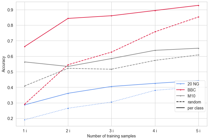
The results for the proposed approach can be seen in table 3. We find that even with a small amount of labeled data, coherent topics can be constructed. The coherence does not depend on the number of training samples and one labeled document per class is sufficient to create coherent topics. When randomly drawing from the corpus, we find larger standard deviations in the average coherence scores over 5 runs. This is due to the fact that with random sampling, one might fail to include all classes present in the dataset into the training data. This is also represented by the poor classification accuracies represented in Figure 1. However, we find that even under these conditions, coherent topics are created. Table 3 shows the performance compared to the benchmark models. Additionally, we find that the presented method not only creates coherent but also informative topics (See Appendix, tables 3 - 4). Even with these few labeled training samples per class, DCTE creates coherent topics. The use of supervised methods and especially the lack of any form of dimensionality reduction seem to have a positive effect on topic coherence.

5 Conclusion

In this paper, we show that recent improvements in few-shot models make manual labeling of a few training documents a valid alternative to unsupervised topic modeling. With a small amount of human input in the form of labeled training samples, even simple topic extraction methods can yield great results in terms of topic coherence. Additionally, the achieved coherence scores are achieved without any form of hyperparameter tuning and relatively low number of epochs and text pairs for the contrastive learning (Appendix, B). While already achieving great coherence scores, this leaves further possibilities for improvement in the presented method. Furthermore, we find that the created document-topic distributions match the underlying distributions in the dataset (Appendix, D).

¹ The most coherent model, using 20, 5 and 10 randomly drawn labeled training samples respectively. ² The best model achieved with only one labeled training sample per class. ³ The average achieved coherence when using only one labeled training sample per class. ⁴ The average achieved coherence when using 4 labeled training samples per class.

Table 2: NPMI coherence scores for all tested models on the three benchmark datasets. CTM, BERTopic, K-Means and SetFit are all fit using all-MiniLM-L6-v2 (Reimers and Gurevych, 2019). LDA is fit using standard bag-of-words representations. NeuralLDA and ETM are fit using Word2Vec (Mikolov et al., 2013) As BERTopic uses HDBSCAN, it detects the number of topics automatically. However, it drastically overestimates the number of true topics for all datasets. To account for garbage topics negatively impacting the coherence scores, we favorably choose to also evaluate only the top 50 % coherent topics from that output. The top four coherent models are marked in bold.

6 Limitations

While there are multiple advantages of the presented method there are also apparent limitations. Although we can effectively generate coherent topics with a very small amount of labeled data, it still requires manual labeling. Additionally, manual labeling requires an idea of how many different topics are present in the corpus. However, most unsupervised methods also require setting a fixed number of topics Blei et al. (2003); Sia et al. (2020); Dieng et al. (2020). Moreover, most algorithms optimize the number of extracted topics over coherence scores, which could easily be done with the presented method. Note that the presented benchmarks for DCTE are all achieved without any form of hyperparameter tuning. This reduces computation time and artificially creates an idea of how real-world applications could benefit from this method. This paper does not delve into results from different few-shot document classifiers, (e.g.(Rios and Kavuluru, 2018; Pan et al., 2019; Cao et al., 2020)) or different pre-trained sentence transformers for document embeddings (Reimers and Gurevych, 2019). Future research may implement additional few-shot methods to potentially find even better suited few-shot classifiers and embedding models for creating coherent topics.

Besides, additional applications could include multi-labeled and multi-topic documents. Both of these problems can be easily solved with the presented method. The topic extraction method could be replaced by a similar method as used by Sia et al. (2020). Topical centroids could be constructed and distance measures in the embedding space could be used to extract the topics (see Appendix, A).

Appendix A Appendix

Topic Extraction

Another method for topic extraction could be adapted from Angelov (2020) and Sia et al. (2020). In this approach, document clusters are first represented as topical centroids in the embedding space, $\bm{\mu}$. This allows for soft-clustering and hence multi-labeled documents, but requires additional computation steps and can be susceptible to a chosen embedding model. Second, the vocabulary $\textup{V}=\left\{w_{1},~{}\ldots~{},w_{n}\right\}$ is also mapped into the same feature space, such that $\mathcal{W}=\left\{\bm{\omega}_{1},~{}\ldots~{},\bm{\omega}_{n}\right\}$. Hence, each word $w_{i}$ in the embedding space represented as $\bm{\omega}_{i}\in\mathbb{R}^{L}$ has the same dimensionality $L$ as a document vector $\bm{\delta}_{i}\in\mathbb{R}^{L}$. There are two ways to represent a document as an average over word-embeddings. First, using the approach from Sia et al. (2020), which involves representing a document as an average of word-embeddings created with BERT (Devlin et al., 2018). Second, interpreting the vocabulary as one-word sentences and using the same embedding model as for the documents. Subsequently, the similarity between every word and every topical centroid is computed e.g. as:

$$sim(\bm{\omega},\bm{\mu})=\frac{\bm{\omega}\cdot\bm{\mu}}{\lVert\bm{\omega}\rVert\|\bm{\mu}\lVert},$$

where ω ⋅μ=∑_i=1^L ω_i μ_i and ∥ω∥∥μ∥=∑_i=1^L (ω_i)^2 ∑_i=1^L (μ_i)^2. $L$ denotes the vectors dimension in the feature space, which is identical for $\bm{\omega}$ and $\bm{\mu}$.

Appendix B Experimental Details

All benchmark models are fitted 5 times for each dataset. The reported coherence scores are favorably the maximum coherence score achieved of the model during the 5 runs.

All benchmark models are fitted using the same pre-trained Sentence Transformer, all-MiniLM-L6-v2 (Reimers and Gurevych, 2019), when applicable. The dimensionality reduction of the embedding in BERTopic (Grootendorst, 2022) is set as the default. Hence, the embeddings are reduced to 5 dimensions using umap (McInnes et al., 2018). As intended by the author, HDBSCAN (McInnes et al., 2017) is used for clustering. Because the number of clusters is detected automatically in HDBSCAN and we find that BERTopic heavily overestimates the number of true classes in the dataset, we report both, first the average coherence score over all topics and second the average coherence score for the top 50% coherent topics. For the K-Means application, we closely follow the approach by Grootendorst (2022), but change HDBSCAN to the K-Means algorithm, such that we can fix the number of topics manually. For dimensionality reduction, we optimize with respect to coherence scores and test a range from 2, to 20, using umap. We use 15 dimensions for all three datasets, as 15 dimensions performed marginally favorably compared to the 5 dimensions used in BERTopic Grootendorst (2022) and Angelov (2020). We additionally tested the Top2Vec model (Angelov, 2020), but as the results were inferior to BERTopic and they are very similar in the methodology we did not include it in the benchmark study. For ETM (Dieng et al., 2020), ProdLDA (Srivastava and Sutton, 2017) and NeuralLDA (Srivastava and Sutton, 2017) we train the word2vec embeddings simultaneously as intended by the authors.

For CTM, ETM, ProdLDA and NeuralLDA, we iterate over a grid containing the following hyperparameters (when the hyperparameters are applicable to the respective model): Batch size, learning rate, dropout, hidden size, rho size, number of neurons, embedding size and the number of epochs. Batch sizes are tested from 16 up to 1024 in factorials of 2. Learning rates from 2e-5 to 2e-1. Dropout is tested in steps of 0.1 from 0.1 to 0.8. Hidden sizes for ETM are tested from 500 to 1600 in steps of 200. Rho size for ETM is tested from 100 to 500 in steps of 100. The number of neurons are tested from 400 to 1600 in steps of 200, embedding size for ETM from 100 to 800 in steps of 100. The embedding size for ETM is tested from 100 to 500 in steps of 100. The number of epochs is tested from very few, 20 to 2000. Early stopping with the default Octis patience of 5 is implemented where applicable to the model.

For DCTE we use no hyperparameter tuning in order to simulate more relatedness to real-world applications. We train each model for 10 epochs with a learning rate of 2e-5. The number of contrastive learning pairs depends on the number of available samples to create contrastive learning pairs. Where possible, we use 10 contrastive learning pairs and otherwise the largest possible number.

Appendix C Training Data

20 Newsgroups

For the 20 Newsgroups corpus, we reverse the classical train-test-split from scikit-learn. Hence, we randomly draw our training data from the scikit-learn (Pedregosa et al., 2011) test split. The scikit-learn training corpus is then predicted and the topics are extracted. All evaluation metrics are based upon 11,314 documents. All other models are hence fit on this training data. The dataset contains 20 topics. Some of these topics are very similar to one another, which explains DCTE’s good coherence score, when only training with e.g. 15 classes.

A perfectly accurate model, precisely classifying each document correctly, would achieve a coherence score of 0.21 with the used class-based tf-idf topic extraction method. This is surprisingly lower, than the best DCTE model, which is only trained on 20 randomly drawn training samples.

Note, that the dataset is minimally preprocessed. We remove all stopwords, words that are shorter than 3 characters and strip punctuation and digits.

BBC News

For the BBC News dataset, we again reverse the classical train-test split. However, we use the OCTIS (Terragni et al., 2021) implementation of the dataset. Hence, we sample the training documents for DCTE from the test dataset provided by OCTIS. The train and validation corpora are subsequently combined and used for the predictions. All other models are fitted on this training data. The complete dataset contains 2225 documents. The dataset includes 5 topics: sport, tech, business, entertainment and politics. The topics are relatively equally distributed: business: 23%, entertainment: 17%, politics: 19%, sport: 23%, tech: 18%. OCTIS provides a preprocessed dataset, where stopwords, words containing less than 3 characters, punctuation and digits are removed.

A perfectly accurate model, precisely classifying each document correctly, would achieve a coherence score of 0.181 with the used class-based tf-idf topic extraction method. This is again a little bit lower than the best DCTE model. With only 2 labeled samples per class, coherence scores larger than 0.18 can be achieved with the presented method.

M10

For the M10 News dataset, we again reverse the classical train-test split. We use again the OCTIS (Terragni et al., 2021) implementation of the dataset. Hence, we sample the training documents for DCTE from the test dataset provided by OCTIS. The train and validation corpora are subsequently combined and used for the predictions. All other models are fitted on this training data. The complete dataset contains 8355 documents. The dataset includes 10 topics: agriculture, archaeology, biology, computer science, financial economics, industrial engineering, material science, petroleum chemistry, physics, and social science. OCTIS again already provides the preprocessed dataset, including the same steps as described above

A perfectly accurate model, precisely classifying each document correctly, would achieve a coherence score of -0.102 with the used class-based tf-idf topic extraction method. This is considerably lower than for the first two datasets. This is also depicted by the coherence score DCTE and all benchmark models achieve which are all $<0$. However, the best DCTE model achieves considerably better coherence scores. Thus, having a perfectly accurate model might come at the cost of creating less coherent topics.

Appendix D Topic Analysis

We heuristically show some topics created with DCTE and demonstrate reasonable document-topic distributions. Additionally, we compare some DCTE topics with topics created with the most coherent model from the benchmark.

20 Newsgroups

While models like CTM and ProdLDA achieve high topic coherences, we find that the models often create topics that contain little information. Table 3 shows two exemplary topics. One created with the presented approach and one created with CTM. The CTM topic achieves a greater coherence score, but contains uninformative words like apparently and frequently.

Model	CTM	DCTE
	success	patient
	perform	health
	initial	disease
	complex	wire
	aid	doctor
	frequently	circuit
	apparently	food
	active	cancer
	consist	ground
	submit	use
NPMI	0.216	0.102

Table 3: Topic comparison between CTM and DCTE. The CTM topic achieves a higher coherence score, while being relatively uninformative. Multiple adverbs and non-case specific adjectives (e.g. complex, active) are included in the topic. The DCTE topic achieves a lower coherence score. Words like use and ground in the DCTE topic are also relatively uninformative. However, a large part of the topic represents a coherent medicine topic.

Table 4 contains two topics created with DCTE and a CTM. One labeled document per class was used during training for DCTE to create these topics. The topics Religion and Space are clearly distinguishable.

	DCTE		CTM
Topic	Religion	Space	Religion	Space
	god	space	conclusion	year
	jesus	launch	science	mission
	church	satellite	atheist	launch
	christian	mission	church	orbit
	religion	orbit	atheism	solar
	belief	moon	truth	make
	word	data	religion	space
	atheist	science	tradition	moon
	faith	earth	christian	planet
	people	rocket	argument	surface
NPMI	0.385	0.41	0.324	0.111

Table 4: Topics created with DCTE and CTM and the respective NPMI coherence scores. Both topics are clearly distinguishable and interpretable. Interestingly, CTM includes non-informative words as make and year in the Space topic.

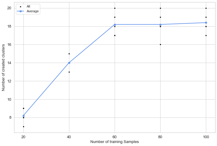
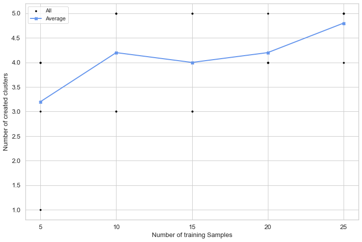
When randomly drawing training samples from the corpus, we may fail to draw one document from each class. This is done to simulate real-world applications. While the accuracy of the model can subsequently suffer from that, the model still creates coherent topics. However, for the 20 Newsgroups dataset, the model created less than the actual 20 prevalent topics from the dataset. Figure 2 show the dependency of the number of randomly drawn documents and created topics. As the dataset contains multiple topics that are very similar to one another, the number of extracted topics is still reasonable, which is also represented by the good coherence scores.

Figure 2: Average number of extracted topics per labeled training samples for the 20 Newsgroups dataset. This is only for the completely randomly drawn labels. With a larger number of extracted training samples, the model is closer to the true number of classes present in the dataset.

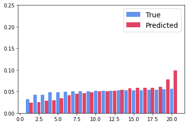
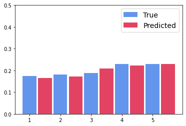
To control for the model not creating arbitrarily large garbage topics and creating bad document-topic distributions, we check the created argmax predicion distribution against the true document topic distribution, see Figure 3. We find that although the model over and underestimates mainly 4 topics, the overall distribution does not suggest the creation of large garbage topics.

Figure 3: Predicted topic distribution vs. true topic distribution. Results are achieved with DCTE on two labeled samples per class. Given the similarity of topics like mac.hardwarde and pc.hardware or religion.christian and religion.misc the achieved distribution, in combination with the achieved accuracies is reasonable.

BBC News

For the BBC News dataset, most benchmark models struggle to identify the underlying latent topics. This is presumably due to the small amount of training data. As DCTE uses little training data anyway, the number of samples in a corpus does not effect the model’s results. Table 5 shows two exemplary topics from DCTE using one labeled training sample per class. The topics entertainment and education are clearly distinguishable.

Topic	Entertainment	Education
	film	school
	actor	education
	award	child
	actress	teacher
	star	pupil
	aviator	student
	director	sport
	role	university
	nomination	parent
	oscar	democracy
NPMI	0.46	0.22

Table 5: Topics created with DCTE and the respective NPMI coherence scores for the BBC News dataset. The topics Entertainment and Education are clearly assignable.

When randomly drawing training samples from the corpus, it might happen that we fail to draw one document from each class. This leads to the model detecting as many topics as we have classes in our training data. However, only labeling 25 documents already leads to 4.8 detected topics on average over 5 runs. As unsupervised methods require setting a fixed number of topics in advance, we believe that this is not a significant drawback of the model.

Figure 4: Average number of extracted topics per labeled training samples. This is only for the completely randomly drawn labels.

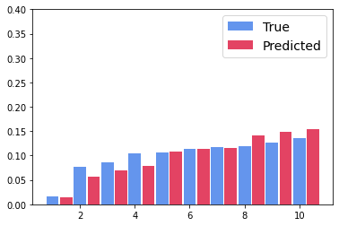
We again analyze the document-topic distributions. For the BBC News dataset all document classes are nearly equally present in the dataset, which is also captured by the presented method.

Figure 5: Predicted topic distribution vs. true topic distribution. Results are achieved with DCTE on two labeled samples per class. Randomly drawing 10 samples from the dataset already leads to averagely more than 4 extracted topics.

M10

While the achieved coherence scores for the M10 dataset are not as good as for the other datasets, the created topics are still fairly well interpretable. Table 6 shows two topics created with the presented method and their respective coherence scores. The two topics, agriculture and financial economics present in the M10 corpus are clearly identifiable.

Topic	Agriculture	Financial Economics
	crop	market
	water	stock
	soil	price
	yield	rate
	climate	volatility
	change	option
	irrigation	return
	management	pricing
	area	risk
	plant	exchange
NPMI	0.155	0.191

Table 6: Topics created with DCTE and the respective NPMI coherence scores for the M10 dataset. The topics Agriculture and Financial Economics are accurately represented.

When randomly drawing training samples from the corpus, it might happen that we fail to draw one document from each class. This leads to the model detecting as any topics as we have classes in our training data. However, only labeling 40 documents already leads to 8.8 detected topics on average over 5 runs.

Figure 6: Average number of extracted topics per labeled training samples. This is only for the completely randomly drawn labels.

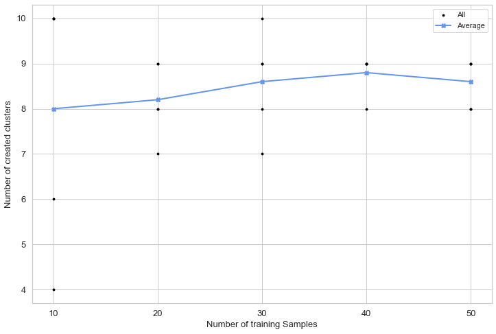
For the M10 dataset we have a slightly skewed document-topic distribution. This is also captured by the model, although the underrepresented classes are slightly more often predicted than they are truly prevalent. This could be due to the fact, that the training data does not accurately depict the true document-topic distribution prevalent in the dataset but is equally distributed over all classes.

Figure 7: Predicted topic distribution vs. true topic distribution. Results are achieved with DCTE on two labeled samples per class.

References

- Angelov (2020) Dimo Angelov. 2020. Top2vec: Distributed representations of topics. arXiv preprint arXiv:2008.09470.
- Bianchi et al. (2020) Federico Bianchi, Silvia Terragni, and Dirk Hovy. 2020. Pre-training is a hot topic: Contextualized document embeddings improve topic coherence. arXiv preprint arXiv:2004.03974.
- Bianchi et al. (2021) Federico Bianchi, Silvia Terragni, Dirk Hovy, Debora Nozza, and Elisabetta Fersini. 2021. Cross-lingual contextualized topic models with zero-shot learning. In Proceedings of the 16th Conference of the European Chapter of the Association for Computational Linguistics: Main Volume, pages 1676–1683, Online. Association for Computational Linguistics.
- Blei et al. (2003) David M Blei, Andrew Y Ng, and Michael I Jordan. 2003. Latent dirichlet allocation. Journal of machine Learning research, 3(Jan):993–1022.
- Boyd-Graber et al. (2017) Jordan Boyd-Graber, Yuening Hu, David Mimno, et al. 2017. Applications of topic models. Foundations and Trends® in Information Retrieval, 11(2-3):143–296.
- Cao et al. (2020) Kaidi Cao, Maria Brbic, and Jure Leskovec. 2020. Concept learners for few-shot learning. arXiv preprint arXiv:2007.07375.
- Chien et al. (2018) Jen-Tzung Chien, Chao-Hsi Lee, and Zheng-Hua Tan. 2018. Latent dirichlet mixture model. Neurocomputing, 278:12–22.
- Daud et al. (2010) Ali Daud, Juanzi Li, Lizhu Zhou, and Faqir Muhammad. 2010. Knowledge discovery through directed probabilistic topic models: a survey. Frontiers of computer science in China, 4(2):280–301.
- Devlin et al. (2018) Jacob Devlin, Ming-Wei Chang, Kenton Lee, and Kristina Toutanova. 2018. Bert: Pre-training of deep bidirectional transformers for language understanding. arXiv preprint arXiv:1810.04805.
- Dieng et al. (2020) Adji B Dieng, Francisco JR Ruiz, and David M Blei. 2020. Topic modeling in embedding spaces. Transactions of the Association for Computational Linguistics, 8:439–453.
- Duan et al. (2022) Zhibin Duan, Yishi Xu, Jianqiao Sun, Bo Chen, Wenchao Chen, Chaojie Wang, and Mingyuan Zhou. 2022. Bayesian deep embedding topic meta-learner. In International Conference on Machine Learning, pages 5659–5670. PMLR.
- Granić and Marangunić (2019) Andrina Granić and Nikola Marangunić. 2019. Technology acceptance model in educational context: A systematic literature review. British Journal of Educational Technology, 50(5):2572–2593.
- Grootendorst (2022) Maarten Grootendorst. 2022. Bertopic: Neural topic modeling with a class-based tf-idf procedure. arXiv preprint arXiv:2203.05794.
- Hall et al. (2008) David Hall, Dan Jurafsky, and Christopher D Manning. 2008. Studying the history of ideas using topic models. In Proceedings of the 2008 conference on empirical methods in natural language processing, pages 363–371.
- Hannigan et al. (2019) Timothy R Hannigan, Richard FJ Haans, Keyvan Vakili, Hovig Tchalian, Vern L Glaser, Milo Shaoqing Wang, Sarah Kaplan, and P Devereaux Jennings. 2019. Topic modeling in management research: Rendering new theory from textual data. Academy of Management Annals, 13(2):586–632.
- Iwata (2021) Tomoharu Iwata. 2021. Few-shot learning for topic modeling. arXiv preprint arXiv:2104.09011.
- Jelodar et al. (2019) Hamed Jelodar, Yongli Wang, Chi Yuan, Xia Feng, Xiahui Jiang, Yanchao Li, and Liang Zhao. 2019. Latent dirichlet allocation (lda) and topic modeling: models, applications, a survey. Multimedia Tools and Applications, 78(11):15169–15211.
- Larochelle and Lauly (2012) Hugo Larochelle and Stanislas Lauly. 2012. A neural autoregressive topic model. Advances in Neural Information Processing Systems, 25.
- Lau et al. (2014) Jey Han Lau, David Newman, and Timothy Baldwin. 2014. Machine reading tea leaves: Automatically evaluating topic coherence and topic model quality. In Proceedings of the 14th Conference of the European Chapter of the Association for Computational Linguistics, pages 530–539.
- Le and Mikolov (2014) Quoc Le and Tomas Mikolov. 2014. Distributed representations of sentences and documents. In International conference on machine learning, pages 1188–1196. PMLR.
- Liu et al. (2019a) Guiwen Liu, Juma Hamisi Nzige, and Kaijian Li. 2019a. Trending topics and themes in offsite construction (osc) research: The application of topic modelling. Construction innovation.
- Liu et al. (2016) Lin Liu, Lin Tang, Wen Dong, Shaowen Yao, and Wei Zhou. 2016. An overview of topic modeling and its current applications in bioinformatics. SpringerPlus, 5(1):1–22.
- Liu et al. (2019b) Yinhan Liu, Myle Ott, Naman Goyal, Jingfei Du, Mandar Joshi, Danqi Chen, Omer Levy, Mike Lewis, Luke Zettlemoyer, and Veselin Stoyanov. 2019b. Roberta: A robustly optimized bert pretraining approach. arXiv preprint arXiv:1907.11692.
- Maier et al. (2018) Daniel Maier, Annie Waldherr, Peter Miltner, Gregor Wiedemann, Andreas Niekler, Alexa Keinert, Barbara Pfetsch, Gerhard Heyer, Ueli Reber, Thomas Häussler, et al. 2018. Applying lda topic modeling in communication research: Toward a valid and reliable methodology. Communication Methods and Measures, 12(2-3):93–118.
- McInnes et al. (2017) Leland McInnes, John Healy, and Steve Astels. 2017. hdbscan: Hierarchical density based clustering. J. Open Source Softw., 2(11):205.
- McInnes et al. (2018) Leland McInnes, John Healy, and James Melville. 2018. Umap: Uniform manifold approximation and projection for dimension reduction. arXiv preprint arXiv:1802.03426.
- Mikolov et al. (2013) Tomas Mikolov, Kai Chen, Greg Corrado, and Jeffrey Dean. 2013. Efficient estimation of word representations in vector space. arXiv preprint arXiv:1301.3781.
- Pan et al. (2019) Chongyu Pan, Jian Huang, Jianxing Gong, and Xingsheng Yuan. 2019. Few-shot transfer learning for text classification with lightweight word embedding based models. IEEE Access, 7:53296–53304.
- Ramage et al. (2009) Daniel Ramage, David Hall, Ramesh Nallapati, and Christopher D Manning. 2009. Labeled lda: A supervised topic model for credit attribution in multi-labeled corpora. In Proceedings of the 2009 conference on empirical methods in natural language processing, pages 248–256.
- Ramage et al. (2011) Daniel Ramage, Christopher D Manning, and Susan Dumais. 2011. Partially labeled topic models for interpretable text mining. In Proceedings of the 17th ACM SIGKDD international conference on Knowledge discovery and data mining, pages 457–465.
- Reimers and Gurevych (2019) Nils Reimers and Iryna Gurevych. 2019. Sentence-bert: Sentence embeddings using siamese bert-networks. In Proceedings of the 2019 Conference on Empirical Methods in Natural Language Processing. Association for Computational Linguistics.
- Reimers and Gurevych (2020) Nils Reimers and Iryna Gurevych. 2020. Making monolingual sentence embeddings multilingual using knowledge distillation. In Proceedings of the 2020 Conference on Empirical Methods in Natural Language Processing. Association for Computational Linguistics.
- Reynolds (2009) Douglas A Reynolds. 2009. Gaussian mixture models. Encyclopedia of biometrics, 741(659-663).
- Rios and Kavuluru (2018) Anthony Rios and Ramakanth Kavuluru. 2018. Few-shot and zero-shot multi-label learning for structured label spaces. In Proceedings of the Conference on Empirical Methods in Natural Language Processing. Conference on Empirical Methods in Natural Language Processing, volume 2018, page 3132. NIH Public Access.
- Salton (1989) Gerard Salton. 1989. Automatic text processing: The transformation, analysis, and retrieval of. Reading: Addison-Wesley, 169.
- Sia et al. (2020) Suzanna Sia, Ayush Dalmia, and Sabrina J Mielke. 2020. Tired of topic models? clusters of pretrained word embeddings make for fast and good topics too! arXiv preprint arXiv:2004.14914.
- Srivastava and Sutton (2017) Akash Srivastava and Charles Sutton. 2017. Autoencoding variational inference for topic models. arXiv preprint arXiv:1703.01488.
- Terragni et al. (2021) Silvia Terragni, Elisabetta Fersini, Bruno Giovanni Galuzzi, Pietro Tropeano, and Antonio Candelieri. 2021. Octis: Comparing and optimizing topic models is simple! In Proceedings of the 16th Conference of the European Chapter of the Association for Computational Linguistics: System Demonstrations, pages 263–270.
- Tunstall et al. (2022) Lewis Tunstall, Nils Reimers, Unso Eun Seo Jo, Luke Bates, Daniel Korat, Moshe Wasserblat, and Oren Pereg. 2022. Efficient few-shot learning without prompts. arXiv preprint arXiv:2209.11055.
- Wang et al. (2019) Rui Wang, Deyu Zhou, and Yulan He. 2019. Atm: Adversarial-neural topic model. Information Processing & Management, 56(6):102098.