Difformer: Empowering Diffusion Models on the Embedding Space
for Text Generation

Abstract

Diffusion models have achieved state-of-the-art synthesis quality on both visual and audio tasks, and recent works further adapt them to textual data by diffusing on the embedding space. In this paper, we conduct systematic studies and analyze the challenges between the continuous data space and the embedding space which have not been carefully explored. Firstly, the data distribution is learnable for embeddings, which may lead to the collapse of the loss function. Secondly, as the norm of embeddings varies between popular and rare words, adding the same noise scale will lead to sub-optimal results. In addition, we find the normal level of noise causes insufficient training of the model. To address the above challenges, we propose Difformer, an embedding diffusion model based on Transformer, which consists of three essential modules including an additional anchor loss function, a layer normalization module for embeddings, and a noise factor to the Gaussian noise. Experiments on two seminal text generation tasks including machine translation and text summarization show the superiority of Difformer over compared embedding diffusion baselines.

1 Introduction

A wave of diffusion models (Sohl-Dickstein et al., 2015; Ho et al., 2020) is sweeping the generation tasks (e.g., image and audio synthesis) recently, showing their great potential for high-quality data generation. Diffusion models are a family of iterative generative models, which are trained to recover corrupted data and then generate data by gradually refining samples from the pure noise. This procedure enables the model to make subtle refinements of output samples in a multi-step denoising process, and thus generate high-fidelity samples (Rombach et al., 2022; Chen et al., 2020).

Besides the booming achievements on vision (Song et al., 2020; Dhariwal & Nichol, 2021; Nichol & Dhariwal, 2021; Ho & Salimans, 2021; Rombach et al., 2022) and audio (Chen et al., 2020; Kong et al., 2020) generation, the exploration of diffusion models on text generation is still at an initial stage. Recent works (Li et al., 2022; Gong et al., 2022; Strudel et al., 2022) basically convert the discrete tokens to embeddings and then utilize continuous diffusion models to generate them, which can be termed embedding diffusion models. These preliminary attempts follow the original model to deal with the embeddings, with little consideration of the unique properties of the embedding data space which is learned from scratch.

In this paper, we conduct a thorough study of the challenges of embedding diffusion models, which are divided into three-fold. Firstly, for diffusion models on image and audio generation, the ground truth data, i.e., the initial state of the forward diffusion process, is fixed during training. In contrast, it is learnable for textual data (i.e., embeddings), which may cause the collapse of the embeddings space and bring instability to the training of the model. We analyze this problem in Section 3.1. Secondly, the long-tailed problem occurs widely in natural language processing (Schakel & Wilson, 2015), i.e., the imbalanced frequency of popular and rare words makes their learned embeddings diverge, which is discussed in Section 3.2. As a result, the embedding scales of different words are diverse, and it would be sub-optimal to add the same scale of noise to embeddings of different words. Thirdly, in Section 3.3, we find the normal noise provides relatively simple denoising objectives at most of the forward steps, which causes the insufficient training of the model.

To tackle the above challenges, in this paper, we propose Difformer, a denoising diffusion Transformer model. Specifically, to avoid the collapse of the denoising loss function with moving embedding parameters, we propose an anchor loss function to stabilize the training process. Then, we introduce a layer normalization module on the top of the embedding layer to regularize the embeddings of popular and rare words into a uniform scale, eliminating the effect of varied scales on them. In addition, we increase the scale of the added Gaussian noise by introducing a hyper-parameter named the noise factor, to enhance the guidance provided by the denoising objective at each diffusion step. We conduct experiments on two important text generation tasks including machine translation and text summarization. On all five benchmark datasets, Difformer largely outperforms diffusion-based and iteration-based non-autoregressive baselines.

Our contributions can be summarized as follows:

• We conduct thorough studies on several key problems when applying continuous diffusion models to discrete text generation tasks, including the collapse of the denoising objective, the imbalanced embedding scales over words, and the insufficient training caused by inadequate noise.

• We propose Difformer, a continuous diffusion model that solves the problems with three key components, i.e., an anchor loss function, a layer normalization module over the embeddings, and a noise factor that enlarges the scale of the added noise.

• We evaluate the performance of Difformer on machine translation and text summarization tasks, which consistently achieves better results compared with diffusion-based models.

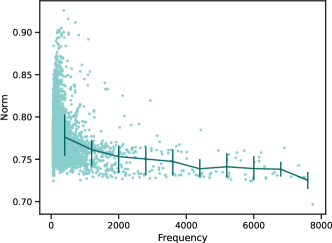
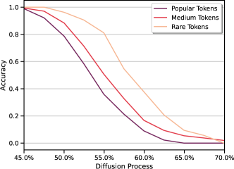
Figure 1: (a) Distribution of the embedding norm over the token frequency. Embeddings of tokens with lower frequency tend to have larger norms, while those with higher frequency have smaller norms. (b) The classification accuracy based on whether the nearest neighbor of the noisy embedding $\mathbb{z}_{t}$ is still $\mathbb{z}_{0}$ at different diffusion steps $t$. Different curves correspond to embeddings with different token frequencies.

2 Background

Diffusion Models

Denoising diffusion probabilistic models (Sohl-Dickstein et al., 2015; Ho et al., 2020) utilize a forward process to perturb the data with Gaussian noise step by step, and a reverse process to restore the data symmetrically. Ho et al. (2020) develop the approach by specific parameterizations and achieve the comparable sample quality with state-of-the-art generative models such as GANs (Goodfellow Ian et al., 2014). After that, great improvements have been made by many following works (Song et al., 2020; Dhariwal & Nichol, 2021; Nichol & Dhariwal, 2021; Rombach et al., 2022) both in quality and efficiency.

Specifically, given a data sample $\mathbb{z}_{0}\in\mathbb{R}^{d}$, the denoising diffusion probabilistic model (Ho et al., 2020) gradually perturbs it into a pure Gaussian noise $\mathbb{z}_{T}\sim\mathcal{N}(\mathbf{0},\mathbf{I})$ through a series of latent variables $\mathbb{z}_{1},\cdots,\mathbb{z}_{T}$ in the forward process, and each step is a Markov transition:

$$q(\mathbb{z}_{t}|\mathbb{z}_{t-1})=\mathcal{N}(\mathbb{z}_{t};\sqrt{1-\beta_{t}}\mathbb{z}_{t-1},\beta_{t}\mathbf{I}),$$ (1)

where $\beta_{t}$ controls the noise level added at timestep $t$, and for any arbitrary $t$, sampling $\mathbb{z}_{t}$ from $\mathbb{z}_{0}$ can be achieved in a closed form:

$$q(\mathbb{z}_{t}|\mathbb{z}_{0})=\mathcal{N}(\mathbb{z}_{t};\sqrt{1-\bar{\beta}_{t}}\mathbb{z}_{0},\bar{\beta}_{t}\mathbf{I}),$$ (2)

where $\bar{\beta}_{t}:=1-\prod_{i=0}^{t}(1-\beta_{i})$. In the reverse process, the model recovers the data $\mathbb{z}_{0}$ by denoising from $\mathbb{z}_{T}$ with each step parameterized as:

$$p_{\theta}(\mathbb{z}_{t-1}|\mathbb{z}_{t})=\mathcal{N}(\mathbb{z}_{t-1};\boldsymbol{\mu}_{\theta}(\mathbb{z}_{t},t),\boldsymbol{\Sigma}_{\theta}(\mathbb{z}_{t},t)),$$ (3)

where $\boldsymbol{\mu}_{\theta}(\cdot)$ and $\boldsymbol{\Sigma}_{\theta}(\cdot)$ are the predicted mean and covariance of $q(\mathbb{z}_{t-1}|\mathbb{z}_{t})$, and $\theta$ denotes the model parameters. Following the derivation in Ho et al. (2020), we set $\boldsymbol{\Sigma}_{\theta}(\mathbb{z}_{t},t)=\sigma_{t}^{2}\mathbf{I}$. The objective function of the diffusion model is the variational lower-bound (VLB) of $\log p_{\theta}(\mathbb{z}_{0})$, which can be written as:

$$\mathcal{L}_{\mathrm{vlb}}=\mathbb{E}_{\mathbb{z}_{0},t}\left[\frac{1}{2\sigma_{t}^{2}}\left\lVert\tilde{\boldsymbol{\mu}}_{t}(\mathbb{z}_{t},\mathbb{z}_{0})-\boldsymbol{\mu}_{\theta}(\mathbb{z}_{t},t)\right\rVert^{2}\right],$$

where $\tilde{\boldsymbol{\mu}}_{t}$ denotes the mean of $q(\mathbb{z}_{t-1}|\mathbb{z}_{t},\mathbb{z}_{0})$. We further parameterize $\boldsymbol{\mu}_{\theta}(\mathbb{z}_{t},t):=\tilde{\boldsymbol{\mu}}_{t}(\mathbb{z}_{t},\hat{\mathbb{z}}_{0})$, where $\hat{\mathbb{z}}_{0}$ is the model prediction of the golden data $\mathbb{z}_{0}$, i.e., $\hat{\mathbb{z}}_{0}:=f_{\theta}(\mathbb{z}_{t},t)$, and $f_{\theta}(\cdot)$ represents the neural network. Then we could simplify the objective function as:

$$\mathcal{L}_{\mathrm{vlb}}=\mathbb{E}_{\mathbb{z}_{0},t}\left[\left\lVert\hat{\mathbb{z}}_{0}-\mathbb{z}_{0}\right\rVert^{2}\right].$$ (4)

Diffusion Models on Text Generation

The breakthrough of diffusion models on continuous data encourages people to explore their capacity on discrete textual data. Recent works mainly follow two directions. Firstly, discrete diffusion models (Hoogeboom et al., 2021; Austin et al., 2021b; Savinov et al., 2021; Reid et al., 2022) that build on categorical distributions are proposed, in which sentences are corrupted and refined in the token level. Attempts have also been made to expolore modeling on surrogate representations of discrete data such as analog bits (Chen et al., 2022) and simplex (Han et al., 2022). However, these kinds of corruptions are coarse-grained and not able to model the semantic correlations between tokens.

In contrast, to deal with diffusion on discrete data, recent works (Li et al., 2022; Strudel et al., 2022; Gong et al., 2022) propose additional embedding and rounding steps in the forward and reverse processes respectively to convert tokens into embeddings, and then utilize continuous diffusion models to add Gaussian noise controlled by a smooth schedule function to embeddings, achieving a fine-grained sampling procedure. Specifically, given a sequence of tokens $\boldsymbol{y}$, the embedding step can be denoted as $\mathbb{z}_{0}\sim\mathcal{N}(\boldsymbol{e}(\boldsymbol{y}),\beta_{0}\mathbf{I})$ where $\boldsymbol{e}(\cdot)$ denotes the embedding lookup function, and the rounding step as $p_{\theta}(\boldsymbol{y}|\mathbb{z}_{0})$, i.e., a softmax distribution over the vocabulary, with an extra loss function $\mathcal{L}_{\mathrm{round}}=-\log p_{\theta}(\boldsymbol{y}|\mathbb{z}_{0})$ which is added to Equ (4). Nevertheless, these works directly adapt continuous diffusion models to embeddings, without considering the differences between the learnable embedding space and fixed image or audio data, as well as the unique properties of embeddings learned from the discrete textual corpus. Furthermore, there is still a lack of comprehensive analysis of the challenges of embedding diffusion models, especially on benchmark text generation tasks such as machine translation and text summarization.

3 Challenges of Diffusion Models on Embeddings

We start with analyzing the challenges of applying continuous diffusion models on the embedding space with empirical investigations in this section. Specifically, we train diffusion models on the IWSLT14 German to English machine translation task, which is a widely used benchmark dataset. The model architecture is based on Transformer (Vaswani et al., 2017). Given a source sentence $\boldsymbol{x}=[x_{1},x_{2},\cdots,x_{m}]$, the encoder outputs its hidden representation, which is taken as the condition of the decoder to generate the target sentence $\boldsymbol{y}=[y_{1},y_{2},\cdots,y_{n}]$. The loss function is equivalent to Equ (4) with conditioning on $\boldsymbol{x}$, where the model prediction is $\hat{\mathbb{z}}_{0}=f_{\theta}(\mathbb{z}_{t},t;\boldsymbol{x})$.

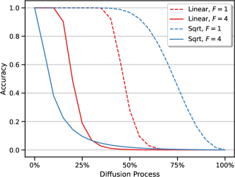
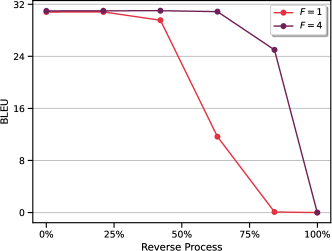
Figure 2: (a) The classification accuracy with different noise schedules and noise factors. $F$ is the noise factor introduced in Section 4.3, and $F=1$ indicates the original model. (b) BLEU scores of models fed with pure Gaussian noise $\mathbb{z}_{T}$ rather than $\mathbb{z}_{t}$.

3.1 Collapse of the Denoising Objective

The data space is usually fixed for continuous data (e.g., image and audio), but is learned from scratch for discrete textual data (i.e., embeddings), which is therefore dynamic during training. Original diffusion models rely on the loss function in Equ (4) to learn the noise added to the data sample $\mathbb{z}_{0}$. But the loss will collapse when jointly training both the model parameters and embeddings, because the model can easily reach a trivial solution that all embeddings are similar to each other and located in a small sub-region of the embedding space, which can be termed as anisotropic embeddings (Ethayarajh, 2019). Formally, we can measure the anisotropy of embeddings by computing the self-similarity score:

$$\mathrm{ANI}=\frac{1}{C}\sum_{i=1}^{|V|}\sum_{j=1,j\neq i}^{|V|}\cos(\boldsymbol{e}(i),\boldsymbol{e}(j)),$$ (5)

where $|V|$ is the vocabulary size, and $C=|V|\times(|V|-1)$ indicates the total number of embedding pairs. Essentially, the lower the anisotropy is, the better the embeddings are. Because with higher anisotropy scores, the embeddings of different tokens are less discriminative and non-uniformly distributed in the space, and thus limit the representation quality of the model. As a result, with only $\mathcal{L}_{\mathrm{vlb}}$, the anisotropy score is as high as $0.99$, indicating that the embeddings are collapsed.

Recent works of diffusion model on embeddings (Li et al., 2022; Gong et al., 2022) introduce the rounding loss $\mathcal{L}_{\mathrm{round}}$ to alleviate this problem, which we find is not sufficient to provide strong constraints. In experiments, we observe that the rounding loss descends drastically and falls to near zero in the first several steps. In addition, the anisotropy score of the learned embeddings is $0.32$, which is still very high. The reason is that although $\mathcal{L}_{\mathrm{round}}=-\log p_{\theta}(\boldsymbol{y}|\mathbb{z}_{0})$ is based on the cross-entropy that can push different embeddings apart, it is limited considering that the input $\mathbb{z}_{0}$ is obtained from the original embedding $\boldsymbol{e}(\boldsymbol{y})$ with a small amount of noise added. We have also tried increasing the weight of $\mathcal{L}_{\mathrm{round}}$ or the scale of the added noise, both of which do not solve the problem though. Correspondingly, in experiments, we find that the performance of $\mathcal{L}_{\mathrm{round}}$ is sup-optimal, which also requires careful tuning of hyper-parameters to make use of the rounding loss.

3.2 Imbalanced Embedding Scale

As discussed earlier, due to the imbalanced frequency of tokens in natural language processing datasets, the token embeddings will also have different frequencies to the loss function as well as gradients, which will finally lead to different scales (i.e., $L_{2}$ norms) of the learned embeddings. In Figure 1, we show the joint distribution of the frequency of a token and its embedding norm from a well-trained Transformer (Vaswani et al., 2017). We find that there exists a negative correlation between the embedding norm and frequency of tokens, which indicates that the embeddings of rare tokens are more likely to have large norms, as supported in previous works (Schakel & Wilson, 2015; Liu et al., 2020).

Based on this fact, it will be sub-optimal to add the same amount of noise to different embeddings, as embeddings with larger norms require more noise to wipe out their intrinsic information, while it is the opposite for embeddings with smaller norms. As shown in Figure 1, when adding noises to tokens with different frequencies, embeddings of rare tokens require more steps to distinguish from their noisy counterparts due to the large values of norms, while frequent tokens need less correspondingly.

3.3 Insufficient Training of the Model

The design of the noise schedule, which determines the amount of noise added to the data at each step, has significant influences on both forward and reverse processes. Intuitively, during training, denoising is a more challenging task for the model at steps with higher noise levels, which becomes trivial when the noise level is too low. Too many steps with low noise levels will make the training insufficient. Several widely utilized noise schedules have been proposed by previous works, such as linear (Ho et al., 2020) and sqrt (Li et al., 2022). We analyze the effectiveness of these schedules on the embedding space in Figure 2. Specifically, to evaluate the difficulty of recovering from noised embeddings, we compute the accuracy of classifying them to the original tokens with the nearest neighbor classifier.

As illustrated in Figure 2 where $F=1$ indicates the original model, a simple classifier is able to achieve high accuracy when predicting tokens from noised embeddings at most of the diffusion steps. In other words, $\mathbb{z}_{t}$ remains in the nearest neighbor region of $\boldsymbol{e}(\boldsymbol{y})$ even after adding a large amount of noise. Consequently, the model is dealing with simple denoising tasks and thus not well optimized most of the time, which hampers the model performance in the reverse process. In Figure 2, we evaluate the denoising capability of the model by taking $\mathbb{z}_{T}$ as input at different diffusion steps $t$, and compute the BLEU score of the output $\hat{\mathbb{z}}_{0}$ at each step, i.e., the model recovers $\hat{\mathbb{z}}_{0}$ from pure noise only with the condition from the source side, and higher BLEU scores indicate better denoising capacity. We can notice that the BLEU score drops dramatically at steps with low-level noises, i.e., the model training on these steps is insufficient.

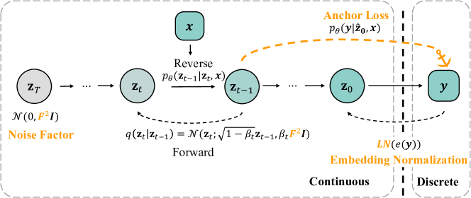
Figure 3: An overview of the proposed Difformer, including the three main contributions, i.e., the anchor loss function, the embedding normalization, and the noise factor.

4 Difformer: Denoising Diffusion based on Transformer

After analyzing the challenges of continuous diffusion models on embeddings, in this section, we proceed to introduce Difformer, a denoising diffusion model with Transformer, to tackle the challenges correspondingly. We provide an overview of the model in Figure 3.

4.1 The Anchor Loss Function

A straightforward solution to the first challenge is to replace the randomly initialized embedding matrix with a pre-trained one (e.g., embeddings from pre-trained language models such as BERT (Devlin et al., 2019)) and fix it during training. However, considering the variety of loss functions and tasks, simply fixing the pre-trained embeddings is sub-optimal for diffusion models (Gong et al., 2022).

Different from simply employing the embeddings from pre-trained models, we propose a training objective named the anchor loss:

$$\mathcal{L}_{\mathrm{anchor}}=-\log p_{\theta}(\boldsymbol{y}|\hat{\mathbb{z}}_{0}).$$ (6)

Comparing with $\mathcal{L}_{\mathrm{round}}$, $\mathcal{L}_{\mathrm{anchor}}$ utilizes prediction $\hat{\mathbb{z}}_{0}$ as the input instead of the golden embedding $\mathbb{z}_{0}$. Intuitively, while both loss functions aim at pushing embeddings apart to prevent the collapse of the denoising objectives, $\mathcal{L}_{\mathrm{round}}$ uses the noisy embedding $\mathbb{z}_{0}\sim\mathcal{N}(\boldsymbol{e}(\boldsymbol{y}),\beta_{0}\mathbf{I})$ to predict the embedding $\boldsymbol{e}(\boldsymbol{y})$, where the distance between $\mathbb{z}_{0}$ and $\boldsymbol{e}(\boldsymbol{y})$ can be too small to provide useful guidance as analyzed in Section 3.1. In contrast, for $\mathcal{L}_{\mathrm{anchor}}$, by using the model output $\hat{\mathbb{z}}_{0}$ which contains the prediction errors of the model, the loss function jointly optimizes the embeddings and model parameters, i.e., the gradients of embeddings are back-propagated from model parameters, and therefore successfully provides regularizations to the embeddings. As a result, the anisotropic score of the embeddings learned by optimizing $\mathcal{L}_{\mathrm{anchor}}$ is as low as $0.03$, indicating that the embeddings are informative and discriminative to each other.

4.2 Layer Normalization on Embeddings

To deal with the imbalanced embedding scales, we introduce a layer normalization module on the top of the embedding layer to ensure the uniform scale of tokens. Specifically, for the embedding $\boldsymbol{e}(y_{i})$ of token $y_{i}$, the module re-scales its distribution by:

$$\mathrm{LN}(\boldsymbol{e}(y_{i}))=\frac{\boldsymbol{e}(y_{i})-\mathbb{E}[\boldsymbol{e}(y_{i})]}{\sqrt{\mathbb{V}[\boldsymbol{e}(y_{i})]+\epsilon}}\odot\boldsymbol{\gamma}+\boldsymbol{\eta},$$

where $\odot$ denotes element-wise multiplication, $\mathbb{E}[\cdot]$ and $\mathbb{V}[\cdot]$ indicate the expectation and variance respectively, $\boldsymbol{\gamma}$ and $\boldsymbol{\eta}$ are learnable parameters and $\epsilon$ is a small number to prevent overflow.

Consequentially, as the parameters $\boldsymbol{\gamma}$ and $\boldsymbol{\eta}$ are shared across all embeddings, embeddings of different tokens will be normalized to the same scale, which eliminates the imbalanced scale problem illustrated in Section 3.2.

4.3 The Noise Factor

To alleviate the insufficient training brought by standard Gaussian noise, we propose a simple but effective method by manually magnifying the scale of noise added at each step. Concretely, we generalize the covariance matrix of $q(\mathbb{z}_{t}|\mathbb{z}_{t-1})$ from $\beta_{t}\mathbf{I}$ to $\beta_{t}F^{2}\mathbf{I}$, where $F$ is a hyper-parameter termed as the noise factor. Formally, each forward step in Equ (1) can be written as:

$$q(\mathbb{z}_{t}|\mathbb{z}_{t-1})=\mathcal{N}(\mathbb{z}_{t};\sqrt{1-\beta_{t}}\mathbb{z}_{t-1},\beta_{t}F^{2}\mathbf{I}).$$ (7)

Correspondingly, the prior becomes $p(\mathbb{z}_{T})=\mathcal{N}(\mathbb{z}_{T};\mathbf{0},F^{2}\mathbf{I})$, where $F=1$ is equivalent to the original prior.

In this way, the difference between $\mathbb{z}_{t}$ and $\boldsymbol{e}(\boldsymbol{y})$ is enlarged. As shown in Figure 2, after multiplying by the noise factor, the nearest neighbor classification accuracy drops at much earlier steps which ensures the model can be well optimized by the denoising objective at most diffusion steps. We can regard this modification as a kind of data augmentation because it enables the model to be trained on harder samples than the original one, thus enhancing the generalization capability of the model significantly at steps with small noise, which can be illustrated in Figure 2, where the model with the noise factor performs better at smaller steps in the reverse process.

It is worth noting that noise factor and noise schedule are two orthogonal techniques that control the level of noise, which are complementary to each other. Our experimental results show that the noise factor achieves improvements over all considered noise schedules.

4.4 Training and Inference

Training objective

Given a source sentence $\boldsymbol{x}=[x_{1},x_{2},\cdots,x_{m}]$, the model learns to generate the target sentence $\boldsymbol{y}=[y_{1},y_{2},\cdots,y_{n}]$ by estimating $p_{\theta}(\boldsymbol{y}|\boldsymbol{x})$. Traditional models (Vaswani et al., 2017) factorize the distribution in an autoregressive way and estimate tokens with left-to-right sequential conditions, i.e., $p_{\theta}(\boldsymbol{y}|\boldsymbol{x})=\prod_{i=1}^{n}p_{\theta}(y_{i}|\boldsymbol{y}_{<i},\boldsymbol{x})$. In comparison, diffusion models (Gong et al., 2022; Strudel et al., 2022) break the conditional dependency between tokens and estimate all tokens simultaneously in a non-autoregressive way (Gu et al., 2018), i.e., $p_{\theta}(\boldsymbol{y}|\boldsymbol{x})=\prod_{i=1}^{n}p_{\theta}(y_{i}|\mathbb{z},\boldsymbol{x})$. In this framework, the final objective function of our model can be written as:

$$\mathcal{L}=\mathbb{E}_{(\boldsymbol{x},\boldsymbol{y}),\mathbb{z}_{0},t}\left[\lVert\hat{\mathbb{z}}_{0}-\mathbb{z}_{0}\rVert^{2}-\log p_{\theta}(\boldsymbol{y}|\hat{\mathbb{z}}_{0})\right],$$ (8)

where the first and second items refer to $\mathcal{L}_{\mathrm{vlb}}$ and $\mathcal{L}_{\mathrm{anchor}}$ respectively.

Length Prediction and 2D Parallel Decoding

Unlike traditional autoregressive models where the sequence length is implicitly modeled by the generation of the EOS token, diffusion models generate all tokens in a non-autoregressive manner, where the length should be modeled explicitly. Previous works (Li et al., 2022; Gong et al., 2022; Strudel et al., 2022) usually generate a sequence with maximum length and cutoff the content after the EOS token. In this paper, we utilize a more efficient way by explicitly predicting the target length with the encoder output (Lee et al., 2018), i.e., $p_{\theta}(n|\boldsymbol{x})$, and the negative log-likelihood loss function is added to Equ (8) while training.

A unique benefit of this approach is that we can conduct 2D parallel decoding in inference. Firstly, we can consider top-$b_{1}$ lengths from the length predictor to generate candidates with different lengths. Secondly, for each length, we can also generate $b_{2}$ candidates by sampling different initial noises from the prior. The final prediction is selected from the total $b=b_{1}\times b_{2}$ candidates that minimizes the expected risk (Kumar & Byrne, 2004) w.r.t. a metric such as BLEU or PPL. We term $b_{1}$ and $b_{2}$ as length and noise beams respectively.

Acceleration in Inference

Diffusion models are trained with thousands of forward steps, but it would be extremely time-consuming to execute all steps in inference. For Difformer, we pick a subset $\{\tau_{1},\tau_{2},\cdots,\tau_{K}\}$ of the full diffusion trajectory $\{1,2,\cdots,T\}$ for generation (Song et al., 2020; Nichol & Dhariwal, 2021). Then a reverse step can be obtained by:

$$\mathbb{z}_{\tau_{i-1}} \sim q(\mathbb{z}_{\tau_{i-1}}|\mathbb{z}_{\tau_{i}},\hat{\mathbb{z}}_{0}),$$ (9)

$$\hat{\mathbb{z}}_{0} =\hat{\mathbb{z}}_{0}(\mathbb{z}_{\tau_{i}},\tau_{i}).$$ (10)

5 Experiments

Table 1: The performance of the proposed Difformer and the baseline methods, including BLEU scores on WMT14 En-De, WMT16 En-Ro, and IWSLT14 De-En, as well as ROUGE-$1$/$2$/$L$ scores on Gigaword. ”$\Uparrow$” indicates the improvement of Difformer over the baselines with the same beam size $b$ is significant at the level of $0.01$. The baseline scores are all reported by our own implementations except CDCD.

	WMT14	WMT16	IWSLT14
Models	En$-$De	En$-$Ro	De$-$En	Gigaword
Transformer ($b=1$) (Vaswani et al., 2017)	$26.37$	$32.76$	$32.62$	$36.78$/$17.79$/$34.10$
Transformer ($b=5$)	$27.37$	$33.59$	$33.91$	$37.54$/$18.80$/$34.93$
CMLM ($b=1$) (Ghazvininejad et al., 2019)	$25.94$	$32.13$	$26.41$	$34.41$/$15.61$/$32.17$
CMLM ($b=10$)	$27.03$	$33.08$	$31.76$	$36.33$/$17.82$/$33.83$
DiffuSeq ($b=1$) (Gong et al., 2022)	$13.73$	$23.37$	$27.03$	$28.50$/$10.10$/$26.00$
DiffuSeq ($b=10$)	$15.37$	$25.45$	$28.78$	$31.17$/$12.23$/$29.24$
SeqDiffuSeq ($b=1$) (Yuan et al., 2022)	$14.37$	$23.98$	$28.65$	$30.28$/$11.72$/$28.40$
SeqDiffuSeq ($b=10$)	$17.14$	$26.17$	$30.03$	$31.90$/$12.36$/$29.22$
Difformer ($b=1$)	$26.50^{\Uparrow}$	$32.52^{\Uparrow}$	$32.18^{\Uparrow}$	$35.45$/$16.46$/$32.87^{\Uparrow}$
Difformer ($b=10$)	$27.06^{\Uparrow}$	$33.18^{\Uparrow}$	$34.05^{\Uparrow}$	${37.12}$/${18.25}$/${34.60}^{\Uparrow}$
Difformer ($b=20$)	27.23	33.36	34.13	37.64/18.75/35.01

Table 2: SacreBLEU results on the raw WMT14 En-De dataset. CDCD results are directly copied from their paper.

Models	SacreBLEU
CDCD ($b=1$) (Dieleman et al., 2022)	$19.30$
CDCD ($b=10$)	$19.70$
Difformer ($b=1$)	$22.30$
Difformer ($b=10$)	$23.10$
Difformer ($b=20$)	23.80

To evaluate the proposed Difformer model, we conduct experiments on two conditional text generation tasks including neural machine translation and text summarization.

5.1 Experimental Setup

Datasets

For machine translation, we consider three benchmark datasets including IWSLT14 German-English (IWSLT De-En), WMT14 English-German (WMT En-De), and WMT16 English-Romanian (WMT En-Ro), mainly following previous works (Gu et al., 2018; Guo et al., 2019; Ghazvininejad et al., 2019). For text summarization, we conduct experiments on Gigaword (Rush et al., 2017), a benchmark abstractive summarization dataset. In addition, following previous non-autoregressive text generation works (Gu et al., 2018, 2019; Ghazvininejad et al., 2019), we adopt sequence-level knowledge distillation (Kim & Rush, 2016) to distill the original training set to alleviate the multi-modality problem. We use the distilled training set for WMT datasets and the original ones for other datasets.

Baselines

We mainly compare our method with two recent embedding diffusion models, i.e., DiffuSeq (Gong et al., 2022) and SeqDiffuSeq (Yuan et al., 2022), both extend Diff-LM (Li et al., 2022) to the sequence-to-sequence scenario. We also include CMLM (Ghazvininejad et al., 2019), a conditional masked language model with iterative decoding, which can also be considered as a discrete diffusion model (Austin et al., 2021a). We further compare to a concurrent work CDCD (Dieleman et al., 2022) as the baseline. In addition, we report the performance of the autoregressive Transformer as the autoregressive baseline.

Implementation Details

We build our model on Transformer (Vaswani et al., 2017), and use transformer-iwslt-de-en config for the IWSLT dataset, while transformer-base for other datasets. We set diffusion step $T=2000$, noise factor $F=4$, and use an sqrt noise schedule. The training takes nearly one day on $8$ Nvidia V100 GPUs. We downsample the diffusion step to $20$ in inference, i.e., $K=20$, which is ten times faster than previous works (Li et al., 2022; Gong et al., 2022). We tokenize sentences and segment each token into subwords by Byte-Pair Encoding (Sennrich et al., 2015). In evaluation, we report the tokenized BLEU score (Papineni et al., 2002) for machine translation results, beside the SacreBLEU (Post, 2018) score when compared with CDCD. We use ROUGE score (Lin, 2004) for summarization.

5.2 Results

The main results are listed in Table 1. With a little abuse of notation, we use $b$ to represent the size of beam search for the Transformer baseline, as well as the size of parallel decoding (i.e., $b=b_{1}\times b_{2}$). We provide the ablation study on it in Appendix B.3. As can be observed from Table 1, the proposed Difformer outperforms both the diffusion-based and iteration-based baselines on all the datasets with different choices of $b$ and performs comparably with the autoregressive Transformer model. Specifically, the significant improvements of Difformer over the diffusion baselines confirm the challenges that occur to continuous diffusion models on text generation tasks and the effectiveness of the proposed solutions. Compared with CMLM, an iteration-based non-autoregressive baseline, Difformer outperforms on various datasets consistently. Moreover, benefiting from the stochastic nature of diffusion models, Difformer is able to conduct 2D parallel decoding over the length and noise beam at the same time, increasing its flexibility and potential to obtain better results. In contrast, the deterministic CMLM can only utilize different lengths, and we observe a performance drop when $b$ is larger than $10$.

Comparison with CDCD

We compare with a concurrent work CDCD (Dieleman et al., 2022) by strictly following their settings, i.e., utilizing the raw WMT14 En-De training set and evaluating by SacreBLEU. As shown in Table 2, the proposed Difformer achieves significantly better results with the same number of $b$.

5.3 Ablation Study

Table 3: The ablation study on the proposed different components. Results are conducted on the IWSLT De-En task with $b=1$.

Models	BLEU
(1): Difformer	32.18
(2): (1) w/o $\mathcal{L}_{\mathrm{anchor}}$	$15.90$
(3): (1) w/o Embedding Normalization	$31.95$
(4): (1) w/o Noise Factor	$2.85$

We study whether the proposed different components benefit the complete model in this section. The results of the ablation study are listed in Table 3. Firstly, while previous embedding diffusion works usually follow Diff-LM (Li et al., 2022) and utilize the rounding loss function, we find it does not provide satisfactory results (i.e., setting (2)) on the text generation tasks considered in this paper. This result echoes our findings in Section 3.1 that the rounding loss provides insufficient regularization to the embedding parameters. By replacing $\mathcal{L}_{\mathrm{round}}$ with $\mathcal{L}_{\mathrm{anchor}}$, the problem is largely alleviated with significant improvements on performance

Furthermore, the proposed noise factor and embedding normalization also help improve the model performance. The sqrt schedule has poor BLEU scores with the original noise, while the noise factor significantly boosts the performance.

5.4 Analyses

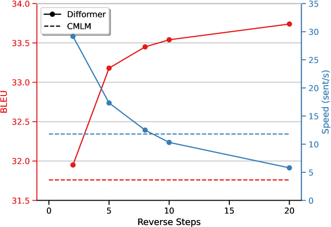
Figure 4: The results of varying the reverse step $K$. We set $b=10$ for Difformer and CMLM. The inference speed is measured by the number of generated sentences per second, and the higher the faster. Dashed lines indicate the results of the CMLM model.

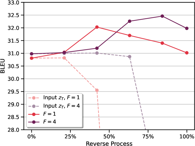
Figure 5: BLEU score of $\hat{\mathbb{z}}_{0}$ at different step. The quality of the outputs of the model increases at first and decreases later. Light-colored curves indicate the denoising capability, i.e., BLEU score of $\hat{\mathbb{z}}_{0}$ with $\mathbb{z}_{T}$ as input.

Study on the Denoising Capacity at Intermediate Steps

To evaluate the denoising capacity of the model at different diffusion steps, in the reverse process, we feed the pure noise $z_{T}$ to the decoder at each intermediate step and measure the performance of the output $\hat{\mathbb{z}}_{0}$, i.e., forcing the model to denoise only conditioned on the source representation. As illustrated by the dashed lines in Figure 5, with the original noise where $F=1$, the denoising capacity drops drastically after half of the reverse process, and the model learned with the noise factor has a stronger denoising capacity.

We then evaluate the translation performance at intermediate steps, by normally feeding $z_{t}$ to the model at step $z_{t-1}$ and measure the performance of predicted $\hat{\mathbb{z}}_{0}$. The results are illustrated as the solid lines in Figure 5. For the original noise, in the first quarter of the reverse process, the quality of $\hat{\mathbb{z}}_{0}$ continuously increases as expected, but decreases rapidly during the rest half. While setting the noise factor to $4$ alleviates this problem. Both results show that training with the noise factor prevents the model from insufficient training at low-noise steps as discussed in Section 3.3. The performance decreasing on smaller diffusion steps motivates us to propose an early stopping technique, which terminates the decoding process at an intermediate step to keep high-quality results before the performance decreases.

Study on the Number of Reverse Steps $K$

Continuous diffusion models usually rely on a large number of reverse steps in inference to guarantee the quality of the generated samples, so do recent works on text, which either take hundreds (Li et al., 2022) or thousands (Gong et al., 2022; Strudel et al., 2022) of steps in the reverse process. In contrast, we find that Difformer is able to achieve considerably good performance with only a few reverse steps. In Figure 4, we show the BLEU score and inference speed of Difformer by varying the number of reverse steps $K$ from $2$ to $20$, with CMLM as a comparison. The conclusions are two-fold: 1) Difformer performs robustly w.r.t. $K$, and still outperforms CMLM even with only $2$ reverse steps. We attribute this to the introduction of the anchor loss $\mathcal{L}_{\mathrm{anchor}}$, which boosts the prediction accuracy of $\hat{\mathbb{z}}_{0}$ especially when $t$ is large. 2) Correspondingly, the inference speed of Difformer also outperforms the iterative non-autoregressive CMLM model by $3$ times when $K$ is small, showing the potential of deploying Difformer to online systems.

6 Conclusion

In this paper, we first study the challenges of continuous embedding diffusion models on discrete textual data, which are summarized in three-fold: 1) the embedding space is learnable instead of being fixed during training, which brings the collapse of the denoising objective function; 2) the imbalanced embedding norms of popular and rare tokens make the uniform noise a sub-optimal choice; 3) the insufficient training problem caused by inadequate noise. We propose Difformer, a denoising diffusion model based on Transformer to address the challenges. Specifically, we introduce an anchor loss function to regularize both the embeddings and the model parameters, a layer normalization module on the top of embeddings, and a noise factor to increase the amount of noise added at each step, to deal with the challenges respectively. On two benchmark text generation tasks including machine translation and text generation, Difformer outperforms previous diffusion-based models as well as an iterative non-autoregressive model. In the future, we plan to explore whether the proposed techniques also bring improvements in continuous data types such as image and audio.

Appendix A Implementation Details

We build our model on Transformer (Vaswani et al., 2017), and use transformer-iwslt-de-en config ($n_{\rm{layers}}=6,n_{\rm{heads}}=4,d_{\rm{hidden}}=512,d_{\rm{FFN}}=1024$) for the IWSLT dataset, while transformer-base ($n_{\rm{layers}}=6,n_{\rm{heads}}=8,d_{\rm{hidden}}=512,d_{\rm{FFN}}=2048$) for other datasets. For both settings, we set the embedding dimension as $128$.

Appendix B Addtional Experimental Results

Table 4: The performance of the noise factor with different noise schedules. Results are conducted on the IWSLT De-En task.

	BLEU
Schedules	$F=1$	$F=4$
Linear (Ho et al., 2020)	$31.02$	$31.98$
Cosine (Nichol & Dhariwal, 2021)	$26.61$	$32.68$
Sqrt (Li et al., 2022)	$2.85$	$34.13$
EDM (Karras et al., 2022)	$29.16$	$30.09$

B.1 Noise Factor on Different Noise Schedules

We study the influence of noise schedule on the noise factor. As illustrated in Table 4, the noise factor does not depend on a specific noise schedule and achieves improvements on all of the schedules described above.

Table 5: The analysis on sampling quality when applying sampling noise factor. $F_{\mathrm{sampling}}$ denotes the noise factor in sampling. Results are achieved on the IWSLT De-En task.

$F$	$F_{\mathrm{sampling}}$	BLEU
$4$	$1$	$34.05$
$4$	$2$	$33.50$
$4$	$4$	$32.51$

B.2 Noise Factor in Sampling

We study the sampling quality when applying the noise factor not only in training steps but also in decoding steps. As illustrated in Table 5, the noise factor in sampling is harmful to sampling quality. The result echoes our findings that the noise factor can be viewed as a kind of data augmentation method. While training, it provides a harder denoising task to the model than that in inference and helps the model to perform better in the reverse process. The model performs worse if harder tasks are provided in inference, i.e., the BLEU score drops when adding $F_{\mathrm{sampling}}$ from $1$ to $4$ as shown in Table 5.

Table 6: The analyse on $b_{1}$ and $b_{2}$. Results are achieved on the IWSLT De-En task.

$b_{1}$	$b_{2}$	BLEU
$9$	$5$	34.29
$9$	$1$	$34.05$
$4$	$5$	$33.87$
$4$	$1$	$33.61$

B.3 Study on $b_{1}$ and $b_{2}$

We study the influence of the 2D parallel decoding hyper-parameters, i.e., the length beam size $b_{1}$ and noise beam size $b_{2}$ described in Section 4.4. As shown in Table 6, we find that length and noise beam are complementary to each other, and both of them boost the generation quality, while the length beam brings more significant improvements.

References

- Austin et al. (2021a) Austin, J., Johnson, D. D., Ho, J., Tarlow, D., and van den Berg, R. Structured denoising diffusion models in discrete state-spaces. In Ranzato, M., Beygelzimer, A., Dauphin, Y. N., Liang, P., and Vaughan, J. W. (eds.), Advances in Neural Information Processing Systems 34: Annual Conference on Neural Information Processing Systems 2021, NeurIPS 2021, December 6-14, 2021, virtual, pp. 17981–17993, 2021a.
- Austin et al. (2021b) Austin, J., Johnson, D. D., Ho, J., Tarlow, D., and van den Berg, R. Structured denoising diffusion models in discrete state-spaces. Advances in Neural Information Processing Systems, 34:17981–17993, 2021b.
- Chen et al. (2020) Chen, N., Zhang, Y., Zen, H., Weiss, R. J., Norouzi, M., and Chan, W. Wavegrad: Estimating gradients for waveform generation. In International Conference on Learning Representations, 2020.
- Chen et al. (2022) Chen, T., Zhang, R., and Hinton, G. Analog bits: Generating discrete data using diffusion models with self-conditioning. arXiv preprint arXiv:2208.04202, 2022.
- Devlin et al. (2019) Devlin, J., Chang, M.-W., Lee, K., and Toutanova, K. BERT: Pre-training of deep bidirectional transformers for language understanding. In Proceedings of the 2019 Conference of the North American Chapter of the Association for Computational Linguistics: Human Language Technologies, Volume 1 (Long and Short Papers), pp. 4171–4186, Minneapolis, Minnesota, June 2019. Association for Computational Linguistics. doi: 10.18653/v1/N19-1423.
- Dhariwal & Nichol (2021) Dhariwal, P. and Nichol, A. Diffusion models beat gans on image synthesis. Advances in Neural Information Processing Systems, 34:8780–8794, 2021.
- Dieleman et al. (2022) Dieleman, S., Sartran, L., Roshannai, A., Savinov, N., Ganin, Y., Richemond, P. H., Doucet, A., Strudel, R., Dyer, C., Durkan, C., Hawthorne, C., Leblond, R., Grathwohl, W., and Adler, J. Continuous diffusion for categorical data. CoRR, abs/2211.15089, 2022.
- Ethayarajh (2019) Ethayarajh, K. How contextual are contextualized word representations? comparing the geometry of bert, elmo, and gpt-2 embeddings. arXiv preprint arXiv:1909.00512, 2019.
- Ghazvininejad et al. (2019) Ghazvininejad, M., Levy, O., Liu, Y., and Zettlemoyer, L. Mask-predict: Parallel decoding of conditional masked language models. arXiv preprint arXiv:1904.09324, 2019.
- Gong et al. (2022) Gong, S., Li, M., Feng, J., Wu, Z., and Kong, L. Diffuseq: Sequence to sequence text generation with diffusion models. arXiv preprint arXiv:2210.08933, 2022.
- Goodfellow Ian et al. (2014) Goodfellow Ian, J., Jean, P.-A., Mehdi, M., Bing, X., David, W.-F., Sherjil, O., and Courville Aaron, C. Generative adversarial nets. In Proceedings of the 27th international conference on neural information processing systems, volume 2, pp. 2672–2680, 2014.
- Gu et al. (2018) Gu, J., Bradbury, J., Xiong, C., Li, V. O., and Socher, R. Non-autoregressive neural machine translation. In International Conference on Learning Representations, 2018.
- Gu et al. (2019) Gu, J., Wang, C., and Zhao, J. Levenshtein transformer. Advances in Neural Information Processing Systems, 32, 2019.
- Guo et al. (2019) Guo, J., Tan, X., He, D., Qin, T., Xu, L., and Liu, T.-Y. Non-autoregressive neural machine translation with enhanced decoder input. In Proceedings of the AAAI conference on artificial intelligence, volume 33, pp. 3723–3730, 2019.
- Han et al. (2022) Han, X., Kumar, S., and Tsvetkov, Y. Ssd-lm: Semi-autoregressive simplex-based diffusion language model for text generation and modular control. arXiv preprint arXiv:2210.17432, 2022.
- Ho & Salimans (2021) Ho, J. and Salimans, T. Classifier-free diffusion guidance. In NeurIPS 2021 Workshop on Deep Generative Models and Downstream Applications, 2021.
- Ho et al. (2020) Ho, J., Jain, A., and Abbeel, P. Denoising diffusion probabilistic models. Advances in Neural Information Processing Systems, 33:6840–6851, 2020.
- Hoogeboom et al. (2021) Hoogeboom, E., Nielsen, D., Jaini, P., Forré, P., and Welling, M. Argmax flows and multinomial diffusion: Learning categorical distributions. Advances in Neural Information Processing Systems, 34:12454–12465, 2021.
- Karras et al. (2022) Karras, T., Aittala, M., Aila, T., and Laine, S. Elucidating the design space of diffusion-based generative models. In Oh, A. H., Agarwal, A., Belgrave, D., and Cho, K. (eds.), Advances in Neural Information Processing Systems, 2022. URL https://openreview.net/forum?id=k7FuTOWMOc7.
- Kim & Rush (2016) Kim, Y. and Rush, A. M. Sequence-level knowledge distillation. arXiv preprint arXiv:1606.07947, 2016.
- Kong et al. (2020) Kong, Z., Ping, W., Huang, J., Zhao, K., and Catanzaro, B. Diffwave: A versatile diffusion model for audio synthesis. In International Conference on Learning Representations, 2020.
- Kumar & Byrne (2004) Kumar, S. and Byrne, W. Minimum bayes-risk decoding for statistical machine translation. Technical report, JOHNS HOPKINS UNIV BALTIMORE MD CENTER FOR LANGUAGE AND SPEECH PROCESSING (CLSP), 2004.
- Lee et al. (2018) Lee, J., Mansimov, E., and Cho, K. Deterministic non-autoregressive neural sequence modeling by iterative refinement. In Proceedings of the 2018 Conference on Empirical Methods in Natural Language Processing, pp. 1173–1182, 2018.
- Li et al. (2022) Li, X. L., Thickstun, J., Gulrajani, I., Liang, P., and Hashimoto, T. B. Diffusion-lm improves controllable text generation. arXiv preprint arXiv:2205.14217, 2022.
- Lin (2004) Lin, C.-Y. Rouge: A package for automatic evaluation of summaries. In Text summarization branches out, pp. 74–81, 2004.
- Liu et al. (2020) Liu, X., Lai, H., Wong, D. F., and Chao, L. S. Norm-based curriculum learning for neural machine translation. In Proceedings of the 58th Annual Meeting of the Association for Computational Linguistics, pp. 427–436, 2020.
- Nichol & Dhariwal (2021) Nichol, A. Q. and Dhariwal, P. Improved denoising diffusion probabilistic models. In International Conference on Machine Learning, pp. 8162–8171. PMLR, 2021.
- Papineni et al. (2002) Papineni, K., Roukos, S., Ward, T., and Zhu, W.-J. Bleu: a method for automatic evaluation of machine translation. In Proceedings of the 40th annual meeting of the Association for Computational Linguistics, pp. 311–318, 2002.
- Post (2018) Post, M. A call for clarity in reporting bleu scores. arXiv preprint arXiv:1804.08771, 2018.
- Reid et al. (2022) Reid, M., Hellendoorn, V. J., and Neubig, G. Diffuser: Discrete diffusion via edit-based reconstruction. arXiv preprint arXiv:2210.16886, 2022.
- Rombach et al. (2022) Rombach, R., Blattmann, A., Lorenz, D., Esser, P., and Ommer, B. High-resolution image synthesis with latent diffusion models. In Proceedings of the IEEE/CVF Conference on Computer Vision and Pattern Recognition, pp. 10684–10695, 2022.
- Rush et al. (2017) Rush, A. M., Harvard, S., Chopra, S., and Weston, J. A neural attention model for sentence summarization. In ACLWeb. Proceedings of the 2015 conference on empirical methods in natural language processing, 2017.
- Savinov et al. (2021) Savinov, N., Chung, J., Binkowski, M., Elsen, E., and van den Oord, A. Step-unrolled denoising autoencoders for text generation. In International Conference on Learning Representations, 2021.
- Schakel & Wilson (2015) Schakel, A. M. and Wilson, B. J. Measuring word significance using distributed representations of words. arXiv preprint arXiv:1508.02297, 2015.
- Sennrich et al. (2015) Sennrich, R., Haddow, B., and Birch, A. Neural machine translation of rare words with subword units. arXiv preprint arXiv:1508.07909, 2015.
- Sohl-Dickstein et al. (2015) Sohl-Dickstein, J., Weiss, E., Maheswaranathan, N., and Ganguli, S. Deep unsupervised learning using nonequilibrium thermodynamics. In International Conference on Machine Learning, pp. 2256–2265. PMLR, 2015.
- Song et al. (2020) Song, J., Meng, C., and Ermon, S. Denoising diffusion implicit models. In International Conference on Learning Representations, 2020.
- Strudel et al. (2022) Strudel, R., Tallec, C., Altché, F., Du, Y., Ganin, Y., Mensch, A., Grathwohl, W., Savinov, N., Dieleman, S., Sifre, L., et al. Self-conditioned embedding diffusion for text generation. arXiv preprint arXiv:2211.04236, 2022.
- Vaswani et al. (2017) Vaswani, A., Shazeer, N., Parmar, N., Uszkoreit, J., Jones, L., Gomez, A. N., Kaiser, Ł., and Polosukhin, I. Attention is all you need. Advances in neural information processing systems, 30, 2017.
- Yuan et al. (2022) Yuan, H., Yuan, Z., Tan, C., Huang, F., and Huang, S. Seqdiffuseq: Text diffusion with encoder-decoder transformers. arXiv preprint arXiv:2212.10325, 2022.