Less is More: Parameter-Free Text Classification with Gzip

Abstract

Deep neural networks (DNNs) are often used for text classification tasks as they usually achieve high levels of accuracy. However, DNNs can be computationally intensive with billions of parameters and large amounts of labeled data, which can make them expensive to use, to optimize and to transfer to out-of-distribution (OOD) cases in practice. In this paper, we propose a non-parametric alternative to DNNs that’s easy, light-weight and universal in text classification: a combination of a simple compressor like gzip with a $k$-nearest-neighbor classifier. Without any training, pre-training or fine-tuning, our method achieves results that are competitive with non-pretrained deep learning methods on six in-distributed datasets. It even outperforms BERT on all five OOD datasets, including four low-resource languages. Our method also performs particularly well in few-shot settings where labeled data are too scarce for DNNs to achieve a satisfying accuracy.

1 Introduction

Text classification, as one of the most fundamental tasks in natural language processing (NLP), has improved substantially with the help of neural networks Li et al. (2022). However, most neural networks are data hungry, the degree of which increases with the number of parameters. They also have many hyperparameters that must be carefully tuned for different datasets, and the preprocessing of text data (e.g., tokenization, stop word removal) must be tailored to the specific model and dataset. Despite their ability to capture latent correlations and recognize implicit patterns LeCun et al. (2015) complex deep neural networks may be overkill for simple tasks such as text classification. For example, Adhikari et al. (2019b) find that a simple long short-term memory network (LSTM; Hochreiter and Schmidhuber, 1997) with appropriate regularization can achieve competitive results. Shen et al. (2018) further show that even word-embedding-based methods can achieve results comparable to convolutional neural networks (CNNs) and recurrent neural networks (RNNs).

In this paper, we propose a simple, lightweight and universal alternative to DNNs for text classification that combines a lossless compressor with a $k$-nearest-neighbor classifier. It’s simple because it doesn’t require any pre-processing or training. It’s lightweight in that it achieves results competitive to DNN methods without the need of parameters or GPU resource. It’s universal as compressors are data-type agnostic, non-parametric methods do not bring inductive bias by the training procedure and it performs well on out-of-distribution (OOD) cases, where datasets are unseen by the model during pre-training or training stage.

Lossless compressors aim to represent information using as few bits as possible by assigning shorter codes to symbols with higher probability. The intuition of using compressor for classification is that (1) compressors are good at capturing regularity; (2) objects from the same category share more regularity than those that aren’t. For example, $x_{1}$ below belongs to the same category as $x_{2}$ but belongs to a different category from $x_{3}$. If we use $C(\cdot)$ to represent compressed length, we will find $C(x_{1}x_{2})-C(x_{1})<C(x_{1}x_{3})-C(x_{1})$ where $C(x_{1}x_{2})$ means the compressed length of concatenation of $x_{1}$ and $x_{2}$. In other words, $C(x_{1}x_{2})-C(x_{1})$ can be interpreted as how many bytes we can save to encode $x_{2}$ if we know $x_{1}$.

$x_{1}$ = Japan’s Seiko Epson Corp. said Wednesday it has developed a 12-gram flying microrobot, the world’s lightest.

$x_{2}$ = The latest tiny flying robot that could help in search and rescue or surveillance has been unveiled in Japan.

$x_{3}$ = Michael Phelps won the gold medal in the 400 individual medley and set a world record in a time of 4 minutes 8.26 seconds.

This simple intuition can be formalized as a distance metric derived from Kolmogorov complexity Kolmogorov (1963) which will be discussed in detail in Section 3.

Our contributions are as follows: (1) We propose a parameter-free method that achieves results comparable to non-pretrained neural network models that have millions of parameters on six out of seven in-distributed datasets; (2) We demonstrate that our method outperforms non-pretrained neural networks in few-shot settings when labeled data is extremely limited; (3) We show that our method outperforms pre-trained models on out-of-distributed datasets, under both full and few-shot settings; (4) We find that, as a universal baseline, our method is particularly effective for datasets that are easily compressible.

2 Related Work

2.1 Compressor-Based Text Classification

Compressor-based distance metrics have been used mainly for plagiarism detection Chen et al. (2004), clustering Vitányi et al. (2009) and classifying time series data Chen et al. (1999); Keogh et al. (2004).

Several previous works explore methods using a compressor-based distance metric for text classification: Li et al. (2004) applies it to language identification as language are different in length by nature (e.g., addresses <English>, adressebok <Norwegian>, adressekartotek <Danish>); Khmelev and Teahan (2003) uses it for authorship categorization; Frank et al. (2000); Teahan and Harper (2003) utilize Prediction by Partial Matching (PPM) for topic classification. PPM, a text compression scheme utilizing language modeling, estimates the cross entropy between the probability distribution built on class $c$ and the document $d$: $H_{c}(d)$. The intuition is that the lower the cross entropy is, the more likely that $d$ belongs to $c$.

Summarized in Russell (2010), the procedure of using compressor to estimate $H_{c}(d)$ is that: (1) for each class $c$, concatenate all samples $d_{c}$ in the training set belonging to $c$; (2) compress $d_{c}$ as one long document to get the compressed length $C(d_{c})$; (3) concatenate the given test sample $d_{u}$ with $d_{c}$ and compress to get $C(d_{c}d_{u})$; (4) the predicted class is $\operatorname*{arg\,min}_{c}C(d_{c}d_{u})-C(d_{c})$.

The major drawback of this method is that concatenating all training documents in one class makes it hard to take full advantage of large training set, as compressors like gzip has a limited size of sliding window, which is responsible for “how much” the compressor can look back to find repeated patterns. Marton et al. (2005) further investigate the distance metric $C(d_{c}^{(i)}d_{c})-C(d_{c}^{(i)})$ where $d_{c}^{(i)}$ is a single document belonging to class $c$. Coutinho and Figueiredo (2015); Kasturi and Markov (2022) focus on improving representations based on compressor to improve the classification accuracy.

To the best of our knowledge, all the previous work use relatively small datasets like 20News and Reuters-10. There is neither a comparison between compressor-based methods and deep learning methods nor any comprehensive study on large-sized datasets.

2.2 DNN-Based Text Classification

The deep learning methods used for text classification can be divided into two: transductive learning, represented by Graph Convolutional Networks (GCN) Yao et al. (2019), and inductive learning, where both recurrent neural networks (RNN) and convolutional neural networks (CNN) are main forces. We focus on inductive learning in this paper as transductive learning assumes the test dataset is presented during the training.

Zhang et al. (2015) first use the character-based CNN with millions of parameters for text classification. Conneau et al. (2017) extend the idea with more layers. Along the line of RNNs, Kawakami (2008) introduce a method that uses LSTMs Hochreiter and Schmidhuber (1997) to learn the sequential information for classification. To better capture the important information regardless of its position in the sentence, Wang et al. (2016) incorporate the attention mechanism into the relation classification. Yang et al. (2016) include a hierarchical structure for sentence-level attention.

As the number of parameters and the complexity of models increase, Joulin et al. (2017) start to explore the possibility of using simple linear model with a hidden layer coping with $n$-gram features and hierarchical softmax to improve efficiency.

The status quo of classification is further changed by the prevalence of pre-trained models like BERT Kenton and Toutanova (2019), with thousands of millions of parameters pre-trained on corpus containing billions of words. BERT can achieve the state of the art on numerous tasks including text classification Adhikari et al. (2019a) with just some fine-tunings. Built on BERT, Reimers and Gurevych (2019) calculate semantic similarity between pairs of sentences efficiently by using a siamese network architecture and fine-tuning on multiple NLI datasets Bowman et al. (2015); Williams et al. (2018).

3 Our Approach

Kolmogorov complexity $K(x)$ characterizes the length of the shortest binary program that can generate $x$. $K(x)$ is theoretically the ultimate lower bound for information measurement. Given this notion of information measurement, how, do we compare information content between two objects? To this end, Bennett et al. (1998) define information distance $E(x,y)$ as the length of the shortest binary program that converts $x$ to $y$:

$$E(x,y) =\max\{K(x|y),K(y|x)\}$$ (1)

$$=K(xy)-\min\{K(x),K(y)\}$$ (2)

However, $E(x,y)$ is not computable as Kolmogorov complexity is incomputable, and absolute distance makes comparison among objects hard. Li et al. (2004) proposes a normalized and computable version of information distance, Normalized Compression Distance (NCD), utilizing compressed length $C(x)$ to approximate Kolmogorov complexity $K(x)$. Formally, it’s defined as follows (detailed derivation is shown in Appendix A):

$$NCD(x,y)=\frac{C(xy)-\min\{C(x),C(y)\}}{\max\{C(x),C(y)\}}$$ (3)

The intuition behind using compressed length is that the length of $x$ that has been maximally compressed by a compressor is close to $K(x)$. The higher the compression ratio, the closer $C(x)$ is to $K(x)$. Our main experiment results use gzip as the compressor, thus, $C(x)$ means the length of $x$ after compressed by gzip. $C(xy)$ is the compressed length of concatenation of $x$ and $y$. With the distance matrix NCD provides, we can then use $k$-nearest-neighbor to classify.

Our method can be implemented with fifteen lines of Python code below, whose input is training_set, test_set, both of which consist of an array of (text, label), and k:

⬇

1import gzip

2import numpy as np

3

4for (x1, _) in test_set:

5 Cx1 = len(gzip.compress(x1.encode()))

6 distance_from_x1 = []

7 for (x2, _) in training_set:

8 Cx2 = len(gzip.compress(x2.encode())

9 x1x2 = " ".join([x1, x2])

10 Cx1x2 = len(gzip.compress(x1x2.encode())

11 ncd = (Cx1x2 - min(Cx1,Cx2)) / max(Cx1, Cx2)

12 distance_from_x1.append(ncd)

13 sorted_idx = np.argsort(np.array(distance_from_x1))

14 top_k_class = training_set[sorted_idx[:k], 1]

15 predict_class = max(set(top_k_class), key=top_k_class.count)

Listing 1: Python Code for Text Classification with Gzip

4 Experiments

4.1 Datasets

We choose this diverse basket of datasets to investigate the effects of the number of training samples, the number of classes, the length of the text and the difference in distribution on accuracy. The details of each dataset’s statistics are listed in Table 1. Previous works on text classification have two disjoint preferences when choosing evaluation datasets: CNN and RNN-based methods favor large scale datasets (AG News, SogouNews, DBpedia, YahooAnswers) for evaluation, whereas transductive methods like graph convolutional neural network focus on datasets with smaller training sets (20News, Ohsumed, R8, R52) Li et al. (2022). We include datasets on both sides in order to investigate how our method performs with both abundant training samples and limited ones. Apart from the variation of the dataset sizes, we also take the effects of number of classes into consideration by intentionally including datasets like R52 to evaluate our the performance on datasets with large number of classes. Previous work Marton et al. (2005) show that the length of text also affects the accuracy of compressor-based methods so we present the statistics in Table 1 as well. Except for SogouNews, we also include other four out-of-distributed datasets — Kinyarwanda news, Kirundi news, Filipino dengue and Swahili news to further evaluate our method’s robustness.

4.2 Baselines

Dataset	#Training	#Test	#Classes	Avg#Words	Avg#Chars	#Vocab
AG News	120,000	7,600	4	43.9	236.4	128,349
DBpedia	560,000	70,000	14	53.7	301.3	1,031,601
YahooAnswers	1,400,000	60,000	10	107.2	520.8	1,554,607
20News	11,314	7,532	20	406.02	1902.5	277,330
ohsumed	3,357	4,043	23	212.1	1273.2	55,142
R8	5,485	2,189	8	102.4	586.8	23,584
R52	6,532	2,568	52	109.6	631.4	26,283
KinyarwandaNews	17,014	4,254	14	232.3	1872.3	240,366
KirundiNews	3,689	923	14	210.2	1721.5	63,143
DengueFilipino	4,015	500	5	10.1	62.7	12,819
SwahiliNews	22,207	7,338	6	327.0	2196.5	569,603
SogouNews	450,000	60,000	5	589.4	2780.0	610,908

Table 1: Details of datasets used for evaluation.

Model	#Param	Pre-training	Training	External Data	Pre-Process
TFIDF+LR	260,000	✗	✓	✗	tok+tfidf+dict (+lower)
LSTM	5,190,000	✗	✓	✗	tok+dict (+wv+lower+pad)
Bi-LSTM+Attn	8,210,000	✗	✓	✗	tok+dict (+wv+lower+pad)
HAN	29,700,000	✗	✓	✗	tok+dict (+wv+lower+pad)
charCNN	2,700,000	✗	✓	✗	dict (+lower+pad)
textCNN	30,700,000	✗	✓	✗	tok+dict (+wv+lower+pad)
RCNN	18,800,000	✗	✓	✗	tok+dict (+wv+lower+pad)
VDCNN	13,700,000	✗	✓	✗	dict (+lower+pad)
fasttext	8,190,000	✗	✓	✗	tok+dict (+lower+pad+ngram)
BERT	109,000,000	✓	✓	✓	tok+dict+pe (+lower+pad)
W2V	0	✓	✗	✗	tok+dict (+lower)
SentBERT	0	✓	✗	✓	tok+dict (+lower)
TextLength	0	✗	✗	✗	✗
gzip	0	✗	✗	✗	✗

Table 2: Models used for comparison and their number of parameters; whether they are pre-trained; whether data augmentation is used and whether pre-processing is needed.

We compare our result with (1) neural network methods that require training and (2) zero-training methods that use the $k$NN classifier directly, with or without pre-training. Specifically, we choose mainstream architectures for text classification, like logistic regression, fasttext Joulin et al. (2017), RNNs with or without attention (vanilla LSTM Hochreiter and Schmidhuber (1997), bidirectional LSTMs Schuster and Paliwal (1997) with attention Wang et al. (2016), hierarchical attention networks Yang et al. (2016)), CNNs (character CNNs Zhang et al. (2015), recurrent CNNs Lai et al. (2015), very deep CNNs Conneau et al. (2017)) and BERT Devlin et al. (2019) Adhikari et al. (2019a). We also include three other zero-training methods: word2vec (W2V) Mikolov et al. (2013), pre-trained sentence BERT Reimers and Gurevych (2019), and the length of the instance, all using a $k$NN classifier. To prevent the class from being predicted based on text length, we evaluate a baseline where the instance text length is used as the only input into a $k$NN classifier. We call this baseline the TextLength method.

We present model statistics and trade-offs in Table 2. Since the number of classes, the vocabulary size, and the dimensions affect the number of parameters, we estimate the model size using AGNews. This dataset has a relatively small vocabulary size and number of classes, hence making the estimation of the lower bound out of the studied datasets. Some methods require pre-training either on the target dataset or on other external datasets. Most neural networks require pre-processing like tokenization (“tok”), building vocabulary dictionaries and mapping tokens (“dict”), using pre-trained word2vec (“wv”), lowercasing the words (“lower”) and padding the sequence to a certain length (“pad”). Other model-specific pre-processing includes adding extra bag of n-grams (“ngram”) for fasttext and using positional embedding (“pe”) for BERT.

Model/Dataset	AGNews	DBpedia	YahooAnswers	20News	Ohsumed	R8	R52
Training Required
TFIDF+LR	0.898	0.982	0.715	0.827	0.549	0.949	0.874
LSTM	0.861	0.985	0.708	0.657	0.411	0.937	0.855
Bi-LSTM+Attn	0.917	0.986	0.732	0.588	0.271	0.868	0.693
HAN	0.896	0.986	0.745	0.646	0.462	0.960	0.914
charCNN	0.914	0.986	0.712	0.401	0.269	0.823	0.724
textCNN	0.817	0.981	0.728	0.751	0.570	0.951	0.895
RCNN	0.912	0.984	0.702	0.716	0.472	0.810	0.773
VDCNN	0.913	0.987	0.734	0.491	0.237	0.858	0.750
fasttext	0.911	0.978	0.702	0.690	0.218	0.827	0.571
BERT	0.944	0.992	0.768	0.868	0.741	0.982	0.960
Zero Training
W2V	0.892	0.961	0.689	0.460	0.284	0.930	0.856
SentBERT	0.940	0.937	0.782	0.778	0.719	0.947	0.910
Zero Training & Zero Pre-Training
TextLength	0.275	0.093	0.105	0.053	0.090	0.455	0.362
gzip (ours)	0.937	0.970	0.638	0.685	0.521	0.954	0.896

Table 3: Test accuracy with each section’s best results bolded, and best results beaten by gzip underlined.

4.3 Result on In-Distributed Datasets

We train all baselines on eight datasets (training details are in Appendix B). The result of using the full training sets are shown in Table 3. As we can see, our method performs surprisingly well on AG News, R8 and R52. For AG News, fine-tuning BERT achieves the best performance among all methods, and gzip, with no pretraining, achieves competitive result, within 0.007 points of BERT. The accuracy of gzip on DBpedia is about $1\%$ lower than other neural network methods. For YahooAnswers, the accuracy of gzip is about $7\%$ lower than the average neural methods. This may due to the fact that the vocabulary size of YahooAnswers is large, making it hard for the compressor to compress (detailed discussion is in Section 5).

Starting from 20News dataset, the training size becomes smaller, where non-pretrained deep learning models are thought to be less advantageous. On the 20News dataset, pre-trained methods achieve the best result and gzip’s accuracy is in the middle. Ohsumed is a dataset containing paper abstracts in the medical domain, aimed at categorizing 23 cardiovascular diseases. On Ohsumed, gzip is lower than textCNN, BERT, SentBERT, competitive to LR and higher than others. For R8, gzip has the third highest accuracy, only lower than HAN and BERT. For R52, gzip ranks the fourth, surpassed by HAN, BERT and SentBERT.

Overall, BERT-based models are robust even when the size of training samples are small, but do not excel when the dataset is out of distributed of the pre-training corpus (e.g., SogouNews). Character-based models like charCNN and VDCNN perform badly when the training data is small and the vocabulary size is large (e.g., 20News). The advantage of word-based models is non-obvious when the training data is small either, but they are better at handling big vocabulary size. They are also inferior to character-based models when classifying corpus that are not English, similar to BERT-based models. Logistic regression with TFIDF features, although doesn’t achieve the best on any dataset, is very robust to the size of the dataset. The result of TextLength is close to random guess on all but R8 and R52, showing that the distribution of length doesn’t reflect the information of class in other six datasets, indicating the compressed length information used in NCD does not benefit from the length distribution of different classes.

Dataset	average	gzip
AGNews	0.901	0.937
DBpedia	0.978	0.970
YahooAnswers	0.726	0.638
20News	0.656	0.685
Ohsumed	0.433	0.521
R8	0.903	0.954
R52	0.815	0.896

Table 4: Test accuracy comparison between the average of all baseline models (excluding TextLength) and gzip.

gzip does not perform well on extremely large dataset (e.g., YahooAnswers), but are competitive on medium and small-size datasets. Performance-wise, the only non-preptrained deep learning model that’s competitive to gzip is HAN, who surpass gzip on 50% datasets and still achieve relatively high accuracy when it’s beaten by gzip, unlike textCNN. The difference is that gzip doesn’t require training.

We list the average of all baseline models’ test accuracy (except TextLength for its extremely low accuracy) in Table 4. We can see our method is either higher or close to the average on all but YahooAnswers.

4.4 Result on Out-Of-Distributed Datasets

Model/Dataset	KinyarwandaNews		KirundiNews		DengueFilipino		SwahiliNews		SogouNews
Shot#	Full	5-shot	Full	5-shot	Full	5-shot	Full	5-shot	Full	5-shot
BERT	0.838	0.240$\pm$0.060	0.879	0.386$\pm$0.099	0.979	0.409$\pm$0.058	0.897	0.396$\pm$0.096	0.952	0.221$\pm$0.041
mBERT	0.835	0.229$\pm$0.066	0.874	0.324$\pm$0.071	0.983	0.465$\pm$0.048	0.906	0.558$\pm$0.169	0.953	0.282$\pm$0.060
gzip (ours)	0.891	0.458$\pm$0.065	0.905	0.541$\pm$0.056	0.998	0.652$\pm$0.048	0.927	0.627$\pm$0.072	0.975	0.649$\pm$0.061

Table 5: Test accuracy on out-of-distributed datasets with 95% confidence interval over five trials in five-shot setting.

Generalizing to Out-Of-Distributed datasets have always been a challenge in machine learning. Even with the success of pre-trained models, this problem is not alleviated. In fact, Yu et al. (2021) have shown that improved in-distributed accuracy on pre-trained models may lead to poor OOD performance in image classification. In order to compare our method with pre-trained models on text classification, we choose five datasets that are unseen in BERT’s pre-trained corpus. Specifically, we use Kinyarwanda news, Kirundi news, Filipino dengue, Swahili news and Sogou news. Those datasets are chosen to have Roman script which means they have a very similar alphabet as English. For example, Swahili has the same vowels as English but doesn’t have q,x as consonants; Sogou news only have Pinyin – a phonetic romanization of Chinese. Therefore, those datasets can be viewed as permutation of English alphabets.

We use BERT pre-trained on English and BERT pre-trained on 104 languages (mBERT). We can see that on languages that mBERT has been pre-trained on (Kinyarwanda, Kirundi or Pinyin), mBERT has lower accuracy than BERT in both full-data setting and few-shot setting. On Filipino and Swahili, mBERT has much higher accuracy than BERT especially in few-shot setting. However, on all five datasets, our method outperform both BERT and mBERT by large margin without any pre-training or fine-tuning.

This shows the robustness of our method facing the OOD datasets. Our method is universal in a way that it is designed to handle unseen datasets as compressor is data-type-agnostic and non-parametric methods do not bring inductive bias induced by the training procedure.

Figure 1: Comparison among different methods using different shots on AG News, DBpedia and SogouNews with 95% confidence interval over five trials.

4.5 Few-Shot Learning

We further compare the result of gzip under the few-shot-learning setting with deep learning methods. We first carry out experiments on AGNews, DBpedia and SogouNews across both non-pretrained deep neural networks and pre-trained ones using $n$-shot labeled examples per class from training dataset, where $n=\{5,10,50,100\}$. We chose these three datasets as their scale is large enough to cover 100-shot setting and they vary in text lengths as well as languages. We choose methods whose trainable parameters range from zero parameters like word2vec and sentence BERT to hundreds of millions of parameters like BERT, covering both word-based models (HAN) and the n-gram one (fasttext).

The result is plotted in Figure 1 (detailed numbers are shown in Appendix C). As we can see, gzip outperforms non-pretrained models on $5,10,50$ settings for all three datasets and especially in the $n=5$ setting, gzip outperforms deep learning models by large margin. For example, the accuracy of gzip is 115% better than fasttext on AGNews 5-shot setting. In the 100-shot setting, gzip also outperforms non-pretrained models on AGNews and SogouNews but is a little bit lower than them on DBpedia.

It’s been investigated in the previous work Nogueira et al. (2020); Zhang et al. (2021) that pre-trained models are excellent few-shot learners. The advantages of BERT and SentBERT on the AGNews are obvious where they achieve the highest and the second highest accuracy on every shot number. However, on SogouNews, both BERT and SentBERT are surpassed by gzip on every shot number, consistent with the result on full dataset. This is reasonable as the inductive bias learned from the pre-training data is so strong—notice how low the accuracy is when only given 5-shot training samples to BERT, that hinders BERT to be applied to the dataset that’s significantly different from the pre-trained datasets. The surprising part is that even on DBpedia gzip still outperforms SentBERT on 50-shot and 100-shot settings. Note that BERT has been pre-trained on Wikipedia and DBpedia is extracted from Wikipedia, which may explain the nearly perfect score of BERT on DBpedia. In general, the larger the number of labeled training samples are, the closer that the accuracy gap between gzip and deep learning models are, except for W2V, which is extremely unstable. This is due to the vectors being trained for a limited set of words, meaning that numerous tokens in the test set are out-of-vocabulary.

Given pre-trained models’ outstanding performance in few-shot settings on in-distributed datasets, we further investigate their few-shot performance on out-of-distributed datasets. In Table 5, we carry out experiments under 5-shot setting with BERT and mBERT. The advantage of using our method in 5-shot is more obvious than on the full datasets — our method improves the accuracy of BERT by $90.8\%$, $40.2\%$, $59.4\%$, $58.3\%$ and $193.7\%$ and surpasses mBERT’s accuracy by $100.0\%$, $67.0\%$, $40.2\%$, $12.4\%$ and $130.1\%$ on the corresponding five datasets.

5 Analyses

To understand the merits and shortcomings of using gzip for classification, we evaluate gzip’s performance in terms of both the absolute accuracy and the relative performance compared to the neural methods. An absolute low accuracy with a high relative performance suggests that the dataset itself is difficult, while a high accuracy with a low relative performance means the dataset is better solved by a neural network. As our method performs well on out-of-distributed datasets, we are more interested in analyzing in-distributed cases. We carry out on seven in-distributed datasets and one out-of-distributed datasets across fourteen models to account for different ranks. We analyze both the relative performance and the absolute accuracy regarding the vocabulary size and the compression rate of both datasets (i.e., how easily a dataset can be compressed) and compressors (i.e., how well a compressor can compress).

To represent the relative performance with regard to other methods, we use the normalized rank percentage, computed as $\frac{\text{rank of gzip}}{\text{total\#methods}}$; the lower the score, the better gzip is. We use “bits per character”(bpc) to evaluate the compression rate. The procedure is to randomly sample a thousand instances from the training and test set respectively, calculate the compressed length and divide by the number of characters. Sampling is to keep the size of the dataset a constant.

Figure 2: Relative performance v.s. vocabulary size and compression rate.

5.1 Relative Performance

Combining Table 1 and Table 3, we see that accuracy is largely unaffected by the average length of a single sample: with the Spearman coefficient $r_{s}=-0.220$. But the relative performance is more correlated with vocabulary size ($r_{s}=0.561$) as we can see in Figure 2. SogouNews is an outlier in the first plot: on a fairly large vocabulary-sized dataset, gzip ranks the first. The second plot may provide an explanation for that — the compression ratio for SogouNews is high which means even with a relatively large vocabulary size, there are also repetitive information that can be squeezed out. With $r_{s}=0.785$ on the correlation between the normalized rank percentage and the compression rate, we can see when a dataset is easier to compress, our method may be a strong candidate as a classifier.

Figure 3: Comparison among different compressors on AG News, SogouNews and DBpedia, with 95% confidence interval over five trials.

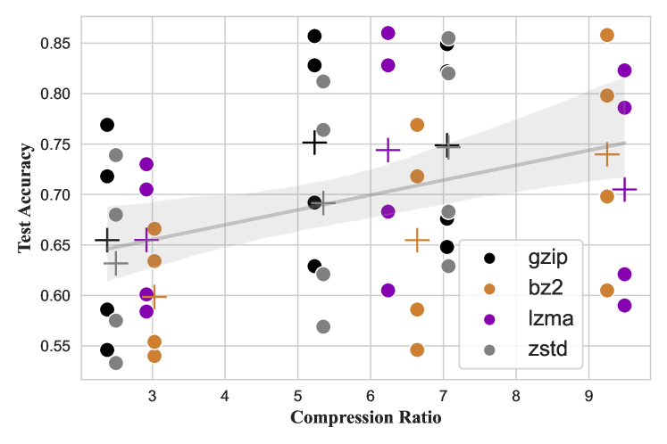
Figure 4: Compression ratio V.S. Test Accuracy across different compressors on three datasets under different shot settings

5.2 Absolute Accuracy

Similarly we evaluate the accuracy of classification with respect to the vocabulary size and we’ve found there is almost no monotonic relation ($r_{s}=0.071)$. With regard to bpc, the monotonic relation is not as strong as the one with the rank percentage ($r_{s}=-0.56$). Considering the effect that vocabulary size has on the relative performance, our method with gzip may be more susceptible to the vocabulary size than neural network methods. To distinguish between a “hard” dataset and an “easy” one, we average all models’ accuracies. The dataset that has the lowest accuracies are 20News and Ohsumed, which are two datasets that have the longest average length of texts.

5.3 Using Other Compressors

With compressor-based distance metrics we can use any compressor. Because of the large size of the test set of the datasets, we randomly chose 1,000 test samples to evaluate and repeat the experiments for each setting five times to calculate the mean and 95% confidence interval.

We carry out experiments on other three compressors: bz2, lzma and zstandard under the few-shot setting. Each of them has different underlying algorithms from gzip. bz2 uses Burrows-Wheeler algorithm to permute the order of characters in the strings to create more repeated “substrings” that can be compressed. That’s one of the reasons why bz2 has a higher compression ratio (e.g., it can achieve 2.57 bpc on AGNews while gzip can achieve only 3.38 bpc). lzma is based on LZ77, a dictionary-based compression algorithm, where the idea is to use (offset, length) to represent the n-gram that has previously appeared in the search buffer. lzma then uses range coding to further encode (offset, length). Similarly, gzip uses DEFLATE algorithm, which also uses LZ77 and instead of range coding, it takes advantage of Huffman coding to further encode (offset, length). zstandard (zstd) is a new compression algorithm that’s built on LZ77, Huffman coding as well as Asymmetric Numeral Systems (ANS) Duda (2009). We pick zstd to evaluate for its fast speed, with close compression rate to gzip. A competitive result may indicate it can be used to speed up the classification.

We plot all the test accuracy in Figure 4 with the compression ratio for each compressor. Compression ratio is calculated by $\frac{\text{original size}}{\text{compressed size}}$, so the larger the compression ratio is, the more a compressor can compress. We use compression ratio instead of bpc here as the latter one is too close to each other and cannot be differentiated from one another. Markers of ‘+’ represents the mean of each compressor’s test accuracy across different shot settings. The dataset is not explicitly labeled but we can tell that there are roughly three clusters in the plot. AGNews is the cluster with the lowest compression ratio and SogouNews is the one with the highest compression ratio. Note that gzip and zstd with compression ratio of about 7 belongs to the SogouNews result.

On SogouNews, both gzip and zstd have the compression ratio equal to about 7; bz2 and lzma have the compression ratio over 9. The difference of accuracy is more obvious on the AGNews and DBpedia with bz2 being the worst-performing compressor. This is counterintuitive, as a compressor with a higher compression ratio suggests that it can approximate Kolmogorov complexity better, and bz2 has a higher compression ratio. We conjecture it may be because in practice, Burrows-Wheeler algorithm used by bz2 dismisses the information of character order. This is shown more clearly in Figure 4 — bz2 is always lower than the regression line. In general, gzip achieves a relatively high and stable accuracy across three datasets. lzma is competitive with gzip but the speed is much slower.

We’ve found in Section 5.1 that for a single compressor, the easier a dataset can compress, the more probable it can achieve a higher accuracy than deep learning models. Here we investiage the correlation across compressors. We’ve found the compression ratio and test accuracy has a moderate monotonic and linear correlation and as the shot number increases, the linear correlation is more obvious with $r_{s}=0.605$ for all shot settings and Pearson correlation $r_{p}=0.575,0.638,0.691,0.719$ respectively on 5, 10, 50 and 100 setting across four compressors. Combining the special case of bz2 with the linear correlation between compression ratio and test accuracy, we know that in general a compressor with a high compression ratio can perform better on a more compressible dataset. But the actual compression algorithm still has its effect on the test accuracy despite the high compression ratio.

Method	AGNews	SogouNews	DBpedia	YahooAnswers
gzip(ce)	0.739 $\pm$0.046	0.741 $\pm$0.076	0.880 $\pm$0.010	0.408 $\pm$0.012
gzip($k$NN)	0.752 $\pm$0.041	0.862 $\pm$0.033	0.852 $\pm$0.008	0.352 $\pm$0.014

Table 6: Comparison with other compressor-based methods under the 100-shot setting.

5.4 Using Other Compressor-Based Methods

The distance metric used by previous work Marton et al. (2005); Russell (2010) is mainly $C(d_{c}d_{u})-C(d_{c})$ as we mention in Section 2.1. Although using this distance metric is faster than pair-wise distance matrix computation on small datasets, it has several drawbacks: (1) Most compressors have a limited “size”, for gzip it’s the sliding window size that can be used to search back of the repeated string while for lzma it’s the dictionary size it can keep record of. This means even if there are large number of training samples, the compressor cannot take full advantage of those samples; (2) When $d_{c}$ is large, compressing $d_{c}d_{u}$ can be really slow and this slowness cannot be solved by parallelization. These two main drawbacks stop this method to be applied to a really large dataset. Thus, we randomly pick 1000 test samples and 100-shot from each class in training samples to compare these two methods. In Table 6, “gzip (ce)” means using the cross entropy $C(d_{c}d_{u})-C(d_{c})$ while “gzip ($k$NN)” refers to our method. We carry our each experiment for five times and calculate the mean and 95% confidence interval. On AGNews and SogouNews using $k$NN and NCD is better than using cross entropy. The reason for the large accuracy gap between them on SogouNews is probably because each instance in SogouNews is very long, causing about 11.2K per sample, while gzip typically has 32K window size only. Only concatenation a few samples makes the compression ineffective. The cross-entropy method does perform very well on YahooAnswers, which may benefit from using multiple references in the single category as YahooAnswers is a divergent dataset created by numerous online users.

We also test the performance of compressor-based cross entropy method on full AGNews dataset as it is a relatively smaller one with shorter single instance. The accuracy is 0.745, not much higher than 100-shot setting, which further confirms that using $C(d_{c}d_{u})-C(d_{c})$ as a distance metric cannot take full advantage of the large datasets.

6 Conclusions and Future Work

In this paper, we use gzip together with a compressor-based distance metric to achieve classification accuracy comparable to neural network classifiers on in-distributed datasets and outperform pre-trained models on out-of-distributed datasets. We also show the effectiveness of using this method in few-shot scenarios. In future works, we will extend this work by generalizing gzip to neural compressors on text, as recent studies Jiang et al. (2022) show that combining neural compressors that derived from deep latent variables models with compressor-based distance metrics for image classification can even outperform semi-supervised methods.

Appendix A Derivation of NCD

Recall that information distance $E(x,y)$ is:

$$E(x,y) =\max\{K(x|y),K(y|x)\}$$ (4)

$$=K(xy)-\min\{K(x),K(y)\}$$ (5)

$E(x,y)$ equates the similarity between two objects with the existence of a program that can convert one to another. The simpler the converting program is, the more similar the objects are. For example, the negative of an image is very similar to the original one as the transformation can be simply described as “inverting the color of the image”.

In order to compare the similarity, relative distance is preferred. Vitányi et al. (2009) propose a normalized version of $E(x,y)$ called Normalized Information Distance (NID).

Definition 1 (NID)

NID is a function: $\Omega\times\Omega\rightarrow[0,1]$, where $\Omega$ is a non-empty set, defined as:

$$\text{NID}(x,y)=\frac{\max\{K(x|y),K(y|x)\}}{\max\{K(x),K(y)\}}.$$ (6)

Equation 6 can be interpreted as follows: Given two sequences $x$, $y$, $K(y)\geq K(x)$:

$$\text{NID}(x,y)=\frac{K(y)-I(x:y)}{K(y)}=1-\frac{I(x:y)}{K(y)},$$ (7)

where $I(x:y)=K(y)-K(y|x)$ means the mutual algorithmic information. $\frac{I(x:y)}{K(y)}$ means the shared information (in bits) per bit of information contained in the most informative sequence, and  Equation 7 here is a specific case of Equation 6.

Normalized Compression Distance (NCD) is a computable version of NID based on real-world compressors. In this context, $K(x)$ can be viewed as the length of $x$ after being maximally compressed. Suppose we have $C(x)$ as the length of compressed $x$ produced by a real-world compressor, then NCD is defined as:

$$\text{NCD}(x,y)=\frac{C(xy)-\min\{C(x),C(y)\}}{\max\{C(x),C(y)\}}.$$ (8)

NCD is thus computable in that it not only uses compressed length to approximate $K(x)$ but also replaces conditional Kolmogorov complexity with $C(xy)$ that only needs a simple concatenation of $x,y$.

Appendix B Implementation Details

We use different hyper-parameters for full-dataset setting and few-shot setting.

For both LSTM, Bi-LSTM+Attn, fasttext, we use embedding size $=256$, dropout rate $=0.3$. For full-dataset setting, the learning rate is set to be $0.001$ and decay rate $=0.9$ for Adam optimizer Kingma and Ba (2015), number of epochs $=20$, with batch size $=64$; for few-shot setting, the learning rate $=0.01$, the decay rate $=0.99$, batch size $=1$, number of epochs $=50$ for 50-shot and 100-shot, epoch $=80$ for 5-shot and 10-shot. For LSTM and Bi-LSTM+Attn, we set RNN layer $=1$, hidden size $=64$. For fasttext, we use 1 hidden layer whose dimension is set to be 10.

For HAN, we use 1 layer for both word-level RNN and sentence-level RNN, the hidden size of both of them are set to 50, the hidden sizes of both attention layers are set to be 100. It’s trained with batch size $=256$, $0.5$ decay rate for $6$ epochs.

For BERT, the learning rate is set to be $2e-5$ and the batch size is set to be $128$ for English and SogouNews while for low-resource languages, we set learning rate to be $1e-5$ with batch size to be 16 for 5 epochs. We use transformers library for BERT’s implementation and specifically we use bert-base-uncased checkpoint for BERT and bert-base-multilingual-uncased for mBERT.

For charCNN and textCNN, we use the same hyper-parameters setting in Adhikari et al. (2019b) except when in the few-shot learning setting, we reduce the batch size to $1$, reducing the learning rate to $1e-4$ and increase the number of epochs to $60$. For VDCNN, we use the shallowest $9$-layer version with embedding size set to be $16$, batch size set to be $64$ learning rate set to be $1e-4$ for full-dataset setting and batch size $=1$, epoch number $=60$ for few-shot setting. For RCNN, we use embedding size $=256$, hidden size of RNN $=256$, learning rate $=1e-3$ and same batch size and epoch setting as VDCNN for full-dataset and few-shot settings.

For pre-processing, we don’t use any pre-trained word embedding for any word-based models. Neither do we use data augmentation during the training. The procedures of tokenization for both word-level and character-level, padding for batch processing are, however, inevitable.

For all zero-training methods, the only hyper-parameter is $k$. We set $k=2$ for all the methods on all the datasets and we report the maximum possible accuracy getting from the experiments for each method. For Sentence-BERT, we use the “paraphrase-MiniLM-L6-v2” checkpoint.

For neural network methods, we use publicly available code for charCNN and textCNN implemented by Adhikari et al. (2019b), and we use Wolf et al. (2020) for BERT.

Our method only requires CPUs and we use 8-core CPUs to take advantage of multi-processing. The time of calculating distance matrix using gzip takes about half an hour on AGNews, two days on DBpedia and SogouNews, six days on YahooAnswers.

All the datasets can be downloaded from torchtext, text categorization corpora and hugging face datasets (Kinyarwanda and Kirundi News, Swahili News, Dengue Filipino).

Appendix C Few-Shot Results

The exact numerical value of accuracy shown in Figure 1 is listed in three tables below.

Dataset	AGNews
#Shot	5	10	50	100
fasttext	0.273 $\pm$0.021	0.329 $\pm$0.036	0.550 $\pm$0.008	0.684 $\pm$0.010
Bi-LSTM+Attn	0.269 $\pm$0.022	0.331 $\pm$0.028	0.549 $\pm$0.028	0.665 $\pm$0.019
HAN	0.274 $\pm$0.024	0.289 $\pm$0.020	0.340 $\pm$0.073	0.548 $\pm$0.031
W2V	0.388 $\pm$0.186	0.546 $\pm$0.162	0.531 $\pm$0.272	0.395 $\pm$0.089
BERT	0.803 $\pm$0.026	0.819 $\pm$0.019	0.869 $\pm$0.005	0.875 $\pm$0.005
SentBERT	0.716 $\pm$0.032	0.746 $\pm$0.018	0.818 $\pm$0.008	0.829 $\pm$0.004
gzip	0.587 $\pm$0.048	0.610 $\pm$0.034	0.699 $\pm$0.017	0.741 $\pm$0.007

Table 7: Few-Shot result on AG News

Dataset	DBpedia
#Shot	5	10	50	100
fasttext	0.475 $\pm$0.041	0.616 $\pm$0.019	0.767 $\pm$0.041	0.868 $\pm$0.014
Bi-LSTM+Attn	0.506 $\pm$0.041	0.648 $\pm$0.025	0.818 $\pm$0.008	0.862 $\pm$0.005
HAN	0.350 $\pm$0.012	0.484 $\pm$0.010	0.501 $\pm$0.003	0.835 $\pm$0.005
W2V	0.325 $\pm$0.113	0.402 $\pm$0.123	0.675 $\pm$0.05	0.787 $\pm$0.015
BERT	0.964 $\pm$0.041	0.979 $\pm$0.007	0.986 $\pm$0.002	0.987 $\pm$0.001
SentBERT	0.730 $\pm$0.008	0.746 $\pm$0.018	0.819 $\pm$0.008	0.829 $\pm$0.004
gzip	0.622 $\pm$0.022	0.701 $\pm$0.021	0.825 $\pm$0.003	0.857 $\pm$0.004

Table 8: Few-Shot result on DBpedia

Dataset	SogouNews
#Shot	5	10	50	100
fasttext	0.545 $\pm$0.053	0.652 $\pm$0.051	0.782 $\pm$0.034	0.809 $\pm$0.012
Bi-LSTM+Attn	0.534 $\pm$0.042	0.614 $\pm$0.047	0.771 $\pm$0.021	0.812 $\pm$0.008
HAN	0.425 $\pm$0.072	0.542 $\pm$0.118	0.671 $\pm$0.102	0.808 $\pm$0.020
W2V	0.141 $\pm$0.005	0.124 $\pm$0.048	0.133 $\pm$0.016	0.395 $\pm$0.089
BERT	0.221 $\pm$0.041	0.226 $\pm$0.060	0.392 $\pm$0.276	0.679 $\pm$0.073
SentBERT	0.485 $\pm$0.043	0.501 $\pm$0.041	0.565 $\pm$0.013	0.572 $\pm$0.003
gzip	0.649 $\pm$0.061	0.741 $\pm$0.017	0.833 $\pm$0.007	0.867 $\pm$0.016

Table 9: Few-Shot result on SogouNews

References

- Adhikari et al. (2019a) Ashutosh Adhikari, Achyudh Ram, Raphael Tang, and Jimmy Lin. 2019a. Docbert: Bert for document classification. arXiv preprint arXiv:1904.08398.
- Adhikari et al. (2019b) Ashutosh Adhikari, Achyudh Ram, Raphael Tang, and Jimmy Lin. 2019b. Rethinking complex neural network architectures for document classification. In Proceedings of the 2019 Conference of the North American Chapter of the Association for Computational Linguistics: Human Language Technologies, Volume 1 (Long and Short Papers), pages 4046–4051.
- Bennett et al. (1998) Charles H Bennett, Péter Gács, Ming Li, Paul MB Vitányi, and Wojciech H Zurek. 1998. Information distance. IEEE Transactions on information theory, 44(4):1407–1423.
- Bowman et al. (2015) Samuel Bowman, Gabor Angeli, Christopher Potts, and Christopher D Manning. 2015. A large annotated corpus for learning natural language inference. In Proceedings of the 2015 Conference on Empirical Methods in Natural Language Processing, pages 632–642.
- Chen et al. (2004) Xin Chen, Brent Francia, Ming Li, Brian Mckinnon, and Amit Seker. 2004. Shared information and program plagiarism detection. IEEE Transactions on Information Theory, 50(7):1545–1551.
- Chen et al. (1999) Xin Chen, Sam Kwong, and Ming Li. 1999. A compression algorithm for dna sequences and its applications in genome comparison. Genome informatics, 10:51–61.
- Conneau et al. (2017) Alexis Conneau, Holger Schwenk, Loïc Barrault, and Yann Lecun. 2017. Very deep convolutional networks for text classification. In Proceedings of the 15th Conference of the European Chapter of the Association for Computational Linguistics: Volume 1, Long Papers, pages 1107–1116.
- Coutinho and Figueiredo (2015) David Pereira Coutinho and Mario AT Figueiredo. 2015. Text classification using compression-based dissimilarity measures. International Journal of Pattern Recognition and Artificial Intelligence, 29(05):1553004.
- Devlin et al. (2019) Jacob Devlin, Ming-Wei Chang, Kenton Lee, and Kristina Toutanova. 2019. Bert: Pre-training of deep bidirectional transformers for language understanding. In Proceedings of the 2019 Conference of the North American Chapter of the Association for Computational Linguistics: Human Language Technologies, Volume 1 (Long and Short Papers), pages 4171–4186.
- Duda (2009) Jarek Duda. 2009. Asymmetric numeral systems. arXiv preprint arXiv:0902.0271.
- Frank et al. (2000) Eibe Frank, Chang Chui, and Ian H Witten. 2000. Text categorization using compression models.
- Hochreiter and Schmidhuber (1997) Sepp Hochreiter and Jürgen Schmidhuber. 1997. Long short-term memory. Neural computation, 9(8):1735–1780.
- Jiang et al. (2022) Zhiying Jiang, Yiqin Dai, Ji Xin, Ming Li, and Jimmy Lin. 2022. Few-shot non-parametric learning with deep latent variable model. Advances in Neural Information Processing Systems (NeurIPS).
- Joulin et al. (2017) Armand Joulin, Edouard Grave, and Piotr Bojanowski Tomas Mikolov. 2017. Bag of tricks for efficient text classification. EACL 2017, page 427.
- Kasturi and Markov (2022) Nitya Kasturi and Igor L Markov. 2022. Text ranking and classification using data compression. In I (Still) Can’t Believe It’s Not Better! Workshop at NeurIPS 2021, pages 48–53. PMLR.
- Kawakami (2008) Kazuya Kawakami. 2008. Supervised sequence labelling with recurrent neural networks. Ph. D. thesis.
- Kenton and Toutanova (2019) Jacob Devlin Ming-Wei Chang Kenton and Lee Kristina Toutanova. 2019. Bert: Pre-training of deep bidirectional transformers for language understanding. In Proceedings of NAACL-HLT, pages 4171–4186.
- Keogh et al. (2004) Eamonn Keogh, Stefano Lonardi, and Chotirat Ann Ratanamahatana. 2004. Towards parameter-free data mining. In Proceedings of the tenth ACM SIGKDD international conference on Knowledge discovery and data mining, pages 206–215.
- Khmelev and Teahan (2003) Dmitry V Khmelev and William J Teahan. 2003. A repetition based measure for verification of text collections and for text categorization. In Proceedings of the 26th annual international ACM SIGIR conference on Research and development in informaion retrieval, pages 104–110.
- Kingma and Ba (2015) Diederik P Kingma and Jimmy Ba. 2015. Adam: A method for stochastic optimization. In ICLR (Poster).
- Kolmogorov (1963) Andrei N Kolmogorov. 1963. On tables of random numbers. Sankhyā: The Indian Journal of Statistics, Series A, pages 369–376.
- Lai et al. (2015) Siwei Lai, Liheng Xu, Kang Liu, and Jun Zhao. 2015. Recurrent convolutional neural networks for text classification. In Twenty-ninth AAAI conference on artificial intelligence.
- LeCun et al. (2015) Yann LeCun, Yoshua Bengio, and Geoffrey Hinton. 2015. Deep learning. nature, 521(7553):436–444.
- Li et al. (2004) Ming Li, Xin Chen, Xin Li, Bin Ma, and Paul MB Vitányi. 2004. The similarity metric. IEEE transactions on Information Theory, 50(12):3250–3264.
- Li et al. (2022) Qian Li, Hao Peng, Jianxin Li, Congying Xia, Renyu Yang, Lichao Sun, Philip S Yu, and Lifang He. 2022. A survey on text classification: From traditional to deep learning. ACM Transactions on Intelligent Systems and Technology (TIST), 13(2):1–41.
- Marton et al. (2005) Yuval Marton, Ning Wu, and Lisa Hellerstein. 2005. On compression-based text classification. In European Conference on Information Retrieval, pages 300–314. Springer.
- Mikolov et al. (2013) Tomas Mikolov, Kai Chen, Greg Corrado, and Jeffrey Dean. 2013. Efficient estimation of word representations in vector space. arXiv preprint arXiv:1301.3781.
- Nogueira et al. (2020) Rodrigo Nogueira, Zhiying Jiang, Ronak Pradeep, and Jimmy Lin. 2020. Document ranking with a pretrained sequence-to-sequence model. In Findings of the Association for Computational Linguistics: EMNLP 2020, pages 708–718.
- Reimers and Gurevych (2019) Nils Reimers and Iryna Gurevych. 2019. Sentence-bert: Sentence embeddings using siamese bert-networks. In Proceedings of the 2019 Conference on Empirical Methods in Natural Language Processing and the 9th International Joint Conference on Natural Language Processing (EMNLP-IJCNLP), pages 3982–3992.
- Russell (2010) Stuart J Russell. 2010. Artificial intelligence a modern approach. Pearson Education, Inc.
- Schuster and Paliwal (1997) Mike Schuster and Kuldip K Paliwal. 1997. Bidirectional recurrent neural networks. IEEE transactions on Signal Processing, 45(11):2673–2681.
- Shen et al. (2018) Dinghan Shen, Guoyin Wang, Wenlin Wang, Martin Renqiang Min, Qinliang Su, Yizhe Zhang, Chunyuan Li, Ricardo Henao, and Lawrence Carin. 2018. Baseline needs more love: On simple word-embedding-based models and associated pooling mechanisms. In Proceedings of the 56th Annual Meeting of the Association for Computational Linguistics (Volume 1: Long Papers), pages 440–450.
- Teahan and Harper (2003) William J Teahan and David J Harper. 2003. Using compression-based language models for text categorization. In Language modeling for information retrieval, pages 141–165. Springer.
- Vitányi et al. (2009) Paul MB Vitányi, Frank J Balbach, Rudi L Cilibrasi, and Ming Li. 2009. Normalized information distance. In Information theory and statistical learning, pages 45–82. Springer.
- Wang et al. (2016) Yequan Wang, Minlie Huang, Xiaoyan Zhu, and Li Zhao. 2016. Attention-based lstm for aspect-level sentiment classification. In Proceedings of the 2016 conference on empirical methods in natural language processing, pages 606–615.
- Williams et al. (2018) Adina Williams, Nikita Nangia, and Samuel Bowman. 2018. A broad-coverage challenge corpus for sentence understanding through inference. In Proceedings of the 2018 Conference of the NAACL-HLT, Volume 1 (Long Papers), pages 1112–1122, New Orleans, Louisiana. Association for Computational Linguistics.
- Wolf et al. (2020) Thomas Wolf, Lysandre Debut, Victor Sanh, Julien Chaumond, Clement Delangue, Anthony Moi, Pierric Cistac, Tim Rault, Rémi Louf, Morgan Funtowicz, et al. 2020. Transformers: State-of-the-art natural language processing. In Proceedings of the 2020 conference on empirical methods in natural language processing: system demonstrations, pages 38–45.
- Yang et al. (2016) Zichao Yang, Diyi Yang, Chris Dyer, Xiaodong He, Alex Smola, and Eduard Hovy. 2016. Hierarchical attention networks for document classification. In Proceedings of the 2016 conference of the North American chapter of the association for computational linguistics: human language technologies, pages 1480–1489.
- Yao et al. (2019) Liang Yao, Chengsheng Mao, and Yuan Luo. 2019. Graph convolutional networks for text classification. In Proceedings of the AAAI conference on artificial intelligence, volume 33, pages 7370–7377.
- Yu et al. (2021) Yaodong Yu, Heinrich Jiang, Dara Bahri, Hossein Mobahi, Seungyeon Kim, Ankit Singh Rawat, Andreas Veit, and Yi Ma. 2021. An empirical study of pre-trained vision models on out-of-distribution generalization. In NeurIPS 2021 Workshop on Distribution Shifts: Connecting Methods and Applications.
- Zhang et al. (2021) Haode Zhang, Yuwei Zhang, Li-Ming Zhan, Jiaxin Chen, Guangyuan Shi, Xiao-Ming Wu, and Albert YS Lam. 2021. Effectiveness of pre-training for few-shot intent classification. In Findings of the Association for Computational Linguistics: EMNLP 2021, pages 1114–1120.
- Zhang et al. (2015) Xiang Zhang, Junbo Zhao, and Yann LeCun. 2015. Character-level convolutional networks for text classification. Advances in neural information processing systems, 28.