Identification of time-varying counterfactual parameters in nonlinear panel models

Abstract

We develop a general framework for the identification of counterfactual parameters in a class of nonlinear semiparametric panel models with fixed effects and time effects. Our method applies to models for discrete outcomes (e.g., two-way fixed effects binary choice) or continuous outcomes (e.g., censored regression), with discrete or continuous regressors. Our results do not require parametric assumptions on the error terms or time-homogeneity on the outcome equation. Our main results focus on static models, with a set of results applying to models without any exogeneity conditions. We show that the survival distribution of counterfactual outcomes is identified (point or partial) in this class of models. This parameter is a building block for most partial and marginal effects of interest in applied practice that are based on the average structural function as defined by Blundell and Powell (2003, 2004). To the best of our knowledge, ours are the first results on average partial and marginal effects for binary choice and ordered choice models with two-way fixed effects and non-logistic errors.

JEL classification: C14; C23; C41.
Keywords: index model; panel data; fixed effects; average structural function; semiparametric; binary choice; discrete choice; censored regression.

1 Introduction

We study counterfactual or policy parameters for nonlinear panel models with structural equation

$$Y_{it}\left(x\right) =h_{t}\left(\alpha_{i}+x\beta-U_{it}\right),\text{ $t=1,2,\dots,T$,}$$ (1)

where $i$ indexes individual units, $t$ indexes time, $h_{t}$ is a weakly-monotone transformation function that can vary over $t$ in an unrestricted way, $\beta\in\mathbb{R}^{k}$ is a vector of regression coefficients, $\alpha_{i}$ is an individual-specific effect, and $U_{it}$ is a stochastic error term. For each unit $i$, we observe covariates $X_{it}$, $t=1,\dots,T$. The dependence between $\alpha_{i}$ and $X_{i}=\left(X_{i1},\dots,X_{iT}\right)$ is left unrestricted, so that $\alpha_{i}$ is a fixed effect, c.f., e.g., Graham and Powell (2012). The class of models with outcome equation as in (1) includes the binary choice model with two-way fixed effects, the ordered choice model with fixed effects and time-varying cut-offs, the censored regression model with time-varying censoring, and various transformation models for continuous dependent variables.

For a subpopulation of individuals defined by their sequence of regressor values $X_{i}$, our parameter of interest is the counterfactual survival probability:

$$\tau_{t,x,y}\left(X_{i}\right)\equiv P\left(\left.Y_{it}\left(x\right)\geq y\right|X_{i}\right),\text{ $t=1,2,\dots,T$,}$$ (2)

where $Y_{it}\left(x\right)$ is given by (1), $x$ is a fixed counterfactual value of the period-$t$ regressors, and $y\in\underline{\mathcal{Y}}\equiv\mathcal{Y}\setminus\text{inf}\mathcal{Y}$ is a fixed cut-off value, where $\mathcal{Y}\subseteq\mathbb{R}$ denotes the support of the observed $Y_{it}=Y_{it}\left(X_{it}\right)$. The parameter in (2) is a building block for most partial and marginal effects of interest in applied practice that are based on the average structural function (ASF) as defined in the pioneering work of Blundell and Powell (2003, 2004). For example, when $Y_{it}\left(x\right)$ is non-negative , the ASF at time $t$ can be obtained as:

$$ASF_{t}\left(x\right)=\mathbb{E}\left[\mathbb{E}\left(\left.Y_{it}\left(x\right)\right|X_{i}\right)\right]=\mathbb{E}\left(\int_{0}^{\infty}\tau_{t,x,y}\left(X_{i}\right)dy\right).$$ (3)

The ASF can then be used to define partial effects based on partial derivatives or marginal effects based on discrete differences, see, e.g., Lin and Wooldridge (2015).

The challenge is to identify (2) in nonlinear panel models with structural equation as in (1) when $\alpha_{i}$ are fixed effects and $T<\infty$. To see that this is challenging, consider the special case of the binary choice model with two-way fixed effects. A recent literature has made progress in identifying certain counterfactual parameters for this model provided that the error terms follow a standard logistic distribution, see e.g. Aguirregabiria and Carro (2021), Davezies et al. (2022), Dobronyi et al. (2021).

A separate literature provides identification results under time-homogeneity assumptions that do not allow for arbitrary time-effects, see the benchmark results in Hoderlein and White (2012), Chernozhukov et al. (2013), and Chernozhukov et al. (2015). To the best of our knowledge, nothing is known about the identification of the ASF for the binary choice model with two way fixed effects without logistic errors.

We derive (partial) identification results for (2) without parametric restrictions on the distribution of $U_{it}$ for panel models with outcome equation as in (1). Our results are for short-$T$. Relevant examples of models to which our results apply are (i) binary choice with two-way fixed effects and nonlogistic errors, (ii) ordered choice with time-varying thresholds, (iii) censored regression with time-varying censoring. Additionally, since (2) varies over time whenever $h_{t}$ is time-varying, policy parameters that are functionals of (2) are also time-varying.

For nonseparable panel models with fixed effects, the results in benchmark work such as Hoderlein and White (2012), Chernozhukov et al. (2013), and Chernozhukov et al. (2015) establish limitations on what can be learned from panel data in terms of counterfactual parameters. By imposing additional structure on the latent outcome, such as additivity in a linear index and the fixed effects, we show that (partial) identification of counterfactual parameters can be obtained without time-homogeneity assumptions on the outcome equation and no parametric assumptions on the distribution of the error terms. Because we make no time-homogeneity assumptions on $h_{t}$, the counterfactual parameters can vary over time in an arbitrary way. To the best of our knowledge, it is the combination of time-varyingness of the outcome equation (hence, of the counterfactual parameters) and no parametric distributional assumptions on the error terms that constitutes our contribution relative to the literature on partial effects in nonlinear panel models with fixed effects.

For our results, we treat $\beta$ and $h_{t}$ as given, i.e. either known or previously point- or partially-identified. Our key insight is that the linear index structure allows us to classify each observed probability at time $s$,

$$P\left(\left.Y_{is}\geq y^{\prime}\right|X_{i}\right),\;s=1,\dots,T,y^{\prime}\in\underline{\mathcal{Y}},$$ (4)

as either an upper bound on $\tau_{t,x,y}\left(X_{i}\right)$, a lower bound on $\tau_{t,x,y}\left(X_{i}\right)$, or both. We show that (4) is an upper bound only if the observed index at time $s$, $X_{is}\beta-h_{s}^{-}\left(y\right)$, is at least the counterfactual index at time $t$, $x\beta-h_{t}^{-}\left(y\right)$; and a lower bound only if the observed index at time $s$ is at most the counterfactual index at time $t$. Without any additional time-stationarity or exogeneity assumptions, bounds on the period-$t$ counterfactual probability $\tau_{t,x,y}\left(X_{i}\right)$ can be constructed from the period-$t$ observed probabilities $P\left(\left.Y_{it}\geq y^{\prime}\right|X_{i}\right)$, $y^{\prime}\in\underline{\mathcal{Y}}$. Under a conditional time-stationarity assumption on the errors, outcomes from all periods are informative for the period-$t$ counterfactual probability. The bounds under conditional time-stationarity are tighter than those without exogeneity assumptions. Point identification is obtained when the transformation function $h_{t}$ is invertible or when the counterfactual index equals one of the observed indices.

The remainder of this paper is organized as follows. Section 2 presents our main results: Section 2.1 constructs bounds without any additional time-stationarity or exogeneity assumptions, while Section 2.2 constructs bounds under a conditional time-stationarity assumption on the error terms. Section 3 applies our results to a few examples: binary choice model, ordered choice model, and censored regression. We present a numerical experiment for the binary choice model in Section 4.1 and one for the ordered choice model in Section 4.2. All proofs and an additional numerical experiment can be found in the Appendix.

2 Main results

We provide two results on the identification of $\tau_{t,x,y}$ defined in (2). Our first result in Theorem 1 provides bounds on $\tau_{t,x,y}$ without imposing any exogeneity assumptions or time-stationarity assumptions on $U_{it},\,X_{i}$. Our second result in Theorem 2 uses a conditional time-stationarity assumption on $\left.U_{it}\right|\alpha_{i},X_{i}$ to tighten those bounds. Conditioning on the sequence $X_{i}$ allows us to identify the same parameter, $\tau_{t,x,y}$, across different exogeneity and time-stationarity assumptions.

The following two assumptions are maintained throughout the paper:

Assumption 1.

(i) The distribution of panel data $\left(X_{i1},\cdots,X_{iT},Y_{i1},\cdots,Y_{iT}\right)$ is observed, where $Y_{it}=Y_{it}\left(X_{it}\right)$ is generated by (1); (ii) $\beta$ and $h_{t}$ in (1) are either known, point-identified, or partially-identified.

Footnote 9 lists work that provides sufficient assumptions for either the point- or the partial-identification of $\beta$ and $h_{t}$.

Assumption 2.

For each $t$, $h_{t}:\mathbb{R}\rightarrow\mathcal{Y}\subseteq\mathbb{R}$ is weakly-monotone and right-continuous.

Assumption 2 does not restrict the way that $h_{t}$ can vary over $t$. Our results apply to the case of time-invariant $h_{t}=h$, in which case parameters such as (2) and (3) are also time-invariant. This assumption allows $h_{t}$ to have flat parts and jumps, or to be continuous. Hence, our setting accommodates both discrete and continuous outcomes.

Given Assumption 2, we define the generalized inverse of $h_{t}$ as:

$$h_{t}^{-}\left(y\right)\equiv\inf\left\{y^{*}:h_{t}\left(y^{*}\right)\geq y\right\},y\in\mathcal{\underline{\mathcal{Y}}},$$ (5)

i.e. it is the smallest value of the latent variable that yields a value of the observed outcome $Y_{t}\geq y$.

For what follows we fix $t,x$ and we fix $y\in\underline{\mathcal{Y}}$.

2.1 No additional exogeneity or time-stationarity assumptions

For our first set of results, we define the following sets:

$$\mathcal{Y}_{L} \equiv\left\{y^{\prime}\in\underline{\mathcal{Y}}:X_{it}\beta-h_{t}^{-}\left(y^{\prime}\right)\leq x\beta-h_{t}^{-}\left(y\right)\right\},$$ (6)

$$\mathcal{Y}_{U} \equiv\left\{y^{\prime}\in\underline{\mathcal{Y}}:X_{it}\beta-h_{t}^{-}\left(y^{\prime}\right)\geq x\beta-h_{t}^{-}\left(y\right)\right\}.$$ (7)

The set $\mathcal{Y}_{L}$ collects the values $y^{\prime}\in\underline{\mathcal{Y}}$ for which the counterfactual index at time $t$, $x\beta-h_{t}^{-}\left(y\right)$, is greater than the observed index at time $t$, $X_{it}\beta-h_{t}^{-}\left(y^{\prime}\right)$, while $\mathcal{Y}_{U}$ collects the values $y^{\prime}\in\underline{\mathcal{Y}}$ for which the counterfactual index at time $t$ is smaller than the observed index at time $t$. Note that $\mathcal{Y}_{L}\cup\mathcal{Y}_{U}=\underline{\mathcal{Y}}$.

Theorem 1.

Let $Y_{it}$ follow (1) and let Assumptions 1 and 2 hold. Then, for given values of $\beta$ and $h_{t}$,

$$\tau_{t,x,y}\left(X_{i}\right)\in\left[\sup_{y^{\prime}\in\mathcal{Y}_{L}}P\left(\left.Y_{it}\geq y^{\prime}\right|X_{i}\right),\inf_{y^{\prime}\in\mathcal{Y}_{U}}P\left(\left.Y_{it}\geq y^{\prime}\right|X_{i}\right)\right]\cap\left[0,1\right],$$ (8)

using the convention that $\sup\emptyset=-\infty$ and $\inf\emptyset=+\infty$.

Theorem 1 uses the linear-index structure of (1) and knowledge of $\beta$ and $h_{t}$ to classify $P\left(\left.Y_{it}\geq y^{\prime}\right|X_{i}\right)$ as a lower (upper) bound on $\tau_{t,x,y}\left(X_{i}\right)$ for any value of $y^{\prime}\in\underline{\mathcal{Y}}$. By varying $y^{\prime}\in\underline{\mathcal{Y}},$ we obtain the sets $\mathcal{Y}_{L}$ ($\mathcal{Y}_{U})$ of values $y^{\prime}$ that provide lower (upper) bounds. Equation (8) intersects these bounds. Since $\mathcal{Y}_{L}\cup\mathcal{Y}_{U}=\underline{\mathcal{Y}}$, every value of $y^{\prime}$ provides an upper bound, a lower bound, or both. Note that since either $\mathcal{Y}_{L}$ or $\mathcal{Y}_{U}$ can be empty, the trivial lower (upper) bound is selected by the intersection with $\left[0,1\right]$.

Section 3 applies Theorem 1 to binary choice, ordered choice, and censored regression. In the case of binary choice, the bounds of Theorem 1 simplify significantly. In that case, $P\left(\left.Y_{it}\geq 1\right|X_{i}\right)$ provides an upper bound for $P\left(\left.Y_{it}\left(x\right)\geq 1\right|X_{i}\right)$ if $X_{it}\beta>x\beta$, and a lower bound if $X_{it}\beta<x\beta$. When $X_{it}\beta=x\beta$, $P\left(\left.Y_{it}\geq 1\right|X_{i}\right)$ point-identifies $P\left(\left.Y_{it}\left(x\right)\geq 1\right|X_{i}\right)$.

Remark 1.

The result in Theorem 1 is stated for a given value of $\left(\beta,h_{t}\right)$. Thus, the bounds are directly applicable in case where $\left(\beta,h_{t}\right)$ are point-identified. If $\left(\beta,h_{t}\right)$ are partially identified, bounds on $\tau_{t,x,y}\left(X_{i}\right)$ can be obtained by taking the worst-case bounds across parameter values in the identified set.

Remark 2.

The bounds in Theorem 1 do not require any additional exogeneity conditions on $\left(X_{i},U_{i}\right)$ beyond those that may be needed for Assumption (1)(ii). In particular, the bounds are valid for models with strictly or weakly exogenous regressors, with lagged dependent variables, and with endogenous regressors. Likewise, the bounds do not require any time-stationarity assumptions on the distribution of the error terms. In this sense, the bounds are valid for models with errors with time-varying distributions. Finally, separability in $\alpha_{i}$ and $U_{it}$ is not necessary for identification of the counterfactual survival probability, suggesting that our argument can be applied to a more general class of models.

Remark 3.

Point identification occurs in a number of settings. First, when $h_{t}$ is invertible, see Section (3.1). Second, when there exists a $y^{\prime}$ such that

$$h_{t}^{-}\left(y^{\prime}\right)=\left(X_{it}-x\right)\beta+h_{t}^{-}\left(y\right).$$

This can happen, among others, when $y=y^{\prime}$ and $X_{it}=x$ (or $X_{it}\beta=x\beta$). In this case, $y\in\mathcal{Y}_{L}\cap\mathcal{Y}_{U}$ and the upper and lower bounds coincide.

Remark 4.

The bounds in Theorem 1 shrink with the cardinality of $\underline{\mathcal{Y}}$, so that the worst case for our bounds is when the outcomes are binary (worst case here means that, provided failure of point-identification, one of the bounds is always trivial), while the best case is when the outcomes are continuous (best case in the sense that the parameter of interest is always point-identified).

2.2 Conditional time-stationarity

The bounds in Theorem 1 can be wide, for example when the dependent variable has few points of support (see Remark 4). The following assumption obtains tighter bounds by using information across all time periods rather than information from period $t$ only.

Assumption 3.

Conditional time-stationarity: $\left.U_{it}\right|\alpha_{i},X_{i}\stackrel{{\scriptstyle d}}{{=}}\left.U_{i1}\right|\alpha_{i},X_{i}$, for all $t=2,\dots,T$.

Conditional time-stationarity requires that the conditional distribution of the error terms conditional on $\alpha_{i},X_{i}$ be the same in each time period. In Chernozhukov et al. (2013, 2015) and Hoderlein and White (2012) the authors refer to this assumption as both “strict exogeneity” and time-homogeneity of the error terms. Note that the error terms are required to have a time-stationary (“time-homogeneous”) distribution conditional on $\alpha_{i}$ and the entire sequence $X_{i1},\dots,X_{iT}$. The assumption allows for serial correlation in the errors $U_{it}$ and in some components of $X_{i}$, and it leaves the distribution of $\alpha_{i}$ conditional on $X_{i}$ unrestricted. Note that, in our set-up with time-varying structural equation, the conditional distribution of $Y_{it}$ given $X_{i}$ can still vary over time.

Fix $t,x,$$y\in\underline{\mathcal{Y}}$ and define the sets:

$$\mathcal{L} \equiv\left\{\left(s,y^{\prime}\right)\in\left\{1,\cdots,T\right\}\times\mathcal{\underline{\mathcal{Y}}}:X_{is}\beta-h_{s}^{-}\left(y^{\prime}\right)\leq x\beta-h_{t}^{-}\left(y\right)\right\},$$

$$\mathcal{U} \equiv\left\{\left(s,y^{\prime}\right)\in\left\{1,\cdots,T\right\}\times\underline{\mathcal{Y}}:X_{is}\beta-h_{s}^{-}\left(y^{\prime}\right)\geq x\beta-h_{t}^{-}\left(y\right)\right\}.$$

Theorem 2.

Let $Y_{i1},\cdots,Y_{iT}$ follow (1), and let Assumptions (1), 2, and 3 hold. Then, for given values of $\beta$ and $h_{t}$,

$$\tau_{t,x,y}\left(X_{i}\right)\in\left[\sup_{\left(s,y^{\prime}\right)\in\mathcal{L}}P\left(\left.Y_{is}\geq y^{\prime}\right|X_{i}\right),\inf_{\left(s,y^{\prime}\right)\in\mathcal{U}}P\left(\left.Y_{is}\geq y^{\prime}\right|X_{i}\right)\right]\cap\left[0,1\right],$$

using the convention that $\sup\emptyset=-\infty$ and $\inf\emptyset=+\infty$.

As in the case of in Theorem 1, the result above applies directly to point-identified $\beta$ and $h_{t}$. If $\left(\beta,h_{t}\right)$ are partially identified, bounds on $\tau_{t,x,y}\left(X_{i}\right)$ can be obtained by taking the worst-case bounds across parameter values in the identified set.

According to Theorem 2, we can use information from any period $s$ to construct bounds on the counterfactual survival distribution in period $t$. The resulting bounds can be much more informative than those in Theorem 1 without time-stationarity and exogeneity assumptions; this can be seen from the expressions for binary and ordered choice in Section 3, and from the numerical experiments in Section 4. The gains can be substantial, especially if the number of time periods is large, if there is variation in the values of the sequence $X_{i}$, and if there is a large degree of variation over time in $h_{t}$.

Remark 5.

That variation in $h_{t}$ can improve identification is particularly interesting. In related settings, time-homogeneity of the outcome equation, i.e. $h_{t}=h$, has been used for identification of partial effects in panel models. In our setting, time-variation in the structural function can aid identification of partial effects in monotone single-index models. For an example, see our analysis of binary choice models in Section 3.2.

Remark 6.

The best upper and lower bounds can be thought of as, first, choosing the best $y^{\prime}$ for each time period (as in Theorem 1) and then choosing the best time period. Letting

$$\mathcal{Y}_{sL} \equiv\left\{y^{\prime}\in\mathcal{\underline{\mathcal{Y}}}:X_{is}\beta-h_{s}^{-}\left(y^{\prime}\right)\leq x\beta-h_{t}^{-}\left(y\right)\right\},$$

$$\mathcal{Y}_{sU} \equiv\left\{y^{\prime}\in\underline{\mathcal{Y}}:X_{is}\beta-h_{s}^{-}\left(y^{\prime}\right)\geq x\beta-h_{t}^{-}\left(y\right)\right\},$$

we obtain a bound for each time period,

$$\tau_{t,x,y}\left(X_{i}\right)\in\left[\sup_{y^{\prime}\in\mathcal{Y}_{sL}}P\left(\left.Y_{is}\geq y^{\prime}\right|X_{i}\right),\inf_{y^{\prime}\in\mathcal{Y}_{sU}}P\left(\left.Y_{is}\geq y^{\prime}\right|X_{i}\right)\right]\cap\left[0,1\right]$$

and, because this bound applies for each period $s$, we obtain

$$\tau_{t,x,y}\left(X_{i}\right)\in\cap_{s\in\left\{1,\cdots,T\right\}}\left[\sup_{y^{\prime}\in\mathcal{Y}_{sL}}P\left(\left.Y_{is}\geq y^{\prime}\right|X_{i}\right),\inf_{y^{\prime}\in\mathcal{Y}_{sU}}P\left(\left.Y_{is}\geq y^{\prime}\right|X_{i}\right)\right]\cap\left[0,1\right]$$

or

$$\max_{s\in\left\{1,\cdots,T\right\}}\sup_{y^{\prime}\in\mathcal{Y}_{sL}}P\left(\left.Y_{is}\geq y^{\prime}\right|X_{i}\right)\leq\tau_{t,x,y}\left(X_{i}\right)\leq\min_{s\in\left\{1,\cdots,T\right\}}\inf_{y^{\prime}\in\mathcal{Y}_{sU}}P\left(\left.Y_{is}\geq y^{\prime}\right|X_{i}\right).$$

We illustrate this for the binary and ordered choice models in Section 3.

Remark 7.

As in the case of in Theorem 1, the bounds in Theorem 2 do not require separability in $\alpha_{i}$ and $U_{it}$ for identification of the counterfactual survival probability. Thus, our argument may be applied to a more general class of models.

Remark 8.

Theorem 2 updates and replaces the results in Section 3.2 in Botosaru and Muris (2017).

3 Examples

In this section, we apply our results to a number of empirically relevant choices for $h_{t}$. These examples are helpful in understanding how informative our bounds are, and help relate them to existing bounds in the literature derived under related but different conditions.

Let $v\equiv\alpha_{i}+X_{it}\beta-U_{it}$. We start by applying our results to the fixed effects linear transformation model with invertible $h_{t}$. We then study binary choice models with two-way fixed effects $h_{t}\left(v\right)=1\left\{v\geq\lambda_{t}\right\}$, ordered choice models with time-varying thresholds $h_{t}\left(v\right)=\sum_{j=1}^{J}1\left\{v\geq\lambda_{jt}\right\}$, $J\in\mathbb{N},$ and censored regression with $h_{t}\left(v\right)=\max\left\{\lambda_{t},v\right\}$.

3.1 Continuous outcomes and invertible $h_{t}$

Let $h_{t}$ be invertible, so that $h_{t}^{-}=h_{t}^{-1}$. Examples include linear regression with two-way fixed effects, i.e. $h_{t}\left(v\right)=v+\lambda_{t}$; transformation models used in duration analysis; and the Box-Cox transformation model.

Let $h_{t}$ be defined on $\mathbb{R},$or $v\in\mathbb{R}.$ There always exists a $y^{\prime}$ such that

$$y^{\prime} =h_{t}\left(h_{t}^{-1}\left(y\right)+\left(x-X_{it}\right)\beta\right)$$

$$\in\mathcal{Y}_{L}\cap\mathcal{Y}_{U}.$$

Theorem 1 applies and the counterfactual survival probability (2) is point-identified. To see this, consider the argument below:

$$\tau_{t,x,y}\left(X_{i}\right) =P\left(\left.Y_{it}\left(x\right)\geq y\right|X_{i}\right)$$

$$=P\left(\left.\alpha_{i}-U_{it}\geq h_{t}^{-1}\left(y\right)-x\beta\right|X_{i}\right)$$

$$=P\left(\left.\alpha_{i}+X_{it}\beta-U_{it}\geq h_{t}^{-1}\left(y\right)+\left(X_{it}-x\right)\beta\right|X_{i}\right)$$

$$=P\left(\left.Y_{it}\geq h_{t}\left(h_{t}^{-1}\left(y\right)+\left(X_{it}-x\right)\beta\right)\right|X_{i}\right)$$

$$=P\left(\left.Y_{it}\geq y^{\prime}\right|X_{i}\right),$$

where invertibility of $h_{t}$ was used in the second equality.

We are not aware of results for $\tau_{t,x,y}$ – or derived quantities such as partial/marginal effects – for the case considered here, other than those in Botosaru and Muris (2017); Botosaru et al. (2021, 2022).

3.2 Binary choice

The link function

$$h_{t}\left(v\right)=1\left\{v-\lambda_{t}\geq 0\right\}$$

obtains the panel binary choice model with two-way fixed effects with structural function

$$Y_{it}\left(x\right)=1\left\{\alpha_{i}+x\beta-U_{it}-\lambda_{t}\geq 0\right\}.$$ (9)

Our results yield bounds on (2), hence on partial effects, without parametric assumptions on the distribution of the error terms and for a variety of exogeneity conditions. The only existing results without parametric assumptions on the error term that we are aware of are those in Chernozhukov et al. (2013), but those require that regressors be discrete and that $\lambda_{t}=0$ for all $t$.

In what follows, we fix the time period for the counterfactual to $t=1$ and use the abbreviated notation

$$\tau_{x}\left(X_{i}\right)\equiv\tau_{1,x,1}\left(X_{i}\right)=P\left(\left.Y_{i1}\left(x\right)\geq 1\right|X_{i}\right).$$ (10)

For this model, $\underline{\mathcal{Y}}=\left\{1\right\}$ and $h_{t}^{-}\left(1\right)=\lambda_{t}$.

Remark 9.

By removing inf$\mathcal{Y}=0$, we remove $h_{t}^{-}\left(0\right)=-\infty$. This is useful, since, e.g., Theorem 1 asks us to compare $X_{it}\beta-h_{t}^{-}\left(y^{\prime}\right)$ to $x\beta-h_{t}^{-}\left(y\right)$ for all values of $y^{\prime}$ and fixed $x,y,X_{i}$. For the particular case that $y^{\prime}=\text{inf}\mathcal{Y}=0=y$, this obtains $X_{it}\beta+\infty$ and $x\beta+\infty$. Note that we could allow $y^{\prime}\in\mathcal{Y}$ for fixed $y\in\mathcal{\underline{Y}}$, but this would lead to obtaining trivial bounds, i.e. for $y=1$ and $y^{\prime}=0$, $\text{$\tau_{t,x,1}\left(X_{i}\right)$}\leq P\left(\left.Y_{it}\geq 0\right|X_{i}\right)=1$. Hence, we restrict both $y,y^{\prime}\in\underline{\mathcal{Y}}$.

3.2.1 Theorem 1 bounds

For $y^{\prime}=1=y,$ Theorem 1 leads to three different cases depending on the sign of $X_{i1}\beta-x\beta$. These cases are:

1. $X_{i1}\beta=x\beta$, in which case (10) is point-identified;

2. $X_{i1}\beta>x\beta$, in which case the observed index exceeds the counterfactual one, so that $y^{\prime}=1\in\mathcal{Y}_{U}$ and the observed probability provides an upper bound for (10);

3. $X_{i1}\beta<x\beta$, in which case the observed index is lower than the counterfactual one, so that $y^{\prime}=1\in\mathcal{Y}_{L}$ and the observed probability provides a lower bound for (10).

The results of Theorem 1 can be summarized as follows:

$$\tau_{x}\left(X_{i}\right)\in\begin{cases}\left[0,\text{min}\left\{1,P\left(\left.Y_{i1}\geq 1\right|X_{i}\right)\right\}\right],&\text{if }X_{i1}\beta>x\beta,\\ \left\{P\left(\left.Y_{i1}\geq 1\right|X_{i}\right)\right\},&\text{if }X_{i1}\beta=x\beta,\\ \left[\text{max}\left\{0,P\left(\left.Y_{i1}\geq 1\right|X_{i}\right)\right\},1\right],&\text{if }X_{i1}\beta<x\beta.\end{cases}$$

To see that these bounds are valid, we adapt the key derivation underlying Theorem 1 to this specific case:

$$\tau_{x}\left(X_{i}\right) =P\left(\left.Y_{i1}\left(x\right)\geq 1\right|X_{i}\right)$$

$$=P\left(\left.\alpha_{i}+x\beta-U_{i1}\geq\lambda_{1}\right|X_{i}\right)$$

$$\lesseqqgtr P\left(\left.\alpha_{i}+X_{i1}\beta-U_{i1}\geq\lambda_{1}\right|X_{i}\right)$$

$$=P\left(\left.Y_{i1}\geq 1\right|X_{i}\right),$$ (11)

where the third line denotes that the direction of the inequality depends on the sign of the difference between the observed index $X_{i1}\beta$ and the counterfactual index $x\beta$.

3.2.2 Theorem 2 bounds

Under Assumption 3, Theorem 2 implies that any period can be used to construct counterfactuals for period $1$. Instead of stating the bounds as implied by Theorem 2, we show how to construct them from first principles.

Suppose that there exists a time period $s$ such that

$$X_{is}\beta-\lambda_{s}=x\beta-\lambda_{1}.$$ (12)

Then (10) is point identified with

$$\tau_{x}\left(X_{i}\right) =P\left(\left.\alpha_{i}+x\beta-\lambda_{1}-U_{i1}\geq 0\right|X_{i}\right)$$

$$=P\left(\left.\alpha_{i}+x\beta-\lambda_{1}-U_{is}\geq 0\right|X_{i}\right)$$

$$=P\left(\left.\alpha_{i}+X_{is}\beta-\lambda_{s}-U_{is}\geq 0\right|X_{i}\right)$$

$$=P\left(\left.Y_{is}\geq 1\right|X_{i}\right),$$

where the second equality follows by Assumption (3) and the third equality follows by (12).

If there does not exist a time period such that (12) holds, Theorem 2 can be operationalized as follows. Fix $y^{\prime}=1$ and, for each period $s\in\left\{1,\dots,T\right\}$, compare $X_{is}\beta-\lambda_{s}$ to $x\beta-\lambda_{1}$, and group the time periods according to whether they provide an upper bound $\left(s\in\mathcal{T}_{U}\right)$ or a lower bound $\left(s\in\mathcal{T}_{L}\right)$:

$$\mathcal{T}_{U} \equiv\left\{s\in\left\{1,\cdots,T\right\}:X_{is}\beta-\lambda_{s}\geq x\beta-\lambda_{1}\right\},$$

$$\mathcal{T}_{L} \equiv\left\{s\in\left\{1,\cdots,T\right\}:X_{is}\beta-\lambda_{s}\leq x\beta-\lambda_{1}\right\}.$$

These sets correspond to $\mathcal{U}$ and $\mathcal{L}$ in Theorem 2 with $y^{\prime}=1=y$, counterfactual period $t=1$, and $h_{t}^{-}\left(1\right)=\lambda_{t}.$

The best lower (upper) bound on (10) is constructed using periods in $\mathcal{T}_{L}$ ($\mathcal{T}_{U}$):

$$\max\left\{0,\left(P\left(\left.Y_{is}\geq 1\right|X_{i}\right)\right)_{s\in\mathcal{T}_{L}}\right\} \leq\tau_{x}\left(X_{i}\right)$$ (13)

$$\leq\min\left\{1,\left(P\left(\left.Y_{is}\geq 1\right|X_{i}\right)\right)_{s\in\mathcal{T}_{U}}\right\},$$ (14)

or

$$\tau_{x}\left(X_{i}\right)\in\begin{cases}\left[0,\text{min}\left\{1,\left\{P\left(\left.Y_{is}\geq 1\right|X_{i}\right)\right\}_{s\in\mathcal{T}_{U}}\right\}\right],&\text{if }X_{is}\beta-\lambda_{s}>x\beta-\lambda_{1},\\ \left\{P\left(\left.Y_{is}\geq 1\right|X_{i}\right)\right\},&\text{if }X_{is}\beta-\lambda_{s}=x\beta-\lambda_{1},\\ \left[\text{max}\left\{0,\left\{P\left(\left.Y_{is}\geq 1\right|X_{i}\right)\right\}_{s\in\mathcal{T}_{L}}\right\},1\right],&\text{if }X_{is}\beta-\lambda_{s}<x\beta-\lambda_{1}.\end{cases}$$

These bounds have a few interesting properties. First, they can be informative for stayers, i.e. even when $X_{it}=x$ for all $t$, nontrivial bounds can be derived as long as there are time effects $\lambda_{t}\neq\lambda_{1}$ for some $t$. Second, under Assumption 3, the bounds tighten as compared to the bounds without this assumption. In Section 4, we investigate these and other properties through a numerical experiment.

3.3 Ordered choice

The link function

$$h_{t}\left(v\right)=\sum_{j=1}^{J}1\left\{v\geq\lambda_{jt}\right\},J\in\mathbb{N},$$

obtains an ordered choice model with fixed effects and time-varying thresholds:

$$h_{t}\left(v\right)=\begin{cases}1&\text{ if }-\infty<v<\lambda_{t2},\\ 2&\text{ if }\lambda_{t2}\leq v<\lambda_{t3},\\ \vdots\\ J&\text{ if }\lambda_{tJ}\leq v<+\infty.\end{cases}$$ (15)

For this model, $\mathcal{\underline{Y}}=\left\{2,\dots,J\right\}$ and $h_{t}^{-}\left(y\right)=\lambda_{ty},\,y\in\underline{\mathcal{Y}}.$

We fix the time period for the counterfactual to $t=1$. The parameter of interest is then

$$\tau_{1,x,y}\left(X_{i}\right)=P\left(\left.Y_{i1}\left(x\right)\geq y\right|X_{i}\right).$$ (16)

3.3.1 Theorem 1 bounds

Fix $\left(y,x,X_{i}\right)$. To bound $\tau_{1,x,y}\left(X_{i}\right)$ in (16), for each $y^{\prime}\in\mathcal{\underline{Y}}$ we compare the observed index $X_{i1}\beta-\lambda_{1y^{\prime}}$ to the counterfactual index $x\beta-\lambda_{1y}$, and construct the sets

$$\mathcal{Y}_{U} =\left\{y^{\prime}\in\mathcal{\underline{Y}}:X_{i1}\beta-\lambda_{1y^{\prime}}\geq x\beta-\lambda_{1y}\right\},$$

$$\mathcal{Y}_{L} =\left\{y^{\prime}\in\mathcal{\underline{Y}}:X_{i1}\beta-\lambda_{1y^{\prime}}\leq x\beta-\lambda_{1y}\right\}.$$

These sets can be used to form lower/upper bounds on $\tau_{1,x,y}\left(X_{i}\right)$ according to Theorem 1.

Note that for the ordered choice model, for a fixed $y$, there may be multiple $y^{{}^{\prime}}$s yielding nontrivial bounds. This is different from the binary choice case where $\underline{\mathcal{Y}}=\left\{1\right\}$ has one element, that provides either a non-trivial lower bound or a non-trivial upper bound. For the ordered choice model, $\underline{\mathcal{Y}}$ has at least two elements, so there may be nontrivial upper and lower bounds. To see this, let $y^{\prime}=y$ (so that $\lambda_{1y}=\lambda_{1y^{\prime}}$) and assume $X_{i1}\beta\geq x\beta$. Then $y^{\prime}\in\mathcal{Y}_{U}$, so that the observed probability $P\left(\left.Y_{i1}\geq y^{\prime}\right|X_{i}\right)$ provides a nontrivial upper bound:

$$P\left(\left.Y_{i1}\geq y^{\prime}\right|X_{i}\right)=P\left(\left.Y_{i1}\geq y\right|X_{i}\right)\geq\tau_{1,x,y}\left(X_{i}\right).$$

However, there may be other values in $\underline{\mathcal{Y}}$, call them $y^{\prime},$ for which $y^{\prime}\in\mathcal{Y}_{L}$. This would happen if, e.g., $\lambda_{1y}$ and $\lambda_{1y^{\prime}}$ are such that $X_{i1}\beta-\lambda_{1y^{\prime}}\leq x\beta-\lambda_{1y}$. In this case, the observed probability $P\left(\left.Y_{i1}\geq y^{\prime}\right|X_{i}\right)$ is a nontrivial lower bound:

$$P\left(\left.Y_{i1}\geq y^{\prime}\right|X_{i}\right)\leq\tau_{1,x,y}\left(X_{i}\right).$$

The bounds given by Theorem 1 are the best bounds across $\mathcal{Y}_{U}$ and $\mathcal{Y}_{L}$, i.e.

$$P\left(\left.Y_{i1}\left(x\right)\geq y\right|X_{i}\right)\in\left[\text{max}_{y^{\prime}\in\mathcal{Y}_{L}}\left\{P\left(\left.Y_{i1}\geq y^{\prime}\right|X_{i}\right)\right\},\text{min}_{y^{\prime}\in\mathcal{Y}_{U}}\left\{P\left(\left.Y_{i1}\geq y^{\prime}\right|X_{i}\right)\right\}\right]\cap\left[0,1\right]$$ (17)

setting $\min\emptyset=-\infty$ and $\max\emptyset=+\infty$ to deal with the case when all of $\mathcal{Y}$ provides an upper (lower) bound.

3.3.2 Theorem 2 bounds

Fix $s\in\left\{1,\dots,T\right\}$. For each $y^{\prime}\in\mathcal{\underline{Y}}$, compare $X_{is}\beta-\lambda_{sy^{\prime}}$ to $x\beta-\lambda_{1y}$, and compute the sets:

$$\mathcal{Y}_{sL} \equiv\left\{y^{\prime}\in\mathcal{\underline{Y}}:x\beta-\lambda_{1y}\geq X_{is}\beta-\lambda_{sy^{\prime}}\right\},$$

$$\mathcal{Y}_{sU} \equiv\left\{y^{\prime}\in\mathcal{\underline{Y}}:x\beta-\lambda_{1y}\leq X_{is}\beta-\lambda_{sy^{\prime}}\right\}.$$

The bounds under time-stationary errors are then the intersection of the bounds in (17) across all time periods:

$$\max_{s}\max_{y^{\prime}\in\mathcal{Y}_{sL}}\left\{P\left(\left.Y_{is}\geq y^{\prime}\right|X_{i}\right)\right\}\leq P\left(\left.Y_{i1}\left(x\right)\geq y\right|X_{i}\right)\leq\min_{s}\min_{y^{\prime}\in\mathcal{Y}_{sU}}\left\{P\left(\left.Y_{is}\geq y^{\prime}\right|X_{i}\right)\right\}.$$ (18)

3.4 Censored regression

The structural function

$$Y_{it}=\max\left\{0,\alpha_{i}+X_{it}\beta-U_{it}\right\}$$

corresponds to a censored regression model. For this model, Honore (2008) shows that one can point-identify a meaningful marginal effect using knowledge of $\beta$. Because this model is encompassed by our framework, with $\mathcal{Y}=\left[0,\infty\right)$ and

$$h_{t}^{-}\left(y\right)=h^{-}\left(y\right)=\begin{cases}-\infty&\text{ if }y=0\\ y&\text{ else,}\end{cases}$$

we can use our Theorems 1 and 2 to generate additional point and partial identification results for partial effects in this model.

The object of interest is

$$\tau_{1,x,y}\left(X_{i}\right)=P\left(\left.Y_{i1}\left(x\right)\geq y\right|X_{i}\right).$$

The case $y=0$ is not informative because $P\left(\left.Y_{i1}\left(x\right)\geq 0\right|X_{i}\right)=1$. Thus, we restrict attention to $y>0$ and use that $h_{1}^{-}\left(y\right)=y$. If there exists a $y^{\prime}>0$ such that

$$X_{i1}\beta-y^{\prime}=x\beta-y,$$

i.e. if

$$y^{\prime}\equiv y+\left(X_{i1}-x\right)\beta>0,$$

then

$$Y_{i1}\geq y^{\prime}\Leftrightarrow \alpha_{i}+X_{i1}\beta-U_{i1}\geq y^{\prime}$$

$$\Leftrightarrow \alpha_{i}+X_{i1}\beta-U_{i1}\geq y+\left(X_{i1}-x\right)\beta$$

$$\Leftrightarrow \alpha_{i}+x\beta-U_{i1}\geq y$$

$$\Leftrightarrow Y_{i1}\left(x\right)\geq y$$

so that Theorem 1 implies point identification

$$P\left(\left.Y_{i1}\geq y^{\prime}>0\right|X_{i}\right) =P\left(\left.Y_{i1}\left(x\right)\geq y\right|X_{i}\right).$$

If $y+\left(X_{i1}-x\right)\beta\leq 0$ then

$$X_{i1}\beta-h_{1}^{-}\left(0\right)\geq x\beta-h_{1}^{-}\left(y\right)$$

because $h_{1}^{-}\left(0\right)=-\infty$, which yields the trivial upper bound

$$P\left(\left.Y_{i1}\left(x\right)\geq y\right|X_{i}\right)\leq 1.$$

Each $y^{\prime}>0$ provides a lower bound, since

$$y+\left(X_{i1}-x\right)\beta \leq 0<y^{\prime}.$$

Then

$$X_{i1}\beta-h_{1}^{-}\left(y^{\prime}\right)=X_{i1}\beta-y^{\prime}\leq x\beta-y=x\beta-h_{1}^{-}\left(y\right)$$

so that

$$P\left(\left.Y_{i1}\geq y^{\prime}\right|X_{i}\right)\leq P\left(\left.Y_{i1}\left(x\right)\geq y\right|X_{i}\right).$$

Hence, Theorem 2 obtains

$$\sup_{y^{\prime}>0}P\left(\left.Y_{i1}\geq y^{\prime}\right|X_{i}\right)\leq P\left(\left.Y_{i1}\left(x\right)\geq y\right|X_{i}\right)\leq 1.$$

With time-stationary errors, point identification occurs if there exists a time period $t$ and a $y^{\prime}>0$ such that

$$X_{it}\beta-y^{\prime}=x\beta-y,$$

because then

$$P\left(\left.Y_{it}\geq y^{\prime}>0\right|X_{i}\right) =P\left(\left.Y_{i1}\left(x\right)\geq y>0\right|X_{i}\right).$$

This only requires the existence of one time period for which we can find such a $y^{\prime}>0$.

Partial identification thus only results if, for each time period,

$$y+\left(X_{it}-x\right)\beta\leq 0,$$

in which case the resulting bound is

$$\max_{t}\sup_{y^{\prime}>0}P\left(\left.Y_{it}\geq y^{\prime}\right|X_{i}\right)\leq P\left(\left.Y_{i1}\left(x\right)\geq y\right|X_{i}\right)\leq 1.$$

This partial identification result only applies when the subpopulation $X_{i}$ is such that for each $t$, $y+\left(X_{it}-x\right)\beta\leq 0$.

4 Numerical experiments

We report on two numerical experiments that explore the bounds in Theorem 1 and Theorem 2 for the two-way binary choice and ordered choice models. We show that our bounds are informative without exogeneity or time-homogeneity assumptions on the error terms. The bounds tighten as $T$ grows, and they are more informative for ordered choice models than for binary choice since the bounds tighten as the cardinality of $\underline{\mathcal{Y}}$ grows. Section 4.1 presents results for a two-way binary choice probit model with continuous regressors. Section 4.2 presents results for a staggered adoption design with both binary and ordered outcomes.

4.1 Two-way binary choice probit with a continuous regressor

Consider the following data generating process for a binary choice model with two-way fixed effects:

$$Y_{it} =1\left\{\alpha_{i}+X_{it}\times 1-U_{it}\geq\lambda_{t}\right\},$$

$$X_{i1} \sim\mathcal{N}\left(0,\sigma_{x}^{2}\right),$$

$$\left.X_{it}\right|X_{it-1} \sim\mathcal{N}\left(\rho X_{it-1},\sigma_{x}^{2}\right),$$

$$\left.\alpha_{i}\right|X_{i} \sim\mathcal{N}\left(X_{i1},1\right),$$

$$U_{it} \sim\mathcal{N}\left(0,1\right),$$

$$\lambda_{t} =\left(-1+2\frac{\left(t+1\right)}{T}\right)^{2}$$

with $\sigma_{x}^{2}=1$ and $\rho=\frac{1}{2}$. The former parameter controls the cross-sectional heterogeneity in $X_{i}$, while the latter controls the degree of variation in the sequence $X_{i}$. The smaller each parameter is, the tighter the bounds are expected to be.

Figure 1 plots the bounds on the sequence $\mathbb{E}\left[Y_{it}\left(0\right)\right]=\mathbb{E}_{X}\left[\tau_{t,0,1}\left(X_{i}\right)\right]$, $t=1,2,\dots,T$. The bounds are computed according to Theorem 2. We find that the bounds get tighter as the number of periods increases. For example, the width of the interval is $0.26$ when computed with up to 5 periods, $0.07$ when using all $T=20$ periods. In a separate experiment with $T=100$ (not reported), the width shrinks to $0.01$ when using all periods. The identified region may not collapse to a point as $T\rightarrow\infty$, since its width depends on the distribution of $X_{i}$, the stationary distribution of $\left.\alpha_{i}-U_{it}\right|X_{i}$, and the shape of $h_{t}$.

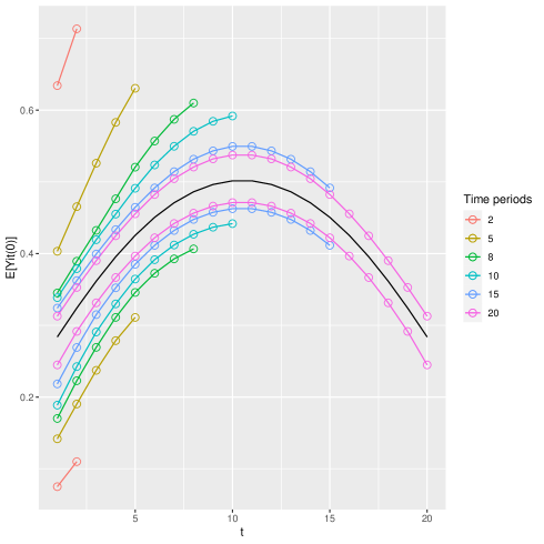
Figure 1: Bounds for the two-way binary choice probit model in Section 4.1 with varying number of time periods $T\leq 20$. The horizontal axis indicates the number of time periods $T$. The black solid curve indicates the true value of $\mathbb{E}\left[Y_{it}\left(0\right)\right]$. The colored curves are the upper and lower bounds from Theorem 2 using the first $t$ time periods, where $t$ is labeled in the legend.

Figure 2 presents results for the sequence $\mathbb{E}\left[Y_{it}\left(0\right)\right],t\geq 1$ for some variations on the model above. The first row, left column shows results for $T=8$, keeping the other design parameters unchanged. Note that, because $\lambda_{t}=\left(-1+2\frac{\left(t+1\right)}{T}\right)^{2}$, this changes the evolution of the expectation. All subpanels of Figure 2 display results for a deviation from the top left panel. All results in Figure 2 are for the sequence $\mathbb{E}\left[Y_{it}\left(0\right)\right],t\geq 1$, except for the top right panel, which shows the bounds for the sequence $\mathbb{E}\left[Y_{it}\left(1\right)\right],t\geq 1$, under the same model as that for the top left panel. The bounds are wider because $X_{it}$ has less mass around $1$ than around $0$. The second row reports bounds on the sequence $\mathbb{E}\left[Y_{it}\left(0\right)\right],t\geq 1$, when there are no time-effects (left column) and when there is no persistence in $X_{it}$, i.e. $\rho=0$ (right column). The bounds are slightly wider when the transformation function is time-invariant, and they are tighter when there is no persistence in $X_{i}$. The third row shows the bounds when $\sigma_{x}^{2}$ is $1/4$ (left column; compare to $\sigma_{x}^{2}=1$ in the benchmark case) and $\sigma_{x}^{2}=4$ (right column). The bounds when there is smaller cross-sectional variation in $X_{it}$ at a given time period $t$ are tighter than when there is greater cross-sectional variation.

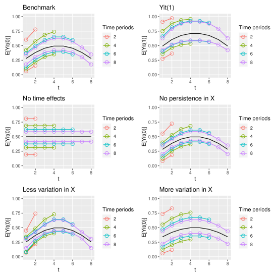
Figure 2: Bounds for the two-way binary choice probit model in Section 4.1, and variations, with varying number of time periods $T\leq 8$. All bounds are for $E\left[Y_{it}\left(0\right)\right]$, except for the top right panel, which shows bounds for $E\left[Y_{it}\left(1\right)\right]$. The black solid curve indicates the true value of the expectation, and the colored curves are the upper and lower bounds from Theorem 2 using the first $t$ time periods, where $t$ is labeled in the legend. See the main text for a description of the model for each panel.

For the specification consider in this section – binary probit with two way fixed-effects and short $T$ – there are no other results in the literature. In Appendix B, we present another numerical exercise for binary probit with discrete regressors. That DGP is the same as the one in Section 8 of Chernozhukov et al. (2013) when there are no time-effects, i.e. $\lambda_{t}=0$ for all $t$. In that case, we recover the bounds in Chernozhukov et al. (2013).

4.2 Staggered adoption with binary and ordered outcomes

In this section, we consider a staggered adoption design with both binary and $J$ ordered outcomes.

The population consists of $G$ groups and individuals in each group $g\in\left\{1,\cdots,G\right\}$ are observed over $T$ periods. Individuals are untreated up to and including period $g$; they are treated at period $g+1$, and then stay treated for $t>g+1$, i.e.

$$X_{it}=\begin{cases}0&\text{ if }t\leq g\left(i\right),\\ 1&\text{ if }t>g\left(i\right),\end{cases}$$

where $g\left(i\right)$ is individual $i$’s group. Here, $G=19$ and $T\in\left\{5,\dots,20\right\}$.

The latent outcome is given by

$$Y_{it}^{*} =\alpha_{i}+X_{it}\times 1-U_{it},$$

$$\alpha_{i} \sim\mathcal{N}\left(0,1\right)+\frac{g\left(i\right)}{G}-\frac{1}{2},$$

and $U_{it}$ is standard logistic. The observed outcome is generated as

$$Y_{it}\geq j\Leftrightarrow Y_{it}^{*}\geq\lambda_{jt},$$

where $j\in J\in\left\{2,4,6,8\right\}$, and the threshold $\lambda_{jt}$ is generated as follows. Set $\overline{J}\equiv\frac{J}{2}+1\in\left\{1,3,4,5\right\}$, so that $\left\{1,\cdots,\overline{J}-1\right\}$ are the lowest $J/2$ outcomes, and $\left\{\overline{J},\cdots,J\right\}$ are the top $J/2$ outcomes. Set $\lambda_{\overline{J}1}=0,\,\lambda_{\overline{J}t}\sim\mathcal{U}\left[-1,1\right]$, then draw $\eta_{+},\eta_{-}\sim\mathcal{U}\left[0,1\right]$ and construct

$$\lambda_{jt}=\begin{cases}\lambda_{\overline{J}t}-\frac{\left(\overline{J}-j\right)}{\overline{J}-1}\eta_{-},&\text{ if }j<\overline{J},\\ \lambda_{\overline{J}t}+\frac{\left(j-\overline{J}\right)}{\overline{J}-1}\eta_{+},&\text{ if }j>\overline{J},\end{cases}$$

We draw one set of $\left(\left(\lambda_{\overline{J}t}\right)_{t=2}^{T},\eta_{+},\eta_{-}\right)$ and condition our results on them. This allows us to compare the same parameter across different values of $J$ and $T$.

The parameter of interest is

$$\tau\equiv\mathbb{E}\left[\tau_{1,1,\overline{J}}\left(X_{i}\right)\right]=\mathbb{E}\left[P\left(\left.Y_{i1}\left(1\right)\geq\overline{J}\right|X_{i}\right)\right]=P\left(Y_{i1}\left(1\right)\geq\overline{J}\right),\,\overline{J}\in\left\{1,3,4,5\right\}.$$

This parameter gives the probability of being in the upper half of possible outcomes.

Our results for this design are presented in Figure 3. The solid black line is $\tau=P\left(Y_{i1}\left(1\right)\geq\overline{J}\right)$. Bounds for different values of $J$ are in colored, dashed lines. Binary choice is in red. At $T=5$, the width of the bounds for $\tau$ are approximately $0.35$, and become as narrow as $0.05$ when $T=20$. As $J$ increases, the bounds narrow substantially. This is especially evident when $T$ is small. For example, at $T=5$, the width of the bounds for $J=6$ is $0.07$, and for $J=8$ it is $0.02$.

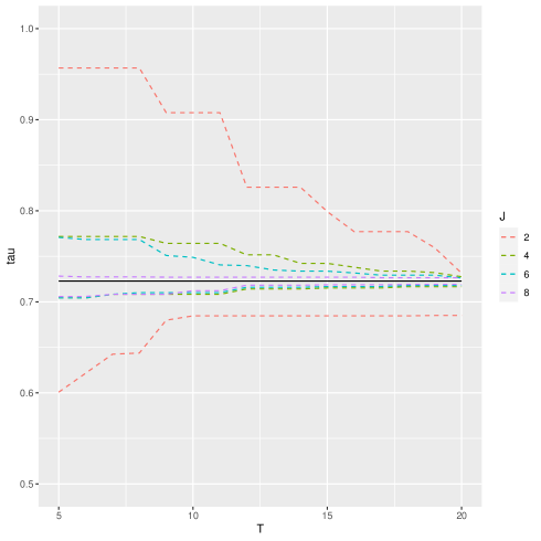
Figure 3: Results for staggered adoption with ordered outcomes. The solid black line is the true value of $\tau\equiv\mathbb{E}\left[\tau_{1,1,\overline{J}}\left(X_{i}\right)\right]$ (vertical axis). Each pair of dashed lines shows the bounds (vertical axis) as a function of the number of time periods used to construct the bound (horizontal axis). Colors indicate the number of support points for the ordered outcome variables, so that red corresponds to binary choice ($J=2$).

Figure 4 provides further insight, and further clarifies the construction of the bounds in Theorem 2. Consider $J=4$, $G=6$ and $T=8$. Each panel corresponds to a group $g\left(i\right)$, so that panel “3” corresponds to the population of individuals treated in periods $4-8$. The vertical error bars, at each $t$, correspond to the best bounds that can be constructed for the period-$1$ counterfactual using period-$t$ data, see Remark 6:

$$\left[\sup_{y^{\prime}\in\mathcal{Y}_{tL}}P\left(\left.Y_{is}\geq y^{\prime}\right|X_{i}\right),\inf_{y^{\prime}\in\mathcal{Y}_{tU}}P\left(\left.Y_{is}\geq y^{\prime}\right|X_{i}\right)\right]\cap\left[0,1\right],$$

with

$$\mathcal{Y}_{tL} \equiv\left\{y^{\prime}\in\mathcal{\underline{\mathcal{Y}}}:X_{is}\beta-h_{s}^{-}\left(y^{\prime}\right)\leq x\beta-h_{t}^{-}\left(y\right)\right\},$$

$$\mathcal{Y}_{tU} \equiv\left\{y^{\prime}\in\underline{\mathcal{Y}}:X_{is}\beta-h_{s}^{-}\left(y^{\prime}\right)\geq x\beta-h_{t}^{-}\left(y\right)\right\}.$$

From Figure 4, it is clear that $J=4$ is not sufficient to provide non-trivial bounds in each period, see for example periods 1-3. The bounds in period 4 are also trivial, but in a way that complements the period 1-3 bounds. Furthermore, the thresholds in periods 6-8 are such that these periods supply non-trivial bounds. By using Assumption 3, and taking the best bounds in each panel over the time periods as in Theorem 2, relatively narrow bounds are obtained on $\tau$, see Figure 3.

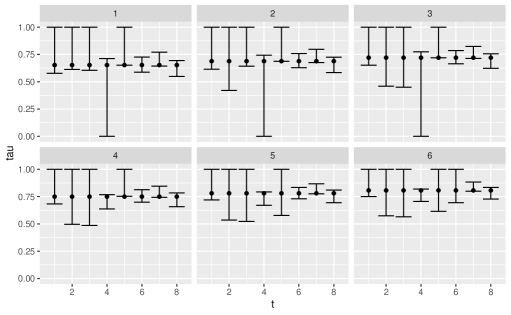
Figure 4: Details for the staggered adoption results with $J=4$ and $T=8$. The panels are numbered $g\in\left\{1,\cdots,6\right\}$. For each panel, $t$ on the horizontal axis is the time period from which the bound (error bar) is constructed for $P\left(\left.Y_{i1}\left(1\right)\geq 3\right|g\left(i\right)=g\right)$.

5 Conclusion

This paper discusses identification of counterfactual parameters in a class of nonlinear semiparametric panel models with fixed effects and arbitrary time effects. We derive bounds on the counterfactual survival probability and related functionals that depend on either outcomes from the same time period as the counterfactual (without exogeneity assumptions) or outcomes from across all available time periods (under a “strict exogeneity” or conditional time-stationarity assumption on the errors). The bounds tighten as the cardinality of the support of the dependent variable increases, and, under a time-stationarity assumption on the errors, as $T$ increases. The bounds need not collapse to a point as $T$ grows, rather they collapse to a point under particular assumptions on the time effects and the observed regressors, i.e. when the counterfactual index equals one of the observed indexes. Our bounds are valid for continuous and discrete outcomes and covariates, for both movers and stayers.

Although our focus is on identification, we describe here a potential way of addressing the issue of inference. Note that the bounds in Theorem 2 can be written as a set of conditional moment inequalities: for fixed $t,x,X_{i},y\in\underline{\mathcal{Y}}$ and for all $\left(s,y^{\prime}\in\underline{\mathcal{Y}}\right)$:

$$\mathbb{E}\left[\left.\left(X_{is}\beta-h_{s}^{-}\left(y^{\prime}\right)-\left(x\beta-h_{t}^{-}\left(y\right)\right)\right)\times\left(1\left\{Y_{is}\geq y^{\prime}\right\}-\tau_{t,x,y}\left(X_{i}\right)\right)\right|X_{i}\right]\geq 0.$$

When $\left(\beta,h_{t}\right)$ are partially identified via a set of moment inequalities, these moment inequalities can be added to the program. For either pointwise or uniform in $x$ inference, one could implement the full vector approach of Cox and Shi (2022) if the regressors have finite support, or Andrews and Shi (2017) if the regressors are continuously distributed.

The bounds of Theorem 1 are valid for dynamic panel models. However, the bounds may be wider than those obtained by studying specific models, where the dynamic structure is known, e.g., binary choice with lagged outcomes as covariates. In ongoing work, we are studying how to extend our approach to such models. It is an open question as to whether our approach could be extended to nonseparable models.

Appendix A Proofs

Proof of Theorem 1..

Define the (potential) latent variables

$$Y_{it}^{*}\left(x\right) \equiv\alpha_{i}+x\beta-U_{it},$$ (19)

$$Y_{it}^{*} \equiv Y_{it}^{*}\left(X_{it}\right).$$

Assumption 2 obtains the following equivalent relationships:

$$Y_{it}\left(x\right)\geq y$$

$$\Leftrightarrow Y_{it}^{*}\left(x\right)\geq h_{t}^{-}\left(y\right)$$ (20)

$$\Leftrightarrow U_{it}-\alpha_{i}\leq x\beta-h_{t}^{-}\left(y\right),$$ (21)

that is, the counterfactual outcome being greater than a fixed value $y$ is equivalent to the random variable $U_{it}-\alpha_{i}$ being smaller than the counterfactual index evaluated at $y$.

Then, for any value $y^{\prime}\in\mathcal{Y}$, the following are equivalent:

$$X_{it}\beta-h_{t}^{-}\left(y^{\prime}\right)\geq x\beta-h_{t}^{-}\left(y\right)$$

$$\Leftrightarrow$$

$$P\left(\left.Y_{it}\geq y^{\prime}\right|X_{i}\right)\geq P\left(\left.Y_{it}\left(x\right)\geq y\right|X_{i}\right)=\tau_{t,x,y}\left(X_{i}\right).$$

To see this, suppose that there exists a $y^{\prime}$ such that

$$X_{it}\beta-h_{t}^{-}\left(y^{\prime}\right)\geq x\beta-h_{t}^{-}\left(y\right).$$

Then:

$$P\left(\left.Y_{it}\geq y^{\prime}\right|X_{i}\right) =P\left(\left.Y_{it}^{*}\geq h_{t}^{-}\left(y^{\prime}\right)\right|X_{i}\right)$$

$$=P\left(\left.\alpha_{i}+X_{it}\beta-U_{it}\geq h_{t}^{-}\left(y^{\prime}\right)\right|X_{i}\right)$$

$$=P\left(\left.U_{it}-\alpha_{i}\leq X_{it}\beta-h_{t}^{-}\left(y^{\prime}\right)\right|X_{i}\right)$$

$$\geq P\left(\left.U_{it}-\alpha_{i}\leq x\beta-h_{t}^{-}\left(y\right)\right|X_{i}\right)$$

$$=P\left(\left.\alpha_{i}+x\beta-U_{it}\geq h_{t}^{-}\left(y\right)\right|X_{i}\right)$$

$$=P\left(\left.Y_{it}\left(x\right)\geq y\right|X_{i}\right)$$

$$=\tau_{t,x,y}\left(X_{i}\right),$$

where the inequality follows by weak monotonicity of CDFs. ∎

Proof of Theorem 2.

Chernozhukov et al. 2015 point out that Assumption 3 is equivalent to $\left.\alpha_{i},U_{it}\right|X_{i}\stackrel{{\scriptstyle d}}{{=}}\left.\alpha_{i},U_{i1}\right|X_{i}$. In particular,

$$\left.U_{it}-\alpha_{i}\right|X_{i}\stackrel{{\scriptstyle d}}{{=}}\left.U_{is}-\alpha_{i}\right|X_{i},\,s,t\in\left\{1,\dots,T\right\}.$$ (22)

Then, for any $\left(x,X_{i},t,y,s,y^{\prime}\right)$ we have that

$$X_{is}\beta-h_{s}^{-}\left(y^{\prime}\right)\geq x\beta-h_{t}^{-}\left(y\right)$$

$$\Leftrightarrow$$

$$P\left(\left.Y_{is}\geq y^{\prime}\right|X_{i}\right)\geq P\left(\left.Y_{it}\left(x\right)\geq y\right|X_{i}\right)=\tau_{t,x,y}\left(X_{i}\right).$$

This follows from

$$P\left(\left.Y_{is}\geq y^{\prime}\right|X_{i}\right) =P\left(\left.Y_{is}^{*}\geq h_{s}^{-}\left(y^{\prime}\right)\right|X_{i}\right)$$

$$=P\left(\left.\alpha_{i}+X_{is}\beta-U_{is}\geq h_{s}^{-}\left(y^{\prime}\right)\right|X_{i}\right)$$

$$=P\left(\left.U_{is}-\alpha_{i}\leq X_{is}\beta-h_{s}^{-}\left(y^{\prime}\right)\right|X_{i}\right)$$

$$=P\left(\left.U_{it}-\alpha_{i}\leq X_{is}\beta-h_{s}^{-}\left(y^{\prime}\right)\right|X_{i}\right)$$

$$\geq P\left(\left.U_{it}-\alpha_{i}\leq x\beta-h_{t}^{-}\left(y\right)\right|X_{i}\right)$$

$$=P\left(\left.\alpha_{i}+x\beta-U_{it}\geq h_{t}^{-}\left(y\right)\right|X_{i}\right)$$

$$=P\left(\left.Y_{it}\left(x\right)\geq y\right|X_{i}\right)$$

$$=\tau_{t,x,y}\left(X_{i}\right).$$

The argument is similar to that in the proof of Theorem 1, except that the fourth equality follows by (22), and the fifth inequality follows by weak monotonicity of CDFs. ∎

Appendix B Numerical experiment with discrete regressors

We consider here a numerical exercise inspired by Section 8 in Chernozhukov et al. (2013): a probit model with discrete regressors. When the structural equation is time-invariant, the data generating process corresponds to that in Chernozhukov et al. (2013). We present results for, first, the time-invariant case – for which our bounds correspond to those in Chernozhukov et al. (2013), and then for a time-varying case.

The data generating process is:

$$Y_{it} =1\left\{\alpha_{i}+X_{it}\beta-U_{it}-\lambda_{t}\geq 0\right\},\,t=1,2,$$ (23)

$$\alpha_{i} \sim\mathcal{N}\left(0,1\right),$$

$$U_{it} \sim\mathcal{N}\left(0,1\right),$$

$$\eta_{it} \sim\mathcal{N}\left(0,1\right),\,t=1,2,$$

$$X_{it} =1\left\{\alpha_{i}\geq\eta_{it}\right\},\,t=1,2,$$

$$\lambda_{1} =0,$$

$$\lambda_{2} \in\left\{0,\frac{1}{2},1\right\},$$

$$\beta \in\left[0,2\right].$$

We consider the ATE at $t=1,2$, defined as:

$$ATE_{t} \equiv\mathbb{E}_{X}\left(P\left(\left.Y_{it}\left(1\right)\geq 1\right|X_{i}\right)-P\left(\left.Y_{it}\left(0\right)\geq 1\right|X_{i}\right)\right)$$

$$=\mathbb{E}_{X}\left(\tau_{t,1,1}\left(X_{i}\right)-\tau_{t,0,1}\left(X_{i}\right)\right).$$

Recall that $\tau_{t,0,1}\left(X_{i}\right)$ refers to the counterfactual probability that in period $t$ (first index), the probability that the counterfactual outcome under $x=0$ (second index) for the the subpopulation with $X_{i}$ equals or exceeds $y=1$ (third index). For simplicity, we set $t=1$, so that the counterfactual index for the analysis that follows is:

$$x\beta-\lambda_{1}=0.$$ (24)

According to Theorem 2, if the observed index is smaller (greater) than the counterfactual index (24), the observed probability associated with the observed index provides a lower (upper) bound on the counterfactual probability, while if the observed index equals the counterfactual index, the observed probability point identifies the counterfactual probability.

First, in order to compare our results to those in Chernozhukov et al. (2013), we set $\lambda_{2}=0$. Theorem 2 then obtains the following results for $\tau_{1,0,1}\left(X_{i}\right)$ and $\tau_{1,1,1}\left(X_{i}\right)$. Note that $\tau_{1,0,1}\left(X_{i}\right)$ is point-identified for the subpopulations with

$$X_{i}\in\left\{\left(0,0\right),\left(0,1\right),\left(1,0\right)\right\},$$

because for the listed subpopulations, the value $x=0$ is observed in at least one of the periods. Thus:

$$\tau_{1,0,1}\left(\left(0,0\right)\right) =P\left(\left.Y_{i1}\geq 1\right|X_{i}=\left(0,0\right)\right)=P\left(\left.Y_{i2}\geq 1\right|X_{i}=\left(0,0\right)\right),$$

$$\tau_{1,0,1}\left(\left(0,1\right)\right) =P\left(\left.Y_{i1}\geq 1\right|X_{i}=\left(0,1\right)\right),$$

$$\tau_{1,0,1}\left(\left(1,0\right)\right) =P\left(\left.Y_{i2}\geq 1\right|X_{i}=\left(1,0\right)\right).$$

For the subpopulation of stayers with $X_{i}=\left(1,1\right)$, the value $x=0$ is not observed in either time period, so the counterfactual probability $\tau_{1,0,1}\left(\left(1,1\right)\right)$ is partially identified unless $\beta=0$:

$$\tau_{1,0,1}\left(\left(1,1\right)\right)\in\begin{cases}\left[0,P\left(\left.Y_{i1}\geq 1\right|X_{i}=\left(1,1\right)\right)\right],&\beta>0,\\ \left[P\left(\left.Y_{i1}\geq 1\right|X_{i}=\left(1,1\right)\right),1\right],&\beta<0,\\ \left\{P\left(\left.Y_{i1}\geq 1\right|X_{i}=\left(1,1\right)\right)\right\}.&\beta=0.\end{cases}$$

This is because the observed index for this subpopulation is $\beta$ in both time periods.

The analysis for $\tau_{1,1,1}\left(X_{i}\right)$ is similar and omitted. Figure 5 plots the bounds for $ATE_{t=1}$. Note that our bounds for this particular example coincide with those in Chernozhukov et al. (2013) that the authors call “NPM.”

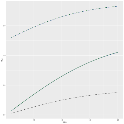
Figure 5: Bounds for binary choice probit model with discrete regressors and no time effects in (23). The solid line shows the true ATE at $t=1$ on the vertical axis, with the true value of $\beta$ on the horizontal axis. The dotted lines show the upper and lower bounds from Theorem 2, described in the main text of Appendix B.

Consider now the specification with positive time effects, $\lambda_{2}>0$. Theorem 2 then obtains the following results for $\tau_{1,0,1}\left(X_{i}\right)$ and $\tau_{1,1,1}\left(X_{i}\right)$.

First, $\tau_{1,0,1}\left(X_{i}\right)$ is point-identified for the subpopulations with $X_{i1}=0$: the stayers with $X_{i}=\left(0,0\right)$ and the movers with $X_{i}=\left(0,1\right)$. This is because $x=0$ at $t=1$ for those subpopulations, so that the observed index for these subpopulations equals the counterfactual index. Thus,

$$\tau_{1,0,1}\left(\left(0,0\right)\right) =P\left(\left.Y_{i1}\geq 1\right|X_{i}=\left(0,0\right)\right),$$

$$\tau_{1,0,1}\left(\left(0,1\right)\right) =P\left(\left.Y_{i1}\geq 1\right|X_{i}=\left(0,1\right)\right).$$

Second, for the subpopulation of movers with $X_{i}=\left(1,0\right)$, the period $t=2$ observed probability provides a lower bound on $\tau_{1,0,1}\left(X_{i}\right)$ because the observed index for this subpopulation is $X_{i2}\beta-\lambda_{2}=-\lambda_{2}$, which is smaller than the counterfactual index since we assumed that $\lambda_{2}>0$, so:

$$\tau_{1,0,1}\left(\left(1,0\right)\right)\geq P\left(\left.Y_{i2}\geq 1\right|\left(1,0\right)\right).$$

Whether the $t=1$ observed probabilities point or partially identify $\tau_{1,0,1}\left(\left(1,0\right)\right)$ for this subpopulation depends on how the observed index $X_{i1}\beta-\lambda_{1}=\beta$ compares to the counterfactual index in (24):

$$\tau_{1,0,1}\left(\left(1,0\right)\right) =P\left(\left.Y_{i1}\geq\right|\left(1,0\right)\right),\text{ if }\beta=0,$$

$$\tau_{1,0,1}\left(\left(1,0\right)\right) <P\left(\left.Y_{i1}\geq\right|\left(1,0\right)\right),\text{ if }\beta>0,$$

$$\tau_{1,0,1}\left(\left(1,0\right)\right) >P\left(\left.Y_{i1}\geq\right|\left(1,0\right)\right),\text{ if }\beta<0.$$

Third, for the subpopulation of stayers with $X_{i}=\left(1,1\right)$, the observed index at $t=1$ is $X_{i1}\beta-\lambda_{1}=\beta$, so that comparing it to the counterfactual index in (24) obtains:

$$\tau_{1,0,1}\left(\left(1,1\right)\right) =P\left(\left.Y_{i1}\geq\right|\left(1,1\right)\right),\text{ if }\beta=0,$$

$$\tau_{1,0,1}\left(\left(1,1\right)\right) <P\left(\left.Y_{i1}\geq\right|\left(1,1\right)\right),\text{ if }\beta>0,$$

$$\tau_{1,0,1}\left(\left(1,1\right)\right) >P\left(\left.Y_{i1}\geq\right|\left(1,1\right)\right),\text{ if }\beta<0,$$

while the observed index at $t=2$ for this subpopulation is $X_{i2}\beta-\lambda_{2}=\beta-\lambda_{2}$, which compared to the same counterfactual index in (24) obtains:

$$\tau_{1,0,1}\left(\left(1,1\right)\right) =P\left(\left.Y_{i2}\geq\right|\left(1,1\right)\right),\text{ if }\beta=\lambda_{2},$$

$$\tau_{1,0,1}\left(\left(1,1\right)\right) >P\left(\left.Y_{i2}\geq\right|\left(1,1\right)\right),\text{ if }\beta<\lambda_{2},$$

$$\tau_{1,0,1}\left(\left(1,1\right)\right) <P\left(\left.Y_{i2}\geq\right|\left(1,1\right)\right),\text{ if }\beta>\lambda_{2}.$$

We have now described all the restrictions underlying Theorem 2 for $\tau_{1,0,1}\left(X_{i}\right)$ for all $X_{i}$ in our example. The bounds now follow by selecting the best bounds for each case and for each $X_{i}$ as in Theorem 2. The same analysis can be done for $\tau_{1,1,1}\left(X_{i}\right)$ and for period 2 counterfactuals.

Figure 6 plots the bounds for ATE_t=1 (left panel) and ATE_t=2 (right panel). The solid lines correspond to the true ATEs, while the dashed lines correspond to their respective bounds, grouped by color. The colors correspond to different values of $\lambda_{2}$. For example, in both panels, the red lines correspond to the true ATE and its bounds when $\lambda_{2}=0$ (no time-effects). In the left panel, all true ATEs have the same value since there are no time-effects, $\lambda_{1}=0$, while in the right panel the true ATEs have different values because they correspond to different time effects.

Figure 6: Bounds for the ATE for a probit model with discrete regressors and time effects at different time periods. The solid lines show the true ATE at time 1 (left panel) and time 2 (right panel), while the dotted lines show the bounds on the ATEs. The colors correspond to the three different values of $\lambda_{2}.$ The dotted lines corresponding to $\lambda_{2}=0$ in the left panel correspond to the bounds for the binary probit model without time effects and with discrete regressors as in Chernozhukov et al. (2013). The bounds corresponding to $\lambda_{2}\neq 0$ correspond to the bounds for the binary probit with time effects and discrete regressors computed via Theorem 2.

References

• Abrevaya (1999) Abrevaya, J. (1999). Leapfrog Estimation of a Fixed-Effects Model with Unknown Transformation of the Dependent Variable. Journal of Econometrics 93, 203–228.
• Abrevaya (2000) Abrevaya, J. (2000). Rank Estimation of a Generalized Fixed-Effects Regression Model. Journal of Econometrics 95(1), 1–23.
• Abrevaya and Muris (2020) Abrevaya, J. and C. Muris (2020). Interval Censored Regression with Fixed Effects. Journal of Applied Econometrics 35(2), 198–216.
• Aguirregabiria and Carro (2021) Aguirregabiria, V. and J. M. Carro (2021). Identification of Average Marginal Effects in Fixed Effects Dynamic Discrete Choice Models. Technical report. Available at https://doi.org/10.48550/arXiv.2107.06141.
• Ahn et al. (2018) Ahn, H., H. Ichimura, J. Powell, and P. Ruud (2018). Simple Estimators for Invertible Index Models. Journal of Business and Economic Statistics 36(1), 1–10.
• Altonji and Matzkin (2005) Altonji, J. G. and R. L. Matzkin (2005). Cross Section and Panel Data Estimators for Nonseparable Models with Endogenous Regressors. Econometrica 73(4), 1053–1102.
• Amemiya and Powell (1981) Amemiya, T. and J. L. Powell (1981, December). A comparison of the Box-Cox maximum likelihood estimator and the non-linear two-stage least squares estimator. Journal of Econometrics 17(3), 351–381.
• Andrews and Shi (2017) Andrews, D. and X. Shi (2017). Inference Based on Many Conditional Moment Inequalities. Journal of Econometrics 196, 274–287.
• Arellano and Bonhomme (2011) Arellano, M. and S. Bonhomme (2011). Nonlinear Panel Data Analysis. Annual Review of Economics 3, 395–424.
• Arellano and Carrasco (2003) Arellano, M. and R. Carrasco (2003). Binary Choice Panel Data Models with Predetermined Variables. Journal of Econometrics 115, 125–157.
• Arellano and Honoré (2001) Arellano, M. and Honoré (2001). Panel Data Models: Some Recent Developments. Handbook of econometrics, Volume 5, 3229–3296.
• Aristodemou (2021) Aristodemou, E. (2021). Semiparametric Identification in Panel Data Discrete Response Models. Journal of Econometrics 220(2), 253–271.
• Athey and Imbens (2006) Athey, S. and G. W. Imbens (2006). Identification and Inference in Nonlinear Difference-in-Differences Model. Econometrica 74(2), 431–497.
• Baetschmann (2012a) Baetschmann, G. (2012a). Identification and Estimation of Thresholds in the Fixed Effects Ordered Logit Model. Economics Letters 115(3), 416–418.
• Baetschmann (2012b) Baetschmann, G. (2012b). Identification and Estimation of Thresholds in the Fixed Effects Ordered Logit Model. Economics Letters 115(3), 416–418.
• Bartolucci et al. (2023) Bartolucci, F., C. Pigini, and F. Valentini (2023). Conditional inference and bias reduction for partial effects estimation of fixed-effects logit models. Empirical Economics 64, 2257–2290.
• Bester and Hansen (2009) Bester, C. A. and C. B. Hansen (2009). Identification of Marginal Effects in a Nonparametric Correlated Random Effects Model. Journal of Business and Economic Statistics 27(2), 235–250.
• Blundell and Powell (2003) Blundell, R. W. and J. L. Powell (2003). Endogeneity in Nonparametric and Semiparametric Regression Models. In M. Dewatripont, L. Hansen, and S. Turnovsky (Eds.), Advances in Economics and Econometrics: Theory and Applications, Volume Eighth World Congress, Vol. II. Oxford: Cambridge University Press.
• Blundell and Powell (2004) Blundell, R. W. and J. L. Powell (2004). Endogeneity in Semiparametric Binary Response Models. Review of Economic Studies 71(3), 655–679.
• Bonhomme (2012) Bonhomme, S. (2012). Functional Differencing. Econometrica 80(4), 1337–1385.
• Botosaru and Muris (2017) Botosaru, I. and C. Muris (2017). Binarization for Panel Models with Fixed Effects. Technical report. cemmap Working paper CWP31/17, available at https://www.cemmap.ac.uk/publication/binarization-for-panel-models-with-fixed-effects/.
• Botosaru et al. (2021) Botosaru, I., C. Muris, and K. Pendakur (2021). Identification of Time-Varying Transformation Models with Fixed Effects, with an Application to Unobserved Heterogeneity in Resource Shares. Journal of Econometrics.
• Botosaru et al. (2022) Botosaru, I., C. Muris, and S. Sokullu (2022). Partial Effects in Time-Varying Linear Transformation Panel Models with Endogeneity. Technical report. University of Bristol, School of Economics Discussion Paper 22/756.
• Chamberlain (1984) Chamberlain, G. (1984). Panel Data. In Z. Griliches and M. Intriligator (Eds.), Handbook of Econometrics, Volume 2, Chapter 22, pp.  1247–1315. Elsevier.
• Charlier et al. (2000) Charlier, E., B. Melenberg, and A. van Soest (2000). Estimation of a Censored Regression Panel Data Model Using Conditional Moment Restrictions Efficiently. Journal of Econometrics 95(1), 25–56.
• Chen (2010) Chen, S. (2010). An Integrated Maximum Score Estimator for a Generalized Censored Quantile Regression Model. Journal of Econometrics 155(1), 90–98.
• Chen et al. (2005) Chen, S., G. Dahl, and S. Khan (2005). Nonparametric Identification and Estimation of a Censored Location-Scale Regression Model. Journal of the American Statistical Association 100(469), 212–221.
• Chen et al. (2019) Chen, S., S. Khan, and X. Tang (2019). Exclusion Restrictions in Dynamic Binary Choice Panel Data Models: Comment on Semiparametric Binary Choice Panel Data Models Without Strictly Exogenous Regressors. Econometrica 87, 1781–1785.
• Chen et al. (2022) Chen, S., X. Lu, and X. Wang (2022). Nonparametric Estimation of Generalized Transformation Models with Fixed Effects. Econometric Theory, 1–32.
• Chen and Wang (2018) Chen, S. and X. Wang (2018). Semiparametric Estimation of Panel Data Models without Monotonicity or Separability. Journal of Econometrics 206, 515–530.
• Chernozhukov et al. (2013) Chernozhukov, V., I. Fernández-Val, J. Hahn, and W. K. Newey (2013). Average and Quantile Effects in Nonseparable Panel Models. Econometrica 81(2), 535–580.