The Multi-Armed Bandit Problem Under the Mean-Variance Setting

Abstract

The classical multi-armed bandit problem involves a learner and a collection of arms, with unknown reward distributions. At each round, the learner selects an arm and receives new information. The learner faces a tradeoff between exploiting the current information and exploring all arms. The objective is to maximize the expected cumulative reward over all rounds. Such an objective does not involve a risk-reward tradeoff, which is fundamental in many areas of application. In this paper, we build upon Sani et al. (2012)’s extension of the classical problem to a mean-variance setting. We relax their assumptions of independent arms and bounded rewards, and we consider sub-Gaussian arms. We introduce the Risk-Aware Lower Confidence Bound algorithm to solve the problem, and study some of its properties. We perform numerical simulations to demonstrate that, in both independent and dependent scenarios, our approach performs better than the algorithm suggested by Sani et al. (2012)

Keywords: applied probability, multiarmed bandits, mean-variance regret analysis, sub-Gaussian distribution, online optimization

1 Introduction

The multi-armed bandit (MAB) problem is a type of online learning and sequential decision-making problem. A classical MAB problem involves $K$ independent arms, each with its own independent reward distribution, and a learner. In the problem, each arm generates a random reward from the underlying probability distribution, which is unknown in advance. At each round, the learner selects one arm among $K$ arms and receives a new observation from that arm. The learner often faces a tradeoff between exploiting the current information and exploring all arms. Given a finite number of $n$ rounds, the design objective aims to maximize the cumulative reward over $n$ rounds.

The MAB framework has been applied to a wide range of real-world problems, including clinical trials (Durand et al. (2018)), recommendation systems (Mary et al. (2015)), telecommunication (Boldrini et al. (2018)) and finance (Shen et al. (2015)). For example, in finance (Shen et al. (2015)), the actions correspond to the proposed portfolio composition, and the reward represents the performance of the proposed portfolio. The exploration–exploitation dilemma in the above example is whether to try a new portfolio composition or keep using the current portfolio with the best historical performance.

As is standard in the literature, we measure the welfare implications of a given selection policy by the notion of regret. The latter is defined as the difference between the expected cumulative rewards under the true distribution and the empirical distribution.

1.1 Related Work

The MAB problem has been explored by Thompson (1933) and Robbins (1952) as a useful tool for constructing online sequential decision algorithms. Thompson (1933) proposed a Bayes-optimal approach that directly maximizes expected cumulative rewards with respect to a given prior distribution. Robbins (1952) first formalized the classic MAB problem, in which each arm follows an unknown distribution over [0,1], and rewards are independent draws from the distribution corresponding to the chosen arm. Since then, a number of methods have been developed to solve the MAB problem. Most of the possible ways to solve the MAB problem can be defined into three categories:

• $\epsilon$-greedy algorithm: is a straightforward method for balancing exploration and exploitation by employing a greedy policy to take action with a probability of $1-\epsilon$, and a random action with a small probability of $\epsilon$.

• Upper confidence bounds (UCB) algorithm: is often phrased as “optimism in the face of uncertainty”. The algorithm uses the observed data so far to assign a value (i.e., upper confidence bound index) to each arm, where the arm with the higher index value will be selected with a higher probability in the next round. Strong theoretical guarantees on the rate of regret can be attained by implementing the UCB algorithm. Early work on using UCB to solve MAB problems was done by Lai and Robbins (1985), Agrawal (1995) and Auer et al. (2002). The technique of upper confidence bounds (UCB) for the asymptotic analysis of regret was introduced by Lai and Robbins (1985), who demonstrated that the minimum regret has a logarithmic order in $n$. As a simpler formulation, Agrawal (1995) discusses the MAB problem under a finite-time setting. Auer et al. (2002) conduct a finite-time analysis of the classic MAB with bounded rewards using the UCB algorithm.

• Thompson sampling: is the first algorithm for the bandit problem proposed by Thompson (1933). Thompson sampling has a simple idea. By implementing Thompson sampling, the learner selects a prior over a set of possible bandit environments at the start. In each round, the learner makes an action chosen randomly from the posterior. Thompson Sampling has been empirically proved to be effective by Chapelle and Li (2011). In comparison to the UCB algorithm, Thompson Sampling does not have strong theoretical guarantees on regret. May et al. (2012) and Agrawal and Goyal (2012) conducted theoretical analysis and established weak guarantees on regret.

In the classic MAB formulation, the learner maximizes the expected cumulative reward within a finite time frame. Nevertheless, in real practice, maximizing the expected reward may not be the ultimate goal. For instance, in portfolio selection, the portfolio that performs best during a period of the economic boom may lead to a substantial loss when the economy is struggling. In clinical trials, the treatment that works best on average may result in side effects for some patients. In many cases, a learner’s primary goal may be to effectively balance risk and return. There is no universally accepted definition of risk. Among various risk modelling paradigms, the mean-variance paradigm (Markowitz (1968)) and the expected utility theory (Morgenstern and Von Neumann (1953)) are the two fundamental risk modelling paradigms.

The work of Sani et al. (2012), in which the criteria of mean-variance of data was first introduced, is the most important reference to our study. Sani et al. (2012) study the problem where each arm’s distribution is bounded, and the learner’s objective is to minimize the mean-variance of rewards collected over a finite time. Their proposed Mean-Variance Lower Confidence Bound (MVLCB) algorithm achieves a learning regret of $\mathcal{O}(\log^{2}(n))$. As an improvement, Vakili and Zhao (2016) analyze the problem under the mean-variance setting, but with the assumption that the square of the underlying $X$ is sub-Gaussian. Vakili and Zhao (2016)’s algorithm achieves a learning regret of $\mathcal{O}(\log(n))$. Furthermore, Vakili and Zhao (2015) extend the previous setup by taking into account the value-at-risk (VaR) of total rewards over a finite time horizon and ending with a learning regret of $\mathcal{O}(f(n)\log(n))$, where $f(n)$ is a positive increasing diverging sequence. Zhu and Tan (2020) examine the possibilities of Thompson sampling methods for solving mean-variance MAB and provide a detailed regret analysis for Gaussian and Bernoulli bandits with comparable learning regret $\mathcal{O}(\log(n))$. In addition, they run a large number of simulations to compare their algorithms against existing UCB-based methods for different risk tolerances. As another way of measuring the risk, conditional-value-at-risk (CVaR) has been studied in solving risk-averse MAB by Galichet et al. (2014), Kagrecha et al. (2019) and Prashanth et al. (2020). Galichet et al. (2014) show that their proposed algorithm’s learning regret under the CVaR scheme is $\mathcal{O}(\log(n))$. As a follow-up, Kagrecha et al. (2019) conduct a theoretical study of CVaR-based algorithm for MAB with unbounded rewards, and Prashanth et al. (2020) compare the performance of CVaR-based algorithm under light-tailed and heavy-tailed distributions.

Both Sani et al. (2012) and Galichet et al. (2014) study the risk-aware MAB problem by assuming independent bounded arms. Such an assumption limits the application of their results. In real-life problems, multiple arms may expose the same source of risk, and the distribution of each arm may not necessarily be bounded. As a pioneer, Liu et al. (2021) create a risk-aware UCB algorithm for Gaussian distributions that has a learning regret of $\mathcal{O}(\log(n))$. The Thompson sampling methods are then used by Gupta et al. (2021) to analyze the correlated bandit problems, where the underlying distributions are bounded. They categorize the arms as competitive or non-competitive, assuming that correlations between the arms arise from a latent random source. For the competitive group, their algorithm produces a learning regret of $\mathcal{O}(\log(n))$, whereas for the non-competitive group, it can only produce $\mathcal{O}(1)$.

Bandit learning algorithms are now widely used in a variety of fields. However, the application of bandit learning to finance has received little attention from researchers due to the inherent difference between financial assets and classic bandits.

• Independence: the classic MAB problem assumes i.i.d. reward distributions for each arm, which does not apply to financial asset returns. Assets are correlated in the financial markets, and the performance of one asset can reveal important information about the other assets. A lower regret bound can be obtained by exploiting the dependence; for example, Gupta et al. (2021) pioneered the analysis of the correlated MAB problem.

• Single pull: the classic MAB problem only allows one arm to be pulled at each round, while portfolio selection strategies often result in a basket of financial assets for investment.

• Risk-return balance: the classic MAB problem is only concerned with maximizing mean reward, while good portfolio selection strategies focus on risk-adjusted return (i.e., Sharpe ratio, mean-variance).

• Historical data: the classic MAB problem has no historical data, whereas sufficient historical data is available for publicly traded financial assets.

Shen et al. (2015) use a principal component decomposition (PCA) to construct an orthogonal portfolio from correlated assets, and they derive the optimal portfolio strategy using the UCB framework based on risk-adjusted reward. Later, Shen et al. (2015) treat classic portfolio strategies in finance as strategic arms, and they leverage the Thompson sampling method to mix two different strategic arms.

1.2 Contributions

In this paper, we analyze the risk-aware MAB problem under a mean-variance setting. Under this setting, we relax the assumptions about the underlying distribution of each arm. We allow each arm to be correlated, and the distributions of the arms belong to the sub-Gaussian distribution class. We introduce the Risk Aware Lower Confidence Bound (RALCB) algorithm, a member of the extensive family of Lower Confidence Bound algorithms. Additionally, we give a theoretical analysis of the algorithms and obtain the upper bounds on the expected regret for the suggested algorithm. Finally, we perform a number of numerical simulations to demonstrate that, in both independent and dependent scenarios, our suggested approach performs better than the MVLCB suggested by Sani et al. (2012).

The rest of this paper is organized as follows: In Section 2, we introduce the MAB problem under the mean-variance setting. In Section 3, the confidence-bound algorithm is introduced, and its theoretical characteristics are examined in Section 3.1. A possible extension of MAB problems is examined in Section 3.2. The theoretical findings are then supported by a set of numerical simulations in Section 4 and the proposed algorithm is applied to solve the financial investment problem in Section 4.7. Results of supporting proofs are provided in Section 5.

2 Problem Formulation

In this section, we introduce notation and define the risk-aware MAB problem. The classic $K$-armed bandit problem has a finite action set $\mathcal{A}\mathrel{\mathop{\mathchar 58\relax}}=\{1,...,K\}$. The learner interacts with the environment sequentially over time. Let $\{X^{i}_{t}\mathrel{\mathop{\mathchar 58\relax}}i=1,...,K,t=1,2,...\}$ denote the real-valued rewards from pulling arm $i\in\{1,...,K\}$ at time $t\in\{1,2,...\}$. The $X^{i}_{t}$ are modeled as random variables on a given probability space $(\Omega,\mathcal{F},\mathbb{P})$. We assume that each $X^{i}_{t}$ belongs to the class of sub-Gaussian random variables. Recall that a random variable $X$ is called sub-Gaussian if there is a constant $\theta\geq 0$ such that for all $a\in\mathbb{R}$:

$$\mathbb{E}_{\mathbb{P}}[e^{a(X-\mathbb{E}_{\mathbb{P}}[X])}]\leq e^{\frac{a^{2}\theta^{2}}{2}}.$$

Clearly, all Gaussian random variables are also sub-Gaussian. According to Hoeffding’s lemma in Hoeffding (1963), all bounded random variables are sub-Gaussian. We refer to Wainwright (2019) for a discussion of the mathematical properties of sub-Gaussian random variables.

We assume that the random vectors $\textbf{X}_{t}\mathrel{\mathop{\mathchar 58\relax}}=(X^{1}_{t},X^{2}_{t},...,X^{K}_{t})$ are independent and identically distributed (i.i.d.). A policy $\pi_{t}$ that the learner follows is a random variable taking values in $\{1,\dots,K\}$, depending only on $(X^{\pi_{1}}_{1},\dots,X^{\pi_{t-1}}_{t-1},\pi_{1},\dots,\pi_{t-1})$. In each round $t$, the learner selects an arm $\pi_{t}\in\mathcal{A}$ based on information available at $t$. The environment then samples a reward $X^{\pi_{t}}_{t}$ and reveals it to the learner. As a result, the learner is unable to make decisions based on future observations.

In the classic MAB problem, the goal of the learner is to maximize the expected cumulative rewards. In this paper, we also take the risk into consideration. To effectively balance the expected reward and the risk, we use the same mean-variance setting as in Sani et al. (2012). Let the coefficient of absolute risk tolerance $\rho\geq 0$ be given and fixed, and define for every arm $i$,

$$\textup{MV}^{\rho}_{i}\mathrel{\mathop{\mathchar 58\relax}}=\sigma_{i}^{2}-\rho\mu_{i},$$

where $\mu_{i}$ and $\sigma_{i}^{2}$ denote the mean and variance of $X_{i}$. The optimal arms are defined as $i^{\rho}_{0}\in\mathop{\rm arg\,min}_{i\in\mathcal{A}}\textup{MV}^{\rho}_{i}$.

Given a learning policy $\pi_{t}$ and a reward process $\left\{X^{\pi_{t}}_{t}\right\}^{n}_{t=1}$, the empirical mean-variance of the learning policy can be defined as

$$\widehat{\textup{MV}}^{\rho}(\pi)\mathrel{\mathop{\mathchar 58\relax}}=\hat{\sigma}^{2}(\pi)-\rho\hat{\mu}(\pi),$$ (1)

where

$$\hat{\mu}(\pi)\mathrel{\mathop{\mathchar 58\relax}}=\frac{1}{n}\sum_{t=1}^{n}X^{\pi_{t}}_{t},\;\;\;\;\;\hat{\sigma}^{2}(\pi)\mathrel{\mathop{\mathchar 58\relax}}=\frac{1}{n}\sum_{t=1}^{n}(X^{\pi_{t}}_{t}-\hat{\mu}(\pi))^{2}.$$ (2)

The objective of the risk-aware MAB problem is to minimize $\widehat{\textup{MV}}^{\rho}(\pi)$ under the given risk-tolerance factor $\rho$.

Remark 2.1.

By examining the extreme values of risk tolerance, we may recover two extreme situations:

• As $\rho\rightarrow\infty$, the problem reduces to the standard expected reward maximization problem.

• When $\rho=0$, the problem transforms into a variance minimization problem.

To compare the performance of different learning policies $\pi$ over $n$ rounds, we introduce the learning regret:

$$\mathcal{R}(\pi)\mathrel{\mathop{\mathchar 58\relax}}=\widehat{\textup{MV}}^{\rho}(\pi)-\min_{i\in\mathcal{A}}\textup{MV}^{\rho}_{i},$$ (3)

which is the difference between the policy’s empirical mean-variance and the optimal mean-variance. As a consequence, the objective becomes to generate an algorithm for which the regret decreases in expectation as $n$ increases.

3 RALCB Algorithm

For each arm $i$, we can define the empirical mean-variance up to time $t$ as

$$\widehat{\textup{MV}}^{\rho}_{i,t}\mathrel{\mathop{\mathchar 58\relax}}=\hat{\sigma}_{i,t}^{2}-\rho\hat{\mu}_{i,t},$$ (4)

where

$$\hat{\mu}_{i,t}\mathrel{\mathop{\mathchar 58\relax}}=\frac{1}{T_{i,t}}\sum_{s=1}^{t}X^{\pi_{s}}_{s}\mathbb{I}_{\{\pi_{s}=i\}},\;\;\;\;\;\hat{\sigma}_{i,t}^{2}\mathrel{\mathop{\mathchar 58\relax}}=\frac{1}{T_{i,t}}\sum_{s=1}^{t}(X^{\pi_{s}}_{s}-\hat{\mu}_{i,t})^{2}\mathbb{I}_{\{\pi_{s}=i\}}.$$ (5)

In the above, $T_{i,t}\mathrel{\mathop{\mathchar 58\relax}}=\sum_{s=1}^{t}\mathbb{I}_{\{\pi_{s}=i\}}$ counts the number of times arm $i$ has been pulled by time $t$. We set $\hat{\mu}_{i,t}=0$ and $\hat{\sigma}_{i,t}^{2}=0$ in the situation when $T_{i,t}=0$.

Motivated by Sani et al. (2012), we propose an index-based bandit algorithm. We refer to this algorithm as the Risk-Aware Lower-Confidence Bound Algorithm (RALCB), which is reported in Algorithm 1.

The algorithm records the empirical mean-variance $\widehat{\mathrm{MV}}^{\rho}_{i,t-1}$ that was calculated based on the information available at time $t-1$. By applying the Chernoff-Hoeffding inequality to the terms $\hat{\mu}$ and $\hat{\sigma}^{2}$ (see Lemma 5.1 and Lemma 5.2) based on the sub-Gaussian assumption, we first establish concentration bounds for both terms. Then, using Lemma 5.3, we may build high-probability confidence bounds on the empirical mean-variance. Based on the high-probability confidence bounds, we create a lower-confidence constraint on the mean-variance of arm $i$ by time $t$:

$$V^{\textup{RALCB}}_{i,t-1}\mathrel{\mathop{\mathchar 58\relax}}=\widehat{\mathrm{MV}}^{\rho}_{i,t-1}-\varphi\left(\frac{2\log(2(t-1)^{2})}{T_{i,t-1}}\right),$$ (6)

where

$$\varphi(x)\mathrel{\mathop{\mathchar 58\relax}}=32\theta_{\max}^{2}\max\left(\sqrt{x/2},x\right)+\theta_{\max}^{2}x+\rho\theta_{\max}\sqrt{x}.$$

Algorithm 1 Risk-Aware Lower-Confidence Bound Algorithm (RALCB)

1:for each $t=1,2,...,K$ do

2:  Play arm $\pi_{t}=t$ and observe $X^{t}_{t}$.

3:end for

4:Update $\widehat{\textup{MV}}^{\rho}_{i,K}$ for $i=1,...,K$ by Equation (4).

5:Set $T_{i,K}=1$ for $i=1,...,K$.

6:for each $t=K+1,K+2,...,n$ do

7:  for each $i=1,2,...,K$ do

8:    Compute $V^{\textup{RALCB}}_{i,t-1}=\widehat{\mathrm{MV}}^{\rho}_{i,t-1}-\varphi\left(\frac{2\log(2(t-1)^{2})}{T_{i,t-1}}\right).$

9:  end for

10:  Return $\pi_{t}=\arg\min_{i=1,...,K}V^{\textup{RALCB}}_{i,t-1}.$

11:  Update $T_{\pi_{t},t}=T_{\pi_{t},t-1}+1.$

12:  Observe $X^{\pi_{t}}_{t}.$

13:  Update $\widehat{\textup{MV}}^{\rho}_{\pi_{t},t}$ by Equation (4).

14:end for

In the above,

$$\theta_{\max}\mathrel{\mathop{\mathchar 58\relax}}=\inf\left\{\theta\mathrel{\mathop{\mathchar 58\relax}}\text{for all}\;a\in\mathbb{R}\;\text{and}\;i\in\mathcal{A},\mathbb{E}_{\mathbb{P}}[e^{a(X_{i}-\mathbb{E}_{\mathbb{P}}[X_{i}])}]\leq e^{\frac{a^{2}\theta^{2}}{2}}\right\}.$$

As a result, $\theta_{\max}$ denotes the largest sub-Gaussian parameter across all arms, which is assumed to be known in advance. In some real-life problems, $\theta_{\max}$ can be estimated based on historical information. In some instances, $\theta_{\max}$ can be calculated using a prior bounds of random variables. Based on the realizations up to time $t$, we can calculate the corresponding upper confidence index for each arm $i$. The algorithm will choose an arm that maximizes the corresponding upper confidence index, i.e., $\pi_{t}=\arg\min_{i=1,...,K}V^{\textup{RALCB}}_{i,t-1}$. Therefore, the arm $i$ is selected by the algorithm if:

• $\widehat{\mathrm{MV}}^{\rho}_{i,t-1}$ is small: the algorithm tends to exploit the best performer.

• $\varphi\left(\frac{2\log(2(t-1)^{2})}{T_{i,t-1}}\right)$ is large: the algorithm tends to explore alternative arms with insufficient observations and a rough estimate.

3.1 Regret Analysis

Theorem 3.1.

Suppose that $i^{\rho}_{0}\in\mathop{\rm arg\,min}_{i\in\mathcal{A}}\textup{MV}^{\rho}_{i}$. The expected regret of the RALCB algorithm after $n$ rounds can be upper bounded as:

$$\mathbb{E}[\mathcal{R}(\pi)]\leq\frac{1}{n}\sum_{i\neq i^{\rho}_{0}}\left(\frac{4\log(\sqrt{2}n)}{\varphi^{-1}(\Delta_{i}/2)}+1+2K\right)(\Delta_{i}+2\Gamma_{i,\max}^{2})+\frac{5}{n}\sum_{i=1}^{K}\sigma_{i}^{2},$$ (7)

where $\Delta_{i}\mathrel{\mathop{\mathchar 58\relax}}=\left(\sigma_{i}^{2}-\sigma_{i^{\rho}_{0}}^{2}\right)-\rho\left(\mu_{i}-\mu_{i^{\rho}_{0}}\right)$, $\Gamma_{i,\max}^{2}\mathrel{\mathop{\mathchar 58\relax}}=\max\left\{\left(\mu_{i}-\mu_{h}\right)^{2}\mathrel{\mathop{\mathchar 58\relax}}h=1,\ldots,K\right\}$, and

$$\varphi^{-1}(x)=\left\{\begin{array}[]{ll}\left(\frac{-(\rho\theta_{\textup{max}}+16\sqrt{2}\theta_{\textup{max}}^{2})+\sqrt{(\rho\theta_{\textup{max}}+16\sqrt{2}\theta_{\textup{max}}^{2})^{2}+4\theta_{\textup{max}}^{2}x}}{2\theta_{\textup{max}}^{2}}\right)^{2}&\quad x\in[0,\frac{17}{2}\theta_{\textup{max}}^{2}+\frac{\sqrt{2}}{2}\rho\theta_{\textup{max}}),\\ \left(\frac{-\rho\theta_{\textup{max}}+\sqrt{\rho^{2}\theta_{\textup{max}}^{2}+132\theta_{\textup{max}}^{2}x}}{66\theta_{\textup{max}}^{2}}\right)^{2}&\quad x\in[\frac{17}{2}\theta_{\textup{max}}^{2}+\frac{\sqrt{2}}{2}\rho\theta_{\textup{max}},\infty).\end{array}\right.$$

Remark 3.1.

Based on the results in Theorem 3.1, we can notice that the upper bound of the expected regret decreases as $\mathcal{O}(\frac{K\log n}{n})$. Taking $n\rightarrow\infty$, the expected regret of the RALCB algorithm satisfies:

$$\lim_{n\rightarrow\infty}\mathbb{E}[\mathcal{R}(\pi)]=0.$$ (8)

According to Definition 4.2 in Zhao (2019), the RALCB algorithm is hence a consistent policy. By substituting Equation (3) into Equation (8), we can obtain:

$$\lim_{n\rightarrow\infty}\mathbb{E}[\widehat{\textup{MV}}^{\rho}(\pi)]=\min_{i\in\mathcal{A}}\textup{MV}^{\rho}_{i}.$$ (9)

According to Equation (9), we can conclude that the empirical mean-variance of a consistent policy will converge to the mean-variance of the optimal arms.

Remark 3.2.

The problem is reduced to a problem of reward maximization when $\rho$ goes to infinity. At each round, the algorithm changes to choose the arm that maximizes the index: $V^{\textup{RALCB}}_{i,t-1}=\widehat{\mu}_{i,t-1}+\theta_{\max}\sqrt{\frac{2\log(2(t-1)^{2})}{T_{i,t-1}}}.$ The algorithm index is comparable to the one proposed by Auer et al. (2002), in which they investigated the UCB approach to Gaussian distributions. In this scenario, $\varphi^{-1}(\Delta_{i}/2)=\left((\mu_{i}-\mu_{i^{\rho}_{0}})^{2}/2\theta_{\max}\right)^{2}$.

Moreover, we can derive a high probability upper bound for the regret of the RALCB algorithm.

Theorem 3.2.

Suppose that $i^{\rho}_{0}\in\mathop{\rm arg\,min}_{i\in\mathcal{A}}\textup{MV}^{\rho}_{i}$. For $\delta\in(0,1)$ with probability at least $1-2Kn\delta$ the regret of the RALCB algorithm at time $n$ is upper bounded by:

$$\mathcal{R}(\pi)\leq\frac{1}{n}\sum_{i\neq i^{\rho}_{0}}\left(\frac{2\log(2/\delta)}{\varphi^{-1}(\Delta_{i}/2)}+1\right)(\Delta_{i}+2\Gamma_{i,\max}^{2})+\frac{\varphi\left(\frac{2K\log 2/\delta}{n}\right)}{\theta_{\textup{max}}}+\frac{4\sqrt{2}K\theta_{\textup{max}}\log 2/\delta}{n}.$$ (10)

If the algorithm is run with $\delta=\frac{2}{n^{2}}$, then with probability at least $1-\frac{4K}{n}$ the regret is upper bounded by:

$$\mathcal{R}(\pi)\leq\frac{1}{n}\sum_{i\neq i^{\rho}_{0}}\left(\frac{4\log(n)}{\varphi^{-1}(\Delta_{i}/2)}+1\right)(\Delta_{i}+2\Gamma_{i,\max}^{2})+\frac{\varphi\left(\frac{4K\log n}{n}\right)}{\theta_{\textup{max}}}+\frac{8\sqrt{2}K\theta_{\textup{max}}\log n}{n}.$$ (11)

3.2 Extensions

In contrast to most of the literature on MAB, the algorithm we developed can also be applied to cases where the individual arms are not independent. Such a dependence between arms arises naturally, e.g., if we allow the learner to pull multiple arms at each round. Then, the $K$-armed problem is transformed into a $P$-armed problem, where $P$ counts the total of possible arm combinations. As a result, we now have a new action set $\mathcal{A}^{*}\mathrel{\mathop{\mathchar 58\relax}}=\{1,...,P\}$. At time $t$, the reward $Y^{j}_{t}$ of an arm $j\in\mathcal{A}^{*}$ is a convex combination of the rewards $X^{i}_{t}$ of single arms. For example,

$$\begin{bmatrix}Y^{1}_{t}\\ Y^{2}_{t}\\ \vdots\\ Y^{P}_{t}\end{bmatrix}=\begin{bmatrix}w_{11}&w_{12}&\cdots&w_{1K}\\ w_{21}&w_{22}&\cdots&w_{2K}\\ \vdots&\vdots&\ddots&\vdots\\ w_{P1}&w_{P2}&\cdots&w_{PK}\end{bmatrix}\times\begin{bmatrix}X^{1}_{t}\\ X^{2}_{t}\\ \vdots\\ X^{K}_{t}\end{bmatrix},$$

where for all $i\in\{1,...,K\}$ and $j\in\{1,...,P\}$, $w_{i,j}\in[0,1]$ . For each $j\in\{1,...,P\}$, $\sum_{i\in\mathcal{A}}w_{i,j}=1$. The weights $w_{i,j}$ are specified at the start and fixed over rounds. We illustrate the above transformation in the following example:

Example 3.1.

Starting with the 3-armed bandit problem (i.e., $K=3$), we want to pull two arms at each round. The problem is then converted into a 3-armed bandit problem (i.e., $P=3$). We assign equal weights to two arms in each combination (i.e., $w_{1,j}=w_{2,j}=0.5$ for each $j$). Then we have:

$$\begin{bmatrix}Y^{1}_{t}\\ Y^{2}_{t}\\ Y^{2}_{t}\end{bmatrix}=\begin{bmatrix}0.5&0.5&0\\ 0.5&0&0.5\\ 0&0.5&0.5\end{bmatrix}\times\begin{bmatrix}X^{1}_{t}\\ X^{2}_{t}\\ X^{3}_{t}\end{bmatrix}.$$

Theorem 2.7 in Rivasplata (2012) reveals a useful property of sub-Gaussian random variables:

Proposition 3.1.

Let $X\in SG\left(\theta^{2}\right)$ and $Y\in SG\left(\tau^{2}\right)$. Then for any $w\in[0,1]$, $wX+(1-w)Y\in SG\left((w\tau+(1-w)\theta)^{2}\right)$.

The above proposition states that without an independence assumption, a convex combination of sub-Gaussian random variables is still sub-Gaussian but with an updated parameter. Therefore, our results can be used when the learner can pull more than one arm during each round.

4 Numerical Experiments

We perform a numerical analysis of our algorithm in this section. Vakili and Zhao (2016) analyze the risk-aware MAB problem, but the square of the underlying $X$ is assumed to be sub-Gaussian in their algorithm, making comparison with our results difficult. Zhu and Tan (2020) and Liu et al. (2021) propose two risk-averse MAB algorithms with a commitment to good numerical performance, although both algorithms are explicitly targeting Gaussian bandits. As a result, we use the MVLCB method proposed by Sani et al. (2012) as the benchmark for a fair comparison. A sketch of the MVLCB algorithm is reported in Algorithm 2.

Algorithm 2 The Mean-Variance Lower Confidence Bound Algorithm (MVLCB)

1:for each $t=1,2,...,K$ do

2:  Play arm $\pi_{t}=t$ and observe $X^{t}_{t}$.

3:end for

4:Update $\widehat{\textup{MV}}^{\rho}_{i,K}$ for $i=1,...,K$ by Equation (4).

5:Set $T_{i,K}=1$ for $i=1,...,K$.

6:for each $t=K+1,K+2,...,n$ do

7:  for each $i=1,2,...,K$ do

8:    Compute $V^{\textup{MVLCB}}_{i,t-1}=\widehat{\mathrm{MV}}^{\rho}_{i,t-1}-(5+\rho)\sqrt{\frac{2\log(2(t-1)^{2})}{T_{j,t-1}}}.$

9:  end for

10:  Return $\pi_{t}=\arg\min_{i=1,...,K}V^{\textup{MVLCB}}_{i,t-1}.$

11:  Update $T_{\pi_{t},t}=T_{\pi_{t},t-1}+1.$

12:  Observe $X^{\pi_{t}}_{t}.$

13:  Update $\widehat{\textup{MV}}^{\rho}_{\pi_{t},t}$ by Equation (4).

14:end for

We report numerical simulations to validate our theoretical results in the previous sections. Here, we consider the bandit problem with $K=15$ arms, where the reward of each arm is independent and follows a Gaussian distribution. The parameter setting for each arm is the same as the experiments from Sani et al. (2012), which guarantees that the observations lie in the interval $[0,1]$ with $95\%$ confidence.

• $\mu=(0.1,0.2,0.23,0.27,0.32,0.32,0.34,0.41,0.43,0.54,0.55,0.56,0.67,0.71,0.79).$

• $\sigma^{2}=(0.05,0.34,0.28,0.09,0.23,0.72,0.19,0.14,0.44,0.53,0.24,0.36,0.56,0.49,0.85).$

We compare the performance of two algorithms under three scenarios:

• Variance minimization: $\rho=10^{-3}$, optimal arm is $i^{0.001}_{0}=1.$

• Risk-return balance: $\rho=1$, optimal arm is $i^{1}_{0}=11.$

• Reward maximization: $\rho=10^{3}$, optimal arm is $i^{1000}_{0}=15.$

4.1 Variance Minimization Scenario

In the variance minimization scenario (i.e., $\rho=10^{-3}$), the optimal arm is $i^{0.001}_{0}=1$. We run both algorithms over 1000 runs with a time horizon of $n=30000$. In Figure 1, we record the pulls of arms at each time point for two algorithms.

\begin{overpic}[width=208.13574pt]{fig1.1.pdf} \put(-10.0,60.0){\scriptsize 2} \put(-10.0,120.0){\scriptsize 4} \put(-10.0,180.0){\scriptsize 6} \put(-10.0,240.0){\scriptsize 8} \put(-20.0,300.0){\scriptsize 10} \put(-20.0,360.0){\scriptsize 12} \put(-20.0,420.0){\scriptsize 14} \put(60.0,-10.0){\scriptsize 0} \put(170.0,-10.0){\scriptsize 5000} \put(300.0,-10.0){\scriptsize 10000} \put(450.0,-10.0){\scriptsize 15000} \put(600.0,-10.0){\scriptsize 20000} \put(750.0,-10.0){\scriptsize 25000} \put(900.0,-10.0){\scriptsize 30000} \end{overpic}

(a)

\begin{overpic}[width=208.13574pt]{fig1.2.pdf} \put(-10.0,60.0){\scriptsize 2} \put(-10.0,120.0){\scriptsize 4} \put(-10.0,180.0){\scriptsize 6} \put(-10.0,240.0){\scriptsize 8} \put(-20.0,300.0){\scriptsize 10} \put(-20.0,360.0){\scriptsize 12} \put(-20.0,420.0){\scriptsize 14} \put(60.0,-10.0){\scriptsize 0} \put(170.0,-10.0){\scriptsize 5000} \put(300.0,-10.0){\scriptsize 10000} \put(450.0,-10.0){\scriptsize 15000} \put(600.0,-10.0){\scriptsize 20000} \put(750.0,-10.0){\scriptsize 25000} \put(900.0,-10.0){\scriptsize 30000} \end{overpic}

(b)

Figure 1: Record of arms pulled at each time point in a single simulation for two algorithms under $\rho=10^{-3}$.

From Figure 1, we can conclude that:

1. Under the RALCB algorithm, the optimal arm (i.e., $i^{0.001}_{0}=1$) has been pulled more frequently than under the MVLCB algorithm.

2. In the long run, the RALCB algorithm starts picking the best arms consistently, with a small chance of exploration.

3. Under the variance minimization scenario, the MVLCB algorithm fails to identify the optimal arms.

In Figure 2, we present the cumulative regret and mean regret, which is averaged over 1000 runs with a time horizon of $n=30000$.

\begin{overpic}[width=208.13574pt]{fig2.1.pdf} \put(300.0,450.0){MVLCB} \put(300.0,250.0){RALCB} \end{overpic}

(a)

\begin{overpic}[width=208.13574pt]{fig2.2.pdf} \put(300.0,400.0){MVLCB} \put(300.0,200.0){RALCB} \end{overpic}

(b)

Figure 2: Regret performance averaged over 1000 runs for two algorithms under $\rho=10^{-3}$.

From Figure 2, we can conclude that:

1. The RALCB algorithm achieves a lower cumulative regret than the MVLCB algorithm. The cumulative regret of the RALCB algorithm goes flat faster than that of the MVLCB algorithm.

2. The RALCB algorithm outperforms the MVLCB algorithm in terms of mean regret. The decreasing rate of the mean regret for RALCB is higher than the one for MVLCB.

4.2 Risk-return Balance Scenario

In the risk-return balance scenario (i.e., $\rho=1$), the optimal arm is $i^{1}_{0}=11$. We run both algorithms over 1000 runs with a time horizon of $n=30000$. In Figure 3, we record the pulls of arms at each time point for two algorithms.

\begin{overpic}[width=208.13574pt]{fig3.1.pdf} \put(-10.0,60.0){\scriptsize 2} \put(-10.0,120.0){\scriptsize 4} \put(-10.0,180.0){\scriptsize 6} \put(-10.0,240.0){\scriptsize 8} \put(-20.0,300.0){\scriptsize 10} \put(-20.0,360.0){\scriptsize 12} \put(-20.0,420.0){\scriptsize 14} \put(60.0,-10.0){\scriptsize 0} \put(170.0,-10.0){\scriptsize 5000} \put(300.0,-10.0){\scriptsize 10000} \put(450.0,-10.0){\scriptsize 15000} \put(600.0,-10.0){\scriptsize 20000} \put(750.0,-10.0){\scriptsize 25000} \put(900.0,-10.0){\scriptsize 30000} \end{overpic}

(a)

\begin{overpic}[width=208.13574pt]{fig3.2.pdf} \put(-10.0,60.0){\scriptsize 2} \put(-10.0,120.0){\scriptsize 4} \put(-10.0,180.0){\scriptsize 6} \put(-10.0,240.0){\scriptsize 8} \put(-20.0,300.0){\scriptsize 10} \put(-20.0,360.0){\scriptsize 12} \put(-20.0,420.0){\scriptsize 14} \put(60.0,-10.0){\scriptsize 0} \put(170.0,-10.0){\scriptsize 5000} \put(300.0,-10.0){\scriptsize 10000} \put(450.0,-10.0){\scriptsize 15000} \put(600.0,-10.0){\scriptsize 20000} \put(750.0,-10.0){\scriptsize 25000} \put(900.0,-10.0){\scriptsize 30000} \par\end{overpic}

(b)

Figure 3: Record of arms pulled at each time point in a single simulation for two algorithms under $\rho=1$.

We can deduce from Figure 3 that:

1. The optimal arm (i.e., $i^{1}_{0}=11$) has been pulled more frequently under the RALCB algorithm than under the MVLCB algorithm.

2. In the long run, the RALCB algorithm can find the best arms with a low chance of picking suboptimal arms with the same mean-variance.

3. Under the risk-return balance scenario, the MVLCB algorithm fails to identify the optimal arms.

In Figure 4, we present the cumulative regret and mean regret, which is averaged over 1000 runs with a time horizon of $n=30000$.

\begin{overpic}[width=216.81pt]{fig4.1.pdf} \put(300.0,450.0){MVLCB} \put(300.0,250.0){RALCB} \end{overpic}

(a)

\begin{overpic}[width=216.81pt]{fig4.2.pdf} \put(300.0,350.0){MVLCB} \put(300.0,150.0){RALCB} \end{overpic}

(b)

Figure 4: Regret performance averaged over 1000 runs for two algorithms under $\rho=1$.

From Figure 4, we can conclude that:

1. The RALCB algorithm achieves a lower cumulative regret than the MVLCB algorithm.

2. The RALCB algorithm outperforms the MVLCB algorithm in terms of mean regret. The decreasing rate of the mean regret for RALCB is higher than the one for MVCLB.

4.3 Reward Maximization Scenario

In the reward maximization scenario (i.e., $\rho=10^{3}$), the optimal arm is $i^{1000}_{0}=15$. We run both algorithms over 1000 runs with a time horizon of $n=30000$. In Figure 5, we record the pulls of arms at each time point for two algorithms.

\begin{overpic}[width=216.81pt]{fig5.1.pdf} \put(-10.0,60.0){\scriptsize 2} \put(-10.0,120.0){\scriptsize 4} \put(-10.0,180.0){\scriptsize 6} \put(-10.0,240.0){\scriptsize 8} \put(-20.0,300.0){\scriptsize 10} \put(-20.0,360.0){\scriptsize 12} \put(-20.0,420.0){\scriptsize 14} \put(60.0,-10.0){\scriptsize 0} \put(170.0,-10.0){\scriptsize 5000} \put(300.0,-10.0){\scriptsize 10000} \put(450.0,-10.0){\scriptsize 15000} \put(600.0,-10.0){\scriptsize 20000} \put(750.0,-10.0){\scriptsize 25000} \put(900.0,-10.0){\scriptsize 30000} \par\end{overpic}

(a)

\begin{overpic}[width=216.81pt]{fig5.2.pdf} \put(-10.0,60.0){\scriptsize 2} \put(-10.0,120.0){\scriptsize 4} \put(-10.0,180.0){\scriptsize 6} \put(-10.0,240.0){\scriptsize 8} \put(-20.0,300.0){\scriptsize 10} \put(-20.0,360.0){\scriptsize 12} \put(-20.0,420.0){\scriptsize 14} \put(60.0,-10.0){\scriptsize 0} \put(170.0,-10.0){\scriptsize 5000} \put(300.0,-10.0){\scriptsize 10000} \put(450.0,-10.0){\scriptsize 15000} \put(600.0,-10.0){\scriptsize 20000} \put(750.0,-10.0){\scriptsize 25000} \put(900.0,-10.0){\scriptsize 30000} \par\end{overpic}

(b)

Figure 5: Record of arms pulled at each time point in a single simulation for two algorithms under $\rho=10^{3}$.

From Figure 5, we can conclude that:

1. In the long run, both algorithms can identify the optimal arms with a small probability of exploration.

In Figure 6, we present the cumulative regret and mean regret, which is averaged over 1000 runs with a time horizon of $n=30000$.

\begin{overpic}[width=216.81pt]{fig6.1.pdf} \put(300.0,400.0){MVLCB} \put(300.0,250.0){RALCB} \end{overpic}

(a)

\begin{overpic}[width=216.81pt]{fig6.2.pdf} \put(300.0,250.0){MVLCB} \put(300.0,100.0){RALCB} \end{overpic}

(b)

Figure 6: Regret performance averaged over 1000 runs for two algorithms under $\rho=10^{3}$.

From Figure 6, we can conclude that:

1. Two algorithms perform similarly, with a high cumulative regret.

2. The RALCB algorithm slightly outperforms the MVLCB algorithm in terms of mean regret. The decreasing rate of the mean regret for RALCB is similar to the one for MVCLB.

4.4 Summary Of Independent Gaussian Bandits

In order to validate our algorithms further and to observe how they perform in terms of $\rho$, we ran our algorithms with different choices of $\rho$:

$$\rho=(0,0.001,0.01,0.1,0.3,1,3,5,7,10,20,50,100,1000,10000).$$

The time horizon $n=10000$ is fixed, and the regret is averaged over 1000 runs. We record the total number of pulls for each arm by time $n$ for two algorithms in Figure 7.

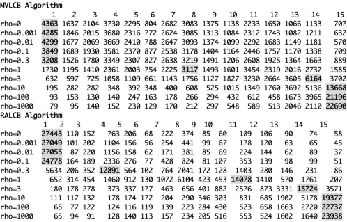
Figure 7: Record of total arms pulled in a single simulation by two algorithms under different $\rho$. The highlighted ones are the optimal arms under each $\rho$.

From Figure 7, we can conclude that:

1. Under all different $\rho$, the RALCB algorithm pulls the optimal arms more frequently than the MVLCB algorithm.

2. Both algorithms can distinguish the optimal arms from suboptimal arms better when $\rho$ is small.

We report the cumulative regrets in Figure 8,

\begin{overpic}[width=260.17464pt]{fig8.pdf} \put(400.0,200.0){MVLCB} \put(600.0,100.0){RALCB} \end{overpic}

Figure 8: Cumulative regret comparison averaged over 1000 runs for two algorithms over different choices of $\rho$.

From Figure 8, we observe the outperformance of RALCB over MVLCB when $\rho$ is small. But, the performance gap narrows as $\rho$ increases.

4.5 Exploration Term Analysis

To explain the performance difference, we compare the exploration terms of the lower confidence index for two algorithms under $t=10000$.

Algorithm	$T_{i,t}<77$	$T_{i,t}\geq 77$
MVLCB	$5\sqrt{x}+\rho\sqrt{x}$	$5\sqrt{x}+\rho\sqrt{x}$
RALCB	$33x\theta_{\textup{max}}^{2}+\rho\theta_{\textup{max}}\sqrt{x}$	$(16\sqrt{2x}+x)\theta_{\textup{max}}^{2}+\rho\theta_{\textup{max}}\sqrt{x}$

Table 1: Exploration term comparison under small and large $T_{i,t}$, where $x=2\log(2(t-1)^{2})/T_{j,t}$.

When $\rho$ is small, the influence from the second term of the exploration term is negligible (i.e., $\rho\sqrt{x}$ for MVLCB and $\rho\theta_{\textup{max}}\sqrt{x}$ for RALCB). From Table 1, we can conclude that:

1. In the exploration period (i.e., when $T_{i,t}$ is small), the RALCB algorithm will encourage exploration by assigning a large value to the exploration term.

2. In the exploitation period (i.e., when $T_{i,t}$ is large), all arms have been fully examined. Thus, the RALCB algorithm will focus on exploitation by assigning a low value to the exploration term.

3. The MVLCB fails to distinguish between exploration and exploitation periods but keeps using the same exploration function for both. As a result, suboptimal arms are still pulled during the late period of the simulation.

4. RALCB outperforms MVLCB by successfully distinguishing exploration and exploitation periods when $\rho$ is small.

When $\rho$ is large, the lower confidence indexes of two algorithms (i.e., $V^{\textup{MVLCB}}_{i,t}$ and $V^{\textup{RALCB}}_{i,t}$) converge to $(-\rho\hat{\mu}_{i,t}-\rho\sqrt{2\log(2t^{2})/T_{j,t}})$. As a consequence, the cumulative regret of RALCB coincides with MVLCB, as shown in Figure 8.

4.6 Summary Of Dependent Gaussian Bandits

Under the dependent scenario, we compare the performance of our algorithm with the MVLCB under different choices of correlation coefficients (i.e., we use $\lambda_{i,j}$ to denote the correlation coefficients between arm $i$ and arm $j$). As a starting point, we assume each pair of arms share the same correlation coefficients (i.e., $\lambda_{i,j}=\lambda$, $\forall i,j$). We are working on analyzing the performance changes as the correlations increase, where

$$\lambda=(0,0.2,0.5,1).$$

Figure 9 compares the performance of two algorithms under different correlations.

\begin{overpic}[width=208.13574pt]{fig9.1.pdf} \put(400.0,300.0){MVLCB} \put(300.0,150.0){RALCB} \end{overpic}

(a)

\begin{overpic}[width=208.13574pt]{fig9.2.pdf} \put(400.0,310.0){MVLCB} \put(300.0,150.0){RALCB} \end{overpic}

(b)

\begin{overpic}[width=208.13574pt]{fig9.3.pdf} \put(400.0,330.0){MVLCB} \put(300.0,150.0){RALCB} \end{overpic}

(c)

\begin{overpic}[width=208.13574pt]{fig9.4.pdf} \put(400.0,350.0){MVLCB} \put(300.0,150.0){RALCB} \end{overpic}

(d)

Figure 9: Cumulative regret analysis averaged over 1000 runs under a dependent scenario with $K=15$.

Based on Figure 9 , we can conclude that:

1. By varying $\lambda$, we can observe that the RALCB consistently outperforms the MVLCB when $\rho$ is small, but the expected regret gap for the two algorithms narrows as $\rho$ increases.

2. With increasing $\lambda$, two algorithms’ performance converges.

3. The performance of both algorithms is insensitive to changes in correlations among arms.

Figure 10 illustrates the influence of correlation on the performance of the RALCB algorithm under different risk aversion $\rho$ parameters.

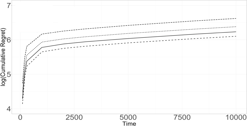
(a) Cumulative regret for $\rho=10^{-3}$

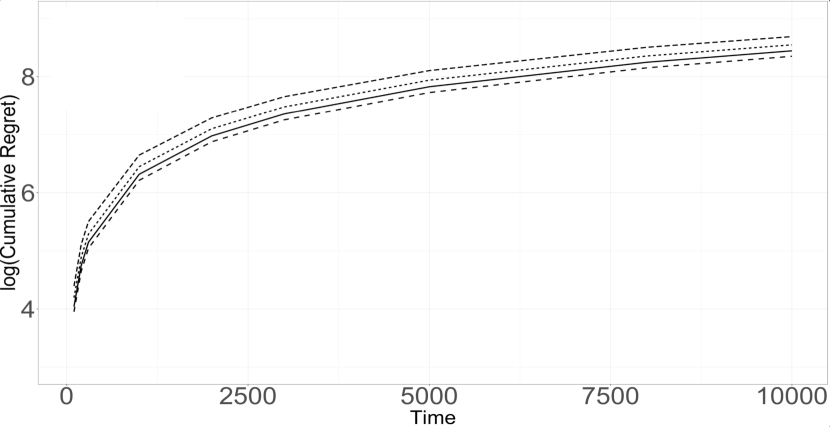
(b) Cumulative regret for $\rho=1$

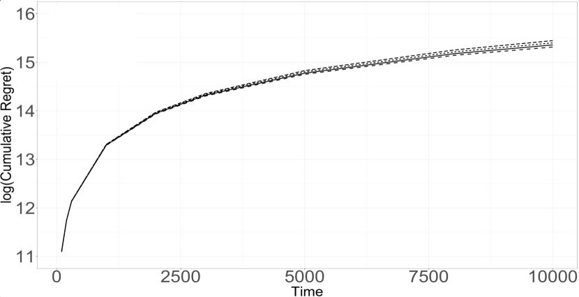
(c) Cumulative regret for $\rho=10^{3}$

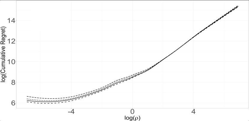
(d) Cumulative regret comparison over different $\rho$

Figure 10: Cumulative regret comparison over different choices of $\rho$. In the above plots, the short dashed line represents the cumulative regret of the case when correlation $\lambda=1$. The dotted line represents the cumulative regret of the case when correlation $\lambda=0.5$. The solid line represents the cumulative regret of the case when correlation $\lambda=0.2$ and the dashed line represents the cumulative regret of the independent case.

Based on Figure 10, we can conclude that:

1. For the RALCB algorithm, a higher correlation among arms will lead to a higher expected regret.

2. As $\rho$ grows, the impact of correlation on expected regret decreases.

4.7 Financial Data

In this section, we design experiments and evaluate the performance of our proposed algorithm (i.e., the RALCB algorithm) in portfolio selection to the performance of UCB algorithm, the $\epsilon$-greedy algorithm and equally weighted (EW) strategy. In the experiment, we implement actual stock market data to test the performance of the above four algorithms. The dataset we use is S&P500, which is the most frequent trading stock market data. We select 30 stocks from the S&P500 stock pool based on size, age, and earning per share: AAPL, MSFT, UNH, JNJ, XOM, PNR, AIG, VNO, DISH, NWL, BK, STT, CL, HIG, ED, CMA, ALL, AMAT, BSX, MU, HAL, RCL, CCL, APA, HRL, AEE, FAST, TRMB, NWL, AFL. In our dataset, we have weekly observations of all 30 ETFs over the time period $1996/02/26$ to $2021/02/26$.

Figure 11 presents the change in portfolio wealth by following different algorithms over time. We notice that when the market turns down during the middle of the timeline, wealth for MAB-based algorithms drops dramatically. The main reason is that MAB-based algorithms must spend time learning new parameters because the underlying parameters estimated from the history are no longer valid. Overall, the RALCB algorithm achieves the best long-term performance and the highest wealth at the end.

\begin{overpic}[width=303.53267pt]{fig11.pdf} \put(800.0,400.0){RALCB} \put(900.0,300.0){EW} \put(850.0,250.0){SP500} \put(850.0,200.0){$\epsilon$-greedy} \put(900.0,100.0){UCB} \end{overpic}

Figure 11: The curves of cumulative wealth across the investment periods (1996-2021) for different algorithms.

To compare the performance of four investment algorithms, we use the standard criteria in finance proposed by Zhu et al. (2019): Cumulative Wealth (CW), Volatility (VO), Sharpe Ratio (SR) and Maximum Drawdown (MDD).

Table 2 summarizes portfolio performance as measured by the SR, CW, and VO for all benchmarks tested, with the bold values indicating the winners. The risk-free (Rf) rate, which is based on the historical average of the 10-Year Treasury Rate, is assumed to be 4.38% yearly for generating the SR. Among all algorithms, RALCB algorithm is the one with the highest cumulative wealth. However, EW does a better job of risk-return balancing than RALCB. The main reason is that the RALCB algorithm only permits the investment of one stock per period, which naturally increases the portfolio’s volatility.

1996-2021	UCB	RALCB	EGREEDY	EW
CW	2.3579	7.4988	2.4741	7.3485
VO	0.3777	0.2926	0.3151	0.1921
SR (Rf=4.38%)	-0.0784	0.1480	-0.0490	0.7330
MDD	0.9191	0.7432	0.3648	0.2978

Table 2: Performance of four different algorithms on real data. RALCB outperforms the other algorithms in terms of wealth accumulation. EW does a better job of risk-return balancing than RALCB.

In our next application, the arms consist of the following S&P 500 sector ETFs: GDX, IBB, ITB, IYE, IYR, KBE, KRE, OIH, SMH, VNQ, XHB, XLB, XLF, XLI, XLK, XLP, XLU, XLV, XLY, XME, XOP, XRT. In our dataset, we have daily observations of all 22 ETFs over the time period $2006/06/22$ to $2022/11/18$.

Figure 12 presents the change in portfolio wealth by following different algorithms over time. We notice that, by investing in ETFs, the RALCB algorithm achieves better long-term performance than the other algorithms.

\begin{overpic}[width=303.53267pt]{fig12.pdf} \put(750.0,400.0){RALCB} \put(850.0,300.0){EW} \put(850.0,200.0){UCB} \put(850.0,100.0){$\epsilon$-greedy} \end{overpic}

Figure 12: The curves of cumulative wealth across the investment periods (2006-2022) for different algorithms.

Again, we use the standard criteria in finance proposed by Zhu et al. (2019) to compare the performance of four investment algorithms:

2006-2022	UCB	RALCB	EGREEDY	EW
CW	2.5629	4.8620	2.1932	3.7621
VO	0.1004	0.0824	0.1444	0.1056
SR (Rf=4.38%)	-0.2771	-0.1396	-0.2205	-0.2190
MDD	0.6579	0.4213	0.6588	0.5616

Table 3: Performance of four different algorithms on ETFs investment. RALCB outperforms the other algorithms in terms of all financial criteria.

Table 3 summarizes portfolio performance as measured by the SR, CW, and VO for all benchmarks tested, with the bold values indicating the winners. The risk-free (Rf) rate is again assumed to be 4.38% yearly.

5 Proofs

This section consists of two parts. First, we derive the high-probability confidence bounds on the empirical mean-variance through an application of the Chernoff–Hoeffding inequality. In the second part, we report a complete analysis of the learning regret of the RALCB algorithm. Unless otherwise stated, all identities and inequalities between random variables are stated in $\mathbb{P}$-a.s. in the following proofs.

5.1 Concentration Analysis

To derive a high-probability bound on the expected pseudo regret, we need to build high-probability confidence bounds on empirical mean and variance through an application of the Chernoff–Hoeffding inequality. Recall that we assume that the rewards of each arm belong to the class of sub-Gaussian random variables. Therefore, we analyze the concentration of empirical mean and variance via sub-Gaussian and sub-exponential distributions. In this section, we let $\left\{X_{t}\right\}_{t\geq 0}$ be i.i.d. sub-Gaussian random variables with parameter $\theta^{2}$, mean $\mu$, and variance $\sigma^{2}$. We start by providing a concentration bound for the empirical mean $\hat{\mu}_{n}\mathrel{\mathop{\mathchar 58\relax}}=\frac{1}{n}\sum_{t=1}^{n}X_{t}$.

Lemma 5.1.

For every $n>0$ and $\delta\in(0,1)$, with probability at least $1-\delta$,

$$|\hat{\mu}_{n}-\mu|\leq\theta\sqrt{\frac{2\log(2/\delta)}{n}}.$$ (12)

Proof.

According to Markov’s inequality, for all $a\geq 0$,

$$\mathbb{P}[|\hat{\mu}_{n}-\mu|\geq a]\leq\mathbb{P}\Big{[}\sum_{t=1}^{n}(X_{t}-\mu)\leq-na\Big{]}+\mathbb{P}\Big{[}\sum_{t=1}^{n}(X_{t}-\mu)\geq na\Big{]}\leq 2e^{-na^{2}/(2\theta^{2})}.$$

The result thus follows by taking $\delta=2e^{-na^{2}/(2\theta^{2})}$. ∎

Now we derive a concentration inequality for the sample variance $\hat{\sigma}_{n}^{2}\mathrel{\mathop{\mathchar 58\relax}}=\frac{1}{n}\sum_{t=1}^{n}(X_{t}-\hat{\mu}_{n})^{2}$. Its proof uses the notion of sub-exponential random variables. Recall that a random variable $Z$ is called sub-exponential with parameter $\lambda>0$ if $\mathbb{E}[Z]=0$ and $\mathbb{E}[e^{sZ}]\leq e^{s^{2}\lambda^{2}/2}$ for all $s\in\mathbb{R}$ with $|s|\leq 1/\lambda$; see, e.g., Wainwright (2019) and Rigollet and Hütter (2015).

Lemma 5.2.

For every $n>0$ and $\delta\in(0,1)$, we have that with probability at least $1-\delta$,

$$\left|\hat{\sigma}_{n}^{2}-\sigma^{2}+(\hat{\mu}_{n}-\mu)^{2}\right|\leq 32\theta^{2}\max\left(\sqrt{\frac{\log(2/\delta)}{n}},\frac{2\log(2/\delta)}{n}\right).$$ (13)

Proof.

We may assume without loss of generality that $\mu=0$. Lemma 1.12 in Rigollet and Hütter (2015) states that $Z_{t}\mathrel{\mathop{\mathchar 58\relax}}=X_{t}^{2}$ is sub-exponential with parameter $16\theta^{2}$. An application of Proposition 2.9 in Wainwright (2019) hence yields that

$$\mathbb{P}\left(\left|\frac{1}{n}\sum_{i=1}^{n}(X_{i})^{2}-\sigma^{2}\right|>a\right)\leq 2\exp\left(-\frac{n}{2}g(a)\right),$$ (14)

where $g(a)\mathrel{\mathop{\mathchar 58\relax}}=\min(\frac{a^{2}}{512\theta^{4}},\frac{a}{32\theta^{2}})$. Moreover,

$$\left|\frac{1}{n}\sum_{i=1}^{n}(X_{i})^{2}-\sigma^{2}\right|=\left|\hat{\sigma}_{n}^{2}-\sigma^{2}+\hat{\mu}_{n}^{2}\right|.$$

Therefore, we have,

$$\mathbb{P}\left(\left|\hat{\sigma}_{n}^{2}-\sigma^{2}+\hat{\mu}_{n}^{2}\right|>a\right)\leq 2\exp\left(-\frac{n}{2}g(a)\right).$$ (15)

By setting $\delta\mathrel{\mathop{\mathchar 58\relax}}=2\exp\left(-\frac{n}{2}g(a)\right)$ and writing $a$ in terms of $\delta$ on the left side of the inequality (15), we obtain:

$$\mathbb{P}\left(\left|\hat{\sigma}_{n}^{2}-\sigma^{2}+\hat{\mu}_{n}^{2}\right|>32\theta^{2}\max\left(\sqrt{\frac{\log(2/\delta)}{n}},\frac{2\log(2/\delta)}{n}\right)\right)\leq\delta.$$ (16)

Alternatively, with a probability of at least $1-\delta$,

$$\left|\hat{\sigma}_{n}^{2}-\sigma^{2}+(\hat{\mu}_{n}-\mu)^{2}\right|\leq 32\theta^{2}\max\left(\sqrt{\frac{\log(2/\delta)}{n}},\frac{2\log(2/\delta)}{n}\right).$$

∎

In our analysis, we assume the rewards of each arm belong to the class of sub-Gaussian random variables with different parameters. With Lemma 5.1 and Lemma 5.2, we can construct the following high-probability confidence bounds on the empirical mean-variance.

Lemma 5.3.

Suppose that for each arm $i$, $X^{i}_{1},...,X^{i}_{t}$ are i.i.d. sub-Gaussian random variables with parameter $\theta_{i}^{2}$, mean $\mu_{i}$, and variance $\sigma_{i}^{2}$, as well as empirical mean $\tilde{\mu}_{i,t}$ and variance $\tilde{\sigma}_{i,t}^{2}$. Let furthermore

$$\theta_{\max}^{2}\mathrel{\mathop{\mathchar 58\relax}}=\max_{i=1,\ldots,K}\theta_{i}^{2},$$

$\widehat{\mathrm{MV}}^{\rho}_{i,t}\mathrel{\mathop{\mathchar 58\relax}}=\tilde{\sigma}_{i,t}^{2}-\rho\tilde{\mu}_{i,t}$, $\mathrm{MV}^{\rho}_{i}\mathrel{\mathop{\mathchar 58\relax}}=\sigma_{i}^{2}-\rho\mu_{i}$ and

$$\varphi(x)\mathrel{\mathop{\mathchar 58\relax}}=32\theta_{\max}^{2}\max\left(\sqrt{x/2},x\right)+\theta_{\max}^{2}x+\rho\theta_{\max}\sqrt{x}.$$

Then

$$\mathbb{P}\left[\min_{\begin{subarray}{c}i=1,\ldots,K\\ t=1,\ldots,n\end{subarray}}\left|\widehat{\mathrm{MV}}^{\rho}_{i,t}-\mathrm{MV}^{\rho}_{i}\right|\geq\varphi\left(\frac{2\log(2/\delta)}{n}\right)\right]\leq 2nK\delta.$$

Proof.

Let

$$A_{i,t}\mathrel{\mathop{\mathchar 58\relax}}=\left\{|\tilde{\mu}_{i,t}-\mu_{i}|\leq\theta_{\max}\sqrt{\frac{2\log(2/\delta)}{t}}\right\},$$

and

$$B_{i,t}\mathrel{\mathop{\mathchar 58\relax}}=\left\{\left|\tilde{\sigma}_{i,t}^{2}-\sigma_{i}^{2}+(\tilde{\mu}_{i,t}-\mu_{i})^{2}\right|\leq 32\theta_{\max}^{2}\max\left(\sqrt{\frac{\log(2/\delta)}{t}},\frac{2\log(2/\delta)}{t}\right)\right\}.$$

By Lemma 5.1 and 5.2, we have $\mathbb{P}(A_{i,t})\geq 1-\delta$ and $\mathbb{P}(B_{i,t})\geq 1-\delta$. Now, we define

$$C_{i,t}\mathrel{\mathop{\mathchar 58\relax}}=\left\{\left|\widehat{\mathrm{MV}}^{\rho}_{i,t}-\mathrm{MV}^{\rho}_{i}\right|\leq\varphi\left(\frac{2\log(2/\delta)}{t}\right)\right\}.$$

According to the triangle inequality, we have for any $i$ and $t$:

$$\left|\widehat{\mathrm{MV}}^{\rho}_{i,t}-\mathrm{MV}^{\rho}_{i}\right| \leq\left|\hat{\sigma}_{i,t}^{2}-\sigma_{i}^{2}\right|+\rho|\hat{\mu}_{i,t}-\mu_{i}|$$

$$\leq\left|\hat{\sigma}_{i,t}^{2}-\sigma_{i}^{2}+(\hat{\mu}_{i,t}-\mu_{i})^{2}\right|+(\hat{\mu}_{i,t}-\mu_{i})^{2}+\rho|\hat{\mu}_{i,t}-\mu_{i}|.$$

As a result, for any $i$ and $t$, $A_{i,t}\cap B_{i,t}\subseteq C_{i,t}$. Through the union bound, we have:

$$\mathbb{P}\left[\bigcup_{i=1}^{K}\bigcup_{t=1}^{n}C_{i,t}^{c}\right]\leq\sum_{i,t}\mathbb{P}\left[C_{i,t}^{c}\right]\leq\sum_{i,t}\mathbb{P}\left[A_{i,t}^{c}\cup B_{i,t}^{c}\right]\leq\sum_{i,t}(\mathbb{P}\left[A_{i,t}^{c}\right]+\mathbb{P}\left[B_{i,t}^{c}\right])\leq 2nK\delta.$$

∎

.

5.2 Regret Analysis

Given the definition of regret in Equation (3), Sani et al. (2012) derived the following upper bound of the regret. For $i^{\rho}_{0}\in\mathop{\rm arg\,min}_{i\in\mathcal{A}}\textup{MV}^{\rho}_{i}$, $\widehat{\Delta}_{i}\mathrel{\mathop{\mathchar 58\relax}}=\left(\hat{\sigma}_{i,n}^{2}-\sigma_{i^{\rho}_{0}}^{2}\right)-\rho\left(\hat{\mu}_{i,n}-\mu_{i^{\rho}_{0}}\right)$, and $\widehat{\Gamma}_{i,h}^{2}\mathrel{\mathop{\mathchar 58\relax}}=\left(\hat{\mu}_{i,n}-\hat{\mu}_{h,n}\right)^{2}$, the regret for a learning algorithm $\pi_{t}$ over $n$ rounds is upper bounded by

$$\mathcal{R}(\pi)\leq\frac{1}{n}\sum_{i=1}^{K}T_{i,n}\widehat{\Delta}_{i}+\frac{1}{n^{2}}\sum_{i=1}^{K}\sum_{h\neq i}T_{i,n}T_{h,n}\widehat{\Gamma}_{i,h}^{2}.$$ (17)

The upper bound suggests that a bound on the pulls is sufficient to bound the regret. Next, we introduce the pseudo regret for a learning algorithm $\pi_{t}$ over $n$ rounds, which can be defined as:

$$\widetilde{\mathcal{R}}(\pi)\mathrel{\mathop{\mathchar 58\relax}}=\frac{1}{n}\sum_{i=1}^{K}T_{i,n}\Delta_{i}+\frac{3}{n^{2}}\sum_{i=1}^{K}\sum_{h\neq i}T_{i,n}T_{h,n}\Gamma_{i,h}^{2},$$ (18)

where $\Delta_{i}\mathrel{\mathop{\mathchar 58\relax}}=\left(\sigma_{i}^{2}-\sigma_{i^{\rho}_{0}}^{2}\right)-\rho\left(\mu_{i}-\mu_{i^{\rho}_{0}}\right)$ and $\Gamma_{i,h}^{2}\mathrel{\mathop{\mathchar 58\relax}}=\left(\mu_{i}-\mu_{h}\right)^{2}$. As in Zhu and Tan (2020), one proves that also in our more general setting, the following inequality remains true,

$$\mathbb{E}[\mathcal{R}(\pi)]\leq\mathbb{E}[\widetilde{\mathcal{R}}(\pi)]+\frac{5}{n}\sum_{i=1}^{K}\sigma_{i}^{2}.$$ (19)

The same holds for the following inequality from Zhu and Tan (2020),

$$\mathbb{E}[\widetilde{\mathcal{R}}(\pi)]\leq\frac{1}{n}\sum_{i\neq i^{\rho}_{0}}\mathbb{E}[T_{i,n}](\Delta_{i}+2\Gamma_{i,\max}^{2}),$$ (20)

where $\Gamma_{i,\max}^{2}\mathrel{\mathop{\mathchar 58\relax}}=\max\left\{\left(\mu_{i}-\mu_{h}\right)^{2}\mathrel{\mathop{\mathchar 58\relax}}h=1,\ldots,K\right\}.$ Equation (20) shows that to recover a bound on the expected pseudo regret, it suffices to bound the number of pulls of each suboptimal arm. Following an idea of Sani et al. (2012), we now derive an upper bound for the number of pulls in expectation.

Lemma 5.4.

Suppose that $i^{\rho}_{0}\in\mathop{\rm arg\,min}_{i\in\mathcal{A}}\textup{MV}^{\rho}_{i}$. The expected number of pulls of any suboptimal arm $i\neq i^{\rho}_{0}$ in RALCB can be upper bounded by

$$\mathbb{E}\left[T_{i,n}\right]\leq\frac{2\log(2/\delta)}{\varphi^{-1}(\Delta_{i}/2)}+1+2n^{2}K\delta,$$ (21)

where $\varphi^{-1}$ is the inverse function of $\varphi$ and is given by

$$\varphi^{-1}(x)=\left\{\begin{array}[]{ll}\left(\frac{-(\rho\theta_{\textup{max}}+16\sqrt{2}\theta_{\textup{max}}^{2})+\sqrt{(\rho\theta_{\textup{max}}+16\sqrt{2}\theta_{\textup{max}}^{2})^{2}+4\theta_{\textup{max}}^{2}x}}{2\theta_{\textup{max}}^{2}}\right)^{2}&\quad x\in[0,\frac{17}{2}\theta_{\textup{max}}^{2}+\frac{\sqrt{2}}{2}\rho\theta_{\textup{max}}),\\ \left(\frac{-\rho\theta_{\textup{max}}+\sqrt{\rho^{2}\theta_{\textup{max}}^{2}+132\theta_{\textup{max}}^{2}x}}{66\theta_{\textup{max}}^{2}}\right)^{2}&\quad x\in[\frac{17}{2}\theta_{\textup{max}}^{2}+\frac{\sqrt{2}}{2}\rho\theta_{\textup{max}},\infty).\end{array}\right.$$

Proof.

We first construct the following events:

$$A_{i,t}\mathrel{\mathop{\mathchar 58\relax}}=\left\{|\hat{\mu}_{i,t}-\mu_{i}|\leq\theta_{\max}\sqrt{\frac{2\log(2/\delta)}{t}}\right\},$$

and

$$B_{i,t}\mathrel{\mathop{\mathchar 58\relax}}=\left\{\left|\hat{\sigma}_{i,t}^{2}-\sigma_{i}^{2}+(\hat{\mu}_{i,t}-\mu_{i})^{2}\right|\leq 16\theta_{\max}^{2}\max\left(\sqrt{\frac{\log(2/\delta)}{t}},\frac{2\log(2/\delta)}{t}\right)\right\}.$$

By Lemma 5.1 and 5.2, we have $\mathbb{P}(A_{i,t})\geq 1-\delta$ and $\mathbb{P}(B_{i,t})\geq 1-\delta$.

Now, we can define a high–probability event $\mathcal{E}_{\delta}$ as:

$$\mathcal{E}_{\delta}\mathrel{\mathop{\mathchar 58\relax}}=\bigcap_{i=1}^{K}\bigcap_{t=1}^{n}\left(A_{i,t}\cap B_{i,t}\right),$$

Through the union bound, we have:

$$\mathbb{P}\left[\mathcal{E}_{\delta}^{c}\right]=\mathbb{P}\left[\bigcup_{i=1}^{K}\bigcup_{t=1}^{n}\left(A_{i,t}\cap B_{i,t}\right)^{c}\right]\leq\sum_{i,t}\mathbb{P}\left[A_{i,t}^{c}\cup B_{i,t}^{c}\right]\leq\sum_{i,t}(\mathbb{P}\left[A_{i,t}^{c}\right]+\mathbb{P}\left[B_{i,t}^{c}\right])\leq 2nK\delta.$$

Now let us consider the moment when arm $i$ is selected at some time step $t$, where $i\neq i^{\rho}_{0}$. It means that its lower confidence index was lower than that of the optimal arm $i^{\rho}_{0}$ (i.e., $V_{i,t-1}\leq V_{i^{\rho}_{0},t-1}$):

$$\hat{\sigma}_{i,t-1}^{2}-\rho\hat{\mu}_{i,t-1}-\varphi\left(\frac{2\log(2/\delta)}{T_{i,t-1}}\right)\leq\hat{\sigma}_{i^{\rho}_{0},t-1}^{2}-\rho\hat{\mu}_{i^{\rho}_{0},t-1}-\varphi\left(\frac{2\log(2/\delta)}{T_{i^{\rho}_{0},t-1}}\right).$$

We also know that on the event $\mathcal{E}_{\delta}$:

$$\sigma^{2}_{i}-\rho\mu_{i}-\varphi\left(\frac{2\log(2/\delta)}{T_{i,t-1}}\right)\leq\hat{\sigma}_{i,t-1}^{2}-\rho\hat{\mu}_{i,t-1},$$

and

$$\hat{\sigma}_{i^{\rho}_{0},t-1}^{2}-\rho\hat{\mu}_{i^{\rho}_{0},t-1}-\varphi\left(\frac{2\log(2/\delta)}{T_{i^{\rho}_{0},t-1}}\right)\leq\sigma^{2}_{i^{\rho}_{0}}-\rho\mu_{i^{\rho}_{0}}.$$

Combining the last three inequalities, we have

$$\sigma^{2}_{i}-\rho\mu_{i}-2\varphi\left(\frac{2\log(2/\delta)}{T_{i,t-1}}\right)\leq\sigma^{2}_{i^{\rho}_{0}}-\rho\mu_{i^{\rho}_{0}}\quad\textup{on}\;\;\mathcal{E}_{\delta}.$$

Accordingly, we have:

$$\Delta_{i}\leq 2\varphi\left(\frac{2\log(2/\delta)}{T_{i,t-1}}\right)\quad\textup{on}\;\;\mathcal{E}_{\delta}.$$ (22)

Before solving for $T_{i,t-1}$, we first analyze the function $\varphi(x)$ for $x\geq 0$:

$$\varphi(x)\mathrel{\mathop{\mathchar 58\relax}}=32\theta_{\textup{max}}^{2}\max\left(\sqrt{x/2},x\right)+\theta_{\textup{max}}^{2}x+\rho\theta_{\textup{max}}\sqrt{x}.$$

Equivalently, we have:

$$\varphi(x)=\left\{\begin{array}[]{ll}32\theta_{\textup{max}}^{2}\sqrt{x/2}+\rho\theta_{\textup{max}}\sqrt{x}+\theta_{\textup{max}}^{2}x&\quad x\in[0,\frac{1}{2}),\\ 33\theta_{\textup{max}}^{2}x+\rho\theta_{\textup{max}}\sqrt{x}&\quad x\in[\frac{1}{2},\infty).\end{array}\right.$$

Based on the above representation, we can easily show that $\varphi(x)$ is continuous and strictly increasing on $x\in[0,\infty)$. Therefore, we can derive the inverse $\varphi^{-1}(\cdot)$ for $\varphi(\cdot)$:

$$\varphi^{-1}(x)=\left\{\begin{array}[]{ll}\left(\frac{-(\rho\theta_{\textup{max}}+16\sqrt{2}\theta_{\textup{max}}^{2})+\sqrt{(\rho\theta_{\textup{max}}+16\sqrt{2}\theta_{\textup{max}}^{2})^{2}+4\theta_{\textup{max}}^{2}x}}{2\theta_{\textup{max}}^{2}}\right)^{2}&\quad x\in[0,\frac{17}{2}\theta_{\textup{max}}^{2}+\frac{\sqrt{2}}{2}\rho\theta_{\textup{max}}),\\ \left(\frac{-\rho\theta_{\textup{max}}+\sqrt{\rho^{2}\theta_{\textup{max}}^{2}+132\theta_{\textup{max}}^{2}x}}{66\theta_{\textup{max}}^{2}}\right)^{2}&\quad x\in[\frac{17}{2}\theta_{\textup{max}}^{2}+\frac{\sqrt{2}}{2}\rho\theta_{\textup{max}},\infty).\end{array}\right.$$

By applying the inverse function into inequality (22), we obtain:

$$T_{i,t-1}\leq\frac{2\log(2/\delta)}{\varphi^{-1}(\Delta_{i}/2)}\quad\textup{on}\;\;\mathcal{E}_{\delta}.$$ (23)

Let time $t$ be the last time when arm $i$ is pulled until the final round $n$, then $T_{i,t-1}=T_{i,n}-1$ and

$$T_{i,n}\leq\frac{2\log(2/\delta)}{\varphi^{-1}(\Delta_{i}/2)}+1\quad\textup{on}\;\;\mathcal{E}_{\delta}.$$

We now move from the previous high–probability bound to a bound in expectation. Clearly,

$$\mathbb{E}\left[T_{i,n}\right]=\mathbb{E}\left[T_{i,n}\mathbb{I}_{\mathcal{E}_{\delta}}\right]+\mathbb{E}\left[T_{i,n}\mathbb{I}_{\mathcal{E}_{\delta}^{c}}\right]\leq\mathbb{E}\left[T_{i,n}\mathbb{I}_{\mathcal{E}_{\delta}}\right]+n\mathbb{P}\left[\mathcal{E}_{\delta}^{c}\right].$$

By $\mathbb{P}\left[\mathcal{E}_{\delta}^{c}\right]\leq 2nK\delta$, we have

$$\mathbb{E}\left[T_{i,n}\right]\leq\frac{2\log(2/\delta)}{\varphi^{-1}(\Delta_{i}/2)}+1+2n^{2}K\delta.$$ (24)

∎

We can now proceed with the proof of Theorem 3.1.

Proof of Theorem 3.1.

We start with deriving an upper bound for the expected regret. By substituting the result of Lemma 5.4 into (20) and tuning the confidence level parameter $\delta\mathrel{\mathop{\mathchar 58\relax}}=1/n^{2}$, we receive the following upper bound for the expected pseudo-regret,

$$\mathbb{E}[\widetilde{\mathcal{R}}(\pi)]\leq\frac{1}{n}\sum_{i\neq i^{\rho}_{0}}\left(\frac{4\log(\sqrt{2}n)}{\varphi^{-1}(\Delta_{i}/2)}+1+2K\right)(\Delta_{i}+2\Gamma_{i,\max}^{2}).$$

By (19), the expected regret of the RALCB algorithm for $n$ rounds can be upper bounded as follows,

$$\mathbb{E}[\mathcal{R}(\pi)]\leq\frac{1}{n}\sum_{i\neq i^{\rho}_{0}}\left(\frac{4\log(\sqrt{2}n)}{\varphi^{-1}(\Delta_{i}/2)}+1+2K\right)(\Delta_{i}+2\Gamma_{i,\max}^{2})+\frac{5}{n}\sum_{i=1}^{K}\sigma_{i}^{2}.$$

∎

Now, we can turn to the proof of Theorem 3.2.

Proof of Theorem 3.2.

First, we derive the claimed upper bound for the regret. By the definitions in Section 5.2, we have:

$$\widehat{\Delta}_{i}=\Delta_{i}+\left(\hat{\sigma}_{i,T{i,n}}^{2}-\sigma_{i}^{2}\right)-\rho\left(\hat{\mu}_{i,T{i,n}}-\mu_{i}\right),$$

and

$$\left|\widehat{\Gamma}_{i,h}\right|=\left|\Gamma_{i,h}-\mu_{i}+\mu_{h}+\hat{\mu}_{i,T{i,n}}-\hat{\mu}_{h,T{h,n}}\right|.$$

By Lemma 5.3, with a high probability $1-2nK\delta$, we have

$$\widehat{\Delta}_{i}\leq\Delta_{i}+\varphi\left(\frac{2\log(2/\delta)}{T_{i,n}}\right),$$

and

$$\left|\widehat{\Gamma}_{i,h}\right|\leq\left|\Gamma_{i,h}\right|+\theta\sqrt{\frac{2\log(2/\delta)}{T{i,n}}}+\theta\sqrt{\frac{2\log(2/\delta)}{T_{h,n}}}.$$

According to (17),

$$\mathcal{R}(\pi)$$

$$\leq\frac{1}{n}\sum_{i=1}^{K}T_{i,n}\widehat{\Delta}_{i}+\frac{1}{n^{2}}\sum_{i=1}^{K}\sum_{h\neq i}T_{i,n}T_{h,n}\widehat{\Gamma}_{i,h}^{2}$$

$$\leq\frac{1}{n}\sum_{i=1}^{K}T_{i,n}\left(\Delta_{i}+\varphi\left(\frac{2\log(2/\delta)}{T_{i,n}}\right)\right)$$

$$+\frac{1}{n^{2}}\sum_{i=1}^{K}\sum_{h\neq i}T_{i,n}T_{h,n}\left(\left|\Gamma_{i,h}\right|+\theta\sqrt{\frac{2\log(2/\delta)}{T{i,n}}}+\theta\sqrt{\frac{2\log(2/\delta)}{T_{h,n}}}\right)^{2}$$

$$\leq\frac{1}{n}\sum_{i=1}^{K}T_{i,n}\Delta_{i}+\frac{1}{n}\sum_{i=1}^{K}T_{i,n}\varphi\left(\frac{2\log(2/\delta)}{T_{i,n}}\right)+\frac{2}{n^{2}}\sum_{i=1}^{K}\sum_{h\neq i}T_{i,n}T_{h,n}\Gamma_{i,h}^{2}$$

$$+\frac{2\theta^{2}\sqrt{2}}{n^{2}}\sum_{i=1}^{K}\sum_{h\neq i}T_{h,n}\log(2/\delta)+\frac{2\theta^{2}\sqrt{2}}{n^{2}}\sum_{i=1}^{K}\sum_{i\neq i}T_{h,n}\log(2/\delta)$$

$$\leq\frac{1}{n}\sum_{i=1}^{K}T_{i,n}\Delta_{i}+\frac{2}{n^{2}}\sum_{i=1}^{K}\sum_{h\neq i}T_{i,n}T_{h,n}\Gamma_{i,h}^{2}$$

$$+32\theta_{\textup{max}}\max\left(\sqrt{\frac{2K\log 2/\delta}{n}},\frac{K\log 2/\delta}{n}\right)+(1+4\sqrt{2})\frac{K\theta_{\textup{max}}\log 2/\delta}{n}+\rho\theta_{\textup{max}}\sqrt{\frac{2K\log 2/\delta}{n}},$$

where in the next to last passage we used Jensen’s inequality for concave functions and rough upper on other terms $(K-1<K,\sum_{i}T_{i,n}\leq n)$. By recalling the definition of $\widetilde{\mathcal{R}}(\pi)$ we finally obtain

$$\mathcal{R}(\pi)$$

$$\leq\widetilde{\mathcal{R}}(\pi)+32\theta_{\textup{max}}\max\left(\sqrt{\frac{K\log 2/\delta}{n}},\frac{2K\log 2/\delta}{n}\right)+(1+2\sqrt{2})\frac{2K\theta_{\textup{max}}\log 2/\delta}{n}$$

$$+\rho\theta_{\textup{max}}\sqrt{\frac{2K\log 2/\delta}{n}}$$

$$\leq\widetilde{\mathcal{R}}(\pi)+\frac{\varphi\left(\frac{2K\log 2/\delta}{n}\right)}{\theta_{\textup{max}}}+\frac{4\sqrt{2}K\theta_{\textup{max}}\log 2/\delta}{n},$$

with probability $1-2nK\delta$. Based on (20) and Lemma 5.4, we can find an upper bound for $\widetilde{\mathcal{R}}(\pi)$:

$$\widetilde{\mathcal{R}}(\pi) \leq\frac{1}{n}\sum_{i\neq i^{\rho}_{0}}T_{i,n}(\Delta_{i}+2\Gamma_{i,\max}^{2})$$

$$\leq\frac{1}{n}\sum_{i\neq i^{\rho}_{0}}\left(\frac{2\log(2/\delta)}{\varphi^{-1}(\Delta_{i}/2)}+1\right)(\Delta_{i}+2\Gamma_{i,\max}^{2}).$$

Combining the above results gives us the stated regret bound.∎

References

- Agrawal (1995) Agrawal, R. (1995). Sample mean based index policies by regret for the multi-armed bandit problem. Advances in Applied Probability, 27(4):1054–1078.
- Agrawal and Goyal (2012) Agrawal, S. and Goyal, N. (2012). Analysis of Thompson sampling for the multi-armed bandit problem. In Proceedings of the 25th Annual Conference on Learning Theory, volume 23 of Proceedings of Machine Learning Research, pages 39.1–39.26, Edinburgh, Scotland. PMLR.
- Auer et al. (2002) Auer, P., Cesa-Bianchi, N., and Fischer, P. (2002). Finite-time analysis of the multiarmed bandit problem. Machine Learning, 47(2):235–256.
- Boldrini et al. (2018) Boldrini, S., De Nardis, L., Caso, G., Le, M. T. P., Fiorina, J., and Di Benedetto, M.-G. (2018). muMAB: A multi-armed bandit model for wireless network selection. Algorithms, 11(2).
- Chapelle and Li (2011) Chapelle, O. and Li, L. (2011). An empirical evaluation of Thompson sampling. In Advances in Neural Information Processing Systems, volume 24. Curran Associates, Inc.
- Durand et al. (2018) Durand, A., Achilleos, C., Iacovides, D., Strati, K., Mitsis, G. D., and Pineau, J. (2018). Contextual bandits for adapting treatment in a mouse model of de novo carcinogenesis. In Proceedings of the 3rd Machine Learning for Healthcare Conference, volume 85 of Proceedings of Machine Learning Research, pages 67–82. PMLR.
- Galichet et al. (2014) Galichet, N., Sebag, M., and Teytaud, O. (2014). Exploration vs exploitation vs safety: Risk-averse multi-armed bandits. CoRR, abs/1401.1123.
- Gupta et al. (2021) Gupta, S., Chaudhari, S., Joshi, G., and Yagan, O. (2021). Multi-armed bandits with correlated arms. IEEE Transactions on Information Theory, 67(10):6711–6732.
- Hoeffding (1963) Hoeffding, W. (1963). Probability inequalities for sums of bounded random variables. Journal of the American Statistical Association, 58(301):13–30.
- Kagrecha et al. (2019) Kagrecha, A., Nair, J., and Jagannathan, K. P. (2019). Distribution oblivious, risk-aware algorithms for multi-armed bandits with unbounded rewards. CoRR, abs/1906.00569.
- Lai and Robbins (1985) Lai, T. and Robbins, H. (1985). Asymptotically efficient adaptive allocation rules. Advances in Applied Mathematics, 6(1):4–22.
- Liu et al. (2021) Liu, X., Derakhshani, M., Lambotharan, S., and van der Schaar, M. (2021). Risk-aware multi-armed bandits with refined upper confidence bounds. IEEE Signal Processing Letters, 28:269–273.
- Markowitz (1968) Markowitz, H. M. (1968). Portfolio Selection: Efficient Diversification of Investments. Yale University Press.
- Mary et al. (2015) Mary, J., Gaudel, R., and Preux, P. (2015). Bandits and recommender systems. In Machine Learning, Optimization, and Big Data, pages 325–336, Cham. Springer International Publishing.
- May et al. (2012) May, B. C., Korda, N., Lee, A., and Leslie, D. S. (2012). Optimistic Bayesian sampling in contextual-bandit problems. Journal of Machine Learning Research, 13(67):2069–2106.
- Morgenstern and Von Neumann (1953) Morgenstern, O. and Von Neumann, J. (1953). Theory of Games and Economic Behavior. Princeton University Press.
- Prashanth et al. (2020) Prashanth, L., Jagannathan, K. P., and Kolla, R. K. (2020). Concentration bounds for CVaR estimation: The cases of light-tailed and heavy-tailed distributions. In ICML, pages 5577–5586.
- Rigollet and Hütter (2015) Rigollet, P. and Hütter, J.-C. (2015). High dimensional statistics. In Lecture notes for course 18.S997. MIT OpenCourseWare.
- Rivasplata (2012) Rivasplata, O. (2012). Subgaussian random variables: An expository note. Internet publication, PDF, 5.
- Robbins (1952) Robbins, H. (1952). Some aspects of the sequential design of experiments. Bulletin of the American Mathematical Society, 58(5):527 – 535.
- Sani et al. (2012) Sani, A., Lazaric, A., and Munos, R. (2012). Risk-aversion in multi-armed bandits. Advances in Neural Information Processing Systems, 25.
- Shen et al. (2015) Shen, W., Wang, J., Jiang, Y., and Zha, H. (2015). Portfolio choices with orthogonal bandit learning. In IJCAI.
- Thompson (1933) Thompson, W. R. (1933). On the likelihood that one unknown probability exceeds another in view of the evidence of two samples. Biometrika, 25(3/4):285–294.
- Vakili and Zhao (2015) Vakili, S. and Zhao, Q. (2015). Mean-variance and value at risk in multi-armed bandit problems. In 2015 53rd Annual Allerton Conference on Communication, Control, and Computing (Allerton), pages 1330–1335.
- Vakili and Zhao (2016) Vakili, S. and Zhao, Q. (2016). Risk-averse multi-armed bandit problems under mean-variance measure. IEEE Journal of Selected Topics in Signal Processing, 10(6):1093–1111.
- Wainwright (2019) Wainwright, M. J. (2019). High-Dimensional Statistics: A Non-Asymptotic Viewpoint, volume 48. Cambridge University Press.
- Zhao (2019) Zhao, Q. (2019). Multi-armed bandits: Theory and applications to online learning in networks. Synthesis Lectures on Communication Networks, 12(1):1–165.
- Zhu et al. (2019) Zhu, M., Zheng, X., Wang, Y., Li, Y., and Liang, Q. (2019). Adaptive portfolio by solving multi-armed bandit via Thompson sampling. arXiv preprint arXiv:1911.05309.
- Zhu and Tan (2020) Zhu, Q. and Tan, V. (2020). Thompson sampling algorithms for mean-variance bandits. In Proceedings of the 37th International Conference on Machine Learning, volume 119 of Proceedings of Machine Learning Research, pages 11599–11608. PMLR.