Quantum computing of the pairing Hamiltonian at finite temperatures

Abstract

In this work, we study the pairing Hamiltonian with four particles at finite temperatures on a quantum simulator and a superconducting quantum computer. The excited states are obtained by the variational quantum deflation (VQD). The error-mitigation methods are applied to improve the noisy results. The simulation of thermal excitation states is performed using the same variational circuit as at zero temperature. The results from quantum computing become close to exact solutions at high temperatures, and demonstrate a smooth superfluid-normal phase transition as a function of temperatures as expected in finite systems.

I. Introduction

The simulation of quantum many-body systems on quantum computers has natural advantages by avoiding the exponential scaling of computing costs on classical computers abrams . Atomic nuclei are strongly correlated finite quantum many-body systems, for which the accurate treatment of many-body correlations is essential. There are already several applications of quantum computing in nuclear physics, such as the implementation of coupled cluster method for light nuclei cloud , the Lipkin model lipkin1 ; lipkin2 , neutrino-nucleus scattering neutrino , nuclear dynamics papenbrock ; weijie , and the symmetry restoration lacrox on quantum computers. Presently these applications in simplified many-body models paved a route to practical quantum computing of small quantum systems such as light nuclei in the near future.

Actually small quantum systems has novel features compared to large systems. For large systems the statistical methods or mean-field theories are often suitable theoretical tools. In particular, there is a superfluid-normal phase transition in large systems with increasing temperatures but the phase transition is absent in finite small systems. In this respect, the finite-temperature BCS or Hartree-Fock-Bogoliubov theory is breakdown which results in a false pairing phase transition in nuclei Goodman1981 . With elaborate many-body approaches, such as the quantum monte-carlo alhassid and particle number projections at finite temperatures Esebbag , the false phase transition is washed out. In addition, the existence of a pseudogap phase in high-$T_{c}$ superconductors has been widely studied and the origin of the pseudogap remains an open question pseudo ; pseudo2 . Indeed, the exact treatment of thermal excitations of quantum systems has broad implications in static and dynamical observables. The accurate descriptions of hot nuclei and nuclear matter are relevant for descriptions of level densities fanto , shape transitions alhassid ; martin , fission barriers pei09 and equation of state for neutron stars eos .

There are several quantum algorithms to simulate many-body systems on quantum computers. The widely used variational quantum eigensolver (VQE) is a robust and flexible way to compute the ground state of a Hamiltonian cloud ; VQE . The modified VQE, namely variational quantum deflation (VQD), can be applied to excited states effh . In addition, the quantum phase estimation method can also solve the eigenstate problems which requires deep circuits with ancilla qubits lacrox . On the other hand, the hybrid quantum and classical computing has been extensively studied so that the optimization of VQE is feasible hybrid . Besides quantum algorithms, the development of quantum computing hardware is fast and IBM is expected to deliver a 4000-qubit system by 2025.

In this work, the ground state, excited states, and thermal states of the pairing Hamiltonian are studied with the variational quantum computation. One of the key issues is to apply VQD to solve excited states and their degeneracies. Although the quantum computing of the pairing Hamiltonian and the Lipkin model have been studied in the literatures lipkin1 ; lipkin2 ; lacrox , a comprehensive study of eigenstates and thermal states is still inspiring. The finite-temperature BCS results with a false phase transition are also shown for comparison to emphasize the significance of quantum computing. The calculations are firstly performed with the simulator Qiskit qiskit . Then practical quantum computing is performed on a superconducting quantum computer provided by IBM. The error mitigation methods for the noisy quantum computing have also been discussed.

II. Theoretical Framework

This work solves the pairing Hamiltonian in a degenerate shell space, which has exact solutions for benchmark of different methods. It is known that the fermionic operators can be implemented on quantum computers with the Jordan-Wigner transformation cloud ; lacrox ; JW ; JW2 . For the pairing Hamiltonian, it is more efficient to map the pairs with the quasi-spin operators JW3 ; lacrox2 . In this work, the pairing Hamiltonian is rewritten with the quasi-spin operators as manyb :

$$H=-G\sum\limits_{m,m^{\prime}>0}a_{m^{\prime}}^{+}a_{-m^{\prime}}^{+}a_{-m}a_{m}=-G\sum\limits_{m,m^{\prime}>0}s_{+}^{(m^{\prime})}s_{-}^{(m)}$$ (1a)

with

$$s_{+}^{(m)}=a_{m}^{+}a_{-m}^{+},\quad s_{-}^{(m)}=a_{-m}a_{m}.$$ (1b)

where two orbitals of $(m,-m)$ form a pair. The quasi-spin operators $s_{+}$, $s_{-}$ have the same commutation properties of angular momentum operators.

It is convenient to map the transformed pairing Hamiltonian in the quasi-spin basis into qubit basis:

$$H=-G\sum\limits_{p,q>0}s_{+}^{(p)}s_{-}^{(q)},$$ (2a)

where the operators can be represented by Pauli matrices:

$$s_{+}^{(p)}s_{-}^{(p)}\rightarrow\frac{1}{2}(I^{(p)}+\sigma_{z}^{(p)}),$$ (2b)

$$s_{+}^{(p)}s_{-}^{(q)}\rightarrow\frac{1}{2}(\sigma_{x}^{(p)}\otimes\sigma_{x}^{(q)}+\sigma_{y}^{(p)}\otimes\sigma_{y}^{(q)}).$$ (2c)

.1 Details of the pairing Hamiltonian

In the following part, we describe the pairing Hamiltonian being mapped into the qubit basis. We study $N$=4 particles in a (2$j$+1)-fold degenerate $j$-shell corresponding to $\Omega=3$ and $\Omega=4$, where $\Omega$=$j+\frac{1}{2}$ is the number of pairs. In the shell model, the configuration spaces for $\Omega=3$ and $\Omega=4$ are $C_{6}^{4}=15$ dimensional and $C_{8}^{4}=70$ dimensional, respectively. The complexity of classical computing increases exponentially with the configuration space $\Omega$. The half-occupied configuration space leads to the largest computing costs. We will show that the pairing Hamiltonian can be simulated with 3 qubits for $\Omega=3$ and with 4 qubits for $\Omega=4$ and so on, which is irrespective of the number of particles.

For the case of $\Omega=3$, the pairing Hamiltonian can be constructed on 3 qubits. The transformed pairing Hamiltonian is represented in terms of pauli matrices according to Eq.2c. The pairing Hamiltonian of $\Omega=3$ can be solved in the qubit basis space of $\left\{\left|\uparrow\uparrow\uparrow\right\rangle,\left|\uparrow\uparrow\downarrow\right\rangle,\left|\uparrow\downarrow\uparrow\right\rangle,\left|\uparrow\downarrow\downarrow\right\rangle,\left|\downarrow\uparrow\uparrow\right\rangle,\left|\downarrow\uparrow\downarrow\right\rangle,\left|\downarrow\downarrow\uparrow\right\rangle,\left|\downarrow\downarrow\downarrow\right\rangle\right\}$. For $N$=4 and $\Omega=3$, the eigenspace can be reduced to $\left\{\left|\uparrow\uparrow\downarrow\right\rangle,\left|\uparrow\downarrow\uparrow\right\rangle,\left|\downarrow\uparrow\uparrow\right\rangle\right\}$ since the number of particles is related to the $z$-component of total spin. For $\Omega=4$ and $N$=4, the pairing Hamiltonian can be represented on 4-qubits in a reduced eigenspace of ($\left|\uparrow\uparrow\downarrow\downarrow\right\rangle$,$\left|\uparrow\downarrow\uparrow\downarrow\right\rangle$,$\left|\downarrow\uparrow\uparrow\downarrow\right\rangle$, $\left|\uparrow\downarrow\downarrow\uparrow\right\rangle$,$\left|\downarrow\uparrow\downarrow\uparrow\right\rangle$,$\left|\downarrow\downarrow\uparrow\uparrow\right\rangle$). The exact solutions of the pairing Hamiltonian of $\Omega=3$ and $\Omega=4$ with 4 particles are given in Table I.

Table 1: The exact solution in the qubit basis space for the pairing Hamiltonian with $N$=4 particles in a degenerate shell space of $\Omega=3$ and $\Omega=4$. In the table, $S_{0}$ denotes the $z$-component of the total spin and $s$ denotes the seniority number based on the seniority model.

$(\Omega,N)$	$S_{0}$	Basis	Eigenstates	$s$	Eigenvalue
$(3,4)$	$\dfrac{1}{2}$	$\left|\uparrow\uparrow\downarrow\right\rangle$,$\left|\uparrow\downarrow\uparrow\right\rangle$,$\left|\downarrow\uparrow\uparrow\right\rangle$	$\frac{1}{\sqrt{3}}(\left|\uparrow\uparrow\downarrow\right\rangle+\left|\uparrow\downarrow\uparrow\right\rangle+\left|\downarrow\uparrow\uparrow\right\rangle)$	$0$	$-4G$
			$\frac{1}{\sqrt{2}}(\left|\uparrow\uparrow\downarrow\right\rangle-\left|\uparrow\downarrow\uparrow\right\rangle)$	$2$	$-G$
			$\frac{1}{\sqrt{6}}(-\left|\uparrow\uparrow\downarrow\right\rangle-\left|\uparrow\downarrow\uparrow\right\rangle+2\left|\downarrow\uparrow\uparrow\right\rangle)$
$(4,4)$	$0$	$\left|\uparrow\uparrow\downarrow\downarrow\right\rangle$,$\left|\uparrow\downarrow\uparrow\downarrow\right\rangle$,$\left|\downarrow\uparrow\uparrow\downarrow\right\rangle$, $\left|\uparrow\downarrow\downarrow\uparrow\right\rangle$,$\left|\downarrow\uparrow\downarrow\uparrow\right\rangle$,$\left|\downarrow\downarrow\uparrow\uparrow\right\rangle$	$\frac{1}{\sqrt{6}}(\left|\uparrow\uparrow\downarrow\downarrow\right\rangle+\left|\uparrow\downarrow\uparrow\downarrow\right\rangle+\left|\downarrow\uparrow\uparrow\downarrow\right\rangle+\left|\uparrow\downarrow\downarrow\uparrow\right\rangle+\left|\downarrow\uparrow\downarrow\uparrow\right\rangle+\left|\downarrow\downarrow\uparrow\uparrow\right\rangle)$	$0$	$-6G$
			$\frac{1}{\sqrt{2}}(\left|\downarrow\uparrow\uparrow\downarrow\right\rangle-\left|\uparrow\downarrow\downarrow\uparrow\right\rangle)$	$2$	$-2G$
			$\frac{1}{\sqrt{2}}(\left|\downarrow\downarrow\uparrow\uparrow\right\rangle-\left|\uparrow\uparrow\downarrow\downarrow\right\rangle)$
			$\frac{1}{\sqrt{2}}(\left|\downarrow\uparrow\downarrow\uparrow\right\rangle-\left|\uparrow\downarrow\uparrow\downarrow\right\rangle)$
			$\frac{1}{2}(\left|\uparrow\downarrow\uparrow\downarrow\right\rangle-\left|\downarrow\uparrow\uparrow\downarrow\right\rangle-\left|\uparrow\downarrow\downarrow\uparrow\right\rangle+\left|\downarrow\uparrow\downarrow\uparrow\right\rangle)$	$4$	$0$
			$\frac{\sqrt{3}}{3}(\left|\uparrow\uparrow\downarrow\downarrow\right\rangle+\left|\downarrow\downarrow\uparrow\uparrow\right\rangle)-\frac{\sqrt{3}}{6}(\left|\downarrow\uparrow\uparrow\downarrow\right\rangle+\left|\uparrow\downarrow\downarrow\uparrow\right\rangle+\left|\uparrow\downarrow\uparrow\downarrow\right\rangle+\left|\downarrow\uparrow\downarrow\uparrow\right\rangle)$

.2 State preparation

Next we prepare the trial state on the quantum circuits. To simplify the quantum circuits, the symmetry of particle number conservation is exploited. For $\Omega=3$ with $N$=4 particles, the ansatz wave function with 2 variational parameters is represented as:

$$|\psi\rangle_{t}=\sin{\frac{\theta}{2}}\left|\uparrow\uparrow\downarrow\right\rangle+\cos{\frac{\theta}{2}}\sin\eta\left|\uparrow\downarrow\uparrow\right\rangle+\cos{\frac{\theta}{2}}\cos\eta\left|\downarrow\uparrow\uparrow\right\rangle$$ (3)

The quantum circuit of $\Omega=3$ is shown in Fig.1. The rotation angles $\eta,\theta$ correspond to the variational parameters.

$$\Qcircuit@C=1em@R=.7em{\lstick{\left|\uparrow\rangle\right.}&\gate{Y(\theta)}\ctrl{2}\qw\qw\qw\qw\qw\\ \lstick{\left|\uparrow\rangle\right.}\gate{Y(\eta)}\qw\targ\gate{Y(-\eta)}\targ\ctrl{1}\qw\\ \lstick{\left|\uparrow\rangle\right.}\gate{X}\targ\ctrl{-1}\qw\ctrl{-1}\targ\qw}$$

Figure 1: Quantum variational circuit for $\Omega=3$ and $N$=4 on 3 qubits, in which the $Y(\theta)$ gate performs a rotation of $\theta$ around the $Y$-axis direction.

For $\Omega=4$ with 4 particles, the trial wave function in computational basis can be expressed by variational rotation angles $\theta_{0},...,\theta_{4}$. The associated quantum circuit with 4-qubits are shown in Fig.2. For $\Omega=4$ with 6 particles, the circuit can be much simpler with a reduced eigenspace. The circuit for $\Omega=4$ is constructed according to the ansatz that preserves the number of particles, as presented in Refs. 6Li ; EPA1 ; EPA2 . This circuit employs 5 two-qubit building blocks as shown in Fig.2. Each building block $U(\theta)$ is written as,

$$U(\theta)=\left(\begin{matrix}1&0&0&0\\ 0&\sin\theta&\cos\theta&0\\ 0&\cos\theta&-\sin\theta&0\\ 0&0&0&1\\ \end{matrix}\right)$$ (4)

which is a unitary variational transformation but preserves the number of particles. In this way, the circuit is rather low-depth and results from quantum computing are less noisy. The circuits for systems with a larger $\Omega$ can also be constructed efficiently using the two-qubit building blocks.

$$\Qcircuit@C=.45em@R=.8em{\lstick{\left|\uparrow\rangle\right.}&\qw\qw\targ\qw\ctrl{1}\qw\targ\qw\qw\qw\qw\qw\qw\qw\qw\qw\targ\qw\ctrl{2}\qw\targ\qw\qw\qw\qw\qw\qw\qw\qw\\ \lstick{\left|\uparrow\rangle\right.}\gate{X}\qw\ctrl{-1}\gate{Y(\theta_{0})}\targ\gate{Y(-\theta_{0})}\ctrl{-1}\qw\qw\ctrl{2}\gate{Y(\theta_{2})}\targ\gate{Y(-\theta_{2})}\ctrl{2}\qw\qw\qw\qw\qw\qw\qw\qw\qw\ctrl{1}\gate{Y(\theta_{4})}\targ\gate{Y(-\theta_{4})}\ctrl{1}\qw\\ \lstick{\left|\uparrow\rangle\right.}\gate{X}\qw\ctrl{1}\gate{Y(\theta_{1})}\targ\gate{Y(-\theta_{1})}\ctrl{1}\qw\qw\qw\qw\qw\qw\qw\qw\qw\ctrl{-2}\gate{Y(\theta_{3})}\targ\gate{Y(-\theta_{3})}\ctrl{-2}\qw\qw\targ\qw\ctrl{-1}\qw\targ\qw\\ \lstick{\left|\uparrow\rangle\right.}\qw\qw\targ\qw\ctrl{-1}\qw\targ\qw\qw\targ\qw\ctrl{-2}\qw\targ\qw\qw\qw\qw\qw\qw\qw\qw\qw\qw\qw\qw\qw\qw\qw\gategroup{1}{4}{2}{8}{1.2em}{--}\gategroup{3}{4}{4}{8}{1.2em}{--}\gategroup{2}{11}{4}{16}{1.24em}{--}\gategroup{1}{18}{3}{22}{1.2em}{--}\gategroup{2}{25}{3}{29}{1.2em}{--}}$$

Figure 2: Quantum variational circuit for $\Omega=4$ and $N$=4 on 4 qubits, which includes 5 two-qubit building blocks.

.3 VQD for Excited States

Firstly the ground state solution is obtained by adjusting the variational parameters in the Hamiltonian.

$$E(\lambda)\equiv\left\langle\psi(\lambda)|H|\psi(\lambda)\right\rangle$$ (5)

The ansatz state $\left|\psi(\lambda)\right\rangle$ is prepared with variational parameters $\lambda$, which are the rotation angles in quantum gates of the circuit. The ground state corresponds to the minimum energy by making measurements of Pauli terms of the pairing Hamiltonian. For circuits with multiple parameters, the optimized numerical method is needed to search the minimum.

VQD is a modification of VQE and can be applied to compute excited states effh . For the $k$-th excited state, the variational parameters $\lambda_{k}$ for the ansatz state $\psi(\lambda_{k})$ are obtained by minimizing the extended cost function as

$$E(\lambda_{k})\equiv\left\langle\psi(\lambda_{k})|H|\psi(\lambda_{k})\right\rangle+\sum_{i=0}^{k-1}\beta_{i}|\langle\psi(\lambda_{k})|\psi(\lambda_{i})\rangle|^{2}$$ (6)

This means that $\psi(\lambda_{k})$ is required to be orthogonal to lower states. This is equivalent to solve an effective Hamiltonian $H(k)$ for $k$-th excited states $|k\rangle$ as follow,

$$H(k)\equiv H+\sum_{j=0}^{k-1}\beta_{j}\left|j\rangle\langle j\right|.$$ (7)

Here $H$ represents pairing Hamiltonian, $|0\rangle$ represents ground state and $|j\rangle$ represents $j$-th excited state. The excited states are solved successively with increasing excitation energies. The parameters $\beta_{j}$ are large values that shift lower states to higher energies. The excited states and ground state share the same basis and the same circuit with different variational parameters.

To implement VQD, it is crucial to calculate the wave function overlap $|\langle j|k\rangle|^{2}$, which is realized by $|\langle 0|U^{\dagger}(j)U(k)|0\rangle|^{2}$ effh . We can prepare the state $U^{\dagger}(j)U(k)|0\rangle$ using the trial state circuit followed by the inverse of the previously-computed state. The overlap is obtained by measuring the final probabilities of $|\uparrow\uparrow\uparrow\rangle$. This method requires the same number of qubits as VQE and at most twice the circuit depth. Note that there are several methods to compute excited states such as the quantum phase estimate method abrams ; QPE2 ; lacrox , the quantum Lanczos method qLanczos ; lacrox2 and the quantum equation of motion qEOM ; lipkin2 . VQD works for general Hamiltonian problems and requires least resources to compute excited states compared to these methods. In applications of the VQD method, one should be cautious since errors would be accumulated and become larger for higher states.

III. Systems at Finite Temperatures

A. Seniority Model

The exact eigenvalues of the degenerate pairing hamiltonian with $N$ particles can be obtained by the seniority model as manyb

$$E_{N}^{s}=-\frac{G}{4}(N-s)(2\Omega-N-s+2),$$ (8)

where $s$ is the seniority quantum number representing the number of unpaired nucleons.

The eigenstates are usually degenerate except for the ground state. The degeneracy of excited states is related to $s$ as manyb :

$$d_{s}=\binom{\Omega}{s/2}-\binom{\Omega}{s/2-1},$$ (9)

while $s$ satisfy $s\leq N$. It is consistent with the results of exact diagonalization of pairing Hamiltonian shown in Table I.

The system at a finite temperature $kT$ is described by the canonical ensemble. The partition function can be written as

$$Z_{c}=\sum_{\begin{subarray}{c}s\end{subarray}}d_{s}\exp{[-\beta(E_{N}^{s}-E_{N}^{0})]},$$ (10)

where $\beta=1/kT$ and $k$ is the Boltzmann constant. The pairing energy at the finite temperature $kT$ is given by

$$\langle H\rangle=\frac{1}{Z_{c}}\sum_{s}d_{s}E_{N}^{s}\exp{[-\beta(E_{N}^{s}-E_{N}^{0})]}$$ (11)

Table 2: The solved eigenspace of the pairing Hamiltonian for $\Omega=3$. This table also lists the eigen energies of the ground state (gs), the first degenerate excited states (1st es) from the Qiskit simulator, raw quantum computing energies from IBM_oslo, the readout error-mitigated energies (R-Miti), the zero-noise extrapolation energies (ZNE), and energies from combined readout error-mitigation and zero-noise extrapolation. See text for details.

Eigenstate	$|\psi\rangle$	E(Qiskit)	E(IBM_oslo)	E(R-Miti)	E(ZNE)	E(R-Miti+ZNE)
gs	$0.588\left|\uparrow\uparrow\downarrow\right\rangle+0.554\left|\uparrow\downarrow\uparrow\right\rangle+0.590\left|\downarrow\uparrow\uparrow\right\rangle$	-4.013	-3.751	-3.871	-3.919	-4.123
1st es	$0.309\left|\uparrow\uparrow\downarrow\right\rangle+0.651\left|\uparrow\downarrow\uparrow\right\rangle-0.693\left|\downarrow\uparrow\uparrow\right\rangle$	-1.024	-1.126	-1.107	-1.093	-1.064
	$0.809\left|\uparrow\uparrow\downarrow\right\rangle-0.569\left|\uparrow\downarrow\uparrow\right\rangle-0.146\left|\downarrow\uparrow\uparrow\right\rangle$	-1.004	-1.109	-1.086	-1.006	-0.978

Table 3: The eigen energies of the pairing Hamiltonian for $\Omega=4$ from practical quantum computing. The readout error-mitigation (R-Miti) and zero-noise extrapolation (ZNE) results are also shown.

Eigenstate	E(Qiskit)	E(IBM_oslo)	E(R-Miti)	E(ZNE)
gs	-5.958	-4.534	-4.754	-5.376
1st es	-2.020	-2.108	-2.124	-2.055
	-2.000	-1.963	-1.976	-1.895
	-2.004	-2.071	-2.097	-2.107
2nd es	-0.064	-0.809	-0.728	-0.620
	-0.015	-0.655	-0.559	-0.233

B. Finite Temperature BCS Theory

The finite temperature BCS (FT-BCS) or Bogoliubov theory has been widely used for descriptions of compound nuclei Goodman1981 . The partition function is based on quasi-particle excitations. With FT-BCS, the pairing gap equation is written as Goodman1981 ,

$$\Delta=\Delta_{0}\tanh{(\frac{1}{2}\beta\Delta)},$$ (12)

where $\Delta_{0}=\frac{G\Omega}{2}$ is the BCS gap at zero temperature. The expectation value of the pairing Hamiltonian is

$$\langle H\rangle_{{\rm FT-BCS}}=-G\frac{N^{2}}{4\Omega}-\frac{\Delta^{2}}{G}$$ (13)

Within the FT-BCS theory, there is a “phase transition” from a paired state to a normal state at a critical temperature corresponding to $kT_{c}=\frac{1}{2}\Delta_{0}$ Goodman1981 . The critical temperature is around 0.7 MeV for compound nuclei martin ; khan .

C. Thermal States by VQE

Thermal excited states are mixed states which can be described by the density matrix:

$$\rho_{\beta}=\frac{1}{Z_{c}}\sum_{i}e^{-\beta E_{i}}|\psi_{i}\rangle\langle\psi_{i}|,$$ (14)

note that $\psi_{i}$ is the eigenstate of Hamiltonian. The expectation value of an observable $\hat{O}$ is defined by $\langle\hat{O}\rangle=\mathrm{Tr}(\rho_{\beta}\hat{O})$. The pairing energy can be calculated by:

$$\langle H\rangle=\frac{1}{Z_{c}}\sum_{i}e^{-\beta E_{i}}\langle\psi_{i}|H|\psi_{i}\rangle\equiv\langle\psi_{c}|H|\psi_{c}\rangle,$$ (15)

while $|\psi_{c}\rangle\equiv\dfrac{1}{\sqrt{Z_{c}}}\sum_{i}e^{-\beta E_{i}/2}|\psi_{i}\rangle$. Actually $|\psi_{c}\rangle$ are not known as a prior and is supposed to be determined by VQE. The preparation of thermal equilibrium states with unitary quantum operations is not trivial. It is known that a mixed thermal state can be generated by thermofield double states tfd , however, it is difficult to be applied to a general Hamiltonian. Besides, the quantum imaginary time evolution has only been applied to geometric local Hamiltonians for thermal states imaginary . The quantum computing of zeros of the partition function is an alternative way to study phase transitions and thermodynamic quantities pzero . In our case, it is possible to construct a superposition of eigenstates without off-diagonal elements to simulate the mixed thermal states.

Based on VQE, the thermal state can be determined by minimizing the free energy $F$:

$$F=\langle H\rangle-TS.$$ (16)

The first term $\langle H\rangle$ is the easy to calculate based on the variational wave function. In regard to a mixed state, which is described by $\rho=\sum_{i}p_{i}|\psi_{i}\rangle\langle\psi_{i}|$, the definition of its Von Neumann entropy is $-k\sum_{i}p_{i}\ln{p_{i}}$. The probability $p_{i}$ is the overlap between $|\psi_{i}\rangle$ and $|\psi_{c}\rangle$. The second term of free energy can be expressed as

$$T\langle S\rangle=-kT\sum_{i}|\langle\psi_{i}|\psi_{c}\rangle|^{2}\ln{|\langle\psi_{i}|\psi_{c}\rangle|^{2}},$$ (17)

while $|\psi_{i}\rangle$ are previously-computed eigenstates of the pairing Hamiltonian at zero temperature. Finally, the cost function can be written as

$$\begin{array}[]{ll}\langle\psi(\lambda)|F|\psi(\lambda)\rangle=&\langle\psi(\lambda)|H|\psi(\lambda)\rangle+\\ &kT\sum_{i}|\langle\psi_{i}|\psi(\lambda)\rangle|^{2}\ln{|\langle\psi_{i}|\psi(\lambda)\rangle|^{2}}\\ \end{array}$$ (18)

while $\psi(\lambda)$ is the trial wave function. The quantum computing of overlaps is described in the implementation of VQD. The variational parameters are obtained by minimizing the free energy in case eigenvalues are not known or not precise. The variational measurements of $<H>$ can be implemented on the same variational circuit even without accurate knowledge of eigenfunctions. This method would be attractive if the entropy can be measured more efficiently.

In practical calculations, the number of variational parameters can be reduced by considering the degeneracy of excited states. For $\Omega=3$, the eigenspace is 3-dimensional, as shown in Table I. To describe the superposition state, we need at least two parameters. Considering the degeneracy, the parameter space can reduce to 1-dimensional, such as $\psi(\alpha)=\cos{\alpha}|0\rangle+\frac{\sin\alpha}{\sqrt{2}}(|1\rangle+|2\rangle)$. The state preparation circuit for calculating excited states can also be used for thermal states, in which the two variational parameters satisfy

$$\eta=-\frac{\pi}{4}+\arctan(\frac{2\cot{\alpha}-1}{\sqrt{3}})$$ (19a)

$$\theta=2\arccos{(\frac{\cos{\alpha}+\sin{\alpha}}{\sqrt{3}})}$$ (19b)

For $\Omega=4$ and $N$=4, the eigenspace is 6 dimensional as shown in Table I and 5 variational parameters are needed. By considering the degeneracy, we can construct the trial wave function in a 2-dimensional parameter space $\{\alpha,\beta\}$, $\left|\psi\right\rangle=\cos\alpha\left|gs\right\rangle+\frac{\sin\alpha\cos\beta}{\sqrt{3}}\sum\limits_{i=0,1,2}\left|E_{1}\right\rangle_{i}+\frac{\sin\alpha\sin\beta}{\sqrt{2}}\sum\limits_{j=0,1}\left|E_{2}\right\rangle_{j}$, in which $|gs\rangle$, $|E_{1}\rangle_{i}$ and $|E_{2}\rangle_{j}$ are the eigenstates of the ground state, the first and second excited states respectively. The two parameters $\alpha$, $\beta$ can be related to the rotational parameters in the circuit.

IV. Computing Eigenstates

In this work, the quantum simulations are performed on the open platform Qiskit qiskit . The practical quantum computations are performed on the superconducting quantum processor IBM_oslo, which has 7 qubits. Its median cnot error is about 8.3e${-3}$ and its median readout error is about 2.2e${-2}$. In addition to the number of cnot gates, the structure of the circuit and the architecture of quantum processor could also affect the accuracy. The transpiler can optimize the executing circuit according to the hardware architecture. The calculations used 15000 shots for each measurements.

A. $\Omega=3$

Firstly the ground state of $\Omega=3$ with 4 particles is solved by the quantum simulator. The eigenspace is 3 dimensional as shown in Table I. There are two variational parameters $\eta,\theta$. The expectation value of the Hamiltonian given by the quantum simulator is -4.013, while the the exact value if -4.0. The resulted variational parameters are $\theta_{0}=1.62\pi,\eta=1.26\pi$. The wave function of the ground state is $|gs\rangle_{sim}=0.588\left|\uparrow\uparrow\downarrow\right\rangle+0.554\left|\uparrow\downarrow\uparrow\right\rangle+0.590\left|\downarrow\uparrow\uparrow\right\rangle$, which is quite close to the exact wave function $0.577(\left|\uparrow\uparrow\downarrow\right\rangle+\left|\uparrow\downarrow\uparrow\right\rangle+\left|\downarrow\uparrow\uparrow\right\rangle)$, as their overlap is $0.9994$.

The excited states are simulated with the same circuit as for the ground state. After the wave function of the ground state are obtained, the effective Hamiltonian of excited states are constructed according to Eq.7. Then excited states are solved by VQD with two variational parameters. Note that the first excited state have a double degeneracy. The two solutions correspond to parameters as as $\{1.8\pi,1.76\pi\}$ and $\{1.4\pi,0.42\pi\}$, respectively. The resulted excited energies are -1.024 and -1.004 respectively, while the exact value is -1.0. Note that wave functions of degenerate states are not uniquely determined. The degenerate states are solved successively and the second degenerate state is obtained by VQD after the first state is shifted out of the eigenspace via Eq.7. The large deviations of higher states can be traced back to the accumulation of small deviations of lower states according to Eq.7. Besides, the statistical uncertainties of quantum simulations also play a role.

Quantum computing of ground state and excited states of $\Omega=3$ are also displayed in Table II. To compare with the simulation results, the fixed variational parameters are used in quantum computing. For the ground state, the obtained energy is -3.75 with IBM_oslo, which has a deviation due to the noisy hardware about 6% compared to simulations. The degenerate energies of the first excited states are -1.13 and -1.11, respectively. The quantum-noisy deviations of excited states are about 13% with comparison with simulations. The deviations are mainly come from the noisy cnot gates and the decoherence in readout measurements.

B. Error Mitigation

Next we applied error mitigation of readout measurements of eigenstates of $\Omega=3$ with IBM_oslo. The detailed results are listed in Table II. For each qubit, there is a readout error probability of $P(0|1)$ and $P(1|0)$. The measurement error can be mitigated by applying the inverse of the error matrix of $k$-th qubit papenbrock ; 6Li

$$S_{k}=\displaystyle{\left(\begin{array}[]{cc}P_{0,0}^{k}&P_{0,1}^{k}\\ P_{1,0}^{k}&P_{1,1}^{k}\\ \end{array}\right)}$$ (20)

Note that such readout error mitigation is performed for individual qubits. The readout error mitigation is demonstrated to be very useful to improve the quantum computing accuracy with a large number of qubits 6Li . In our case, the ground state energy after the error mitigation is -3.871, while the raw value is -3.751. The error-mitigated first excited state energies are -1.107 and -1.086, while the raw values are -1.126 and -1.109. We see that the readout error mitigation is significant for the ground state but has minor influences for excited states.

We also applied the zero-noise extrapolation papenbrock for the error mitigation of cnot gates. For each measurement on IBM_oslo, we add 2 and 4 additional cnot gates. Note that the product of two cnot gates is the identity. Based on these results, corresponding to 1, 3 and 5 cnot repetitions, the polynomial fitting can extrapolate the error mitigated results with zero cnot gate. This procedure of error mitigation has been widely adopted cloud ; papenbrock ; lipkin1 ; stetcu . The higher-order extrapolation with more cnot repetitions could be too noisy to be helpful. The linear fit is applied to get the error-mitigate results. The ground state energy is -3.312 and -2.663 for 2 and 4 additional cnot gates. The zero-noise extrapolation is -4.188 with 4 cnot gates and -4.04 with 2 cnot gates. It seems that the extrapolation with 4 cnot gates is already too noisy. Indeed, the output eigenvectors with 4 additional cnot gates have serious decoherence. The zero-noise extrapolation for the degenerated excited states with 2 additional cnot gates are -1.064 and -0.978 respectively. The zero noise extrapolation method is a phenomenological error mitigation but can improve the accuracy remarkably.

C. $\Omega=4$

The problem of $\Omega=4$ is much more complex than that of $\Omega=3$. For $\Omega=4$ with 4 particles, the eigenspace is 6 dimensional and 5 variational parameters are needed. In this case, the circuit becomes complicated because we have to realize the entanglement of 6 basis on 4 qubits. With 5 variational parameters, we have to employ classical optimization method to find the global minima. We have applied the Nelder-Mead method which is a widely used derivative-free optimization method for finding multi-dimensional global minima NM . The Nelder-Mead method is based on the transformation of multi-dimensional simplex. Note that the hybrid quantum-classical computation as a promising direction has been extensively studied hybrid ; 6Li ; lipkin2 ; klco , since quantum computing is only superior on specific tasks. The simulations with Qiskit result in an energy of -5.958 for the ground state, while the exact value is -6.0. Here the deviation is originated from statistical fluctuations and the multi-dimensional optimization. Similar to $\Omega=3$, the excited states are solved successively by VQD. The calculated energies of the first degenerate excited state are -2.020, -2.000, -2.004, respectively, while the exact values are -2.0. The energies of the second degenerate excited state are -0.064 and -0.015, respectively, while the exact values are -0.0. It can be seen that accumulated deviations increase for higher states. The overlaps between eigen states are also checked. The orthogonality is satisfactory and this is crucial for simulations of thermal states.

For quantum computing of $\Omega=4$ eigen states, the ground state is maximally entangled and the result of the complex circuit is -4.534. Its deviation is about 24%. The detailed results are shown in Table III. The quantum computing of the first degenerate excited states are rather satisfactory. However, the results of the second degenerate excited states have large deviations, since more computing basis are entangled compared to the first excited states. Note that in the IBM_oslo processor some qubits are not directly connected. The non-local operations can results in large noise. For $\Omega=4$, the readout error mitigation and zero-noise extrapolation have also been performed. We see that results can be much improved by the zero-noise extrapolation. The largest deviation for $\Omega=4$ after the zero-noise extrapolation is about 0.6, which is much larger than 0.1 for $\Omega=3$. The circuit in Fig.2 works for both ground state and excited states of $\Omega=4$. For testing calculations, we also construct another circuit only for the first excited state on 4 qubits. The first excited state only involve the superposition of two basis as shown in Table I, so that the circuit is simpler. The resulted energy with IBM_oslo is $-1.97\pm 0.03$,while the Qiskit value is -1.993. We see that the reduced eigenspace can improve the accuracy. In Ref. 6Li , the first excited state of ⁶Li also employs a simpler circuit and has a more accurate result compared to the ground state considering their different eigenspaces.

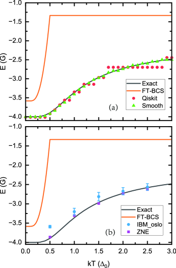
Figure 3: (a) The pairing energies of $\Omega=3$ as a function of temperatures obtained from FT-BCS and Qiskit. The original Qiskit and smoothed simulation results are shown. (b) The same pairing energies and zero-noise extrapolation (ZNE) results obtained by quantum computing.

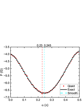
Figure 4: The simulated free energies of $\Omega=3$ as a function of variational parameters at the temperature of $kT=2.7\Delta_{0}$. The optimized variational parameters from Qiskit simulations and smoothed simulations are shown for comparison.

V. Results at Finite Temperatures

The thermal excitation states can be constructed with the eigenstates provided by zero-temperature calculations. These eigenstates are almost completely orthogonal so that an entanglement state can approximate the mixed thermal state. The exact solutions are given by the Seniority model. For comparison, the FT-BCS results which are not suitable for finite systems are also shown.

A. $\Omega=3$

For $\Omega=3$ with $N$=4 particles, the Qiskit simulations of pairing energies as a function of temperatures are shown in Fig.3. The temperature is given in the scale of $\Delta_{0}$. With the FT-BCS approximation, there is a phase transition around temperature $kT$=0.5$\Delta_{0}$ as expected, which should be smoothed out in finite systems. The ground state energy of BCS is -3.55. At high temperatures, the FT-BCS energy is -1.33 which is contributed from the Hartree term and pairing gap is vanished. We see there is a significant discrepancy between FT-BCS and exact results. The exact energies show a smooth transition as a function of temperatures. The FT-BCS results are higher than exact results both at zero and finite temperatures, since BCS includes insufficient many-body correlations. With increasing temperatures, the pairs are breaking due to thermal excitations. However, the pairs can not fully broken due to a restricted configuration space. At the limit of high temperatures, the system would have the largest entropy and eigenstates are equally mixed, and the energy limit should be -2.0 rather than -1.33 given by FT-BCS.

The false phase transition from FT-BCS demonstrated the breakdown of the BCS approximation for small systems. Note that BCS violates the conservation of particle numbers due to the breaking of U(1) symmetry. The symmetry restoration by particle number projection can improve the FT-BCS results Esebbag . However, the results of projected FT-BCS at high temperatures are close to FT-BCS Esebbag , which is not consistent with exact results of the seniority model. It is known that FT-BCS with variation after projection can well reproduce the non-degenerate pairing model lacrox3 . The energy discrepancy between exact solutions and FT-BCS at high temperatures demonstrates an analogy existence of a pseudogap pairing pseudo , i.e., a gap above $T_{c}$ is needed in Eq.(13) to account for the energy discrepancy. Here the existence of the psedogap pairing at high temperatures is due to the symmetry constraint of finite systems. This provides a clue for the origin of the pseudogap phase in high-$T_{c}$ superconductors which may be induced by specific localized symmetries. The breakdown of FT-BCS and projected FT-BCS implies the accurate treatment of many-body correlations in such small thermal-excited systems is essential.

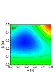
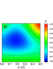
Figure 5: (a) The contour of free energies with two variational parameters by quantum simulations at $kT=2.0\Delta_{0}$ for $\Omega=4$. (b) the smoothed contour around the minima.

With Qiskit simulations, the deviations caused by statistical fluctuations are much larger at finite temperatures than at zero temperature. This is because the calculation of entropy based on wave function overlaps adds more statistical noises. In Fig.3, to reduce the noise, only one variational parameter is used considering the degeneracy of the first excited state. The original Qiskit simulations show large deviations from exact values. To this end, we applied numerical smoothing and interpolation to smooth out the statistical fluctuations. Then the smoothed results are close to exact values at finite temperatures. As an example, the variational free energy at $kT$=2.7$\Delta_{0}$ is shown in Fig.4. We see that the Qiskit simulations have small fluctuations around exact free energies. This results in small deviations in determining the variational parameter. However, the determination of pairing energies of thermal states is sensitive to these variational parameters. Thus the smoothed VQE is necessary to improve the accuracies of thermal quantum simulations.

The quantum computing results with IBM_oslo are shown in Fig.3(b). Note that in the quantum computing, the variational parameters are fixed to reduce uncertainties. We can see that the quantum computing results are slightly higher than the exact values and also demonstrate the smooth phase transition. For each temperature, we made 5 measurements and the hardware uncertainties are also shown. The earlier described error mitigation by zero-noise extrapolation is also applied at finite temperatures. The error mitigated results become close to exact values.

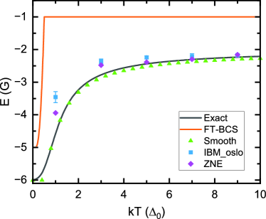
Figure 6: The pairing energies and the zero-noise extrapolation (ZNE) from quantum computing as a function of temperatures for $\Omega=4$. The FT-BCS results and exact results are shown for comparison. The smoothed simulation results by Qiskit are also shown.

B. $\Omega=4$

For $\Omega=4$, the quantum simulations at finite temperatures are more complex. We adopt two variational parameters considering the degeneracy of excited states. In principle there are 5 variational parameters but the influences of statistical noise would be very large. Fig.5 shows the Qiskit simulations of free energies with two variational parameters. We see notable fluctuations in the contour which would be difficult for VQE to determine precisely the variational parameters. Fig.5(b) shows the smoothed contour with the Fourier expansion. The smoothed VQE can also be applied to the multi-dimensional parameter space.

The thermal excitation energies of the pairing Hamiltonian of $\Omega=4$ at finite temperatures are shown in Fig.6. The FT-BCS results are also shown. It is known that the original Qiskit results have notable fluctuations in free energies. The smoothed simulations are necessary to obtain correct parameters and thus correct pairing energies. The quantum computing results and zero-noise extrapolation are shown. The zero-noise extrapolation results are satisfactory compared to exact solutions. In general, the quantum computing results of $\Omega=4$ are less accurate compared to that of $\Omega=3$. In both cases, the deviations of quantum computing become smallers with increasing temperatures, due to the cancellation between errors of different states. This is promising for quantum computing of thermal states although accumulated errors by VQD increase at higher states. For even larger systems or very high temperatures, a hybrid approach can be adopted, in which low-lying states are computed by VQD and high-lying states are computed by approximated methods such as the mean-field approximation with symmetry projections.

VI. Conclusion

We performed quantum computing of eigenstates and thermal states of the pairing Hamiltonian in a degenerate shell. For $\Omega=3$ and $\Omega=4$ with 4 particles, we show their wave functions can be simulated on 3 and 4 qubits, which correspond to much larger shell model spaces. We have applied VQD for excited states that shifts lower states out of the eigenspace successively. The quantum computing is performed with a superconducting quantum processor provided by IBM. The error mitigation of readout measurements and the zero-noise extrapolation have been demonstrated to be helpful to improve the accuracy. For $\Omega=4$, the entanglement of 6 basis on 4 qubits is realized and the circuit is constructed using the two-qubit building blocks that preserves the number of particles.

The mixed thermal state is simulated by the entanglement of the orthogonal eigenspace with the same variational circuit as at zero temperature. For comparison, the finite-temperature BCS results are also shown, which has a false phase transition from superfluid state to normal state. The quantum computing demonstrates a smooth transition as expected in finite systems. The FT-BCS is breakdown for small systems. In addition, exact results are not close to FT-BCS at high temperatures, indicating an analogy existence of pairing pseudogap. In our approach, the thermal excitations can be simulated without accurate knowledge of eigenvalues. The results from quantum computing become close to exact solutions at high temperatures. In the future, it is still desirable to develop an improved quantum algorithm to compute the entropy. The accurate treatment of many-body correlations of finite thermal systems has broad physics implications, for which quantum computing has unique opportunities.

- (1) D. S. Abrams and S. Lloyd, Phys. Rev. Lett. 83, 5162(1999)
- (2) E.F. Dumitrescu, A.J. McCaskey, G. Hagen, G.R. Jansen, T.D. Morris, T. Papenbrock, R.C. Pooser, D.J. Dean, and P. Lougovski, Phys. Rev. Lett. 120, 210501 (2018)
- (3) M. J. Cervia, A. B. Balantekin, S. N. Coppersmith, C. W. Johnson, P.J. Love, C. Poole, K. Robbins, and M. Saffman, Phys. Rev. C 104 024305 (2021)
- (4) M.Q. Hlatshwayo, Y.N. Zhang, H. Wibowo, R. LaRose, D. Lacroix, and E. Litvinova, Phys. Rev. C 106 024319 (2022)
- (5) B. Hall, A. Roggero, A. Baroni, and J. Carlson, Phys. Rev. D 104 063009 (2021)
- (6) A. Roggero, C.Y. Gu, A. Baroni, and T. Papenbrock, Phys. Rev. C 102 064624 (2020)
- (7) W. Du, J. P. Vary, X. Zhao, and W. Zuo, Phys. Rev. A 104, 012611(2021)
- (8) D. Lacroix, Phys. Rev. Lett. 125 230502 (2020)
- (9) A. L. Goodman, Nucl. Phys. A 352, 30 (1981).
- (10) Y. Alhassid, C.N. Gilbreth, and G.F. Bertsch, Phys. Rev. Lett. 113, 262503(2014)
- (11) C.Esebbag and J.L.Egido, Nucl. Phys. A 552, 205(1993)
- (12) P. Magierski, G. Wlazłowski, and A. Bulgac, Phys. Rev. Lett. 107, 145304 (2011)
- (13) T. Timusk and B. Statt, Rep. Prog. Phys. 62, 61(1999)
- (14) P. Fanto, Y. Alhassid, and G. F. Bertsch, Phys. Rev. C 96, 014305(2017)
- (15) V. Martin, J. L. Egido, and L. M. Robledo, Phys. Rev. C 68, 034327(2003)
- (16) J. C. Pei, W. Nazarewicz, J. A. Sheikh, and A. K. Kerman, Phys. Rev. Lett 102, 192501 (2009).
- (17) H. Shen, F. Ji, J.N. Hu, K. Sumiyoshi, ApJ 891, 148(2020).
- (18) A. Peruzzo, J. McClean, P. Shadbolt, M.-H. Yung, X.-Q. Zhou, P.J. Love, A. Aspuru-Guzik, and J.L. OBrien, Nat. Commun. 5, 4213 (2014).
- (19) O. Higgott, D. Wang, S. Brierley, Quantum 3, 156 (2019).
- (20) J.R. McClean, J. Romero, R. Babbush, and A. Aspuru-Guzik, New J. Phys. 18, 023023 (2016).
- (21) https://qiskit.org/
- (22) P. Jordan and E. Wigner, Z. Phys. 47, 631 (1928).
- (23) E. Ovrum and M. Hjorth-Jensen, arXiv:0705.1928v1, 2007.
- (24) A. Khamoshi, F. A. Evangelista, and G. E. Scuseria, Quantum Sci. Technol. 6, 014004 (2021).
- (25) E. A. Ruiz Guzman and D. Lacroix, Phys. Rev. C 105, 024324 (2022).
- (26) P. Ring, P. Schuck, The Nuclear Many-Body Problems, Springer(2004).
- (27) P. Kl. Barkoutsos, J. F. Gonthier, I. Sokolov, N. Moll, G. Salis, A. Fuhrer, M. Ganzhorn, D. J. Egger, M. Troyer, A. Mezzacapo, S. Filipp, and I. Tavernelli, Phys. Rev. A 98, 022322 (2018).
- (28) B. T. Gard, L. Zhu, G. S. Barron, N. J. Mayhall, S. E. Economou, and E. Barnes, NPJ Quantum Inf. 6, 10 (2020).
- (29) O. Kiss, M. Grossi, P. Lougovski, F. Sanchez, S. Vallecorsa, and T. Papenbrock, Phys. Rev. C 106, 034325(2022).
- (30) A. Aspuru-Guzik, A. D. Dutoi, P. J. Love, and M. Head-Gordon, Science 309, 1704 (2005).
- (31) M. Motta, C. Sun, A. T. K. Tan, M. J. O’Rourke, E. Ye, A. J. Minnich, F. G. S. L. Brandao, and G. K.-L. Chan, Nature Physics 16, 205 (2020).
- (32) P. J. Ollitrault, A. Kandala, C.-F. Chen, P. K. Barkoutsos, A. Mezzacapo, M. Pistoia, S. Sheldon, S. Woerner, J. M. Gambetta, and I. Tavernelli, Phys. Rev. Res. 2, 043140 (2020).
- (33) E. Khan, N.Van Giai, N. Sandulescu, Nucl. Phys. A 789, 94(2007).
- (34) J. Wu, and T. H. Hsieh, Phys. Rev. Lett. 123, 220502(2019).
- (35) M. Motta, C. Sun, A. T. K. Tan, M. J. ORourke, E. Ye, A. J. Minnich, F. G. S. L. Brandão and G. Kin-Lic Chan, Nature Phys. 16, 205(2020)
- (36) A. Francis, D. Zhu, C. H. Alderete, S. Johri, X. Xiao, J. K. Freericks, C. Monroe, N. M. Linke, A. F. Kemper, Sci. Adv. 7, eabf2447(2021)
- (37) I. Stetcu, A. Baroni, and J. Carlson, Phys. Rev. C 105, 064308 (2022).
- (38) W. H. Press, S. A. Teukolsky, W. T. Vetterling, B. P. Flannery, Numerical Recipes, (Cambridge University Press, UK, 2007).
- (39) N. Klco, E. F. Dumitrescu, A. J. McCaskey, T. D. Morris, R. C. Pooser, M. Sanz, E. Solano, P. Lougovski, and M. J. Savage, Phys. Rev. A 98, 032331(2018)
- (40) D. Gambacurta and D. Lacroix, Phys. Rev. C 85, 044321(2012)