DAG: Depth-Aware Guidance with Denoising Diffusion Probabilistic Models

Abstract

Generative models have recently undergone significant advancement due to the diffusion models. The success of these models can be often attributed to their use of guidance techniques, such as classifier or classifier-free guidance, which provide effective mechanisms to trade-off between fidelity and diversity. However, these methods are not capable of guiding a generated image to be aware of its geometric configuration, e.g., depth, which hinders their application to areas that require a certain level of depth awareness. To address this limitation, we propose a novel guidance method for diffusion models that uses estimated depth information derived from the rich intermediate representations of diffusion models. We first present label-efficient depth estimation framework using internal representations of diffusion models. Subsequently, we propose the incorporation of two guidance techniques based on pseudo-labeling and depth-domain diffusion prior during the sampling phase to self-condition the generated image using the estimated depth map. Experiments and comprehensive ablation studies demonstrate the effectiveness of our method in guiding the diffusion models towards the generation of geometrically plausible images.

Korea University, Seoul, Korea
{kkn9975,jws1997,jpl358,susung1999,se780,seungryong_kim}@korea.ac.kr

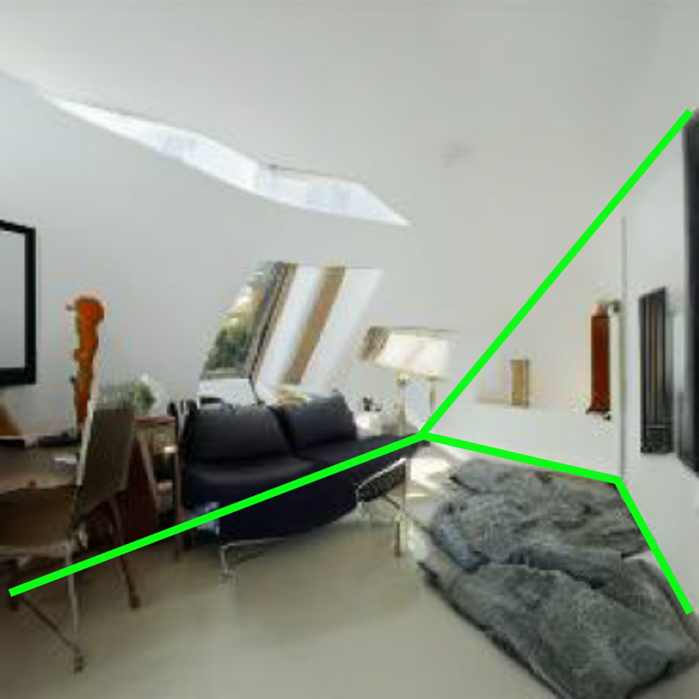
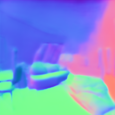
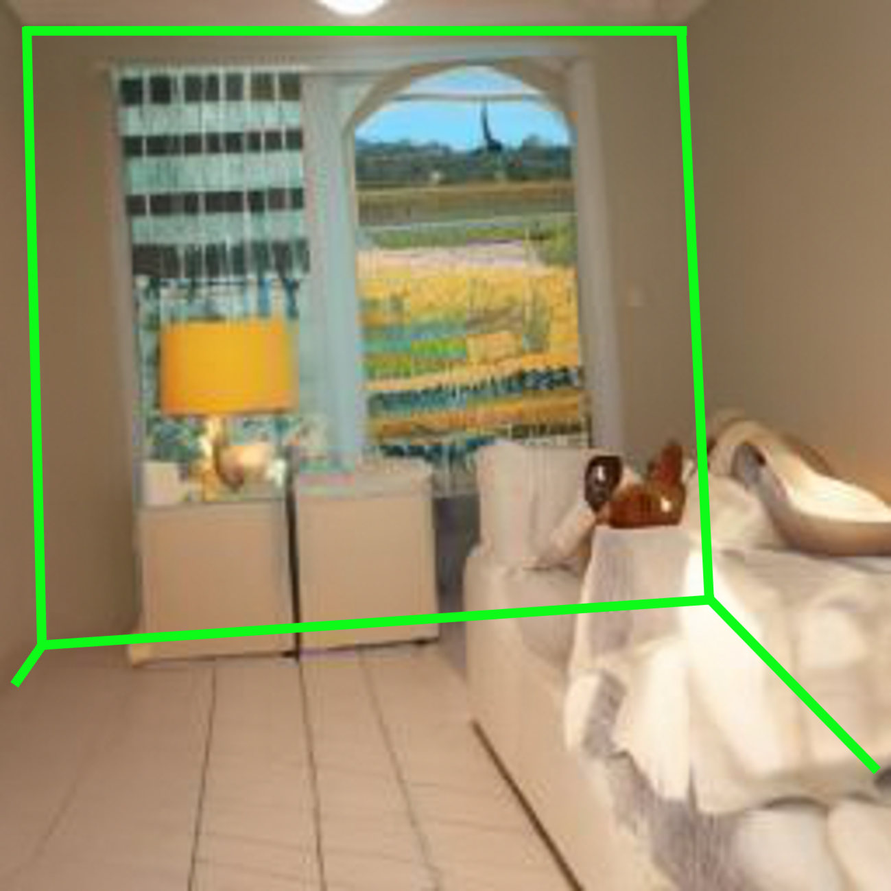
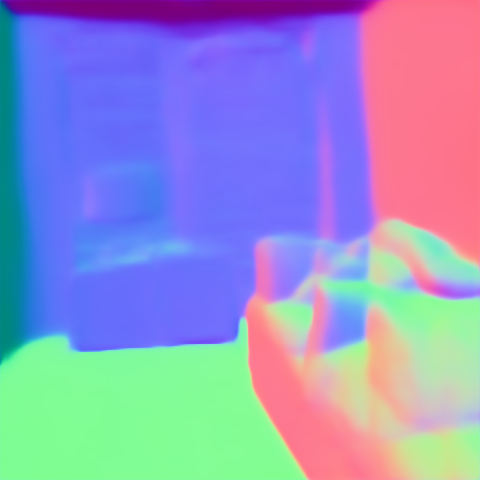
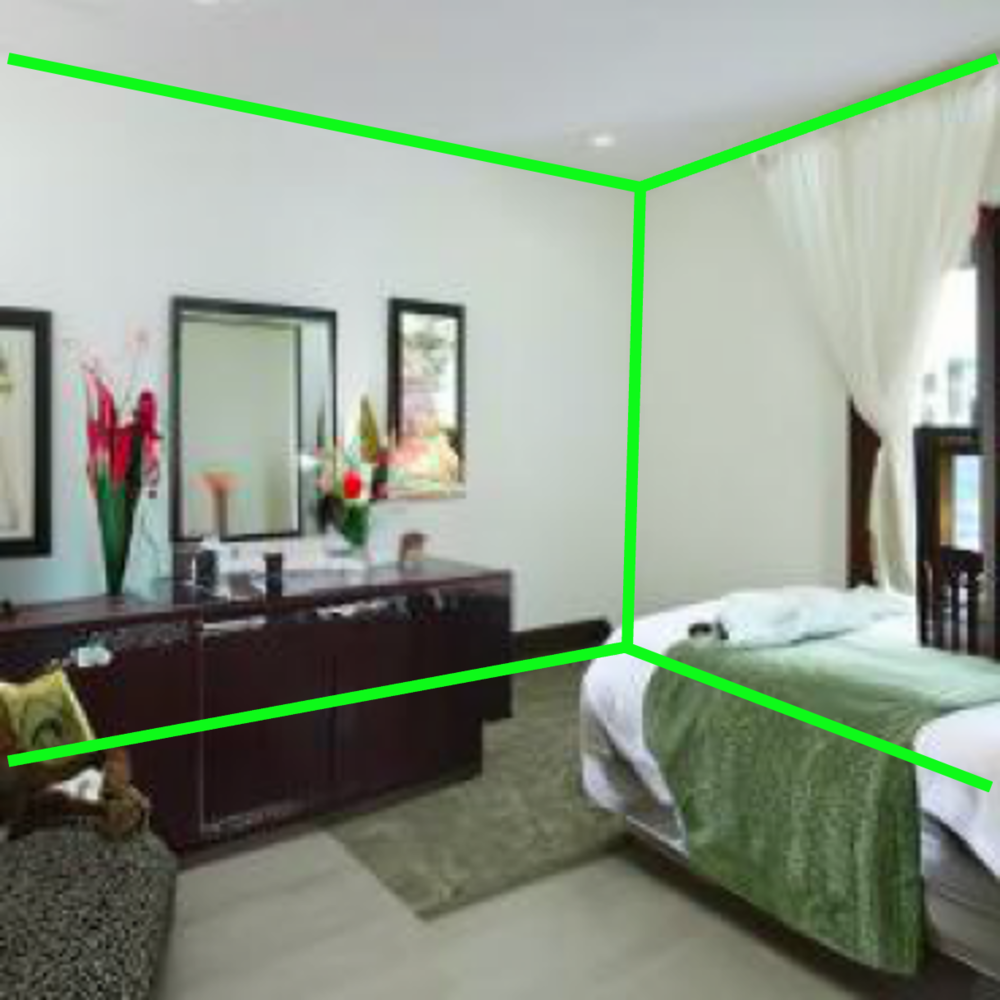
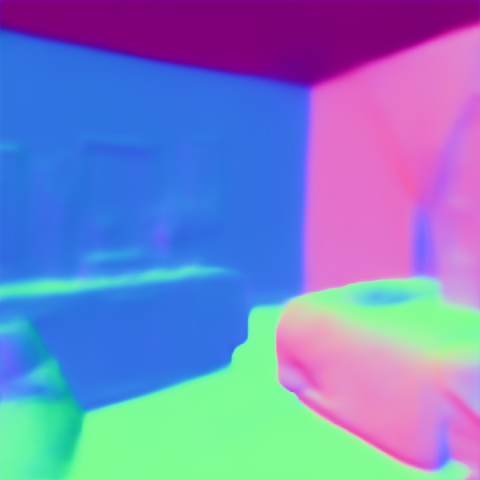
Figure 1: Qualitative comparisons of synthesized images without guidance (Dhariwal & Nichol, 2021) (top) and with our depth-aware guidance (DAG), and their corresponding estimated depths (Ranftl et al., 2021) and surface normals (Bae et al., 2021). Note that we highlight the scene layouts on the generated images. Our DAG helps better generate geometrically plausible images compared to the baseline (Dhariwal & Nichol, 2021).

1 Introduction

Diffusion models (Sohl-Dickstein et al., 2015; Ho et al., 2020; Nichol & Dhariwal, 2021; Rombach et al., 2022) have recently received much attention and have shown remarkable generation quality. Such superior performance of diffusion models promoted many applications, such as text-guided image synthesis (Nichol et al., 2021; Ramesh et al., 2022), image restoration (Saharia et al., 2022c, a; Kawar et al., 2022) and semantic segmentation (Baranchuk et al., 2022; Asiedu et al., 2022).

Generally, generative models (Goodfellow et al., 2020; Ho et al., 2020; Farid, 2022), especially diffusion models, focus primarily on texture or appearance (Tewari et al., 2022) but hardly consider shape geometry during the image generation process. As a result, as demonstrated in Fig. 1, conventional diffusion models often generate geometrically implausible images that contain ambiguous depth and cluttered object layouts. These synthesized samples with such unrealistic 3D geometry, whose deviation can be effectively captured by the depth map in 2D, are problematic in that they are not only visually unappealing but also unsuitable for downstream tasks, e.g., robotics and autonomous driving (Wang et al., 2019; Tateno et al., 2017).

While there have been some class-conditional guidance approaches (Dhariwal & Nichol, 2021; Ho & Salimans, 2021) that drive the sampling process of diffusion models to a class-specific distribution, guiding the samples towards a geometrically plausible image distribution has received limited attention. In light of this, we propose a novel framework called Depth-Aware Guidance (DAG) that introduces depth awareness to diffusion models. Training diffusion models or depth predictors from scratch with depth-image pairs, as in conventional guidance (Dhariwal & Nichol, 2021; Ho & Salimans, 2021), can be challenging because it requires a lot of effort to annotate the ground-truth depth map and it takes tremendous time and computations to jointly train the models. To overcome these challenges, we employ a novel approach by utilizing the rich representations of a pretrained diffusion model to train depth predictors for the first time, thereby extending the knowledge of the representation capabilities of diffusion models in depth prediction tasks.

Furthermore, by leveraging label-efficient depth predictors, we propose a depth-aware guidance approach for image generation with the diffusion model. Specifically, we present two guidance strategies that effectively guide the geometric awareness: depth consistency guidance and depth prior guidance. The first strategy, depth consistency guidance, is motivated by consistency regularization (Bachman et al., 2014; Sajjadi et al., 2016; Laine & Aila, 2016). By treating the better prediction as a depth pseudo-label, depth consistency guidance guides the image toward improving the poor prediction. The second strategy, depth prior guidance, utilizes an additional pretrained diffusion U-Net as a prior network (Graikos et al., 2022; Poole et al., 2022) to provide guidance during the sampling process. This design explicitly injects depth information into the sampling process of diffusion models.

To evaluate our framework, we conduct experiments on indoor and outdoor scene datasets (Yu et al., 2015; Nathan Silberman & Fergus, 2012) and propose new metric from the perspective of depth estimation tasks to capture geometric awareness. Our results, both qualitative and quantitative, demonstrate the superiority of our approach, and our extensive ablation studies validate its effectiveness. To the best of our knowledge, our work is the first attempt to utilize depth information during the sampling process to make image generation more aware of geometric configuration.

To sum up, we present the following key contributions:

• We investigate the depth information contained in the learned U-Net representations of diffusion models.

• Based on the investigation, we propose a novel framework that can impose depth awareness of images generated from diffusion models.

• The training of depth predictors in this framework can be done in a label-efficient manner by piggybacking on pretrained diffusion models.

• We propose novel guidance strategies that make use of consistency regularization and depth prior.

2 Related Work

Denoising diffusion probabilistic models.

Diffusion models (Sohl-Dickstein et al., 2015; Ho et al., 2020), as the name states, model the reverse diffusion process, which gradually removes Gaussian noise from the latent variable. (Song et al., 2020) have shown that diffusion models are equivalent to score-based generative models via stochastic differential equation interpretation. These models allow us to generate images from a complete Gaussian noise. Various attempts have been made to enhance the sample quality and sampling speed through different approaches (Nichol & Dhariwal, 2021; Hong et al., 2022; Dhariwal & Nichol, 2021; Rombach et al., 2022; Song et al., 2021). (Nichol & Dhariwal, 2021) estimated the variance of reverse diffusion process and (Dhariwal & Nichol, 2021) searched for an optimal U-shaped architecture for better sampling quality. (Song et al., 2021) proposed non-Markovian diffusion process to reduce sampling steps whereas (Rombach et al., 2022) leveraged diffusion process in the discrete latent space introduced in (Esser et al., 2020) for efficient computation and faster sampling. As a result of this advancement, diffusion models now outperform previous state-of-the-art models in various image generation tasks (Nichol et al., 2021; Seo et al., 2022; Saharia et al., 2022b; Ramesh et al., 2022; Rombach et al., 2022; Choi et al., 2021). Additionally, text-to-image diffusion models (Rombach et al., 2022; Saharia et al., 2022b; Balaji et al., 2022) have been utilized as a strong image prior for text-to-3D generation (Poole et al., 2022; Lin et al., 2022) in recent studies.

Sampling guidance for diffusion models.

(Dhariwal & Nichol, 2021) first proposed classifier guidance that leverages the gradient of an external classifier during the sampling process. By scaling the gradient, we can control the trade-off between the fidelity and diversity of the generated images. As an alternative without needing an external classifier, classifier-free guidance (Ho & Salimans, 2021) has been proposed. During training, they randomly drop a certain percentage of class labels to obtain both conditional and unconditional models with shared parameters. With these two models, they get a similar effect on the classifier guidance. Applying these guidance leads to significant development in a conditional generation like text-to-image generation (Nichol et al., 2021; Rombach et al., 2022; Saharia et al., 2022b; Ramesh et al., 2022; Gu et al., 2022) and semantic map-guided image generation (Wang et al., 2022b, a). However, to our best knowledge, guidance for sampling with geometric awareness has been unexplored.

Internal representations in diffusion models.

Recent studies (Baranchuk et al., 2022; Asiedu et al., 2022) have also analyzed and utilized the intermediate U-Net representations of diffusion models. (Baranchuk et al., 2022) demonstrated that the U-Net representations of diffusion models at different layers contain semantic contexts of images and can predict semantic segmentation maps using only a shallow MLP and a scarcely-labeled dataset. Also, (Asiedu et al., 2022) found similar phenomena that decoder pretraining of recovering the noised image like denoising autoencoders (Vincent et al., 2008) achieves high performance in label-efficient semantic segmentation task. For the first time, we propose to capture depth information using internal representations.

Monocular depth estimation.

Monocular depth estimation, which aims to estimate a dense depth map from a single image (Eigen et al., 2014; Li et al., 2015; Wang et al., 2015; Kim et al., 2016; Ummenhofer et al., 2017), is an essential component of 3D perception. Since (Eigen et al., 2014) proposed a deep learning-based approach for this task, several works (Lee et al., 2019; Laina et al., 2016; Fu et al., 2018) have achieved significant progress due to the ability of CNNs to learn strong priors from images corresponding to the geometric layout. Following the recent success of Transformer (Dosovitskiy et al., 2020; Vaswani et al., 2017) in vision tasks, (Ranftl et al., 2021; Bhat et al., 2021; Li et al., 2022) employed a Transformer-based encoder to exploit a global receptive field. Despite notable improvements, recent works increase the model complexity and the reliance on large paired supervision.

3 Preliminaries

Denoising diffusion probabilistic models.

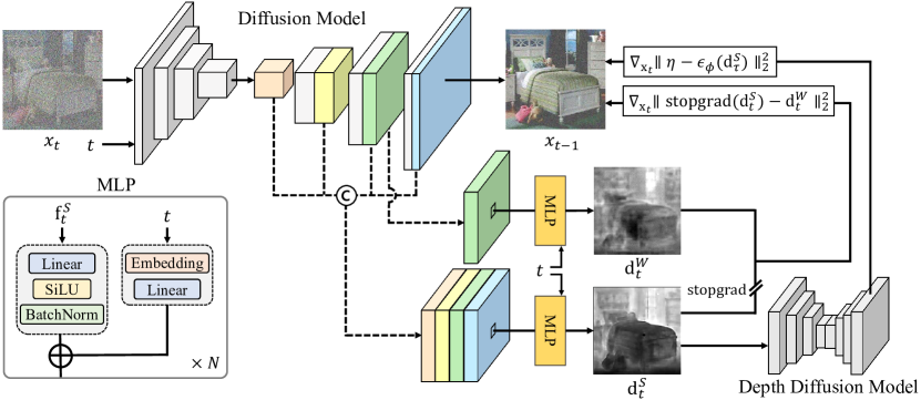
Figure 2: Overview of our framework. First of all, we train asymmetric pixel-wise depth predictor conditioned on a timestep with respect to pretrained diffusion models in a label-efficient manner. Then, we apply two guidance strategies. First, we extract strong and weak depth maps with this predictor from DDPM network and give a depth consistency guidance. Next, giving the depth map from the strong branch as an input, the pretrained depth diffusion model is utilized to push the model prior into intermediate images to be depth-aware.

DDPM (Ho et al., 2020) is a kind of generative model that generates an image by iteratively denoising from Gaussian noise. In specific, given an input image $\mathbf{x}_{0}$ and an input noise $\epsilon\sim\mathcal{N}(\mathbf{0},\mathbf{I})$, DDPM gradually adds noise according to a timestep $t$. For a pre-defined variance schedule $\beta_{t}$ for $t\in\{T,T-1,\ldots,1\}$, we denote $\alpha_{t}$ and $\bar{\alpha}_{t}$ as $1-\beta_{t}$ and $\Pi^{t}_{k=1}\alpha_{k}$, respectively. Then, given an arbitrary $t$, the forward process can be expressed in closed form (Ho et al., 2020):

$$\mathbf{x}_{t}=\sqrt{\bar{\alpha}_{t}}\mathbf{x}_{0}+\sqrt{1-\bar{\alpha}_{t}}\mathbf{\epsilon}.$$ (1)

As noted in Ho et al. (Ho et al., 2020), we can re-weight the training objective of DDPM as:

$$\mathcal{L}_{\mathrm{simple}}=\|\epsilon-\epsilon_{\theta}(\mathbf{x}_{t})\|_{2}^{2},$$ (2)

where $\epsilon_{\theta}$ is a denoising U-Net (Ho et al., 2020) parameterized with $\theta$. Subsequently, the sampling process of DDPM is defined as the reverse of the forward process:

$$\mathbf{x}_{t-1}\sim\mathcal{N}(\mu_{\theta}(\mathbf{x}_{t}),\sigma_{t}^{2}),$$ (3)

where $\sigma_{t}^{2}$ is a constant only dependent on $t$, and $\mu_{\theta}$ is a prediction of the mean computed from the reparameterization of $\epsilon_{\theta}$. In some works (Nichol & Dhariwal, 2021; Dhariwal & Nichol, 2021), the variance is also predicted and then Eq. 3 turns into:

$$\mathbf{x}_{t-1}\sim\mathcal{N}(\mu_{\theta}(\mathbf{x}_{t}),\Sigma_{\theta}(\mathbf{x}_{t})),$$ (4)

where $\Sigma_{\theta}$ is a prediction of variance in the reverse process from the model output. To formulate the task as conditional image generation with diffusion models, the need for guidance method is increasing.

Classifier guidance for diffusion model.

By providing a way to trade off diversity and fidelity, classifier guidance (Dhariwal & Nichol, 2021) can improve the sample quality for image synthesis tasks. For a trained classifier $p_{\psi}(\mathbf{y}|\mathbf{x}_{t})$, which receives the noised image $\mathbf{x}_{t}$ and predicts the class $\mathbf{y}$, a gradient with respect to $\mathbf{x}_{t}$ is calculated as:

$$\nabla_{\mathbf{x}_{t}}\log(p_{\psi}(\mathbf{y}|\mathbf{x}_{t})).$$ (5)

Then, the sampling process with classifier guidance is defined as follows:

$$\mathbf{x}_{t-1}\sim\mathcal{N}(\mu_{\theta}(\mathbf{x}_{t})+w\Sigma\nabla_{\mathbf{x}_{t}}\log(p_{\psi}(\mathbf{y}|\mathbf{x}_{t})),\Sigma_{\theta}(\mathbf{x}_{t})).$$ (6)

where $w>0$ is a scale of guidance.

Even though this technique improves the sampling quality, no studies have attempted to extend it by leveraging dense predictors that incorporate geometric awareness.

4 Methodology

4.1 Motivation and Overview

Although the synthesized images by existing generative models such as GANs (Goodfellow et al., 2014) or diffusion models (Sohl-Dickstein et al., 2015; Ho et al., 2020) seem to be fairly plausible, they often lack geometric awareness. For example, the generated images by the existing models (Farid, 2022) often contain out-of-perspective or distortion of the layout, as depicted in Fig. 5. This failure of considering geometric awareness can be an obstacle when applied to many downstream tasks (Lin et al., 2013; Tateno et al., 2017) that require geometrically realistic images.

To overcome this limitation, we propose a novel framework, illustrated in Fig. 2, to explicitly incorporate geometric information into the diffusion model as guidance. Specifically, to generate depth-aware images, we train depth predictors using internal representation (Baranchuk et al., 2022) with a small amount of depth-labeled data. Then, we guide the intermediate images using obtained depth map during the sampling process.

In Sec. 4.2, we demonstrate a way to acquire a depth map in a label-efficient way, and in Sec. 4.3, we propose sampling methods to guide the generated images to have depth awareness.

4.2 Label-Efficient Training of Depth Predictors

In order to generate depth-aware images with diffusion guidance in a straightforward way as in  (Dhariwal & Nichol, 2021), we need either a large amount of image-depth pairs or an external large-scale depth estimation network trained on the noised images, both of which are challenging to acquire. To address this problem, we re-use the rich representations learned with DDPM that may contain depth information of images to estimate the depth.

Network architecture.

Recent research has shown that the internal features of the networks trained with diffusion models can encode semantic information (Vincent et al., 2008; Baranchuk et al., 2022; Asiedu et al., 2022), and our contribution builds upon this by incorporating depth information into the framework.

To perform depth estimation in a label-efficient manner, we utilize a pixel-wise shallow Multi-Layer Perceptron (MLP) regressor that receives intermediate features from U-Net and estimates the depth values of the noisy input image. Specifically, we acquire the internal features $\mathbf{f}_{t}(k)\in\mathbb{R}^{C(k)\times H(k)\times W(k)}$ from the output of $k$-th decoder layer in the diffusion U-Net, where $C(k)$ denotes the channel dimension and $H(k)\times W(k)$ denotes the spatial resolution of the $k$-th layer of the U-Net decoder. Subsequently, we form the depth map by querying the MLP blocks pixel-by-pixel, where the depth map can be formulated as:

$$\mathbf{d}_{t}(k)=\text{MLP}(\mathbf{f}_{t}(k)).$$ (7)

Also, similar to (Baranchuk et al., 2022), it is generally better to use more features from different U-Net layers than only using the feature from one layer. Therefore we extract more features from many layers and concatenate them in a channel dimension, which can be formulated as:

$$\mathbf{g}_{t}=[\mathbf{f}_{t}(1);\mathbf{f}_{t}(2);\cdots;\mathbf{f}_{t}(d)],$$ (8)

where $[\cdot\,;\cdot]$ is a channel-wise concatenation operation between features, and $d$ is the total number of selected layers. Then, we pass them to the pixel-wise MLP depth predictor, and the generalization of Eq. 7 in terms of Eq. 8 can be stated as:

$$\mathbf{d}_{t}=\text{MLP}(\mathbf{g}_{t}).$$ (9)

We modify the pixel-wise depth predictor by appending an additional time-embedding block to the input in order to predict the depth map at arbitrary timesteps. Therefore, we can use this predictor throughout the entire sampling process. We follow the time-embedding module of diffusion U-Net. Applying it to Eq. 7, we can rewrite the equation as:

$$\mathbf{d}_{t}=\text{MLP}(\mathbf{g}_{t},t).$$ (10)

$t$=800	$t$=600	$t$=400	$t$=200	$t$=0

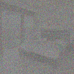
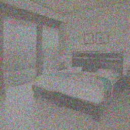
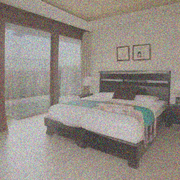
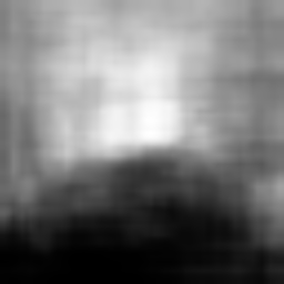
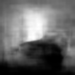
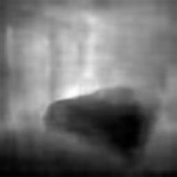
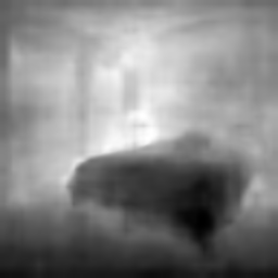
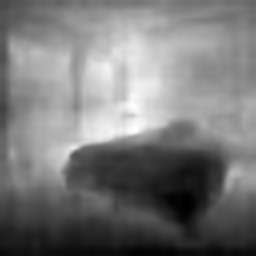
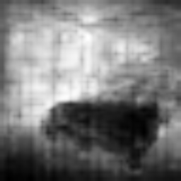
Figure 3: Visualizations of the sampling process of our framework: (from top to bottom) predicted images, depth predictions from the strong-branch predictor ($\mathbf{d}^{S}_{t}$), and depth predictions from the weak-branch predictor ($\mathbf{d}^{W}_{t}$). As exemplified, the strong-branch predictor gives robust depth predictions even at the early stage.

Loss function.

We train the depth estimator only with the frozen features from the diffusion U-Net by using the ground-truth depth map $\mathbf{y}$ with L1 loss as

$$\mathcal{L}_{\mathrm{depth}}=\|\mathbf{d}_{t}-\mathbf{y}\|_{1}.$$ (11)

This whole procedure allows us to achieve reasonable label-efficient prediction performance in the depth domain, as demonstrated in Fig. 4(b). The depth prediction scheme allows us to predict the depth map not only for any input images but also for the intermediate images under generation in arbitrary sampling steps, as shown in Fig. 3, since the representations of diffusion models are inherently learned with the timesteps.

4.3 Depth Guided Sampling for Diffusion Model

To ensure that the generated images yield plausible depth maps, we encourage the predicted depth maps to be accurate during the sampling process. To this end, we propose two different guidance techniques that use the representations of the denoising U-Net. Utilizing these techniques during the sampling process regularizes the model to generate images that are aware of the dense map prior. Specifically, we use the aforementioned efficiently-trained depth predictors in Sec. 4.2, which can predict the depth maps from images at any sampling steps.

Unfortunately, because of the absence of a pre-determined label, we cannot compute loss using this label and cannot give guidance during the sampling process. Therefore we build two alternative loss functions that can act as guidance constraints, which we discuss in detail in the following sections. Considering Eq. 6, The general form of guidance equation is formulated by:

$$\mathbf{x}_{t-1}\sim\mathcal{N}(\mu_{\theta}(\mathbf{x}_{t})-\omega\nabla_{\mathbf{x}_{t}}{\mathcal{L}_{\mathrm{depth}}},\Sigma_{\theta}(\mathbf{x}_{t})).$$ (12)

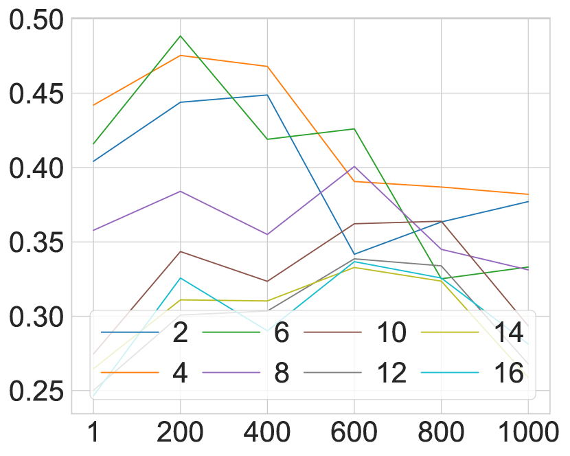
(a)

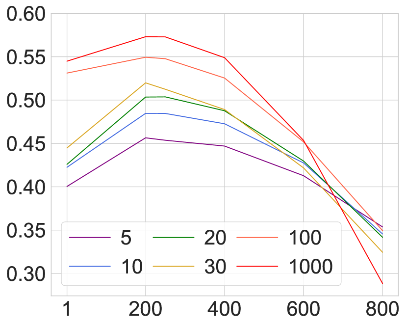
(b)

Figure 4: Quantitative comparisons of depth prediction performance. Evaluation of depth estimation performance for varying timesteps according to different U-Net blocks and the number of training images. The x-axis denotes timesteps and the y-axis denotes the accuracy of depth estimation. (a) Comparison of depth prediction accuracy according to different U-Net blocks. Each line denotes the layer from which the feature map is extracted in the decoder of U-Net. (b) Comparison of depth prediction accuracy with the number of images shown in training. For (b), each line denotes the number of samples shown.

Depth consistency guidance (DCG).

One naive approach for providing depth guidance to the images in the absence of ground truth depth information is to use pseudo-labeling (Sohn et al., 2020; Lee et al., 2013). However, it is challenging to generate a confident prediction that can be pseudo-label. Our first guidance method is inspired by FixMatch (Sohn et al., 2020), which combines pseudo-labeling (Lee et al., 2013) and consistency regularization (Bachman et al., 2014; Sajjadi et al., 2016). It boosts performance by considering the weakly-augmented labels as pseudo-label. Our hypothesis derives from this design: we argue that the richer the representation is, the more faithful produced depth map becomes. Therefore, we regard the predictions from the aggregation of more feature blocks to be more informative, which makes them suitable to be treated as robust predictions (Fig. 3), i.e., pseudo-labels. We refer to these predictions that use multiple feature blocks as ”strong branch predictions”, and those that utilize relatively fewer features as ”weak branch predictions”.

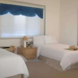
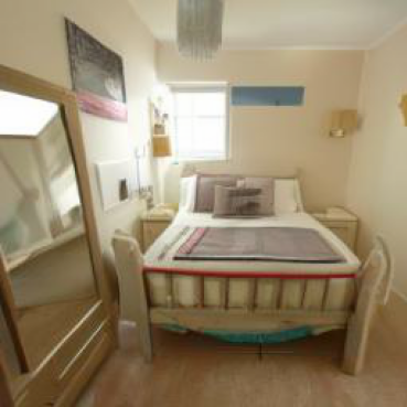
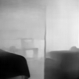
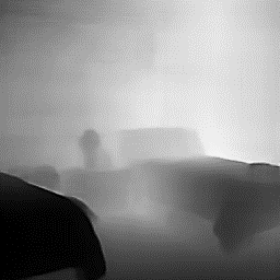
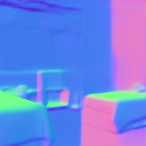
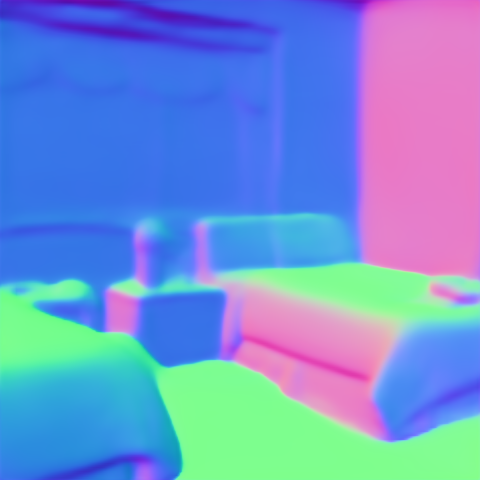
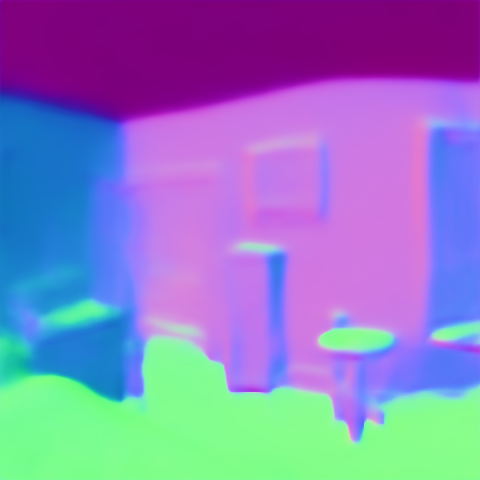
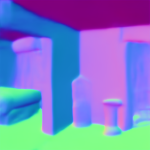
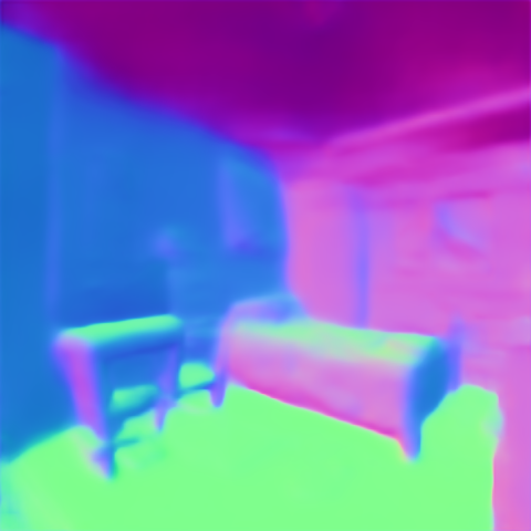
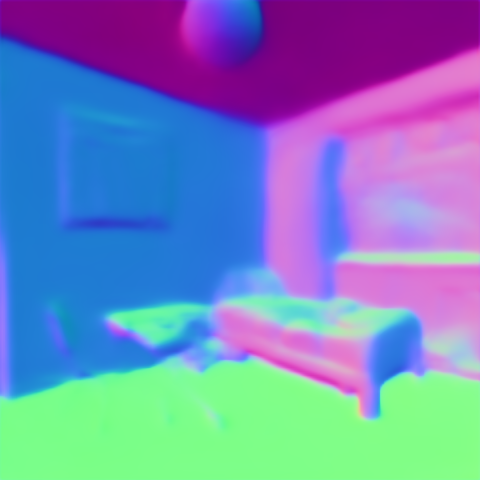
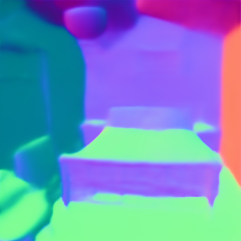
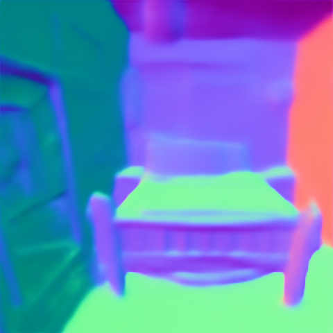
(a)	(b)	(c)	(d)	(e)	(f)	(g)	(h)

Figure 5: Qualitative comparison on LSUN bedroom datasets (Yu et al., 2015). We visualize the generated images (top) without guidance ((a), (c), (e), (g)) and with depth-aware guidance ((b), (d), (f), (h)), and their corresponding depths (Ranftl et al., 2021) (middle) and surface normals (Bae et al., 2021) (bottom).

In specific, we use the features $\mathbf{g}^{W}=[\mathbf{f}_{t}(6)]$ for weak branch features, and $\mathbf{g}^{S}=[\mathbf{f}_{t}(2);\mathbf{f}_{t}(4);\mathbf{f}_{t}(5);\mathbf{f}_{t}(6);\mathbf{f}_{t}(7)]$ for strong branch features. To account for the different channel dimensions of these two aggregated features, we design two asymmetric predictors: MLP-S and MLP-W. The first predictor receives more features from the U-Net block, while the second one receives fewer features, and we train them together. We feed the collected features to these MLPs and obtain the depth map predictions:

$$\mathbf{d}^{S}_{t}=\text{MLP-S}(\mathbf{g}^{S}_{t},t),\quad\mathbf{d}^{W}_{t}=\text{MLP-W}(\mathbf{g}^{W}_{t},t).$$ (13)

As stated above, we treat $\mathbf{d}^{S}_{t}$ as a pseudo-label and $\mathbf{d}^{W}_{t}$ as a prediction then compute the loss using a consistency loss between two predicted dense maps. We apply the stop-gradient operation to the strong features, preventing the strong prediction from learning the weak prediction (Chen & He, 2021; Sohn et al., 2020). The gradient of the loss with respect to $\mathbf{x}$ flows through the diffusion U-Net and guides the sampling process as done in (Dhariwal & Nichol, 2021). This process can be formulated as

$$\mathcal{L}_{\mathrm{dc}}=\|\mathrm{stopgrad}(\mathbf{d}^{S}_{t})-\mathbf{d}^{W}_{t}\|^{2}_{2},$$ (14)

where $\mathrm{stopgrad}$ denotes the stop-gradient operation.

Finally, we can guide the generation process by using this gradient with Eq. 12, and it can be formulated as:

$$\mathbf{x}_{t-1}\sim\mathcal{N}(\mu_{\theta}(\mathbf{x}_{t})-\omega_{\mathrm{dc}}\nabla_{\mathbf{x}_{t}}{\mathcal{L}_{\mathrm{dc}}},\Sigma_{\theta}(\mathbf{x}_{t})),$$ (15)

where $\omega_{\mathrm{dc}}$ denotes the guidance scale.

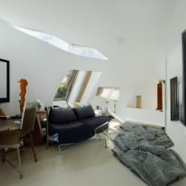
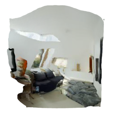
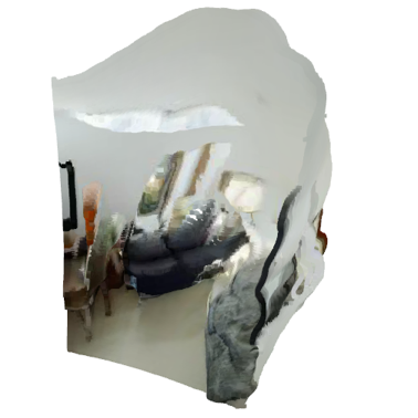
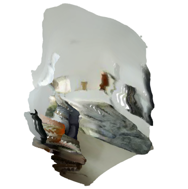
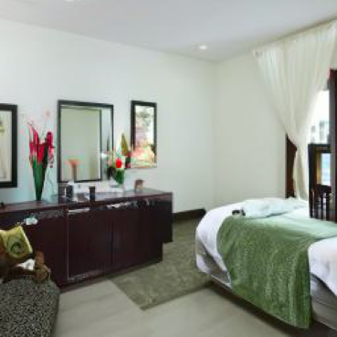
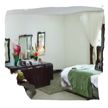
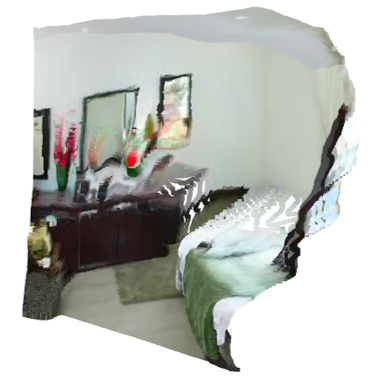
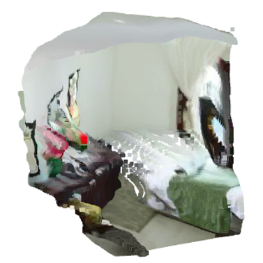
(a) (a)

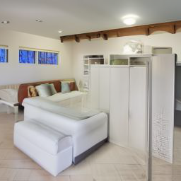
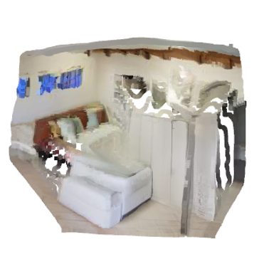
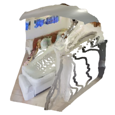
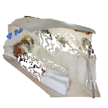
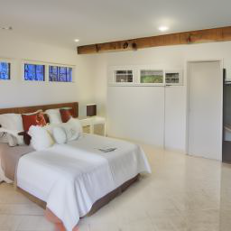
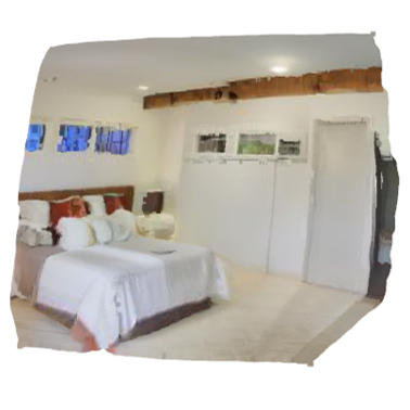
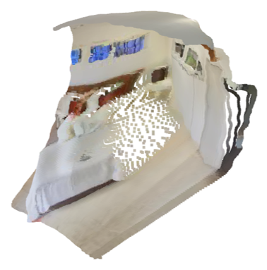
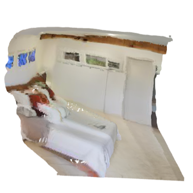
(b) (b)

Figure 6: Visualization of point cloud representation obtained by depth information. We compare the results generated from the baseline without (top) and with (bottom) our guidance by showing images and converting them into point cloud visualizations in four different views.

Depth prior guidance (DPG).

We also propose another guidance method, which we call depth prior guidance, to inject depth prior into the sampling process. The pretrained diffusion model can effectively refine the noised distributions to realistic distributions (Meng et al., 2021), or it can help to optimize the noised initialization of the data to match with the real data by utilizing the knowledge of the diffusion model (Graikos et al., 2022; Poole et al., 2022). Therefore we train another small-resolution diffusion U-Net $\epsilon_{\phi}$ on the depth domain and use it as our prior for the second guidance method. As described in Sec. 4.2, we can extract the features from the decoder part of the image-generating U-Net to estimate the corresponding depth map using MLP depth predictor. Utilizing the prior diffusion model, we inject noise to the depth prediction $\mathbf{d}^{S}_{0}$ using a forward process of diffusion like:

$$\mathbf{d}^{S}_{\tau}=\sqrt{\bar{\alpha}_{\tau}}\mathbf{d}^{S}_{0}+\sqrt{1-\bar{\alpha}_{\tau}}\eta,\quad\eta\sim\mathcal{N}(\mathbf{0},\mathbf{I}),$$ (16)

where $\tau$ is the timestep that is used in a prior diffusion model. After adding noise to the depth prediction, we feed it to our prior network to estimate the added noise. Then we calculate the gradient of the mean-squared error between the added noise and the predicted noise concerning $x$. This process is then defined as:

$$\mathcal{L}_{\mathrm{dp}}=\|\eta-\epsilon_{\phi}(\mathbf{d}^{S}_{\tau}))\|^{2}_{2}.$$ (17)

Treating the gradient of the above loss as an external classifier gradient like (Dhariwal & Nichol, 2021), we can guide the generated image to match with the depth prior like:

$$\mathbf{x}_{t-1}\sim\mathcal{N}(\mu_{\theta}(\mathbf{x}_{t})-\omega_{\mathrm{dp}}\nabla_{\mathbf{x}_{t}}\mathcal{L}_{\mathrm{dp}},\Sigma_{\theta}(\mathbf{x}_{t})),$$ (18)

where $\omega_{\mathrm{dp}}$ denotes the guidance scale.

Overall guidance.

By integrating the proposed DCG and DPG, we can guide the sampled image using both. Using Eq. 15 and 18, our overall sampling can be written as:

$$\mathbf{x}_{t-1}\sim\mathcal{N}(\mu_{\theta}(\mathbf{x}_{t})-\omega_{\mathrm{dc}}\nabla_{\mathbf{x}_{t}}{\mathcal{L}_{\mathrm{dc}}}-\omega_{\mathrm{dp}}\nabla_{\mathbf{x}_{t}}\mathcal{L}_{\mathrm{dp}},\Sigma_{\theta}(\mathbf{x}_{t})).$$ (19)

5 Experiments

5.1 Experimental Settings

Datasets.

In order to evaluate the performance of our proposed method, we conduct experiments on LSUN-Bedroom and LSUN-Church (Yu et al., 2015) for both depth estimation and image generation tasks. These datasets have been chosen to demonstrate depth-aware image synthesis in indoor and outdoor scenes, respectively. As there are no ground-truth depth labels available in the LSUN dataset, we generate pseudo-labels using a DPT (Ranftl et al., 2021) pretrained on the NYU-Depth dataset (Silberman et al., 2012) and utilize them for training the depth estimator.

Implementation details.

We base our experiment on the label-efficient framework presented in (Baranchuk et al., 2022), where we modify the architecture of the pixel classifier to model a depth estimator. We use the pretrained weights from ADM (Dhariwal & Nichol, 2021) for LSUN-Bedroom, and for LSUN-Church, we build upon the publicly available repository of DDIM (Song et al., 2021) and Diffusers library (von Platen et al., 2022). We use Adam optimizer (Kingma & Ba, 2014) to train the depth predictor MLP, and for the sampling of the diffusion model, we employ the DDIM sampler with a DDIM25 scheduler provided in the official repository of ADM (Dhariwal & Nichol, 2021) and DDIM. More detailed hyper-parameters and settings can be found in the appendix.

Evaluation metrics for depth-awareness.

Our primary contribution is the incorporation of geometric awareness in the image generation process, which is not reflected by the performance metrics commonly used in the image domain. Therefore, we introduce a novel performance metric for models that generate depth-guided images. First, we predict the depth maps of generated images using Dense Prediction Transformer (DPT) (Ranftl et al., 2021), a state-of-the-art monocular depth estimator. To measure the reality of the depth estimation map, we directly evaluate FID (Shi et al., 2022) with depth images and denote it dFID. To make a fair comparison, we build the reference batch following (Dhariwal & Nichol, 2021) with the depth predictions of images from the dataset with DPT-Hybrid.

Table 1: Quantitative Results on the LSUN-bedroom (Yu et al., 2015) dataset. dFID denotes the FID score using the estimated depth image. The metrics are computed with 5,000 generated samples. The best result is in bold.

Methods	DPG	DCG	dFID ($\downarrow$)
Baseline	-	-	15.71
DAG	✓	-	14.18
	-	✓	15.27
	✓	✓	13.93

5.2 Experimental Results

Depth prediction performance.

First, to guide the diffusion sampling process using the depth predictor, we must validate its performance according to varying training dataset sizes, feature blocks, and timesteps. To provide guidance for synthesizing images at nearly all timesteps, we train the predictor for timesteps $t<800$. This is due to our observation that the depth predictions at $t\geq 800$ do not have any useful information. We evaluate the depth performance using the depth accuracy metric ($\delta<1.25$), and the results are shown in Fig. 4. Based on the results in Fig. 4 (a), we choose to use the middle feature blocks $\{l_{n}\}=\{2,4,5,6,7\}$, which show relatively high accuracy. In DCG, we also choose the feature maps by sorting the layer by accuracy, and the result is $S=\{2,4,5,6,7\}$ and $W=\{6\}$. Next, Fig. 4 (b) illustrates the depth prediction accuracy with respect to the number of training images and evaluated timesteps. To minimize the sampling variance, We report the mean from a total of 10-fold training results. As the training data size increases, the performance of the model shows improvement accordingly. When trained with 1,000 images, the model achieves the highest accuracy. However, the performance increase compared to the 100-label setting is marginal, so we choose to use 100 images for training the depth predictor.

Quantitative results.

We compare the results of evaluation metrics for LSUN-Bedroom between unguided ADM (Dhariwal & Nichol, 2021) and ADM with our guidance, and the results are shown in Tab. 1. The results indicate that compared to our baseline, ADM guided by DPG or DCG shows performance improvement in dFID, a metric used to evaluate performance in the depth domain. Furthermore, the performance of our guidance method is evaluated on the LSUN-Church (Yu et al., 2015) dataset utilizing the same metric, as shown in Tab. 2. Generated samples by using our method exhibit better performance in dFID.

Table 2: Quantitative results on the LSUN-church (Yu et al., 2015) dataset. dFID denotes the FID score using the estimated depth image. The metrics are computed with 5,000 generated samples. The best result is in bold.

Methods	DPG	DCG	dFID ($\downarrow$)
Baseline	-	-	17.69
Ours	✓	-	17.43
	-	✓	17.40
	✓	✓	17.31

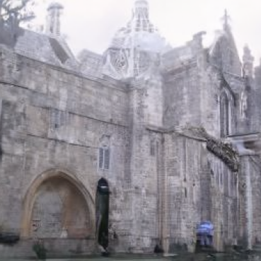
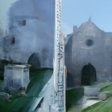
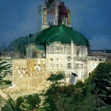
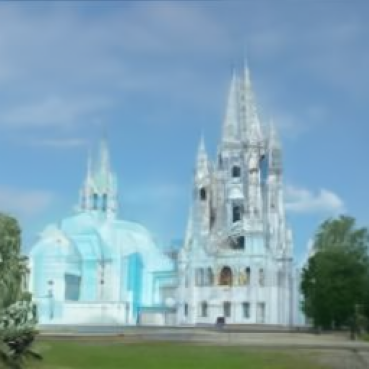
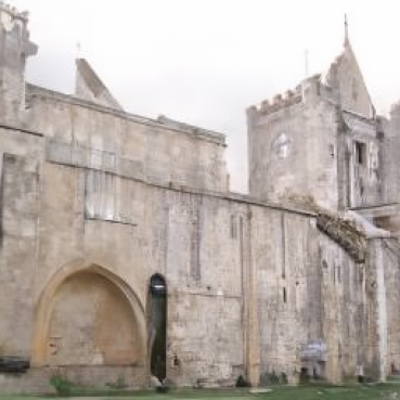
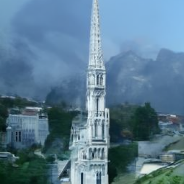
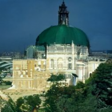
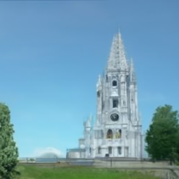
Figure 7: Qualitative results on LSUN-church (Yu et al., 2015) dataset. The first row is unguided samples from DDIM (Song et al., 2021), and the second row is guided samples using our guidance method, DAG.

Qualitative results.

In addition, we compare the result from ADM without our guidance and with our guidance method in Fig. 5. We show both generated images and predicted depth maps using DPT, which demonstrates the effectiveness of our method of generating depth-aware images so that depth prediction models can predict the depth more robustly. Unlike guidance-free sampling, which is shown to generate geometrically implausible results, our method successfully generates depth-aware samples. Moreover, we represent surface normal estimation (Bae et al., 2021) (Fig. 5) and point cloud visualization (Fig. 6) to further show the effectiveness of our method in 3D scene understanding. The predictions made by our method show clearer boundaries and contain a higher level of details in scene geometry, as compared to the baseline. We also provide qualitative comparisons on LSUN-Church between unguided samples and samples using our guidance method in Fig. 7. Similar to the results observed on LSUN-Bedroom, we find that our guidance method can effectively preserve geometric characteristics.

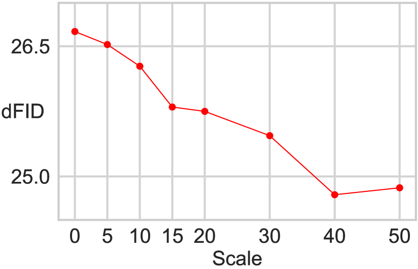
(a) DCG

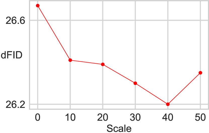
(b) DPG

Figure 8: Comparison of dFID with respect to the guidance scales of DCG and DPG.

5.3 Ablation Study

In this section, we analyze the effectiveness of different experimental settings and choices in our framework. To reduce the effect of random variation, we fix the random seed so that all variants see the same images in the same order. To compute the metrics, we perform all ablation studies on 1K generated samples.

Table 3: Ablation study of the resolution of the depth prior network.

Method	dFID ($\downarrow$)
Baseline	26.77
$32\times 32$	25.14
$64\times 64$	25.96
$128\times 128$	25.07

Table 4: Application for monocular depth estimation. We train the depth estimation model from scratch using U-Net (Ronneberger et al., 2015) based backbone network with our synthesized data.

Method	$\delta>1.25$ ($\uparrow$)	AbsRel. ($\downarrow$)
Supervised	79.06	0.144
Unguided data	72.55	0.185
DAG-based data	77.54	0.151

Guidance scale.

We study the relationship between the guidance scale and image quality in terms of dFID for each DCG and DPG. Fig. 8 shows the tendency of the metrics versus scales of each guidance. As depicted in Fig. 8, DCG and DPG obtains the best results at $\omega_{\mathrm{dc}}=40$ and $\omega_{\mathrm{dp}}=40$ in dFID, respectively. Therefore, we treat this scale as default for the remaining part.

Resolution of the prior network.

In our second guidance method, DPG, we need to train a diffusion network to give a prior for condition image. But there are limitations in computation cost for the sampling process, so we choose the proper model size for the prior diffusion network. As our output depth map has a resolution of $64\times 64$, we interpolate the depth map when fed to the prior network. We test three resolutions: $[32\times 32,64\times 64,128\times 128]$ for the pretrained prior diffusion network, and the quantitative results are shown in Tab. 3. The $128\times 128$ outperforms the other resolution settings.

5.4 Application for Monocular Depth Estimation

To improve the effects of our generation as unlabeled data, we leverage the guided images and corresponding depth maps. We train the U-Net-based depth estimation network (Godard et al., 2019) and evaluate the metrics with the NYU-Depth datasets (Silberman et al., 2012). We compare the training results using reference data, unguided generated results, and our generated results. For the depth evaluation, we use accuracy under the threshold ($\delta<1.25$) and absolute relative error (AbsRel). Tab. 4 shows that the images generated by DAG-based data are more helpful in training the depth predictor than the unguided samples set.

6 Conclusion

In this paper, we propose a label-efficient method for predicting depth maps of images generated by the reverse process of diffusion model using internal representations. We also introduce a novel guidance scheme to guide the image to have a plausible depth map. In addition, to address the problem that existing measurement methods fail to capture the depth feasibility of generated images, we present a new evaluation metric that effectively represents this depth awareness using pretrained depth estimation networks.

Appendix A Further Details

A.1 Implementation Details

Hyperparameter Settings.

We report hyperparameters utilized during the training of the depth estimator and sampling process in Tab. 5. For two datasets, LSUN-Bedroom and LSUN-Church (Yu et al., 2015), the hyperparameters employed for the depth estimator training are largely consistent. Note that we use two different U-Net implementations, namely ADM (Dhariwal & Nichol, 2021) and DDIM (Song et al., 2021), due to the existence of pretrained weights, thus leading to slight variations in the selection of the feature extraction block.

Table 5: Detailed hyperparameter settings. Training denotes hyperparameters used at the training depth estimator, and sampling denotes hyperparameters used at sampling diffusion models using DAG.

	Hyperparameters	LSUN-Bedroom (Yu et al., 2015)	LSUN-Church (Yu et al., 2015)
Training	learning rate	$1e-5$	$1e-5$
	optimizer	Adam	Adam
	$\mathbf{g}^{W}$	$[\mathbf{f}_{t}(6)]$	$[\mathbf{f}_{t}(17)]$
	$\mathbf{g}^{S}$	$[\mathbf{f}_{t}(2);\mathbf{f}_{t}(4);\mathbf{f}_{t}(5);\mathbf{f}_{t}(6);\mathbf{f}_{t}(7)]$	$[\mathbf{f}_{t}(3);\mathbf{f}_{t}(5);\mathbf{f}_{t}(7);\mathbf{f}_{t}(9);\mathbf{f}_{t}(13);\mathbf{f}_{t}(17)]$
	Timestep Sampler	Uniform	Uniform
	Time embedding dimension	256	256
Sampling	Timestep	25	25
	Schedular	DDIM	DDIM
	$\tau$	Uniform	Uniform
	$\omega_{dc}$	40.0	10.0
	$\omega_{dp}$	40.0	50.0

A.2 PyTorch-like Pseudo Code.

Guidance Method.

We provide a detailed PyTorch-like pseudo-code of our guidance method in Algorithm 1.

Network Architecture for Depth Estimator.

We use a 3-layer MLP that receives concatenated feature vector of a pixel to predict the depth map. Following the diffusion network, we apply the SiLU activation function. Detailed architecture is shown in Fig. 2 of the main paper and Algorithm 2 of this appendix. Also, we add a time-embedding module to this depth estimator MLP following the implementation of U-Net of ADM (Dhariwal & Nichol, 2021).

Algorithm 1 Pseudo Code of Our Depth-Aware Guidance

⬇

def cond_fn(img, t, y=None):

"""

␣␣␣␣dc:␣scale␣of␣depth␣consistency␣guidance

␣␣␣␣dp:␣scale␣of␣depth␣prior␣guidance

␣␣␣␣"""

img = img.detach().requires_grad_(True)

# feature extraction

strong_feature, weak_feature = feature_extractor(img, t)

# depth consistency loss

strong_depth = strong_depth_predictor(strong_feature, t)

weak_depth = weak_depth_predictor(weak_feature, t)

dcg_loss = F.l1_loss(weak_depth, strong_depth.detach())

# depth prior loss

noise = torch.randn_like(strong_depth)

t_rand = torch.randint(0, 25)

strong_depth_t = diffusion.q_sample(strong_depth, t_rand, noise=noise)

strong_eps = prior_diffusion_model(strong_depth_t, t_rand)

dpg_loss = torch.mean((strong_eps - noise) ** 2)

loss = dp * dpg_loss + dc * dcg_loss

grad = torch.autograd.grad(loss, img, allow_unused=True)[0]

return -1.0 * grad

Algorithm 2 Pseudo Code of Our Label-efficient Depth Estimator

⬇

class MLPBlock(nn.Module):

def __init__(self, in_dim, out_dim, time_dim):

super().__init__()

self.linear = nn.Linear(in_dim, out_dim)

self.is_last = True if out_dim == 1 else False

if not self.is_last:

self.act = nn.SiLU()

self.norm = nn.BatchNorm1d(out_dim)

self.time_proj = nn.Linear(time_dim, out_dim)

else:

self.act = nn.Sigmoid()

self.norm = nn.Identity()

self.time_proj = None

def forward(self, x, time_emb=None):

x = self.linear(x)

x = self.act(x)

x = self.norm(x)

if not self.is_last:

x = x + self.time_proj(time_emb)

return x

⬇

class DepthPredictor(nn.Module):

def __init__(self, dim):

super().__init__()

self.layers = nn.ModuleList([

MLPBlock(dim, 256, time_dim=256),

MLPBlock(256, 128, time_dim=256),

MLPBlock(128, 1, time_dim=256),

])

self.max_depth = 10.0

def forward(self, x, timesteps=None):

timesteps = timestep_embedding(timesteps, 256)

for layer in self.layers:

x = layer(x, timesteps)

return x * self.max_depth

A.3 Proposed Metric

Table 6: Comparison of generated samples from ADM. The images in the left two columns are examples of samples from ADM without our guidance method, DAG, and the images in the right two columns are examples from ADM using our method.

Samples
DAG	✗		✓
dFID ($\downarrow$)	15.71		13.93
FID ($\downarrow$)	6.72		7.59

We propose a new metric, called dFID, which can evaluate the depth-awareness, and we describe the details of the proposed metrics in this section.

Depth FID.

To compute the FID of the depth domain, we first estimate the depth map using the NYU-Depth (Silberman et al., 2012) pretrained depth estimator DPT-Hybrid (Ranftl et al., 2021), which is available in the official repository. Then, identical to the original FID, we compute the Fréchet distance of embeddings collected from depth images using the Inception v3 model (Szegedy et al., 2015). We show examples in Tab. 6 where FID is good but the geometric realism is limited. It demonstrates that the FID is inappropriate for measuring geometrical awareness. To address this problem, we propose dFID. DAG, our proposed guidance method, improves both the visual quality of geometric realism and the dFID metric. However, in terms of FID, we can find that FID does not adequately capture the geometric plausibility.

Appendix B More Visualizations

Furthermore, we show additional qualitative results in Fig. 9 comparing the performance of the baseline and our proposed guidance approach. The images generated using our guidance approach exhibit reduced perspective ambiguity and a more accurate portrayal of the layout when compared to the baseline. Additionally, through visualizations of the related depth maps, it is evident that the diffusion models guided by our approach produce more geometrically plausible outcomes than those generated without guidance.

B.1 Point Cloud Visualization

We provide supplementary results in Fig. 10 that demonstrate the point cloud derived from the images, as well as its related depth, to highlight the depth awareness and geometric plausibility of our proposed guidance approach. To provide a comprehensive evaluation, we have generated point clouds from multiple perspectives, such as front, left, right, and upward, using the Open3D library (Zhou et al., 2018), in order to compare the 3D-represented images. The point cloud representations of the guided samples are observed to be more consistent and realistic when viewed from the same perspective, and they exhibit robust geometric consistency.

B.2 Surface Normal Visualization

Fig. 11 also presents the results of surface normal estimation for both the baseline method and our proposed methodology. We employ surface normals to evaluate the geometrical rationality of the generated images as they are a crucial feature of geometric surfaces. Furthermore, by computing the probability distribution of the per-pixel surface normal, we estimate the aleatoric uncertainty (Bae et al., 2021). It can be observed that when compared to the baseline, our method’s predictions exhibit a more defined layout and bounds, resulting in lower uncertainty along the borders of walls.

Appendix C Limitations and Future Works

In this study, we focus on the sampling strategy that leads to the generation of images with higher depth awareness. This strategy enables the use of generated images with more reliable and precise geometric properties in a variety of downstream tasks. As our work represents the first attempt to enable depth awareness in image synthesis using diffusion models, it is challenging to compare its performance to previous research. we have employed pretrained diffusion models in this study due to the high computational cost of the training, and the data selection was also limited. In future research, we plan to train the diffusion model using indoor and outdoor scene datasets to directly demonstrate and improve the effectiveness of our guiding technique. Additionally, while we have employed the diffusion U-Net as part of the depth estimator, this approach increases the cost of the guiding process through the gradient computation demands of backpropagation through the whole U-Net. An alternative approach to address this challenge would be to train the diffusion network using depth map conditioning and sampling with classifier-free guidance, however, this would require a significant amount of depth-image pairs and computational resources for joint training, compared to our current method.

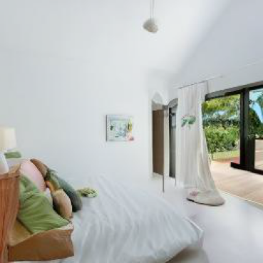
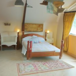
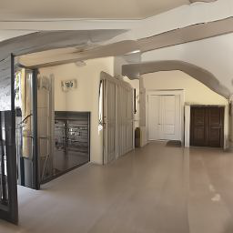
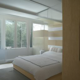
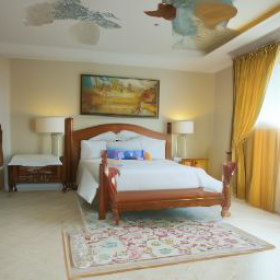
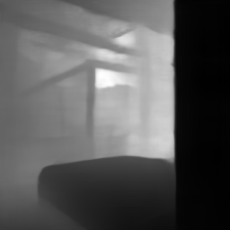
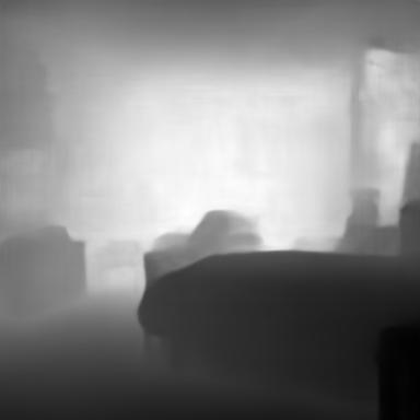
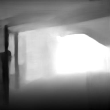
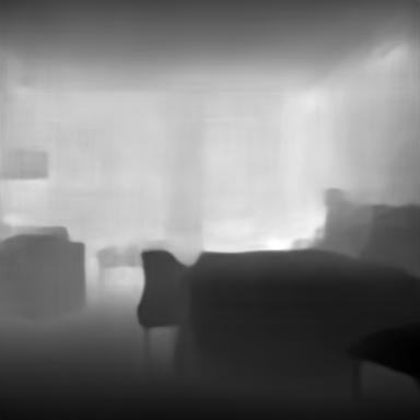
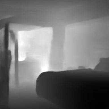
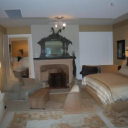
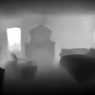
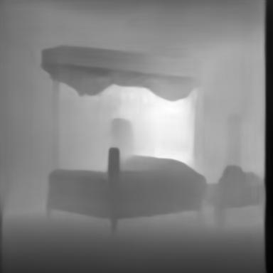
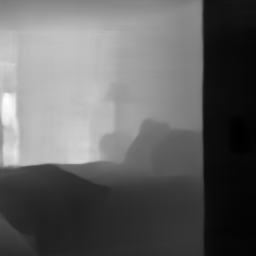
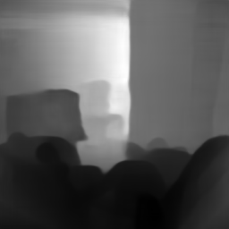
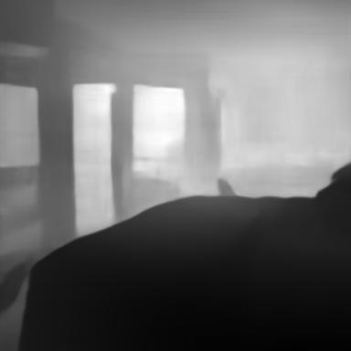
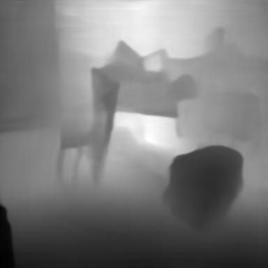
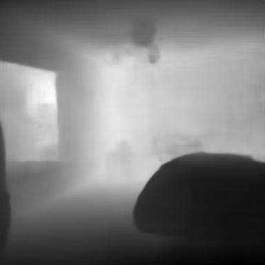
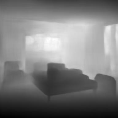
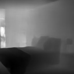
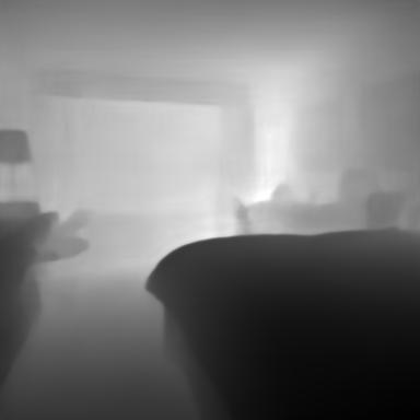
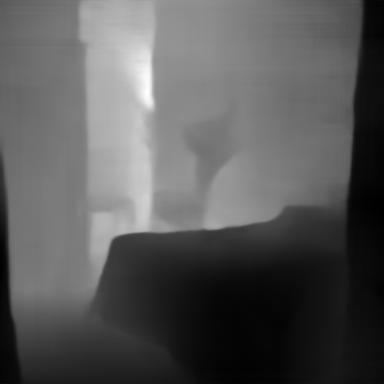
Figure 9: Qualitative comparison on LSUN bedroom datasets (Yu et al., 2015). We show the results of unguided and depth-guided samples (first two rows) and their corresponding depths (last two rows).

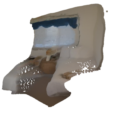
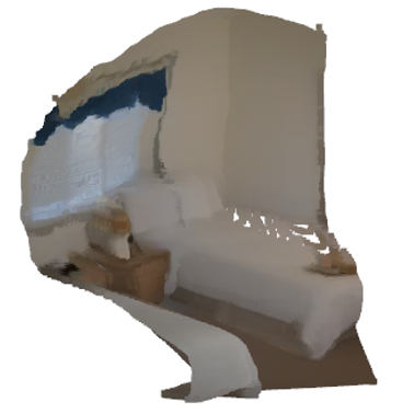
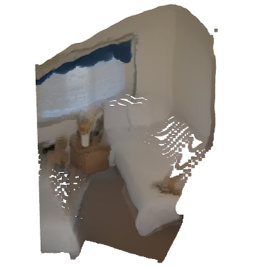
(a)
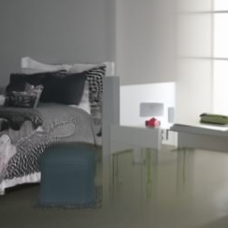
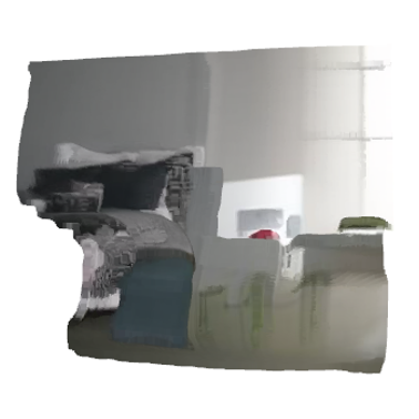
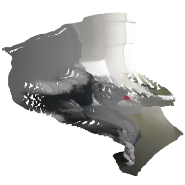
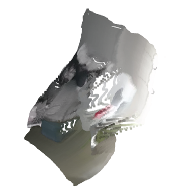
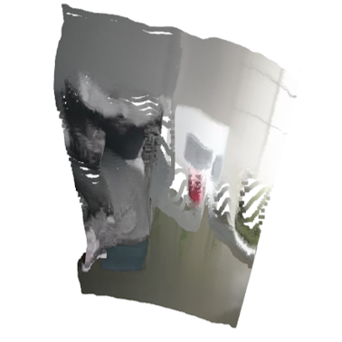
(b)
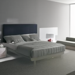
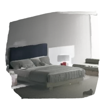
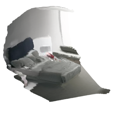
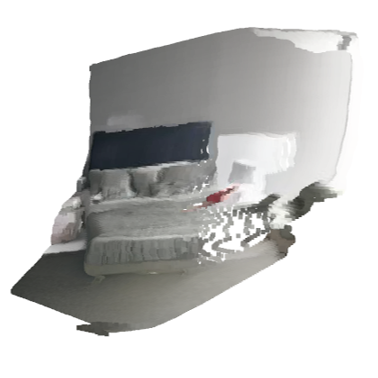
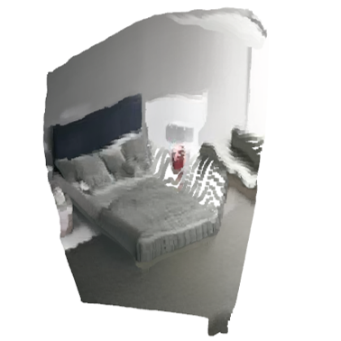
(c)
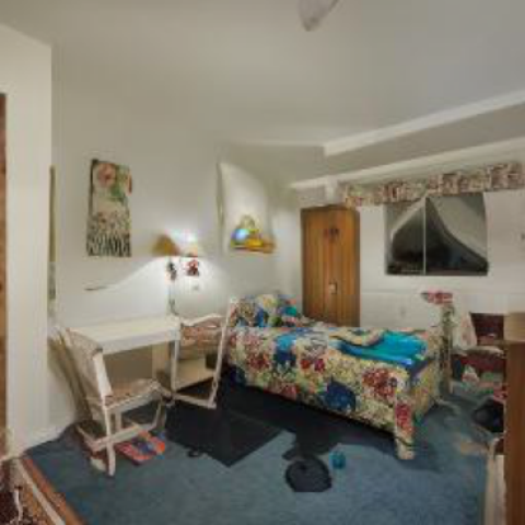
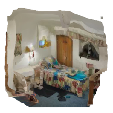
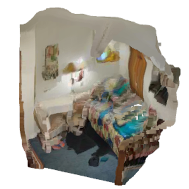
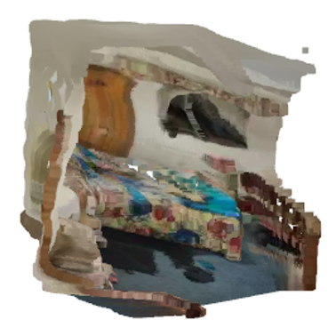
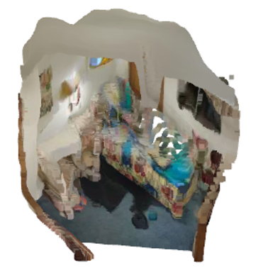
(d)
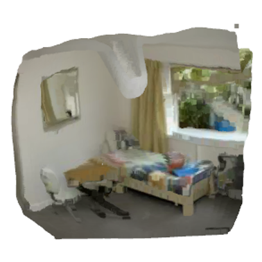
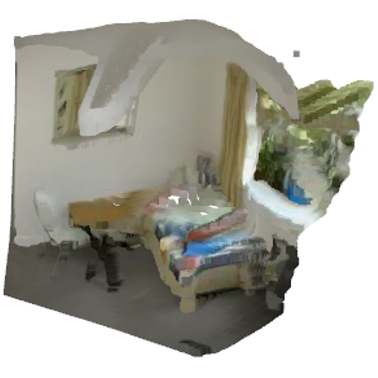
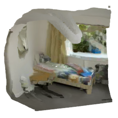
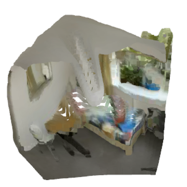
(e)
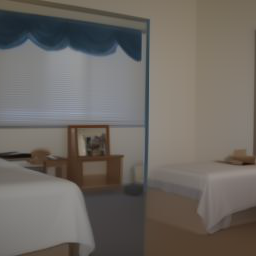
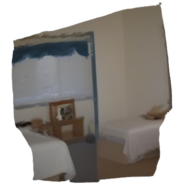
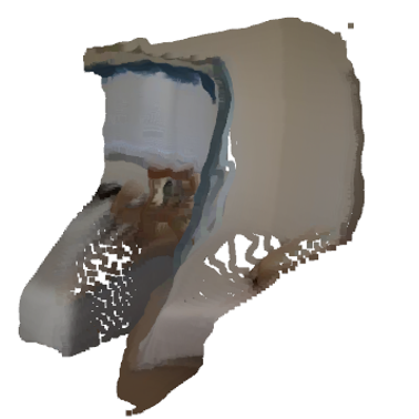
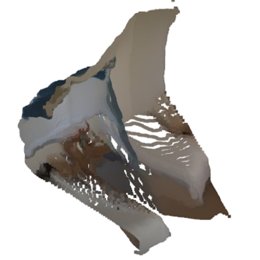
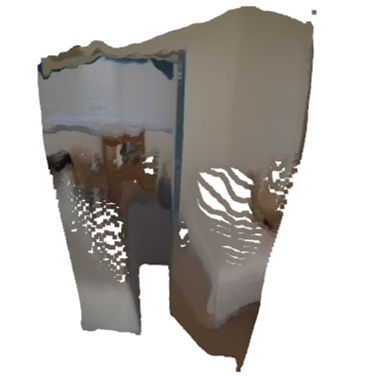
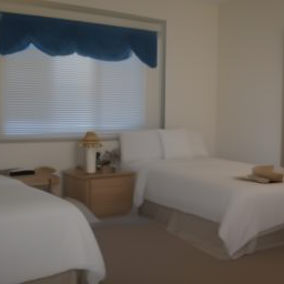
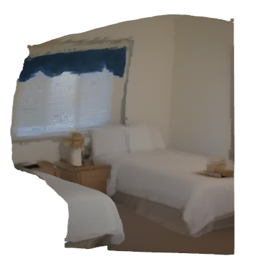
(f)	(a) synthesized image	(b) front (c) right (d) left (e) up

Figure 10: Visualization of point cloud representation obtained by depth information. (a), (c), (e) are generated samples from ADM, and (b), (d), (f) are samples from ADM with our guidance method. The left column is generated image, and the other columns are point cloud visualizations from four different views.

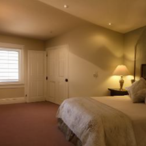
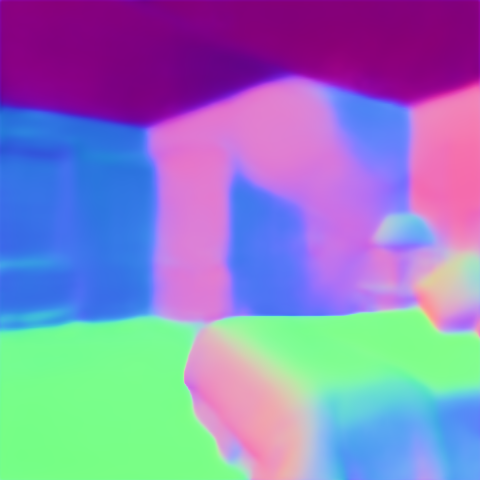
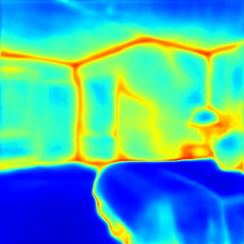
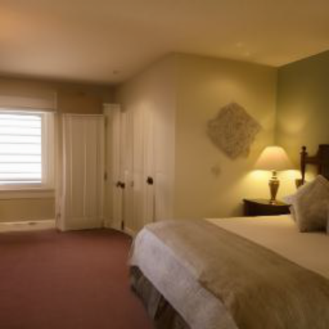
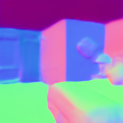
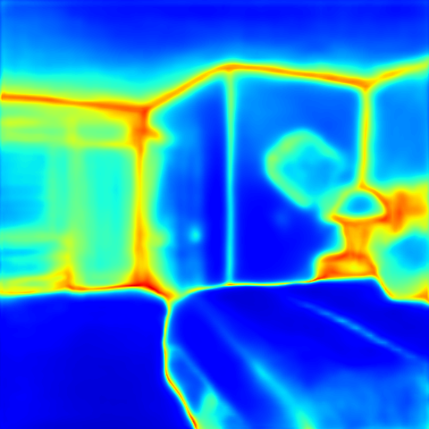
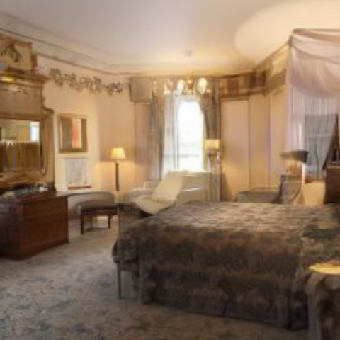
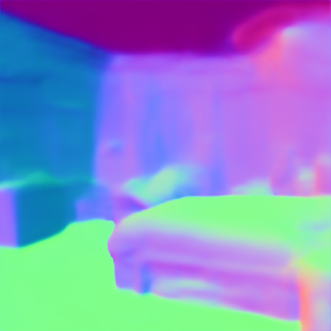
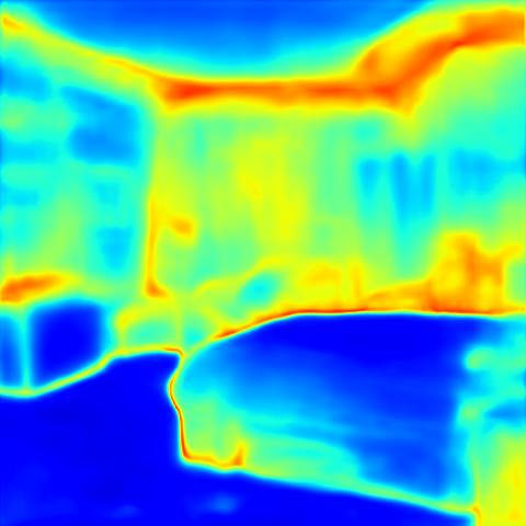
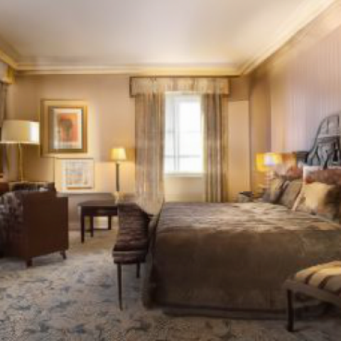
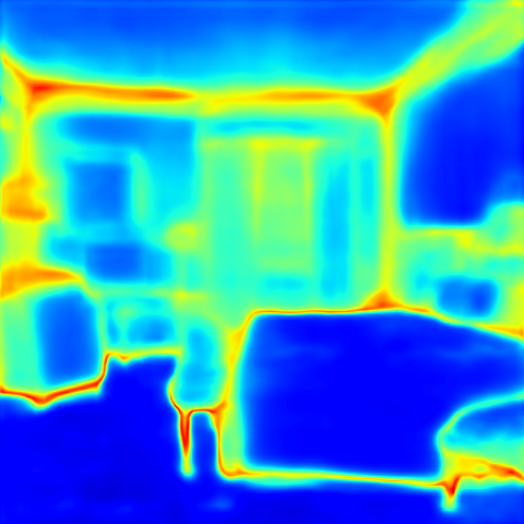
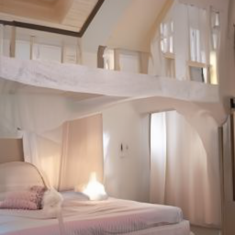
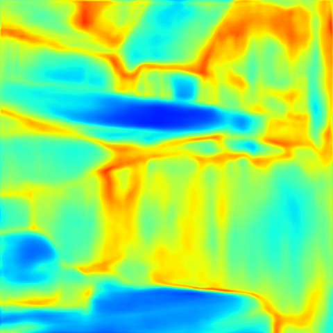
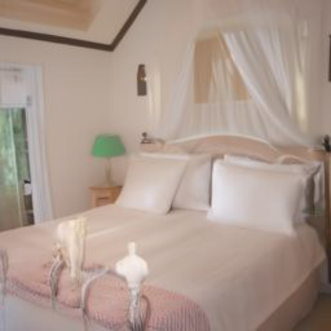
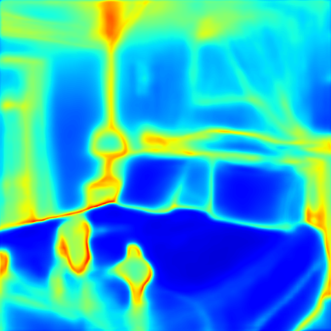
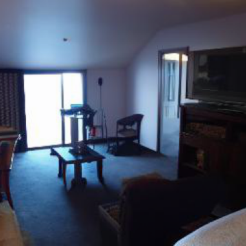
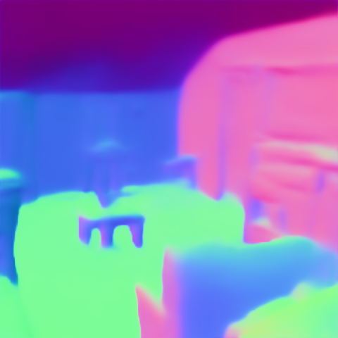
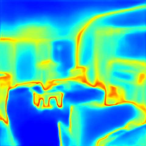
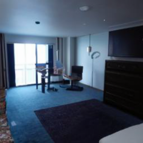
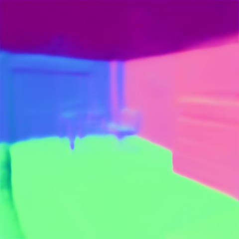
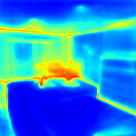
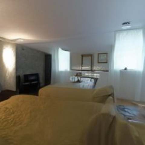
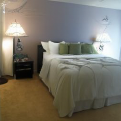
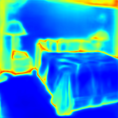
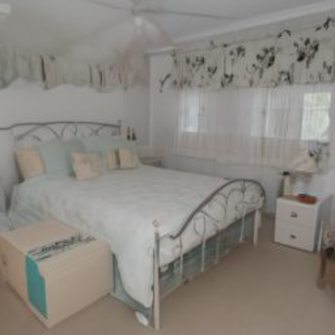
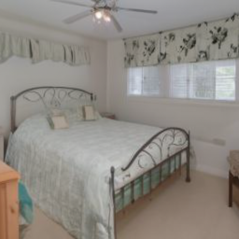
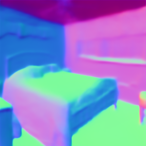
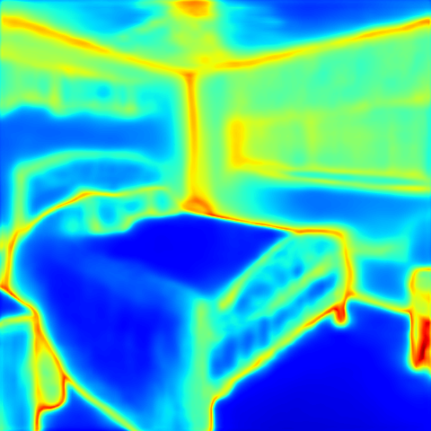
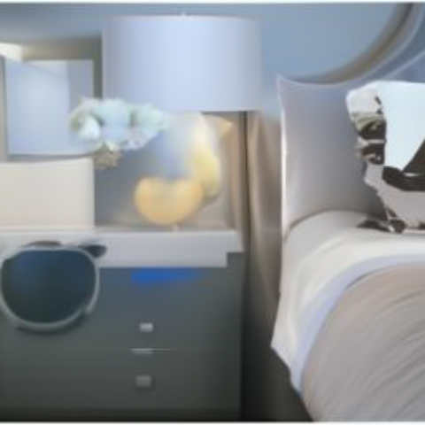
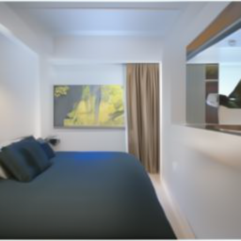
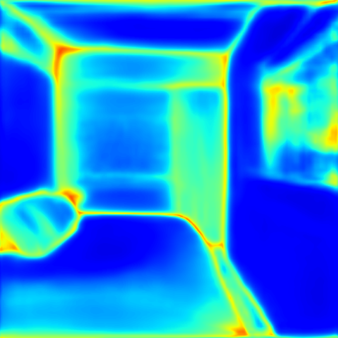
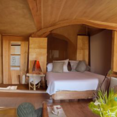
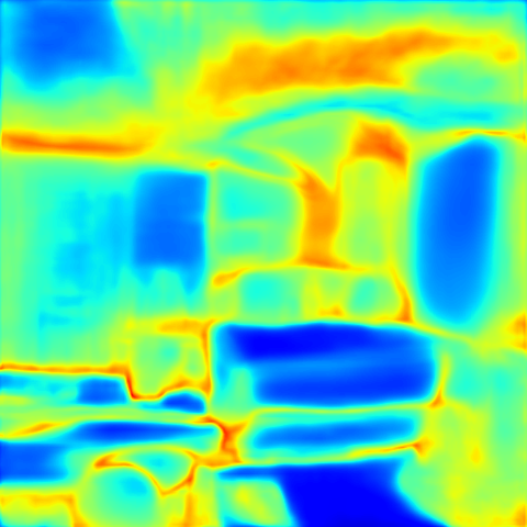
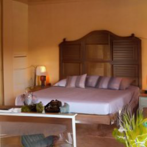
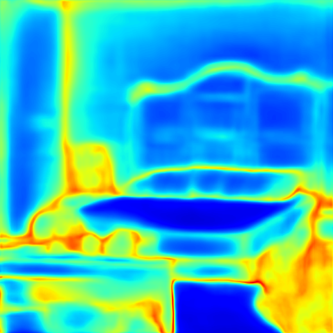
Figure 11: Qualitative comparison of the baseline and our method using surface normals and corresponding uncertainty.

References

- Asiedu et al. (2022) Asiedu, E. B., Kornblith, S., Chen, T., Parmar, N., Minderer, M., and Norouzi, M. Decoder denoising pretraining for semantic segmentation. arXiv preprint arXiv: Arxiv-2205.11423, 2022.
- Bachman et al. (2014) Bachman, P., Alsharif, O., and Precup, D. Learning with pseudo-ensembles. Advances in neural information processing systems, 27, 2014.
- Bae et al. (2021) Bae, G., Budvytis, I., and Cipolla, R. Estimating and exploiting the aleatoric uncertainty in surface normal estimation. In Proceedings of the IEEE/CVF International Conference on Computer Vision (ICCV), pp. 13137–13146, October 2021.
- Balaji et al. (2022) Balaji, Y., Nah, S., Huang, X., Vahdat, A., Song, J., Kreis, K., Aittala, M., Aila, T., Laine, S., Catanzaro, B., et al. ediffi: Text-to-image diffusion models with an ensemble of expert denoisers. arXiv preprint arXiv:2211.01324, 2022.
- Baranchuk et al. (2022) Baranchuk, D., Voynov, A., Rubachev, I., Khrulkov, V., and Babenko, A. Label-efficient semantic segmentation with diffusion models. In International Conference on Learning Representations, 2022. URL https://openreview.net/forum?id=SlxSY2UZQT.
- Bhat et al. (2021) Bhat, S. F., Alhashim, I., and Wonka, P. Adabins: Depth estimation using adaptive bins. In CVPR, pp. 4009–4018, 2021.
- Chen & He (2021) Chen, X. and He, K. Exploring simple siamese representation learning. In Proceedings of the IEEE/CVF Conference on Computer Vision and Pattern Recognition, pp. 15750–15758, 2021.
- Choi et al. (2021) Choi, J., Kim, S., Jeong, Y., Gwon, Y., and Yoon, S. Ilvr: Conditioning method for denoising diffusion probabilistic models. arXiv preprint arXiv:2108.02938, 2021.
- Dhariwal & Nichol (2021) Dhariwal, P. and Nichol, A. Diffusion models beat gans on image synthesis. Advances in Neural Information Processing Systems, 34:8780–8794, 2021.
- Dosovitskiy et al. (2020) Dosovitskiy, A., Beyer, L., Kolesnikov, A., Weissenborn, D., Zhai, X., Unterthiner, T., Dehghani, M., Minderer, M., Heigold, G., Gelly, S., et al. An image is worth 16x16 words: Transformers for image recognition at scale. arXiv preprint arXiv:2010.11929, 2020.
- Eigen et al. (2014) Eigen, D., Puhrsch, C., and Fergus, R. Depth map prediction from a single image using a multi-scale deep network. Advances in neural information processing systems, 27, 2014.
- Esser et al. (2020) Esser, P., Rombach, R., and Ommer, B. Taming transformers for high-resolution image synthesis, 2020.
- Farid (2022) Farid, H. Perspective (in) consistency of paint by text. arXiv preprint arXiv:2206.14617, 2022.
- Fu et al. (2018) Fu, H., Gong, M., Wang, C., Batmanghelich, K., and Tao, D. Deep ordinal regression network for monocular depth estimation. In CVPR, pp. 2002–2011, 2018.
- Godard et al. (2019) Godard, C., Mac Aodha, O., Firman, M., and Brostow, G. J. Digging into self-supervised monocular depth estimation. In Proceedings of the IEEE/CVF International Conference on Computer Vision, pp. 3828–3838, 2019.
- Goodfellow et al. (2014) Goodfellow, I., Pouget-Abadie, J., Mirza, M., Xu, B., Warde-Farley, D., Ozair, S., Courville, A., and Bengio, Y. Generative adversarial nets. Advances in neural information processing systems, 27, 2014.
- Goodfellow et al. (2020) Goodfellow, I., Pouget-Abadie, J., Mirza, M., Xu, B., Warde-Farley, D., Ozair, S., Courville, A., and Bengio, Y. Generative adversarial networks. Communications of the ACM, 63(11):139–144, 2020.
- Graikos et al. (2022) Graikos, A., Malkin, N., Jojic, N., and Samaras, D. Diffusion models as plug-and-play priors. arXiv preprint arXiv:2206.09012, 2022.
- Gu et al. (2022) Gu, S., Chen, D., Bao, J., Wen, F., Zhang, B., Chen, D., Yuan, L., and Guo, B. Vector quantized diffusion model for text-to-image synthesis. In Proceedings of the IEEE/CVF Conference on Computer Vision and Pattern Recognition, pp. 10696–10706, 2022.
- Ho & Salimans (2021) Ho, J. and Salimans, T. Classifier-free diffusion guidance. In NeurIPS 2021 Workshop on Deep Generative Models and Downstream Applications, 2021.
- Ho et al. (2020) Ho, J., Jain, A., and Abbeel, P. Denoising diffusion probabilistic models. Advances in Neural Information Processing Systems, 33:6840–6851, 2020.
- Hong et al. (2022) Hong, S., Lee, G., Jang, W., and Kim, S. Improving sample quality of diffusion models using self-attention guidance. arXiv preprint arXiv:2210.00939, 2022.
- Kawar et al. (2022) Kawar, B., Elad, M., Ermon, S., and Song, J. Denoising diffusion restoration models. arXiv preprint arXiv:2201.11793, 2022.
- Kim et al. (2016) Kim, S., Park, K., Sohn, K., and Lin, S. Unified depth prediction and intrinsic image decomposition from a single image via joint convolutional neural fields. In ECCV, pp. 143–159, 2016.
- Kingma & Ba (2014) Kingma, D. P. and Ba, J. Adam: A method for stochastic optimization. arXiv preprint arXiv:1412.6980, 2014.
- Laina et al. (2016) Laina, I., Rupprecht, C., Belagiannis, V., Tombari, F., and Navab, N. Deeper depth prediction with fully convolutional residual networks. In 3DV, pp. 239–248. IEEE, 2016.
- Laine & Aila (2016) Laine, S. and Aila, T. Temporal ensembling for semi-supervised learning. arXiv preprint arXiv:1610.02242, 2016.
- Lee et al. (2013) Lee, D.-H. et al. Pseudo-label: The simple and efficient semi-supervised learning method for deep neural networks. In Workshop on challenges in representation learning, ICML, volume 3, pp. 896, 2013.
- Lee et al. (2019) Lee, J. H., Han, M.-K., Ko, D. W., and Suh, I. H. From big to small: Multi-scale local planar guidance for monocular depth estimation. arXiv, 2019.
- Li et al. (2015) Li, B., Shen, C., Dai, Y., Van Den Hengel, A., and He, M. Depth and surface normal estimation from monocular images using regression on deep features and hierarchical crfs. In Proceedings of the IEEE conference on computer vision and pattern recognition, pp. 1119–1127, 2015.
- Li et al. (2022) Li, Z., Chen, Z., Liu, X., and Jiang, J. Depthformer: Exploiting long-range correlation and local information for accurate monocular depth estimation. arXiv preprint arXiv:2203.14211, 2022.
- Lin et al. (2022) Lin, C.-H., Gao, J., Tang, L., Takikawa, T., Zeng, X., Huang, X., Kreis, K., Fidler, S., Liu, M.-Y., and Lin, T.-Y. Magic3d: High-resolution text-to-3d content creation. arXiv preprint arXiv:2211.10440, 2022.
- Lin et al. (2013) Lin, D., Fidler, S., and Urtasun, R. Holistic scene understanding for 3d object detection with rgbd cameras. In Proceedings of the IEEE international conference on computer vision, pp. 1417–1424, 2013.
- Meng et al. (2021) Meng, C., He, Y., Song, Y., Song, J., Wu, J., Zhu, J.-Y., and Ermon, S. Sdedit: Guided image synthesis and editing with stochastic differential equations. In International Conference on Learning Representations, 2021.
- Nathan Silberman & Fergus (2012) Nathan Silberman, Derek Hoiem, P. K. and Fergus, R. Indoor segmentation and support inference from rgbd images. In ECCV, 2012.
- Nichol et al. (2021) Nichol, A., Dhariwal, P., Ramesh, A., Shyam, P., Mishkin, P., McGrew, B., Sutskever, I., and Chen, M. Glide: Towards photorealistic image generation and editing with text-guided diffusion models. arXiv preprint arXiv:2112.10741, 2021.
- Nichol & Dhariwal (2021) Nichol, A. Q. and Dhariwal, P. Improved denoising diffusion probabilistic models. In International Conference on Machine Learning, pp. 8162–8171. PMLR, 2021.
- Poole et al. (2022) Poole, B., Jain, A., Barron, J. T., and Mildenhall, B. Dreamfusion: Text-to-3d using 2d diffusion. arXiv preprint arXiv:2209.14988, 2022.
- Ramesh et al. (2022) Ramesh, A., Dhariwal, P., Nichol, A., Chu, C., and Chen, M. Hierarchical text-conditional image generation with clip latents. arXiv preprint arXiv:2204.06125, 2022.
- Ranftl et al. (2021) Ranftl, R., Bochkovskiy, A., and Koltun, V. Vision transformers for dense prediction. In Proceedings of the IEEE/CVF International Conference on Computer Vision, pp. 12179–12188, 2021.
- Rombach et al. (2022) Rombach, R., Blattmann, A., Lorenz, D., Esser, P., and Ommer, B. High-resolution image synthesis with latent diffusion models. In Proceedings of the IEEE/CVF Conference on Computer Vision and Pattern Recognition, pp. 10684–10695, 2022.
- Ronneberger et al. (2015) Ronneberger, O., Fischer, P., and Brox, T. U-net: Convolutional networks for biomedical image segmentation. In International Conference on Medical image computing and computer-assisted intervention, pp. 234–241. Springer, 2015.
- Saharia et al. (2022a) Saharia, C., Chan, W., Chang, H., Lee, C., Ho, J., Salimans, T., Fleet, D., and Norouzi, M. Palette: Image-to-image diffusion models. In ACM SIGGRAPH 2022 Conference Proceedings, pp. 1–10, 2022a.
- Saharia et al. (2022b) Saharia, C., Chan, W., Saxena, S., Li, L., Whang, J., Denton, E., Ghasemipour, S. K. S., Ayan, B. K., Mahdavi, S. S., Lopes, R. G., et al. Photorealistic text-to-image diffusion models with deep language understanding. arXiv preprint arXiv:2205.11487, 2022b.
- Saharia et al. (2022c) Saharia, C., Ho, J., Chan, W., Salimans, T., Fleet, D. J., and Norouzi, M. Image super-resolution via iterative refinement. IEEE Transactions on Pattern Analysis and Machine Intelligence, 2022c.
- Sajjadi et al. (2016) Sajjadi, M., Javanmardi, M., and Tasdizen, T. Regularization with stochastic transformations and perturbations for deep semi-supervised learning. Advances in neural information processing systems, 29, 2016.
- Seo et al. (2022) Seo, J., Lee, G., Cho, S., Lee, J., and Kim, S. Midms: Matching interleaved diffusion models for exemplar-based image translation. arXiv preprint arXiv:2209.11047, 2022.
- Shi et al. (2022) Shi, Z., Shen, Y., Zhu, J., Yeung, D.-Y., and Chen, Q. 3d-aware indoor scene synthesis with depth priors. arXiv preprint arXiv:2202.08553, 2022.
- Silberman et al. (2012) Silberman, N., Hoiem, D., Kohli, P., and Fergus, R. Indoor segmentation and support inference from rgbd images. In European conference on computer vision, pp. 746–760. Springer, 2012.
- Sohl-Dickstein et al. (2015) Sohl-Dickstein, J., Weiss, E., Maheswaranathan, N., and Ganguli, S. Deep unsupervised learning using nonequilibrium thermodynamics. In International Conference on Machine Learning, pp. 2256–2265. PMLR, 2015.
- Sohn et al. (2020) Sohn, K., Berthelot, D., Carlini, N., Zhang, Z., Zhang, H., Raffel, C. A., Cubuk, E. D., Kurakin, A., and Li, C.-L. Fixmatch: Simplifying semi-supervised learning with consistency and confidence. NIPS, 33:596–608, 2020.
- Song et al. (2021) Song, J., Meng, C., and Ermon, S. Denoising diffusion implicit models. In International Conference on Learning Representations, 2021. URL https://openreview.net/forum?id=St1giarCHLP.
- Song et al. (2020) Song, Y., Sohl-Dickstein, J., Kingma, D. P., Kumar, A., Ermon, S., and Poole, B. Score-based generative modeling through stochastic differential equations. arXiv preprint arXiv:2011.13456, 2020.
- Szegedy et al. (2015) Szegedy, C., Vanhoucke, V., Ioffe, S., Shlens, J., and Wojna, Z. Rethinking the inception architecture for computer vision. arXiv preprint arXiv: Arxiv-1512.00567, 2015.
- Tateno et al. (2017) Tateno, K., Tombari, F., Laina, I., and Navab, N. Cnn-slam: Real-time dense monocular slam with learned depth prediction. In Proceedings of the IEEE conference on computer vision and pattern recognition, pp. 6243–6252, 2017.
- Tewari et al. (2022) Tewari, A., Pan, X., Fried, O., Agrawala, M., Theobalt, C., et al. Disentangled3d: Learning a 3d generative model with disentangled geometry and appearance from monocular images. In Proceedings of the IEEE/CVF Conference on Computer Vision and Pattern Recognition, pp. 1516–1525, 2022.
- Ummenhofer et al. (2017) Ummenhofer, B., Zhou, H., Uhrig, J., Mayer, N., Ilg, E., Dosovitskiy, A., and Brox, T. Demon: Depth and motion network for learning monocular stereo. In CVPR, pp. 5038–5047, 2017.
- Vaswani et al. (2017) Vaswani, A., Shazeer, N., Parmar, N., Uszkoreit, J., Jones, L., Gomez, A. N., Kaiser, Ł., and Polosukhin, I. Attention is all you need. NIPS, 30, 2017.
- Vincent et al. (2008) Vincent, P., Larochelle, H., Bengio, Y., and Manzagol, P.-A. Extracting and composing robust features with denoising autoencoders. In Proceedings of the 25th International Conference on Machine learning, pp. 1096–1103, 2008.
- von Platen et al. (2022) von Platen, P., Patil, S., Lozhkov, A., Cuenca, P., Lambert, N., Rasul, K., Davaadorj, M., and Wolf, T. Diffusers: State-of-the-art diffusion models. https://github.com/huggingface/diffusers, 2022.
- Wang et al. (2022a) Wang, T., Zhang, T., Zhang, B., Ouyang, H., Chen, D., Chen, Q., and Wen, F. Pretraining is all you need for image-to-image translation. arXiv preprint arXiv:2205.12952, 2022a.
- Wang et al. (2022b) Wang, W., Bao, J., Zhou, W., Chen, D., Chen, D., Yuan, L., and Li, H. Semantic image synthesis via diffusion models. arXiv preprint arXiv:2207.00050, 2022b.
- Wang et al. (2015) Wang, X., Fouhey, D., and Gupta, A. Designing deep networks for surface normal estimation. In CVPR, pp. 539–547, 2015.
- Wang et al. (2019) Wang, Y., Chao, W.-L., Garg, D., Hariharan, B., Campbell, M., and Weinberger, K. Q. Pseudo-lidar from visual depth estimation: Bridging the gap in 3d object detection for autonomous driving. In Proceedings of the IEEE/CVF Conference on Computer Vision and Pattern Recognition, pp. 8445–8453, 2019.
- Yu et al. (2015) Yu, F., Seff, A., Zhang, Y., Song, S., Funkhouser, T., and Xiao, J. Lsun: Construction of a large-scale image dataset using deep learning with humans in the loop. arXiv preprint arXiv:1506.03365, 2015.
- Zhou et al. (2018) Zhou, Q.-Y., Park, J., and Koltun, V. Open3D: A modern library for 3D data processing. arXiv:1801.09847, 2018.