Comparing Voting Districts with Uncertain Data Envelopment Analysis

Abstract

Gerrymandering voting districts is one of the most salient concerns of contemporary American society, and the creation of new voting maps, along with their subsequent legal challenges, speaks for much of our modern political discourse. The legal, societal, and political debate over serviceable voting districts demands a concept of fairness, which is a loosely characterized, but amorphous, concept that has evaded precise definition. We advance a new paradigm to compare voting maps that avoids the pitfalls associated with an a priori metric being used to uniformly assess maps. Our evaluative method instead shows how to use uncertain data envelopment analysis to assess maps on a variety of metrics, a tactic that permits each district to be assessed separately and optimally. We test our methodology on a collection of proposed and publicly available maps to illustrate our assessment strategy.

Keywords: Data Envelopment Analysis, Robust Optimization,
                 Gerrymandering

1 Introduction and Strategy

The question of how to draw congressional boundaries in the US is among the most politically charged of debates, and as such, it has drawn significant attention in both our contemporary literature, see e.g. [2, 8, 19, 22], and in our academic literature, see [3, 4, 6, 15, 16, 17, 18, 20, 23] as well as the related districting problems in [5, 9, 12]. Recent concerns about partisan tactics have lead to legal cases [24], and gerrymandering has been linked to economic impacts [1]. Moreover, there are numerous amalgamations of federal and state laws that blur any sense of an ideal process, a fact that regularly promotes wrangling among political factions.

Our goal here is not to enter the highly contested fray of drawing congressional boundaries per se, and we are not advocating for any specific type of map or for any particular map quality. We instead have the singular goal to demonstrate that it is reasonable to compare different congressional maps relative to a collection of agreed upon characteristics. We example a couple of justifiable characteristics and use them to compute a map’s proximity to equitable efficiency [11], which is an evaluation that permits each map, and indeed each district, to be assessed on its own optimal metric. The map closest to equitable efficiency is then declared to be the best of the comparative cohort.

We adopt the sense of efficiency from data envelopment analysis (DEA), which is a stalwart analytic technique that separates decision making units (DMUs) into those that are efficient and those that are not. There are numerous DEA adaptations, see [7] as a review, but we build from the recent work in [10, 11], the latter of which defines the proximity to equitable efficiency. We neither review DEA nor its recent robust/uncertain extensions for the sake of brevity, although readers can find recent reviews and advances in [21, 25, 26]. The proximity to equitable efficiency is the smallest amount of uncertainty required of the defining characteristics so that all DMUs have a claim to efficiency with an appropriate selection of data from within the collection of uncertain possibilities. So a collection of DMUs with a small proximity value indicates a shared efficiency status, whereas a large proximity value suggests disparities among the DMUs. We note that small proximity values do not imply similar characteristics but instead mean that each DMU has a way to weight its defining characteristics to reach an efficiency score of one.

1.1 Characteristic Data

Congressional districts segment a state’s population by assigning individuals to districts, and we assume that $C^{s}$ represents a district and that $\mathcal{C}=\{C^{s}:s=1,2,\ldots,S\}$ is a proposed map for a particular state. We select two characteristics for each district, one input and one output, the intents of which are:

input-characteristic —

minimize wasted votes, and

output-characteristic —

maximize proportional representation.

We tout the use of one input and one output in our example because the proximity value is restricted within a range whose bounds have a ratio no greater than $\sqrt{2}$, which is the smallest possible ratio [14]. The use of only two characteristics further supports graphical interpretation. However, our assessment strategy extends to an arbitrary number of inputs and outputs, and political and social scientists could straightforwardly include more and different characteristics.

Eight different maps are compared for each state from FiveThiryEight’s The Atlas of Redistricting. Each district in the atlas associates with 1) a chance of being represented by a democrat, 2) a chance of being represented by a republican, and 3) the size of the voting age population, as well as several other statistics. We further collect the political leaning of each state from the Pew Research Center, data that divides each state’s population into percentages that are, or lean, republican; are, or lean, democrat; and that have no tendency. We simplify this information by evenly splitting the percentage having no tendency between the other two categories. We use the following notation for these statistics:

$\rho^{D}_{skt}$	–	chance that district $s$ in state $k$
		under map $t$ goes democratic,
$\rho^{R}_{skt}$	–	chance that district $s$ in state $k$
		under map $t$ goes republican,
$v_{skt}$	–	voting age population of district $s$
		in state $k$ under map $t$,
$\ell^{D}_{k}$	–	likely percentage to vote democratic
		in state $k$, and
$\ell^{R}_{k}$	–	likely percentage to vote republican
		in state $k$.

We assume two parties, and as such, $\rho^{D}_{skt}=1-\rho^{R}_{skt}$ and $\ell^{D}_{k}=1-\ell^{R}_{k}$.

Our input-characteristic is a normalized proxy for wasted votes and is modeled as,

$$X_{skt} = \frac{\left(\rho^{L}_{skt}\,v_{skt}+\left(\rho^{W}_{skt}\,v_{skt}-\rho^{L}_{skt}\,v_{skt}-1\right)\right)-\frac{1}{2}\,v_{skt}}{\left(\rho^{L}_{skt}\,v_{skt}+\left(\rho^{W}_{skt}\,v_{skt}-\rho^{L}_{skt}\,v_{skt}-1\right)\right)+\frac{1}{2}\,v_{skt}}$$

$$= \frac{\left(\rho^{W}_{skt}-\frac{1}{2}\right)\,v_{skt}-1}{\left(\rho^{W}_{skt}+\frac{1}{2}\right)\,v_{skt}-1},$$

where

$$\rho^{L}_{skt}=\min\left\{\rho^{D}_{skt},\,\rho^{R}_{skt}\right\}\;\mbox{ and }\;\rho^{W}_{skt}=\max\left\{\rho^{D}_{skt},\,\rho^{R}_{skt}\right\}.$$

We assume without loss of application that the size of the voting age population satisfies $v_{skt}\geq 1/(\rho^{W}_{skt}-(1/2))$, which presupposes the example’s reality that $\rho^{W}_{skt}>1/2$, i.e. no district under any map has perfect parity with regard to its chance of being represented by either party. This assumption ensures the nonnegativity of $X_{skt}$. As an illustration, suppose a district with $10000$ eligible voters has an $80\%$ chance of going republican and a $20\%$ chance of going democratic. We interpret this information as there being a likely outcome of $8000$ republican votes and $2000$ democratic votes, in which case the losing party wasted all $2000$ votes and the winning party wasted $8000-2000-1=5999$ votes. The total number of wasted votes is thus $7999$. The minimum number of wasted votes in a two party system is half of the total number of votes, and our numerator is $7999-5000=2999$ as a deviation from this ideal. The denominator normalizes this calculation and guarantees that

$$0\leq X_{skt}<\frac{1}{3}\left(\frac{v_{skt}-2}{v_{skt}-\frac{2}{3}}\right)\approx\frac{1}{3},$$

where the approximation is asymptotically perfect as the population grows. Voting age populations are in the hundreds of thousands, and our practical upper bound on $X_{skt}$ is 1/3. The input-characteristic for the example is $2999/12999\approx 0.23$. Notice that $X_{skt}$ is near its smallest assumed value of zero only if

$$\rho^{W}_{skt}=\frac{1}{2}+\frac{1}{v_{skt}}\approx\frac{1}{2},$$

which coincides with there being a minimum number of wasted votes under our assumption on the size of the voting age population.

The output-characteristic represents each district’s importance with regard to statewide proportional representation. Let $Z_{skt}$ be a binary random variable so that an observation of $1$ means that district $s$ is won by the anticipated party and an observation of $0$ means that the district is lost by the anticipated party. The output-characteristic we assume is a conditional expectation of the form,

$$Y_{skt}=E\left(\left.\frac{\left|\gamma_{k}-\psi(Z_{kt})\right|}{\gamma_{k}+\psi(Z_{kt})}\;\right|\;Z_{skt}=0\right).$$

The value of $\gamma_{k}$ is the targeted proportional representation for state $k$, represented by

$$\gamma_{k}=\frac{\max\left\{\ell_{k}^{D},\,\ell_{k}^{R}\right\}}{\min\left\{\ell_{k}^{D},\,\ell_{k}^{R}\right\}}.$$

The random vector $Z_{kt}$ indexes over $s$ and represents a possible outcome of an election in state $k$ under map $t$. For instance, if state $k$ under map $t$ has $5$ districts, then an election outcome could be

$$Z_{kt}=(1,0,1,1,0),$$

which would mean that districts $1$, $3$, and $4$ were won by the anticipated party but that districts $2$ and $5$ were upset by the non-anticipated party.

The function $\psi$ calculates the ratio of majority to minority party districts won. Suppose for instance that $Z_{kt}=(1,0,1,1,0)$ as above and that the Republicans hold a $60\%$ majority in the state. Then the statewide Republican to Democrat ratio is $\gamma_{k}=0.6/0.4=1.5$. Suppose further that the first four districts are majority Republican and are thus anticipated to be won by Republicans. The election represented by $Z_{kt}$ shows that Republicans won three of their four anticipated districts and that Democrats lost their one anticipated district. The ratio of majority to minority district wins in this case is $4/1=4$, which for this particular outcome of $Z_{kt}$ gives,

$$\frac{\left|\gamma_{k}-\psi(Z_{kt})\right|}{\gamma_{k}+\psi(Z_{kt})}=\frac{|1.5-4|}{1.5+4}=0.45.$$

As a second illustration, suppose we are calculating the importance of the third district, which is majority Republican. The most anticipated outcome with district three being lost by the Republicans is $Z_{kt}=(1,1,0,1,1)$, and the ratio of majority to minority district wins in this case is $3/2=1.5$. The result for this outcome of $Z_{kt}$ is thus,

$$\frac{\left|\gamma_{k}-\psi(Z_{kt})\right|}{\gamma_{k}+\psi(Z_{kt})}=\frac{|1.5-1.5|}{1.5+1.5}=0.$$

This calculation suggests that district three’s importance toward achieving statewide district proportionality is diminished, especially if the sample election $(1,1,0,1,1)$ is highly likely given the district’s loss. Republican districts one, two, and four have similar interpretations in this case, although their $Y_{skt}$ values are unlikely to be identical due to their varying chances of being won or lost. We note that the denominator defining $Y_{skt}$ normalizes deviation from an assumed ideal like the denominator of $X_{skt}$, which helps maintain scale. We further note that the evaluation of $\psi(Z_{kt})$ could have been justifiably weighted by the districts’ populations, its just that we have instead decided to count districts as representative party units.

We simulate elections to estimate $Y_{skt}$. One concern with calculating $Y_{skt}$ during a simulation is that the minority party might lose all districts in any particular random election, which would make the denominator of $\psi(Z_{kt})$ zero. In this case we set $\psi(Z_{kt})$ to be the number of majority wins, which is a reasonable upper bound on all other cases – one that guarantees a finite expectation. Each $Y_{skt}$ is the average of 1000 sample means, with each being based on 250 random elections. A simulated election assigns each district other than $s$ an independent sample from a standard uniform variable, and $Z_{skt}$ is $1$ if the outcome is no more than $\max\left\{\rho^{D}_{skt},\,\rho^{R}_{skt}\right\}$. Otherwise $Z_{skt}$ is $0$ and the district is won by the district’s minority party.

1.2 Voting Maps

Eight different congressional maps are considered for each state. These maps are defined in The Atlas of Redistricting and are:

• Current (Crt) – the current congressional map (as of 2020),

• Republican (Rep) – designed to favor Republicans,

• Democrat (Dem) – designed to favor Democrats,

• Ratio (Rto) – designed to match statewide partisan representation,

• Competitive (Cpt) – designed to increase competitive elections,

• MajMin (MMn) – attempts to maximize the number of majority-minority districts,

• Compact (Cmt) – designed for most compact districts, and

• County (Cty) – designed for compact districts that conform to county borders.

The compact map is generated algorithmically, but all others are hand drawn by the author’s of The Atlas Project, with designs being guided by general principles like requiring contiguous districts. We note that the term minority means racial or ethnic minority, and not political minority, when used to describe a map.

Several of the maps are defined by a deliberate objective, and some of these objectives align with our inputs and outputs. Specifically, our suggestion to increase proportional representation agrees with the intent of the ratio map, and our suggestion to decrease wasted votes agrees with the intent of the competitive map. This observation might seem to bias our outcomes toward these maps, but this expectation is fallacious against our results. The reason is that the proximity to equitable efficiency is not solely defined by one of these objectives but is instead defined by each district’s best employ of the characteristics so that it can simultaneously seek to maximize proportional representation and minimize the number of wasted votes – doing so in a way that best competes with the other districts of the map.

1.3 Experimental Commentary

The input data of our model is without doubt uncertain due to constant changes in demography and political sway. Selecting and promoting maps with a minimal proximity to equitable efficiency submits a preference toward maps that can uniformly achieve efficiency scores of one across their districts with only small adjustments in the political divisions imposed by the map. So a map most proximal to equitable efficiency is closest to a sense of ‘perfect’ fairness, by which we mean that each district has a way to measure itself with regard to the characteristics in a way that matches the others. If the proximity value is zero, then the map achieves this sense of equity without adjustment.

A collection of matrices defines the structure of uncertainty, and we assume identity matrices in our example for simplicity. We could adjust these matrices to explore different outcomes, but designing characteristics and detailing their relationships is generally the responsibility of experts should they use our proximity measure to evaluate maps. Moreover, our uncertainty assumption is mathematically on $X_{skt}$ and $Y_{skt}$, but the lack of knowledge really stems from the imperfect nature of the supporting data, i.e. from $\rho^{D}_{skt}$, $\rho^{R}_{skt}$, $v_{skt}$, $\ell^{D}_{k}$, and $\ell^{R}_{k}$.

Each map associates with a heuristically estimated $\sigma^{*}=(\sigma_{X}^{*},\,\sigma_{Y}^{*})$ that expresses (near) minimum levels of uncertainty required of the transformed data $X_{skt}$ and $Y_{skt}$, and the proximity to equitable efficiency is $\mathcal{P}(\mathcal{C})=\|\sigma^{*}\|$. The search for $\sigma^{*}$ occurs within a region satisfying $\|\hat{\sigma}\|/\sqrt{2}\leq\|\sigma^{*}\|\leq\|\hat{\sigma}\|$, where $\hat{\sigma}$ is a bounding vector, although there are cases for which a search is unnecessary because $\mathcal{P}(\mathcal{C})=\|\sigma^{*}\|=\|\hat{\sigma}\|$, see [14]. The components of $\sigma^{*}$ do not explicitly provide information about the original data $\rho^{D}_{skt}$, $\rho^{R}_{skt}$, $v_{skt}$, $\ell^{D}_{k}$, and $\ell^{R}_{k}$, and while one could work to back-calculate the uncertainty necessitated of the original data, especially because doing so could identify influential political options that might improve a map’s standing, we do not make this effort here and instead base our comments on the transformed data $X_{skt}$ and $Y_{skt}$.

We reiterate before presenting our results that our goal is not to advocate our outcomes as a catholicon for the gerrymandering problem. We only compare eight different maps and make no effort to draw or infer new or improved district boundaries. We only use two defendable characteristics based on sound data but do not consider different, or larger collections of, characteristics. The options and possibilities upon which an analysis could be made are very, very many, and we reiterate that our singular goal is to demonstrate that the proximity to equitable efficiency is a practical comparison tool that can support a data-driven approach to identifying a best congressional map from a predetermined collection of maps and an established set of characteristics.

2 Congressional Map Comparisons

Table 1 contains a summary of our comparative study, and Table 2 in the supplementary material lists all outcomes. Only maps with the smallest proximity values are listed in Table 1, and only states with at least five congressional districts are included in this table. All states with only two congressional districts had at least six maps with proximity values of zero, but all states with at least three or four congressional districts had positive minimum proximity values. This last observation is somewhat surprising since a low number of DMUs would regularly lead to each district having an efficiency score of one.

Most proximity values in Table 1 are less than $0.1$, which suggests that good maps for most states should have proximity measures below this value. Some states are much lower, for instance North Carolina and Washington, and some are higher, for instance Pennsylvania. The compact map for Pennsylvania has a highest proximity value of $0.2909$, which is $244\%$ of the minimum proximity value of the Republican map. This spread suggests substantial disparity in the districts’ efficiency scores for the various maps. Similarly, the ratios of the highest to lowest proximity values for North Carolina and Washington are respectively $957\%$ (Compact/Democratic) and $1242\%$ (Current/Republican). Another observation is that we rarely invoke the equality $\mathcal{P}(\mathcal{C})=\|\hat{\sigma}\|$, with the best maps for New Jersey and Wisconsin being exceptions. Also notice that Missouri, Alabama, and Louisiana have ties for their best map, with the current map being an option in each case. The vast majority of states otherwise have minimum proximity values that are decided by a single map.

	Num.	Most	$\mathcal{P}(\mathcal{C})=\|\hat{\sigma}\|$
	of	Proximal	or	optimal $\sigma^{*}$
State	Dist.	Map	$\|\hat{\sigma}\|/\sqrt{2}\leq\mathcal{P}(\mathcal{C})\leq\|\hat{\sigma}\|$	$\sigma^{*}_{X}$	$\sigma^{*}_{Y}$
CA	53	Rto	$0.0606\leq 0.0857\leq 0.0857$	$0.0334$	$0.0789$
TX	36	Dem	$0.0969\leq 0.0969\leq 0.1371$	$0.0622$	$0.0743$
FL	27	Dem	$0.0870\leq 0.0870\leq 0.1231$	$0.0607$	$0.0624$
NY	27	Rep	$0.0155\leq 0.0219\leq 0.0220$	$0.0144$	$0.0165$
PA	18	Rep	$0.1193\leq 0.1193\leq 0.1688$	$0.0535$	$0.1066$
IL	18	Rep	$0.0813\leq 0.0813\leq 0.1150$	$0.0644$	$0.0495$
OH	16	Rto	$0.0910\leq 0.0910\leq 0.1288$	$0.0711$	$0.0568$
GA	14	Rep	$0.0633\leq 0.0633\leq 0.0896$	$0.0325$	$0.0543$
MI	14	Dem	$0.0640\leq 0.0904\leq 0.0905$	$0.0775$	$0.0465$
NC	13	Dem	$0.0294\leq 0.0294\leq 0.0416$	$0.0178$	$0.0234$
NJ	12	Rep	$0.0762=0.0762$	$0.0099$	$0.0755$
VA	11	Cty	$0.0651\leq 0.0651\leq 0.0921$	$0.0504$	$0.0412$
WA	10	Rep	$0.0136\leq 0.0192\leq 0.0193$	$0.0183$	$0.0056$
TN	9	Rep	$0.0287\leq 0.0287\leq 0.0406$	$0.0284$	$0.0034$
IN	9	Rep	$0.0195\leq 0.0195\leq 0.0276$	$0.0090$	$0.0172$
MA	9	Dem	$0.0317\leq 0.0448\leq 0.0448$	$0.0244$	$0.0375$
AZ	9	Dem	$0.0718\leq 0.1014\leq 0.1015$	$0.0643$	$0.0784$
WI	8	Rep	$0.0988=0.0988$	$0.0686$	$0.0710$
MD	8	Dem	$0.0417\leq 0.0590\leq 0.0590$	$0.0384$	$0.0447$
MO	8	Crt	$0.0448\leq 0.0448\leq 0.0635$	$0.0422$	$0.0151$
		MMn	$0.0448\leq 0.0448\leq 0.0635$	$0.0422$	$0.0151$
MN	8	Dem	$0.0677\leq 0.0677\leq 0.0958$	$0.0603$	$0.0306$
CO	7	Rep	$0.0678\leq 0.0678\leq 0.0960$	$0.0492$	$0.0466$
AL	7	Crt	$0.0067\leq 0.0095\leq 0.0095$	$0.0095$	$0.0000$
		Rep	$0.0067\leq 0.0095\leq 0.0095$	$0.0095$	$0.0000$
SC	7	MMn	$0.0234\leq 0.0234\leq 0.0332$	$0.0234$	$0.0000$
LA	6	Crt	$0.0068\leq 0.0096\leq 0.0097$	$0.0096$	$0.0003$
		Rep	$0.0068\leq 0.0096\leq 0.0097$	$0.0096$	$0.0003$
KY	6	Rep	$0.0393\leq 0.0556\leq 0.0556$	$0.0360$	$0.0423$
CT	5	Dem	$0.0167\leq 0.0167\leq 0.0236$	$0.0065$	$0.0153$
OK	5	Cty	$0.0259\leq 0.0259\leq 0.0367$	$0.0188$	$0.0179$
OR	5	Rep	$0.0052\leq 0.0052\leq 0.0074$	$0.0038$	$0.0035$

Table 1: Summary results for the congressional maps with the smallest proximities to equitable efficiency; all states with at least five congressional districts.

One way to visualize the disparity of the various maps is to plot their input and output characteristics against each other, a technique common in the DEA literature. Figure 1 depicts the characteristics for Pennsylvania, North Carolina, and Washington; graphs on the left show characteristics for all eight maps, and graphs on the right show characteristics for only the current, Republican, and Democratic maps. A district with characteristics in the upper left would be favorable since it would have an anticipated low number of wasted votes and a high expected value toward achieving proportional representation. Districts to the lower right reverse this sentiment and suggest a loss in quality as measured by our characteristics.

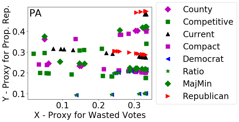
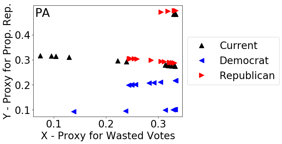
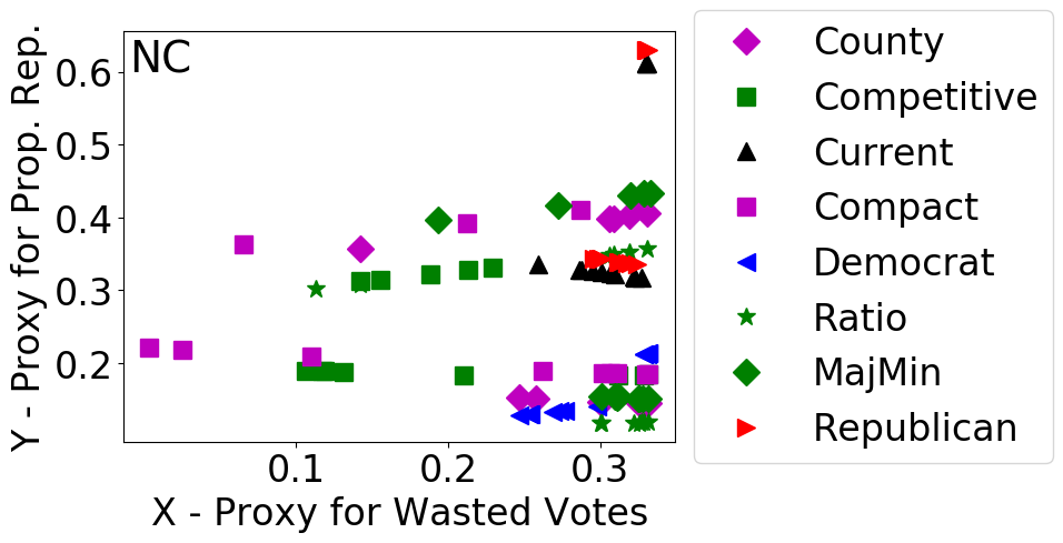
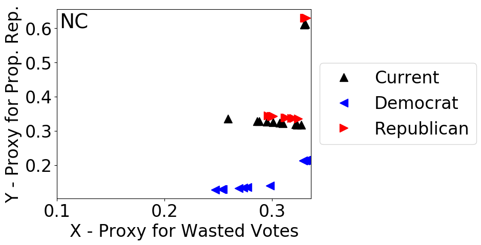
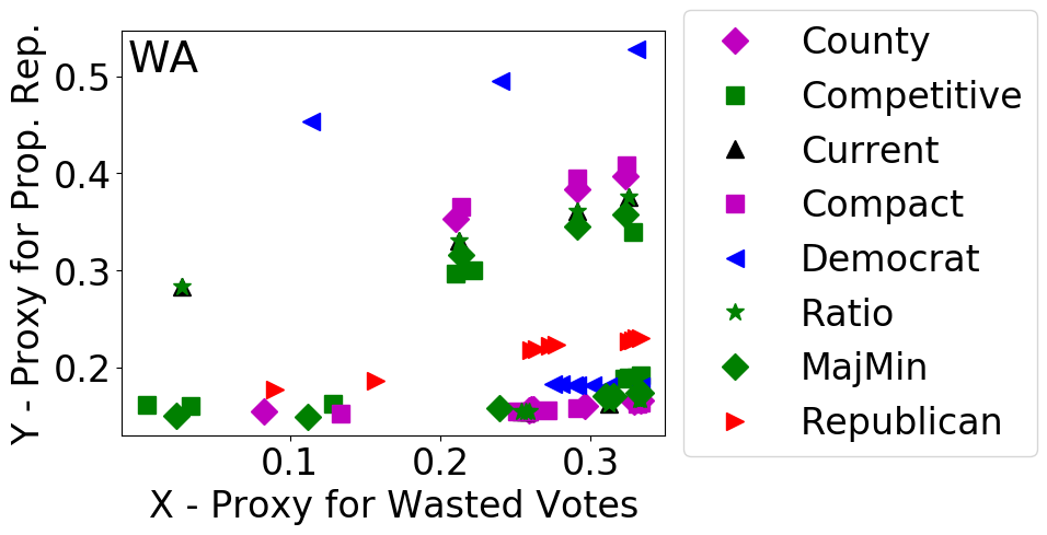
Figure 1: Characteristic data for Pennsylvania, North Carolina, and Washington.

Consider the graph for North Carolina in Figure 1 that illustrates the current, Republican, and Democratic maps, for which the proximity measures are respectively $0.1680$, $0.0932$, and $0.0294$. The Democratic map has the lowest proximity value of the three even though its districts trend toward the lower right portion of the graph, which might seem to suggest that the current and Republican maps are better. However, both the current and Republican maps have districts near the top and/or left of the graph that are somewhat distant from other districts toward the bottom and/or right, and this spread between their best and worst districts increases the value of the proximity to equitable efficiency. The proximity values for the current and Republican maps are higher than that of the Democratic map because they require more characteristic uncertainty before all districts have an equal claim to efficiency with regard to each other. This fact is important to note: the proximity to equitable efficiency is an intra-comparison and not an inter-comparison, and a map’s proximity to equitable efficiency is indifferent to the other maps. In this case, the districts of the Democratic map are more equitable, especially with regard to their role in proportional representation, than are the districts of either the current or Republican map. An apt interpretation is that the high quality districts of the current and Republican maps force the other districts to have less quality with regard to efficiency, and it is this disparity that the proximity to equitable efficiency measures. A similar analysis applies to the comparison of the current, Republican, and Democratic maps of Washington, but in this case the Republican map’s proximity value of $0.0192$ bests those of the current and Democratic maps, which are $0.2385$ and $0.1864$. A graphical interpretation of Pennsylvania is less clear, and in this case the proximity values are $0.182$ (current), $0.1194$ (Republican), and $0.1342$ (Democratic). Conspicuous disparities in this case appear, at least primarily, to be the result of variations with regard to wasted votes.

We remind that our proximity measure does not specifically favor a map because its districts have more homogeneous characteristics. This suspicion would in fact be a misinterpretation of the results just presented. For instance, it is incorrect to assume that the Republican map for Washington is favored by our proximity measure simply because its data is most clustered. The Wisconsin map in Figure 2 illustrates this point by adding the traditional efficient frontiers of each map. A map’s proximity value is zero only if all districts lie on their respective efficient frontier. The Republican map in this case has the lowest proximity measure although its data has a greater spread of proportional representation and about an equal spread of wasted votes as compared with the Democratic map. To exaggerate this point, suppose that the current map’s districts to the lower right had instead appeared on their (black) efficient frontier. The current map would have then had a proximity value of zero, and it would have been preferred over both the Democratic and Republican maps even though its districts would have had a far greater variation in their characteristics. Lastly, our proximity measure is also not a straightforward merger of distances from the efficient frontier because the frontier itself depends on how each district individually selects data from the realm of uncertain options.

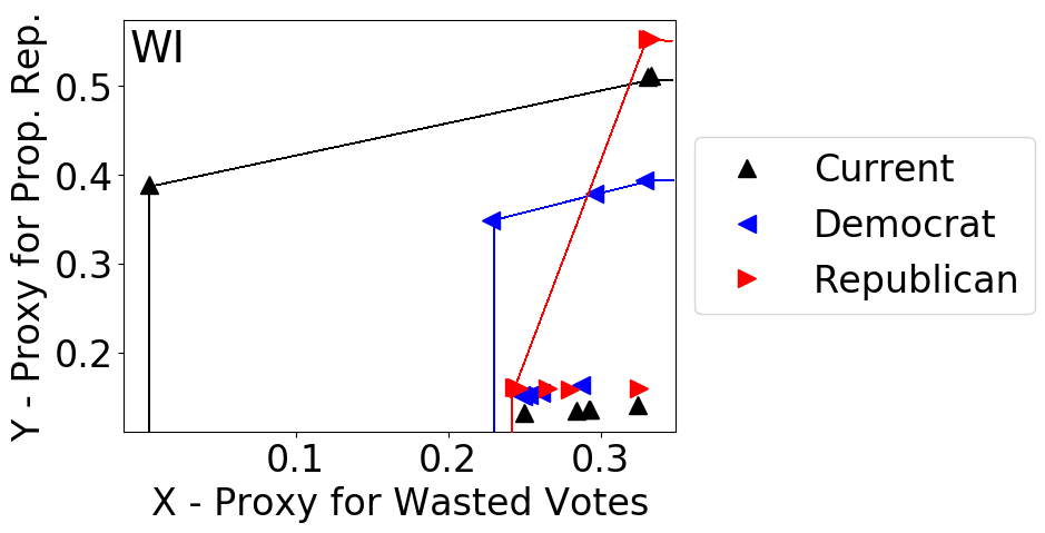
Figure 2: Wisconsin’s Democratic, Republican, and current maps with original efficient frontiers.

The results of this section can be recreated with the supplemental python code, which is described in the supplementary material. This code could be altered to replace or add new characteristics or to assess newly proposed congressional maps. All robust problems were modeled with Pyomo [13] and solved with Gurobi.

Supplmentary Materials for
Comparing Voting Districts with
Uncertain Data Envelopment Analysis

1 Software

Python code to reproduce the results in Using Uncertain Data Envelopment Analysis to Compare Classifications with an Application in Gerrymandering is part of the supplementary materials. Data is located in the data directory with the following titles:

• CongressionalDistricts.txt - original source data from FiveThirtyEight’s The Atlas of Redistricting,

• partyAffiliation.csv – original source data from the Pew Research Center,

• XdataFile.dat.article – transformed data $X_{skt}$,

• YdataFile.dat.article – transformed data $Y_{skt}$,

• gmResultsStateMap.csv – results in Table LABEL:table-completeResults in Section 2, and

• gmResultsState.csv – results for all states like those in Table 1 of the article.

Python code is in the ver1 directory, with the primary script being

gerrymandering.py.

The code runs with Python 2.7.17 and requires Pyomo [13] and Gurobi. Settings at the top of gerrymandering.py allow a user to set the states and maps to consider, to generate new data ($Y_{skt}$), to save data, to generate new LaTeX tables, and to make new data plots like those in Figure 1. New figures are placed in the figs directory in png format. Completing the script with the article’s data takes several hours, and simulating new data takes about an hour.

2 Complete Tabulated Results

Table LABEL:table-completeResults lists comparative results for all state and map combinations. The state order decreases in the number of congressional districts, and each value of ${\cal P}({\cal C})$ is either bounded $\hat{\sigma}$ or is stated as an equality.

Table 2: Complete results listing all state and map combinations.

	Num.	Most	$\mathcal{P}(\mathcal{C})=\|\hat{\sigma}\|$
	of	Proximal	or	optimal $\sigma^{*}$
State	Dist.	Map	$\|\hat{\sigma}\|/\sqrt{2}\leq\mathcal{P}(\mathcal{C})\leq\|\hat{\sigma}\|$	$\sigma^{*}_{X}$	$\sigma^{*}_{Y}$
CA	53	Cty	$0.1152\leq 0.1629\leq 0.1630$	$0.0866$	$0.1380$
CA	53	Cpt	$0.1131\leq 0.1599\leq 0.1600$	$0.1233$	$0.1018$
CA	53	Crt	$0.1361\leq 0.1361\leq 0.1926$	$0.0992$	$0.0932$
CA	53	Cmt	$0.1007\leq 0.1424\leq 0.1424$	$0.0877$	$0.1121$
CA	53	Dem	$0.0954\leq 0.0954\leq 0.1350$	$0.0669$	$0.0680$
CA	53	Rto	$0.0606\leq 0.0857\leq 0.0857$	$0.0334$	$0.0789$
CA	53	MMn	$0.1326\leq 0.1326\leq 0.1876$	$0.0975$	$0.0899$
CA	53	Rep	$0.0697\leq 0.0986\leq 0.0986$	$0.0510$	$0.0843$
TX	36	Cty	$0.1733\leq 0.2451\leq 0.2451$	$0.1947$	$0.1489$
TX	36	Cpt	$0.1369\leq 0.1935\leq 0.1936$	$0.1371$	$0.1365$
TX	36	Crt	$0.1222\leq 0.1222\leq 0.1728$	$0.0195$	$0.1206$
TX	36	Cmt	$0.1751\leq 0.1751\leq 0.2478$	$0.1125$	$0.1342$
TX	36	Dem	$0.0969\leq 0.0969\leq 0.1371$	$0.0622$	$0.0743$
TX	36	Rto	$0.1396\leq 0.1974\leq 0.1975$	$0.1321$	$0.1467$
TX	36	MMn	$0.1314\leq 0.1314\leq 0.1859$	$0.0632$	$0.1152$
TX	36	Rep	$0.1505\leq 0.1505\leq 0.2130$	$0.1157$	$0.0962$
FL	27	Cty	$0.1481\leq 0.1481\leq 0.2095$	$0.0900$	$0.1176$
FL	27	Cpt	$0.1369\leq 0.1369\leq 0.1937$	$0.0858$	$0.1067$
FL	27	Crt	$0.1417\leq 0.2003\leq 0.2004$	$0.1439$	$0.1393$
FL	27	Cmt	$0.1424\leq 0.2013\leq 0.2014$	$0.1507$	$0.1334$
FL	27	Dem	$0.0870\leq 0.0870\leq 0.1231$	$0.0607$	$0.0624$
FL	27	Rto	$0.1198\leq 0.1198\leq 0.1695$	$-0.0071$	$0.1196$
FL	27	MMn	$0.1530\leq 0.2163\leq 0.2163$	$0.1435$	$0.1618$
FL	27	Rep	$0.1515\leq 0.1515\leq 0.2143$	$0.1029$	$0.1111$
NY	27	Cty	$0.1396\leq 0.1974\leq 0.1975$	$0.1363$	$0.1427$
NY	27	Cpt	$0.1618=0.1618$	$0.1130$	$0.1157$
NY	27	Crt	$0.1820\leq 0.2573\leq 0.2573$	$0.2043$	$0.1564$
NY	27	Cmt	$0.1535\leq 0.1535\leq 0.2172$	$0.0915$	$0.1232$
NY	27	Dem	$0.1474\leq 0.2084\leq 0.2085$	$0.1879$	$0.0901$
NY	27	Rto	$0.1723\leq 0.2436\leq 0.2437$	$0.1587$	$0.1848$
NY	27	MMn	$0.1528\leq 0.2160\leq 0.2161$	$0.1290$	$0.1733$
NY	27	Rep	$0.0155\leq 0.0219\leq 0.0220$	$0.0144$	$0.0165$
PA	18	Cty	$0.2129\leq 0.2129\leq 0.3011$	$0.1349$	$0.1646$
PA	18	Cpt	$0.1672\leq 0.2364\leq 0.2365$	$0.1569$	$0.1768$
PA	18	Crt	$0.1824\leq 0.1824\leq 0.2580$	$0.1378$	$0.1194$
PA	18	Cmt	$0.2058\leq 0.2909\leq 0.2910$	$0.1924$	$0.2182$
PA	18	Dem	$0.1342\leq 0.1342\leq 0.1899$	$0.0968$	$0.0930$
PA	18	Rto	$0.1342\leq 0.1342\leq 0.1899$	$0.0968$	$0.0930$
PA	18	MMn	$0.2254\leq 0.2254\leq 0.3188$	$0.1849$	$0.1288$
PA	18	Rep	$0.1193\leq 0.1193\leq 0.1688$	$0.0535$	$0.1066$
IL	18	Cty	$0.0942\leq 0.0942\leq 0.1333$	$0.0508$	$0.0793$
IL	18	Cpt	$0.0981\leq 0.1386\leq 0.1387$	$0.0905$	$0.1050$
IL	18	Crt	$0.1427\leq 0.2017\leq 0.2018$	$0.1361$	$0.1488$
IL	18	Cmt	$0.1032=0.1032$	$0.0898$	$0.0507$
IL	18	Dem	$0.1357\leq 0.1357\leq 0.1920$	$0.1048$	$0.0861$
IL	18	Rto	$0.0974\leq 0.0974\leq 0.1379$	$0.0781$	$0.0582$
IL	18	MMn	$0.1018=0.1018$	$0.0600$	$0.0822$
IL	18	Rep	$0.0813\leq 0.0813\leq 0.1150$	$0.0644$	$0.0495$
OH	16	Cty	$0.2328\leq 0.3291\leq 0.3292$	$0.2756$	$0.1798$
OH	16	Cpt	$0.1685\leq 0.2382\leq 0.2383$	$0.1709$	$0.1660$
OH	16	Crt	$0.1738\leq 0.1738\leq 0.2459$	$0.0978$	$0.1436$
OH	16	Cmt	$0.2593\leq 0.3666\leq 0.3667$	$0.3194$	$0.1799$
OH	16	Dem	$0.1564=0.1564$	$0.1185$	$0.1020$
OH	16	Rto	$0.0910\leq 0.0910\leq 0.1288$	$0.0711$	$0.0568$
OH	16	MMn	$0.2010\leq 0.2842\leq 0.2843$	$0.2413$	$0.1500$
OH	16	Rep	$0.0972\leq 0.1373\leq 0.1374$	$0.0805$	$0.1112$
GA	14	Cty	$0.1654\leq 0.2338\leq 0.2338$	$0.2208$	$0.0768$
GA	14	Cpt	$0.1790\leq 0.2530\leq 0.2531$	$0.1794$	$0.1784$
GA	14	Crt	$0.0880\leq 0.0880\leq 0.1246$	$0.0849$	$0.0232$
GA	14	Cmt	$0.1643\leq 0.2323\leq 0.2323$	$0.2270$	$0.0494$
GA	14	Dem	$0.0686\leq 0.0970\leq 0.0971$	$0.0670$	$0.0701$
GA	14	Rto	$0.1066\leq 0.1507\leq 0.1507$	$0.1398$	$0.0561$
GA	14	MMn	$0.1744\leq 0.2466\leq 0.2467$	$0.2385$	$0.0626$
GA	14	Rep	$0.0633\leq 0.0633\leq 0.0896$	$0.0325$	$0.0543$
MI	14	Cty	$0.2106\leq 0.2978\leq 0.2979$	$0.2357$	$0.1820$
MI	14	Cpt	$0.1864\leq 0.1864\leq 0.2637$	$0.1123$	$0.1487$
MI	14	Crt	$0.1277\leq 0.1277\leq 0.1807$	$0.1013$	$0.0777$
MI	14	Cmt	$0.1878\leq 0.2654\leq 0.2655$	$0.1847$	$0.1906$
MI	14	Dem	$0.0640\leq 0.0904\leq 0.0905$	$0.0775$	$0.0465$
MI	14	Rto	$0.1178=0.1178$	$0.1024$	$0.0582$
MI	14	MMn	$0.1340\leq 0.1340\leq 0.1896$	$0.1063$	$0.0816$
MI	14	Rep	$0.0770\leq 0.1088\leq 0.1089$	$0.0818$	$0.0717$
NC	13	Cty	$0.1647\leq 0.1647\leq 0.2330$	$0.1632$	$0.0224$
NC	13	Cpt	$0.2536=0.2536$	$0.1680$	$0.1899$
NC	13	Crt	$0.1188\leq 0.1680\leq 0.1680$	$0.1116$	$0.1255$
NC	13	Cmt	$0.1991\leq 0.2814\leq 0.2815$	$0.2180$	$0.1779$
NC	13	Dem	$0.0294\leq 0.0294\leq 0.0416$	$0.0178$	$0.0234$
NC	13	Rto	$0.2110\leq 0.2110\leq 0.2984$	$0.1804$	$0.1093$
NC	13	MMn	$0.1530\leq 0.1530\leq 0.2164$	$0.1372$	$0.0677$
NC	13	Rep	$0.0660\leq 0.0932\leq 0.0933$	$0.0545$	$0.0756$
NJ	12	Cty	$0.1961\leq 0.1961\leq 0.2774$	$0.1537$	$0.1218$
NJ	12	Cpt	$0.1328\leq 0.1877\leq 0.1878$	$0.1509$	$0.1117$
NJ	12	Crt	$0.1359=0.1359$	$0.1038$	$0.0878$
NJ	12	Cmt	$0.1612\leq 0.2279\leq 0.2280$	$0.1583$	$0.1639$
NJ	12	Dem	$0.0862\leq 0.1218\leq 0.1219$	$0.0870$	$0.0852$
NJ	12	Rto	$0.1540\leq 0.1540\leq 0.2179$	$0.1038$	$0.1138$
NJ	12	MMn	$0.1237\leq 0.1237\leq 0.1751$	$0.0827$	$0.0920$
NJ	12	Rep	$0.0762=0.0762$	$0.0099$	$0.0755$
VA	11	Cty	$0.0651\leq 0.0651\leq 0.0921$	$0.0504$	$0.0412$
VA	11	Cpt	$0.1883=0.1883$	$0.1345$	$0.1317$
VA	11	Crt	$0.0851\leq 0.0851\leq 0.1205$	$0.0651$	$0.0548$
VA	11	Cmt	$0.1021\leq 0.1021\leq 0.1445$	$0.0599$	$0.0827$
VA	11	Dem	$0.0999\leq 0.1412\leq 0.1413$	$0.1101$	$0.0884$
VA	11	Rto	$0.1112\leq 0.1112\leq 0.1573$	$0.0811$	$0.0760$
VA	11	MMn	$0.0651\leq 0.0920\leq 0.0920$	$0.0874$	$0.0285$
VA	11	Rep	$0.0934\leq 0.1320\leq 0.1321$	$0.1110$	$0.0715$
WA	10	Cty	$0.1546\leq 0.2186\leq 0.2187$	$0.1396$	$0.1682$
WA	10	Cpt	$0.1563\leq 0.1563\leq 0.2212$	$0.0995$	$0.1206$
WA	10	Crt	$0.1687\leq 0.2385\leq 0.2386$	$0.1772$	$0.1595$
WA	10	Cmt	$0.1667\leq 0.2357\leq 0.2357$	$0.1353$	$0.1929$
WA	10	Dem	$0.1864\leq 0.1864\leq 0.2637$	$0.1776$	$0.0567$
WA	10	Rto	$0.1995\leq 0.2820\leq 0.2821$	$0.2322$	$0.1601$
WA	10	MMn	$0.1596\leq 0.1596\leq 0.2258$	$0.1091$	$0.1165$
WA	10	Rep	$0.0136\leq 0.0192\leq 0.0193$	$0.0183$	$0.0056$
TN	9	Cty	$0.1559=0.1559$	$0.1380$	$0.0726$
TN	9	Cpt	$0.1986=0.1986$	$0.1884$	$0.0628$
TN	9	Crt	$0.0826\leq 0.1167\leq 0.1168$	$0.1167$	$0.0032$
TN	9	Cmt	$0.1365\leq 0.1365\leq 0.1930$	$0.0884$	$0.1039$
TN	9	Dem	$0.1061\leq 0.1061\leq 0.1501$	$0.1061$	$0.0000$
TN	9	Rto	$0.2480\leq 0.3506\leq 0.3507$	$0.3506$	$0.0000$
TN	9	MMn	$0.0862\leq 0.1219\leq 0.1219$	$0.1218$	$0.0032$
TN	9	Rep	$0.0287\leq 0.0287\leq 0.0406$	$0.0284$	$0.0034$
IN	9	Cty	$0.0619\leq 0.0619\leq 0.0876$	$0.0443$	$0.0432$
IN	9	Cpt	$0.1825\leq 0.1825\leq 0.2582$	$0.1716$	$0.0622$
IN	9	Crt	$0.1133=0.1133$	$0.1023$	$0.0487$
IN	9	Cmt	$0.1032\leq 0.1032\leq 0.1460$	$0.1011$	$0.0205$
IN	9	Dem	$0.1212\leq 0.1713\leq 0.1714$	$0.1597$	$0.0620$
IN	9	Rto	$0.3227=0.3227$	$0.2966$	$0.1271$
IN	9	MMn	$0.0693\leq 0.0979\leq 0.0980$	$0.0634$	$0.0746$
IN	9	Rep	$0.0195\leq 0.0195\leq 0.0276$	$0.0090$	$0.0172$
MA	9	Cty	$0.0585\leq 0.0585\leq 0.0828$	$0.0126$	$0.0571$
MA	9	Cpt	$0.1758\leq 0.2486\leq 0.2486$	$0.2479$	$0.0186$
MA	9	Crt	$0.0504\leq 0.0711\leq 0.0712$	$0.0459$	$0.0543$
MA	9	Cmt	$0.0684=0.0684$	$0.0491$	$0.0475$
MA	9	Dem	$0.0317\leq 0.0448\leq 0.0448$	$0.0244$	$0.0375$
MA	9	Rto	$0.2899\leq 0.4099\leq 0.4100$	$0.3522$	$0.2098$
MA	9	MMn	$0.0505\leq 0.0713\leq 0.0714$	$0.0460$	$0.0544$
MA	9	Rep	$0.2239=0.2239$	$0.2190$	$0.0464$
AZ	9	Cty	$0.1372\leq 0.1372\leq 0.1941$	$0.1015$	$0.0923$
AZ	9	Cpt	$0.1042\leq 0.1042\leq 0.1474$	$0.0683$	$0.0787$
AZ	9	Crt	$0.1779\leq 0.2515\leq 0.2516$	$0.1871$	$0.1680$
AZ	9	Cmt	$0.2077\leq 0.2937\leq 0.2938$	$0.2007$	$0.2143$
AZ	9	Dem	$0.0718\leq 0.1014\leq 0.1015$	$0.0643$	$0.0784$
AZ	9	Rto	$0.1621\leq 0.2292\leq 0.2293$	$0.2204$	$0.0627$
AZ	9	MMn	$0.1917\leq 0.2711\leq 0.2711$	$0.2021$	$0.1807$
AZ	9	Rep	$0.0806\leq 0.1139\leq 0.1140$	$0.0750$	$0.0858$
WI	8	Cty	$0.1523\leq 0.2154\leq 0.2154$	$0.1388$	$0.1647$
WI	8	Cpt	$0.1833\leq 0.1833\leq 0.2593$	$0.1262$	$0.1329$
WI	8	Crt	$0.2022\leq 0.2858\leq 0.2859$	$0.2441$	$0.1487$
WI	8	Cmt	$0.2013=0.2013$	$0.1989$	$0.0309$
WI	8	Dem	$0.1010\leq 0.1010\leq 0.1429$	$0.0999$	$0.0151$
WI	8	Rto	$0.2270\leq 0.2270\leq 0.3211$	$0.1537$	$0.1670$
WI	8	MMn	$0.1965\leq 0.1965\leq 0.2779$	$0.1372$	$0.1406$
WI	8	Rep	$0.0987=0.0987$	$0.0686$	$0.0710$
MD	8	Cty	$0.2107\leq 0.2980\leq 0.2980$	$0.2106$	$0.2108$
MD	8	Cpt	$0.1637=0.1637$	$0.0360$	$0.1597$
MD	8	Crt	$0.0678\leq 0.0678\leq 0.0959$	$0.0583$	$0.0345$
MD	8	Cmt	$0.1549=0.1549$	$0.1090$	$0.1101$
MD	8	Dem	$0.0417\leq 0.0590\leq 0.0590$	$0.0384$	$0.0447$
MD	8	Rto	$0.1533\leq 0.2167\leq 0.2168$	$0.1844$	$0.1138$
MD	8	MMn	$0.0833=0.0833$	$0.0524$	$0.0647$
MD	8	Rep	$0.0939=0.0939$	$0.0623$	$0.0703$
MO	8	Cty	$0.2369\leq 0.3349\leq 0.3350$	$0.3241$	$0.0843$
MO	8	Cpt	$0.1051\leq 0.1486\leq 0.1487$	$0.1458$	$0.0284$
MO	8	Crt	$0.0448\leq 0.0448\leq 0.0635$	$0.0422$	$0.0151$
MO	8	Cmt	$0.1299=0.1299$	$0.1195$	$0.0508$
MO	8	Dem	$0.0498\leq 0.0703\leq 0.0704$	$0.0659$	$0.0245$
MO	8	Rto	$0.1109\leq 0.1109\leq 0.1569$	$0.1094$	$0.0179$
MO	8	MMn	$0.0448\leq 0.0448\leq 0.0635$	$0.0422$	$0.0151$
MO	8	Rep	$0.1420=0.1420$	$0.0929$	$0.1073$
MN	8	Cty	$0.1455\leq 0.2058\leq 0.2058$	$0.1448$	$0.1461$
MN	8	Cpt	$0.1877\leq 0.2653\leq 0.2654$	$0.2323$	$0.1282$
MN	8	Crt	$0.1706\leq 0.2413\leq 0.2413$	$0.2304$	$0.0717$
MN	8	Cmt	$0.1429\leq 0.2021\leq 0.2021$	$0.1289$	$0.1556$
MN	8	Dem	$0.0677\leq 0.0677\leq 0.0958$	$0.0603$	$0.0306$
MN	8	Rto	$0.1936=0.1936$	$0.1391$	$0.1346$
MN	8	MMn	$0.1790\leq 0.2531\leq 0.2532$	$0.2320$	$0.1011$
MN	8	Rep	$0.1294=0.1294$	$0.0911$	$0.0918$
CO	7	Cty	$0.0984\leq 0.1391\leq 0.1391$	$0.1157$	$0.0771$
CO	7	Cpt	$0.1055\leq 0.1055\leq 0.1492$	$0.0715$	$0.0775$
CO	7	Crt	$0.1015=0.1015$	$0.0711$	$0.0724$
CO	7	Cmt	$0.1013\leq 0.1432\leq 0.1433$	$0.0987$	$0.1037$
CO	7	Dem	$0.1255\leq 0.1255\leq 0.1775$	$0.1231$	$0.0245$
CO	7	Rto	$0.0732\leq 0.1035\leq 0.1035$	$0.0761$	$0.0701$
CO	7	MMn	$0.1114=0.1114$	$0.1012$	$0.0467$
CO	7	Rep	$0.0678\leq 0.0678\leq 0.0960$	$0.0492$	$0.0466$
AL	7	Cty	$0.2479\leq 0.3505\leq 0.3505$	$0.3504$	$0.0039$
AL	7	Cpt	$0.1882\leq 0.2661\leq 0.2662$	$0.2436$	$0.1071$
AL	7	Crt	$0.0067\leq 0.0095\leq 0.0095$	$0.0095$	$0.0000$
AL	7	Cmt	$0.0899\leq 0.1270\leq 0.1271$	$0.0694$	$0.1064$
AL	7	Dem	$0.0590=0.0590$	$0.0541$	$0.0234$
AL	7	Rto	$0.0584=0.0584$	$0.0531$	$0.0243$
AL	7	MMn	$0.0590=0.0590$	$0.0541$	$0.0234$
AL	7	Rep	$0.0067\leq 0.0095\leq 0.0095$	$0.0095$	$0.0000$
SC	7	Cty	$0.2099\leq 0.2967\leq 0.2968$	$0.2816$	$0.0934$
SC	7	Cpt	$0.2909=0.2909$	$0.2589$	$0.1326$
SC	7	Crt	$0.0248=0.0248$	$0.0245$	$0.0037$
SC	7	Cmt	$0.0930\leq 0.0930\leq 0.1316$	$0.0893$	$0.0259$
SC	7	Dem	$0.1672=0.1672$	$0.1588$	$0.0524$
SC	7	Rto	$0.2909=0.2909$	$0.2589$	$0.1326$
SC	7	MMn	$0.0234\leq 0.0234\leq 0.0332$	$0.0234$	$0.0000$
SC	7	Rep	$0.0248=0.0248$	$0.0245$	$0.0037$
LA	6	Cty	$0.1220=0.1220$	$0.1200$	$0.0218$
LA	6	Cpt	$0.1523\leq 0.2154\leq 0.2154$	$0.2146$	$0.0180$
LA	6	Crt	$0.0068\leq 0.0096\leq 0.0097$	$0.0096$	$0.0003$
LA	6	Cmt	$0.0904\leq 0.1278\leq 0.1278$	$0.0885$	$0.0921$
LA	6	Dem	$0.0977\leq 0.0977\leq 0.1382$	$0.0976$	$-0.0051$
LA	6	Rto	$0.0977\leq 0.0977\leq 0.1382$	$0.0976$	$-0.0051$
LA	6	MMn	$0.0957\leq 0.0957\leq 0.1353$	$0.0953$	$0.0080$
LA	6	Rep	$0.0068\leq 0.0096\leq 0.0097$	$0.0096$	$0.0003$
KY	6	Cty	$0.0687=0.0687$	$0.0601$	$0.0334$
KY	6	Cpt	$0.2263\leq 0.2263\leq 0.3201$	$0.2194$	$0.0551$
KY	6	Crt	$0.1064\leq 0.1064\leq 0.1505$	$0.1062$	$0.0072$
KY	6	Cmt	$0.1159=0.1159$	$0.1093$	$0.0384$
KY	6	Dem	$0.0564\leq 0.0797\leq 0.0797$	$0.0790$	$0.0105$
KY	6	Rto	$0.2096\leq 0.2963\leq 0.2964$	$0.2963$	$0.0000$
KY	6	MMn	$0.0941\leq 0.1331\leq 0.1331$	$0.1179$	$0.0616$
KY	6	Rep	$0.0393\leq 0.0556\leq 0.0556$	$0.0360$	$0.0423$
CT	5	Cty	$0.1184\leq 0.1673\leq 0.1674$	$0.1533$	$0.0670$
CT	5	Cpt	$0.1909=0.1909$	$0.1533$	$0.1137$
CT	5	Crt	$0.0360\leq 0.0360\leq 0.0510$	$0.0053$	$0.0356$
CT	5	Cmt	$0.0953\leq 0.1347\leq 0.1348$	$0.1332$	$0.0199$
CT	5	Dem	$0.0167\leq 0.0167\leq 0.0236$	$0.0065$	$0.0153$
CT	5	Rto	$0.2389\leq 0.3377\leq 0.3378$	$0.3066$	$0.1415$
CT	5	MMn	$0.1512\leq 0.2137\leq 0.2138$	$0.1945$	$0.0886$
CT	5	Rep	$0.2149=0.2149$	$0.1519$	$0.1519$
OK	5	Cty	$0.0259\leq 0.0259\leq 0.0367$	$0.0188$	$0.0179$
OK	5	Cpt	$0.0863\leq 0.1220\leq 0.1221$	$0.0673$	$0.1017$
OK	5	Crt	$0.0831=0.0831$	$0.0565$	$0.0609$
OK	5	Cmt	$0.0825=0.0825$	$0.0506$	$0.0652$
OK	5	Dem	$0.1683\leq 0.2379\leq 0.2380$	$0.2035$	$0.1232$
OK	5	Rto	$0.2245=0.2245$	$0.2035$	$0.0946$
OK	5	MMn	$0.0968\leq 0.1368\leq 0.1369$	$0.0914$	$0.1018$
OK	5	Rep	$0.0831=0.0831$	$0.0565$	$0.0609$
OR	5	Cty	$0.1007=0.1007$	$0.0700$	$0.0723$
OR	5	Cpt	$0.0654\leq 0.0654\leq 0.0925$	$0.0134$	$0.0640$
OR	5	Crt	$0.1131=0.1131$	$0.0798$	$0.0801$
OR	5	Cmt	$0.0648\leq 0.0648\leq 0.0918$	$0.0043$	$0.0647$
OR	5	Dem	$0.1198=0.1198$	$0.0848$	$0.0845$
OR	5	Rto	$0.1250=0.1250$	$0.0761$	$0.0992$
OR	5	MMn	$0.0687=0.0687$	$0.0658$	$0.0197$
OR	5	Rep	$0.0052\leq 0.0052\leq 0.0074$	$0.0038$	$0.0035$
NV	4	Cty	$0.1745=0.1745$	$0.0587$	$0.1643$
NV	4	Cpt	$0.0294=0.0294$	$0.0167$	$0.0242$
NV	4	Crt	$0.1009=0.1009$	$0.0712$	$0.0715$
NV	4	Cmt	$0.1069=0.1069$	$0.0143$	$0.1060$
NV	4	Dem	$0.0358=0.0358$	$0.0358$	$0.0000$
NV	4	Rto	$0.1094=0.1094$	$0.0848$	$0.0690$
NV	4	MMn	$0.0193\leq 0.0193\leq 0.0273$	$0.0193$	$0.0000$
NV	4	Rep	$0.1433=0.1433$	$0.1397$	$0.0319$
AR	4	Cty	$0.0285=0.0285$	$0.0007$	$0.0285$
AR	4	Cpt	$0.1778\leq 0.2514\leq 0.2515$	$0.2509$	$0.0162$
AR	4	Crt	$0.0345\leq 0.0345\leq 0.0489$	$0.0307$	$0.0158$
AR	4	Cmt	$0.0447=0.0447$	$0.0304$	$0.0327$
AR	4	Dem	$0.1160\leq 0.1160\leq 0.1642$	$0.1155$	$0.0108$
AR	4	Rto	$0.1226\leq 0.1226\leq 0.1734$	$0.1163$	$0.0386$
AR	4	MMn	$0.0362\leq 0.0362\leq 0.0513$	$0.0362$	$0.0000$
AR	4	Rep	$0.0345\leq 0.0345\leq 0.0489$	$0.0307$	$0.0158$
IA	4	Cty	$0.0383\leq 0.0541\leq 0.0542$	$0.0466$	$0.0275$
IA	4	Cpt	$0.0359\leq 0.0507\leq 0.0507$	$0.0455$	$0.0223$
IA	4	Crt	$0.1002=0.1002$	$0.0819$	$0.0576$
IA	4	Cmt	$0.0933=0.0933$	$0.0820$	$0.0445$
IA	4	Dem	$0.1433=0.1433$	$0.1013$	$0.1013$
IA	4	Rto	$0.0359\leq 0.0507\leq 0.0507$	$0.0455$	$0.0223$
IA	4	MMn	$0.1658\leq 0.2344\leq 0.2344$	$0.2337$	$0.0183$
IA	4	Rep	$0.0553\leq 0.0781\leq 0.0782$	$0.0557$	$0.0547$
UT	4	Cty	$0.1011=0.1011$	$0.1008$	$0.0077$
UT	4	Cpt	$0.1011=0.1011$	$0.1008$	$0.0077$
UT	4	Crt	$0.0052\leq 0.0052\leq 0.0074$	$0.0031$	$0.0041$
UT	4	Cmt	$0.1679=0.1679$	$0.1230$	$0.1142$
UT	4	Dem	$0.0695=0.0695$	$0.0613$	$0.0326$
UT	4	Rto	$0.0695=0.0695$	$0.0613$	$0.0326$
UT	4	MMn	$0.0887=0.0887$	$0.0852$	$0.0246$
UT	4	Rep	$0.0052\leq 0.0052\leq 0.0074$	$0.0031$	$0.0041$
KS	4	Cty	$0.0349\leq 0.0349\leq 0.0494$	$0.0046$	$0.0346$
KS	4	Cpt	$0.0109\leq 0.0154\leq 0.0155$	$0.0099$	$0.0118$
KS	4	Crt	$0.0386\leq 0.0545\leq 0.0546$	$0.0345$	$0.0422$
KS	4	Cmt	$0.0412\leq 0.0583\leq 0.0583$	$0.0394$	$0.0428$
KS	4	Dem	$0.0878\leq 0.1242\leq 0.1242$	$0.0964$	$0.0782$
KS	4	Rto	$0.1763\leq 0.1763\leq 0.2494$	$0.1762$	$0.0055$
KS	4	MMn	$0.1472\leq 0.2081\leq 0.2082$	$0.2080$	$0.0063$
KS	4	Rep	$0.0686=0.0686$	$0.0622$	$0.0287$
MS	4	Cty	$0.1141\leq 0.1613\leq 0.1614$	$0.1568$	$0.0379$
MS	4	Cpt	$0.1617\leq 0.2287\leq 0.2287$	$0.2286$	$0.0035$
MS	4	Crt	$0.0072\leq 0.0101\leq 0.0102$	$0.0099$	$0.0022$
MS	4	Cmt	$0.1276=0.1276$	$0.1255$	$0.0229$
MS	4	Dem	$0.0976=0.0976$	$0.0976$	$0.0000$
MS	4	Rto	$0.1617\leq 0.2287\leq 0.2287$	$0.2286$	$0.0035$
MS	4	MMn	$0.0853\leq 0.1206\leq 0.1206$	$0.0594$	$0.1049$
MS	4	Rep	$0.0072\leq 0.0101\leq 0.0102$	$0.0099$	$0.0022$
WV	3	Cty	$0.0070=0.0070$	$0.0043$	$0.0055$
WV	3	Cpt	$0.0033\leq 0.0033\leq 0.0048$	$0.0000$	$0.0033$
WV	3	Crt	$0.0049\leq 0.0049\leq 0.0070$	$0.0027$	$0.0041$
WV	3	Cmt	$0.0067=0.0067$	$0.0060$	$0.0030$
WV	3	Dem	$0.0033\leq 0.0033\leq 0.0048$	$0.0000$	$0.0033$
WV	3	Rto	$0.0033\leq 0.0033\leq 0.0048$	$0.0000$	$0.0033$
WV	3	MMn	$0.0033\leq 0.0033\leq 0.0048$	$0.0000$	$0.0033$
WV	3	Rep	$0.0049\leq 0.0049\leq 0.0070$	$0.0027$	$0.0041$
NM	3	Cty	$0.0927=0.0927$	$0.0025$	$0.0927$
NM	3	Cpt	$0.0000=0.0000$	$0.0000$	$0.0000$
NM	3	Crt	$0.0000=0.0000$	$0.0000$	$0.0000$
NM	3	Cmt	$0.0000=0.0000$	$0.0000$	$0.0000$
NM	3	Dem	$0.0000=0.0000$	$0.0000$	$0.0000$
NM	3	Rto	$0.0000=0.0000$	$0.0000$	$0.0000$
NM	3	MMn	$0.0035=0.0035$	$0.0035$	$0.0000$
NM	3	Rep	$0.0196=0.0196$	$0.0139$	$0.0139$
NE	3	Cty	$0.0070=0.0070$	$0.0050$	$0.0049$
NE	3	Cpt	$0.0064=0.0064$	$0.0024$	$0.0060$
NE	3	Crt	$0.0070=0.0070$	$0.0055$	$0.0042$
NE	3	Cmt	$0.0046=0.0046$	$0.0000$	$0.0046$
NE	3	Dem	$0.0231\leq 0.0326\leq 0.0326$	$0.0214$	$0.0245$
NE	3	Rto	$0.0231\leq 0.0326\leq 0.0326$	$0.0214$	$0.0245$
NE	3	MMn	$0.0050=0.0050$	$0.0000$	$0.0050$
NE	3	Rep	$0.0028\leq 0.0028\leq 0.0040$	$0.0009$	$0.0026$
HI	2	Cty	$0.0000=0.0000$	$0.0000$	$0.0000$
HI	2	Cpt	$0.0000=0.0000$	$0.0000$	$0.0000$
HI	2	Crt	$0.0000=0.0000$	$0.0000$	$0.0000$
HI	2	Cmt	$0.0000=0.0000$	$0.0000$	$0.0000$
HI	2	Dem	$0.0000=0.0000$	$0.0000$	$0.0000$
HI	2	Rto	$0.0000=0.0000$	$0.0000$	$0.0000$
HI	2	MMn	$0.0000=0.0000$	$0.0000$	$0.0000$
HI	2	Rep	$0.0000=0.0000$	$0.0000$	$0.0000$
NH	2	Cty	$0.0099=0.0099$	$0.0099$	$0.0000$
NH	2	Cpt	$0.0000=0.0000$	$0.0000$	$0.0000$
NH	2	Crt	$0.0000=0.0000$	$0.0000$	$0.0000$
NH	2	Cmt	$0.0215=0.0215$	$0.0152$	$0.0152$
NH	2	Dem	$0.0000=0.0000$	$0.0000$	$0.0000$
NH	2	Rto	$0.0000=0.0000$	$0.0000$	$0.0000$
NH	2	MMn	$0.0000=0.0000$	$0.0000$	$0.0000$
NH	2	Rep	$0.0000=0.0000$	$0.0000$	$0.0000$
ID	2	Cty	$0.0000=0.0000$	$0.0000$	$0.0000$
ID	2	Cpt	$0.0000=0.0000$	$0.0000$	$0.0000$
ID	2	Crt	$0.0000=0.0000$	$0.0000$	$0.0000$
ID	2	Cmt	$0.0000=0.0000$	$0.0000$	$0.0000$
ID	2	Dem	$0.0000=0.0000$	$0.0000$	$0.0000$
ID	2	Rto	$0.0000=0.0000$	$0.0000$	$0.0000$
ID	2	MMn	$0.0000=0.0000$	$0.0000$	$0.0000$
ID	2	Rep	$0.0000=0.0000$	$0.0000$	$0.0000$
ME	2	Cty	$0.0000=0.0000$	$0.0000$	$0.0000$
ME	2	Cpt	$0.0000=0.0000$	$0.0000$	$0.0000$
ME	2	Crt	$0.0000=0.0000$	$0.0000$	$0.0000$
ME	2	Cmt	$0.0000=0.0000$	$0.0000$	$0.0000$
ME	2	Dem	$0.0000=0.0000$	$0.0000$	$0.0000$
ME	2	Rto	$0.0000=0.0000$	$0.0000$	$0.0000$
ME	2	MMn	$0.0000=0.0000$	$0.0000$	$0.0000$
ME	2	Rep	$0.0000=0.0000$	$0.0000$	$0.0000$
RI	2	Cty	$0.0000=0.0000$	$0.0000$	$0.0000$
RI	2	Cpt	$0.0000=0.0000$	$0.0000$	$0.0000$
RI	2	Crt	$0.0000=0.0000$	$0.0000$	$0.0000$
RI	2	Cmt	$0.0000=0.0000$	$0.0000$	$0.0000$
RI	2	Dem	$0.0000=0.0000$	$0.0000$	$0.0000$
RI	2	Rto	$0.0000=0.0000$	$0.0000$	$0.0000$
RI	2	MMn	$0.0000=0.0000$	$0.0000$	$0.0000$
RI	2	Rep	$0.0000=0.0000$	$0.0000$	$0.0000$

References

- [1] P. Akey, C. Dobridge, R. Heimer, and S. Lewellen. Pushing Boundaries: Political Redistricting and Consumer Credit. working paper, 2017.
- [2] M. Astor. Voting Rights Were Already a Big 2020 Issue. Then Came the Gerrymandering Ruling. The New York Times, Jun 2019.
- [3] G. Benadé and A. Procaccia. Abating Gerrymandering by Mandating Fairness. preprint, 2020.
- [4] B. Bozkaya, E. Erkut, and G. Laporte. A Tabu Search Heuristic and Adaptive Memory Procedure for Political Districting. European Journal of Operational Research, 144:12–26, 2003.
- [5] F. Caro, T. Shirabe, M. Guignard, and A. Weintraub. School Redistricting: Embedding GIS Tools with Integer Programming. Journal of The Operational Research Society, 55:836–849, 04 2004.
- [6] T. Chatterjee and B. DasGupta. On Partisan Bias in Redistricting: Computational Complexity Meets the Science of Gerrymandering. arXiv:1910.01565, 2019.
- [7] W. Cooper, L. Seiford, and K. Tone. Data Envelopment Analysis: A Comprehensive Text with Models, Applications, References and DEA-solver Software. Springer, New York, 2007.
- [8] D. Daley. Rat F**ked. Liveright, 2017.
- [9] S. D’Amico, S. Wang, R. Batta, and C. Rump. A Simulated Annealing Approach to Police District Design. Computers & Operations Research, 29(6):667–684, 2002.
- [10] M. Ehrgott, A. Holder, and O. Nohadani. Uncertain Data Envelopment Analysis. European Journal of Operational Research, 268:231–242, 2018.
- [11] C. Garner and A. Holder. Classifying with uncertain data envelopment analysis. arXiv:2209.01052, 2022.
- [12] S. Gentry, E. Chow, A. Massie, and D. Segev. Gerrymandering for Justice: Redistricting U.S. Liver Allocation. Interfaces, 45(5):462–480, 2015.
- [13] W. Hart, C. Laird, J.-P. Watson, D. Woodruff, G. Hackebeil, B. Nicholson, and J. Siirola. Pyomo - Optmization Modeling in Python. Springer, 2017.
- [14] A. Holder and B. Lyu. A Simplex Approach to Solving Robust Metabolic Models with Low-Dimensional Uncertainty. to appear in Harvey J. Greenberg: A Legacy Bridging Operations Research and Computing, published by Springer, 2020.
- [15] D. King, S. Jacobson, E. Sewell, and W. Cho. Geo-Graphs: An Efficient Model for Enforcing Contiguity and Hole Constraints in Planar Graph Partitioning. Operations Research, 60(5):1213–1228, 2012.
- [16] D. King, S. Jacobson, and S. Sewell. Efficient Geo-Graph Contiguity and Hole Algorithms for Geographic Zoning and Dynamic Plane Graph Partitioning. Mathematical Programming, 149:425–457, 2015.
- [17] D. King, S. Jacobson, and S. Sewell. The Geo-Graph in Practice: Creating United States Congressional Districts from Census Blocks. Computational Optimization and Applications, 69(1):25–49, 2018.
- [18] I. Ludden, R. Swamy, D. King, and S. Jacobson. A Bisection Protocol for Political Redistricting. submitted for publication, 2019.
- [19] A. McGann, C. Smith, M. Latner, and A. Keena. Gerrymandering in America. Cambridge University Press, 2016.
- [20] W. Pegden, A. Procaccia, and D. Yu. A Partisan Districting Protocol with Provably Nonpartisan Outcomes. arXiv:1710.08781, 2017.
- [21] P. Peykani, E. Mohammadi, R. F. Saen, S. J. Sadjadi, and M. Rostamy-Malkhalifeh. Data envelopment analysis and robust optimization: A review. Expert Systems, 37(4):e12534, 2020.
- [22] G. Re. North Carolina Judges Toss GOP’s ‘Gerrymandered’ Districts, in Major Win for Eric Holder Initiative. Fox News, 2019.
- [23] F. Ricca, A. Scozzari, and B. Simeone. Political Districting: From Classical Models to Recent Approaches. Annals of Operations Research, 204:271–299, 2013.
- [24] F. Russell and E. Smith. Redistricting Case Summaries: 2010-Present, 2010-. web resource sponsored by the National Conference of State Legislatures.
- [25] Maziar Salahi, Mehdi Toloo, and Narges Torabi. A new robust optimization approach to common weights formulation in DEA. Journal of the Operational Research Society, 72(6):1390–1402, 2021.
- [26] Mehdi Toloo, Emmanuel Kwasi Mensah, and Maziar Salahi. Robust optimization and its duality in data envelopment analysis. Omega, 108:102583, 2022.