Efficient Visual Computing with Camera RAW Snapshots

Abstract

Conventional cameras capture image irradiance (RAW) on a sensor and convert it to RGB images using an image signal processor (ISP). The images can then be used for photography or visual computing tasks in a variety of applications, such as public safety surveillance and autonomous driving. One can argue that since RAW images contain all the captured information, the conversion of RAW to RGB using an ISP is not necessary for visual computing. In this paper, we propose a novel $\rho$-Vision framework to perform high-level semantic understanding and low-level compression using RAW images without the ISP subsystem used for decades. Considering the scarcity of available RAW image datasets, we first develop an unpaired CycleR2R network based on unsupervised CycleGAN to train modular unrolled ISP and inverse ISP (invISP) models using unpaired RAW and RGB images. We can then flexibly generate simulated RAW images (simRAW) using any existing RGB image dataset and finetune different models originally trained in the RGB domain to process real-world camera RAW images. We demonstrate object detection and image compression capabilities in RAW-domain using RAW-domain YOLOv3 and RAW image compressor (RIC) on camera snapshots. Quantitative results reveal that RAW-domain task inference provides better detection accuracy and compression efficiency compared to that in the RGB domain. Furthermore, the proposed $\rho$-Vision generalizes across various camera sensors and different task-specific models. An added benefit of employing the $\rho$-Vision is the elimination of the need for ISP, leading to potential reductions in computations and processing times.

1 Introduction

Conventional cameras capture visual information in a scene and present it in the RGB (or equivalent YCbCr) format for subsequent visual computing (e.g., semantic understanding and communication). This pipeline is prevalent in a variety of applications [1, 2, 3], such as smart communities [4], and surveillance systems [5]. For instance, instantaneous RGB snapshots enable the detection of driving lanes or pedestrians in advanced driver assistance systems [6] to improve road safety and risk prevention.

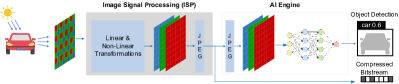
(a) Traditional RGB-Vision pipeline

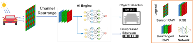
(b) The proposed $\rho$-Vision framework

Figure 1: Cameras for visual computing tasks. (a) Traditional RGB-Vision framework (with in-camera ISP) executes tasks with RGB images; (b) Proposed $\rho$-Vision framework (without conventional ISP) executes with RAW images directly.

The camera sensor and image signal processor (ISP) are tightly coupled for traditional RGB-Vision, as illustrated in Fig. 1a. First, a CMOS or CCD sensor records color pixels in a Bayer pattern as a RAW image. Then, an ISP converts the RAW image to RGB representation through a series of linear and nonlinear steps (e.g., demosaicing, white balance, exposure control, gamma correction, and JPEG compression) [7]. The compressed RGB images are then processed for various vision tasks and potentially stored for archival or review purposes.

The classic RGB-Vision pipeline used in cameras for decades has significant redundancies. As for the surveillance video usage reported by leading video hosting firms, less than $1\text{\,}\mathrm{\char 37\relax}$ of recorded videos are reviewed by human subjects [8]. The transformation process of the ISP is not just resource-intensive with additional hundreds of mW power consumption [9]—but also introduces additional processing delays. These delays are particularly detrimental in latency-sensitive applications, such as autonomous vehicles. Moreover, domain discrepancy is inevitable if we train and test models using RGB images generated from different ISPs, adversely affecting the inference accuracy. This raises a question why do we need the ISP to convert RAW images to the human-perceivable RGB format?

In this work, we present a $\rho$-Vision framework to execute both high-level and low-level tasks directly on camera RAW images. The key steps of $\rho$-Vision pipeline are illustrated in Fig. 1b. As an increasing number of artificial intelligence (AI) chips are installed on cameras [10], it is feasible to utilize in-camera AI chips for RAW image processing in various tasks.

One fundamental challenge in developing models for RAW-domain visual computing is the lack sufficient RAW images and task-associated label annotations to train robust RAW-domain models, since existing models are mainly developed for the RGB domain, large-scale, publicly accessible datasets consisting of RGB images (e.g., ImageNet [11]). On the other hand, directly applying pre-trained RGB-domain models to RAW images can lead to catastrophic performance degradation (see Table II).

To address the challenges posed by dataset limitations, we developed the Unpaired CycleR2R model. This model leverages existing RGB images to generate simulated RAW (simRAW) images. These simRAW images are produced using inverse ISP (invISP) methods, with which fine-tuning the existing RGB-domain models for RAW-domain tasks with uncompromised performance is assured. Training the Unpaired CycleR2R does not require paired RGB and RAW images. Instead, we can use the existing large-scale RGB dataset (e.g., 100,000 samples) and a much smaller RAW dataset (e.g., 7,000 images) to fulfill the purpose. This is particularly valuable given the challenges and high costs of acquiring a large-scale RAW image dataset (samples and label annotations). The Unpaired CycleR2R not only transforms the existing RGB dataset to its RAW-domain counterpart but also allows us to reuse its labels for subsequent task models directly, completely avoiding the tedious and expensive labeling. We then run a RAW-domain YOLOv3 to process RAW images, reporting better detection accuracy than the corresponding RGB-domain YOLOv3 used in several applications [12]. We also extend a variational autoencoder (VAE) based lossy/lossless RAW Image Compressor (RIC) from the TinyLIC [13] for RAW image compression. The resulting model shows superior performance to commercial approaches in both lossy and lossless modes.

This paper makes the following contributions:

1. Unpaired CycleR2R for conversion between RAW and RGB images. We train a CycleGAN to train an ISP for RAW-to-RGB and an invISP for RGB-to-RAW transformation (R2R) using unpaired RGB and RAW images. Unsupervised learning using unpaired samples makes our approach much more accessible for practical implementation. In contrast, existing solutions (e.g., CycleISP [14], CIE-XYZ Net [15], and MBISPLD [16]) are supervised models that require paired RAW and RGB images (from the same camera model).

   • Instead of training a generic deep network for ISP and invISP, we apply the modular unrolling to mimic functional steps in ISP and invISP subsystems, to which each step is motivated by imaging physics.

   • Since the same scene can be mapped into the different RAW samples by setting different brightness and color temperature levels, we characterize the probabilistic distribution of the illumination instead of using a fixed setting to best represent the practical conditions for the modeling of invISP/ISP.

2. RAW-domain models (in principle) can be obtained by retraining corresponding RGB-domain models using the simRAW images generated using the proposed invISP. Such domain adaptation approaches [17, 18, 19] need to be separately engineered for each individual task.

   • In our experiments, we demonstrate that YOLOv3 and RIC finetuned using simRAW samples provide outstanding performance for object detection and image compression in the RAW domain. We can consistently enhance their performance by further finetuning simRAW-tuned models with limited real RAW images from various camera models. Such a lightweight, few-shot fine-tuning method generalizes our method for camera-specific RAW-domain processing, which is attractive for practitioners.

   • To encourage the reproducible research, a labeled MultiRAW dataset that contains $>$7k RAW images acquired using multiple camera sensors is made publicly accessible for RAW-domain processing.

2 Related Work

This section briefly reviews relevant approaches for camera ISP, RAW image processing, and simRAW generation.

2.1 Camera ISP

Modern ISP converts sensor RAW data to RGB images using a series of computations, as shown in Fig. 1a. First, linear transformations, including demosaicing, white balance estimation, brightness adjustment, and color correction, are applied to map native RAW input to an intermediate format conforming to the CIE 1931 XYZ color space [20]. Subsequently, a sequence of nonlinear transformations translates the image from XYZ to RGB color space. Typical nonlinear operations include gamma correction and local transformations (e.g., denoising, sharpening, local tone mapping). Then, a JPEG encoder is used to compress the RGB images for storage or transmission. The entire processing pipeline of such ISP subsystems is widely used in commodity cameras. A white paper on the ISP system can be found here [21]. To summarize, the ISP mainly converts sensor RAW samples to human-perceivable RGB images, which induces redundant computations, as discussed earlier.

2.2 RAW Image Processing

Although most image processing algorithms have been developed for RGB images, recent explorations on RAW images have revealed superior performance for various tasks (e.g., denoising, deblurring) [22, 14, 16]. For instance, Brooks et al. [23] applied the UPI, Zamir et al. [14] proposed a CycleISP, Conde et al. [16] developed a learned dictionary-based model to convert an RGB image to its RAW format for denoising.

One challenge with processing RAW images is their strong dependence on specific sensors and devices, which makes the aforementioned methods difficult to generalize to multiple sensors. Afifi et al. [15] suggested processing images in device-independent CIE XYZ format that could be easily mapped from the sensor-specific RAW image via a colorimetric conversion. They not only reported performance improvement for various low-level tasks (e.g., denoising, deblurring, and defocusing) but also demonstrated the model generalization without requiring per-sensor supervision.

Existing works mainly focus on the low-level processing of RAW images. In this paper, we explore high-level semantic understanding tasks (e.g., object detection and segmentation). We also investigate low-level RAW image compression (RIC) for two reasons: 1) RIC is a commodity feature vastly used in cameras to ensure efficient storage and exchange of image snapshots; 2) the studies of denoising and deblurring in [15, 14, 16, 23] can be easily extended in our framework. To the best of our knowledge, this work, together with our earlier work in [24] offers the first study on the lossy and lossless compression of RAW images.

2.3 simRAW Generation

RAW-domain visual computing has promising prospects, as demonstrated by existing work, but training large neural networks for RAW-Vision requires large annotated datasets with RAW images. Collecting RAW images is somewhat easy and straightforward. However, the associated annotation labeling in the RAW domain is expensive and burdensome. Also, when we refer to a dataset used for the vision task, we generally assume the composite of the image samples and their label annotations. Thus, one approach is to generate RAW images from prevalent labeled RGB datasets, which requires reverse engineering the ISP, which we call invISP. Earlier algorithms, such as InvGamma [25], assume the availability of spectral characterization of a target camera to train the reverse imaging pipeline. Recently, CycleISP [14] and CIE-XYZ Net [15] suggested learning invISP module by fully leveraging the nonlinear representative capacity of underlying deep neural networks (DNNs). Training such models requires a large number of paired RAW and RGB images (e.g., DND dataset used by CycleISP [26] and MIT-Adobe FiveK [27] used in CIE-XYZ Net).

DNNs trained to characterize invISP (and ISP, if applicable) are hardly interpretable. Brooks et al. [23] (UPI) and Conde et al. [16] (MBISPLD) applied algorithm unrolling [28] to model modular components in the ISP subsystem by leveraging imaging physics. Such modular unrolling-based approaches were expected to require a small number of sample pairs for training [16]. Yet, UPI and MBISPLD still need paired RGB and RAW images, which limits the application in converting existing RGB datasets captured by unknown cameras, like BDD100K [29] into RAW format.

We propose the “Unpaired CycleR2R” to properly model the invISP and ISP functions. We not only follow the CycleGAN structure [17] to characterize the mapping functions using unpaired RAW (instantaneously captured by cameras) and RGB (obtained from existing datasets) images in an unsupervised manner but also enforce the modular unrolling approach for more robust model derivation. Though our method shares the general architecture of modular unrolling for invISP/ISP modeling with state-of-the-art MBISPLD [16], our method suggests the use of a probabilistic model to reflect non-bijective functional mapping in ISP modules. This is because the same RGB may come from a variety of RAWs acquired using different sensors or the same sensor with different illumination settings, while MBISPLD [16] strictly assumes the bijective mapping in the ISP subsystem.

3 Unpaired CycleR2R

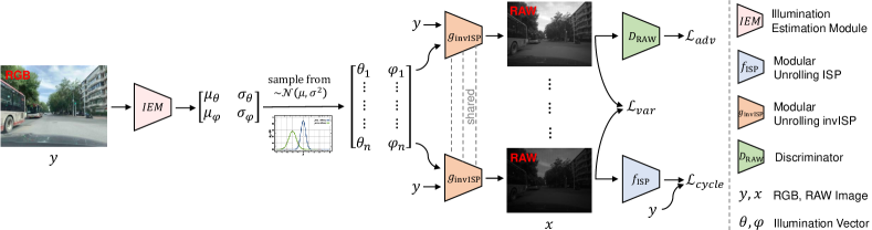
(a) Unpaired CycleR2R Framework.

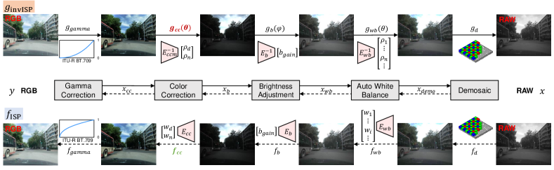
(b) Detail architectures of $g_{\rm invISP}$ and $f_{\rm ISP}$ .

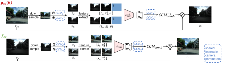
(c) Color correction $f_{cc}$ and inverse $g_{cc}(\theta)$.

Figure 2: Unpaired CycleR2R. (a) Our framework consists of an illumination estimation module (IEM) (Sec. 3.2), modular unrolling based ISP/invISP (Sec. 3.3) and unsupervised loss functions (Sec. 3.4). (b) The proposed framework simultaneously learns $g_{\rm invISP}$: RGB $\rightarrow$ RAW, and $f_{\rm ISP}$: RAW to $\rightarrow$ RGB with modular unrolling to best leverages the imaging physics in ISP/invISP for more robust model derivation. (c) Color correction $f_{cc}$ in $f_{\textrm{ISP}}$ and its inverse process $g_{cc}(\theta)$ in $g_{\textrm{invISP}}$ are exemplified while other modules mostly follow the similar method.

This section presents details on how to easily simulate realistic RAW (simRAW) images from existing RGB image datasets.

3.1 Problem Definition and CycleGAN Approach

Existing work in [14, 30, 15] model the invISP process from RGB to RAW ($g:\mathcal{Y}\rightarrow\mathcal{X}$) as a one-to-one mapping in a supervised manner, for which a large number of paired RAW and RGB images (from the same camera) are required. Apparently, such a one-to-one mapping-based invISP does not reflect the imaging circumstances in practice. For example, the same scene may be acquired as two different RAW samples because of different illumination settings, but the resultant RGB image (after the ISP) would be the same because the camera ISP is capable of making a proper estimation of those settings for realistic rendering.

The proposed Unpaired CycleR2R learns a one-to-many mapping of invISP through the introduction of the iillumination estimation module (IEM) that provides a distribution of color temperature $\theta$ and brightness $\phi$. Note that the use of unpaired RAW and RGB images avoids the collection of paired samples, making the solution more attractive and generally applicable in vast scenarios. Figure 2a provides an overview of the proposed Unpaired CycleR2R. We first use the IEM to estimate the illumination distribution of a scene. Then we sample a variety of $\theta$ and $\phi$ to simulate different illumination conditions used in practice (Sec. 3.2). These $\theta$ and $\phi$ are then used to generate various simRAW samples for a given RGB input (Sec. 3.3). We use a set of loss functions to guide the generation of realistic simRAW images (Sec. 3.4).

3.2 Illumination Estimation Module (IEM)

The same scene may appear differently in the RAW domain if different color temperature $\theta$ and brightness level $\phi$ are used in the acquisition. The ISP module estimates the $\theta$ and $\phi$ to generate properly-exposed RGB images under standard color temperature (D65 standard [31]). This suggests the one-to-many mappings from RGB to RAW and unknown values of $\theta$ and $\phi$ used in the camera make the invISP an ill-posed problem.

To tackle the ill-posed problem, we propose the IEM to estimate the original $\theta$ and $\phi$. We assume that the $\theta$ and $\phi$ follow the Gaussian distributions as $\mathcal{N}(\mu_{\theta},~{}\sigma_{\theta})$ and $\mathcal{N}(\mu_{\phi},~{}\sigma_{\phi})$ [32]. The IEM consists of three convolutional layers and two linear layers (see details in the supplemental material). During the training phase, the $\theta$ and $\phi$ are randomly sampled from Gaussian distribution and estimated through the guidance of $\mathcal{L}_{adv}$, $\mathcal{L}_{var}$ and $\mathcal{L}_{cycle}$ jointly to best simulate the real-world illumination.

3.3 Modeling of the ISP (invISP) via Modular Unrolling

Although it is possible to build a black box neural network to represent the ISP/invISP functions, an interpretable network design is preferred for robust inference and wide generalization [16, 28]. Therefore, we use modular unrolling to mimic the imaging physics involved in ISP and to build efficient $f_{\rm ISP}$/$g_{\rm invISP}$ used in the Unpaired CycleR2R framework.

Modern ISP systems in cameras are generally comprised of five major steps from RAW input to corresponding RGB output, as shown in Fig. 2b: demosaicing $f_{d}$, auto white balance $f_{wb}$, brightness adjustment $f_{b}$, color correction $f_{cc}$, and gamma correction $f_{g}$. Thus the ISP function can be expressed as:

$$f_{\textrm{ISP}} =f_{g}\circ f_{cc}\circ f_{b}\circ f_{wb}\circ f_{d},$$ (1)

$$\boldsymbol{y} =f_{\textrm{ISP}}\circ\boldsymbol{x},$$ (2)

where $\boldsymbol{y}\in\mathcal{Y}$ denotes an RGB image, $\boldsymbol{x}\in\mathcal{X}$ denotes a RAW image, and $\circ$ denotes the function composition operation. The invISP mirrors each step with illumination prior $\theta,~{}\phi$ as

$$g_{\textrm{invISP}} =g_{d}\circ g_{wb}(\theta)\circ g_{b}(\phi)\circ g_{cc}(\theta)\circ g_{g},$$ (3)

$$\boldsymbol{x} =g_{\textrm{invISP}}\circ\boldsymbol{y},$$ (4)

where we assume $g=f^{-1}$, for simplicity.

3.3.1 Demosaicing

Color (RGB) pixels on an image sensor are typically arranged in a Bayer pattern, half green, one-quarter red, and one-quarter blue (also called RGGB). To obtain a full-resolution color image, various demosaicing algorithms [33] have been developed in the past. For simplicity, we bilinearly upsample same-color pixels in close proximity to obtain demosaiced image $\boldsymbol{x}_{demo}$. Similarly, in invISP, we reverse the process to mosaic $\boldsymbol{x}_{demo}$ for its RAW output as

$$\boldsymbol{x}_{demo}=f_{d}\circ\boldsymbol{x},\mbox{~{}~{}~{}}\boldsymbol{x}=g_{d}\circ\boldsymbol{x}_{demo}.$$ (5)

3.3.2 Auto White Balance (AWB)

Cameras apply the white balance to ensure color constancy, which requires accurate approximation of the color temperature. Practical solutions often achieve this by augmenting the digital gains in Red and Blue channels [34, 23]. For instance, various gain presets, $\{(R_{gain},B_{gain})\}$ = $\{(r_{1},~{}b_{1}),\ldots,(r_{N},b_{N})\}$, can be defined for specific color temperatures. These presets are linearly weighted for auto white balance (AWB) because ambient illumination in real-life scenarios often mixes radiance from different light sources as

$$(r_{gain},b_{gain}) =W\cdot\{(R_{gain},~{}B_{gain})\}^{T}$$

$$=(\sum_{i=1}^{N}w_{i}r_{i},~{}\sum_{i=1}^{N}w_{i}b_{i}),$$ (6)

where $W=\{w_{1},\ldots,w_{N}\}$ is the weighting vector, and $N$ is total number of gain presets. As seen, accurate AWB relies on the proper choice of the $w_{i}$, $r_{i}$ and $b_{i}$ in $f_{wb}$ to derive $[r_{gain},1,b_{gain}]$ which is then multiplied with every pixel in the R, G, and B channels.

In general, the AWB function $f_{wb}$ in ISP maps the demosaiced image $\boldsymbol{x}_{demo}$ into a white-balanced image $\boldsymbol{x}_{wb}$. Given that AWB adjusts the global appearance of the image, we downscale the native input $\boldsymbol{x}_{demo}$ to $\boldsymbol{x}^{\downarrow}_{demo}$ at a size of 128$\times$128$\times$3 for processing, with which we can significantly reduce the space and time complexity. Specifically,

• Starting with $\boldsymbol{x}^{\downarrow}_{demo}$, we generate a pre-AWB image $\hat{\boldsymbol{x}}_{wb_{i}}$ by multiplying every channel with a preset gain $[r_{i},1,b_{i}]$. In training, we randomly initialize $r_{i}$, and $b_{i}$ following  [23]. As suggested in [35, 36] for camera AWB or color correction, $\hat{\boldsymbol{x}}_{wb_{i}}$ is paired with $\hat{\boldsymbol{x}}^{2}_{wb_{i}}$ for learning.

• Then, we propose the $E_{wb}(\cdot)$ that shares the same architecture with IEM, but with one-channel output, to process $\{\hat{\boldsymbol{x}}_{wb_{i}},~{}\hat{\boldsymbol{x}}^{2}_{wb_{i}}\}$ for weight derivation as

  $$w_{i}=E_{wb}(\{\hat{\boldsymbol{x}}_{wb_{i}},~{}\hat{\boldsymbol{x}}^{2}_{wb_{i}}\}),$$ (7)

  and subsequently the final AWB gain as in (6).

• Finally, instead of multiplying the AWB gain with every pixel of $\boldsymbol{x}_{demo}$ directly, highlight-preserving transformation $S(\boldsymbol{x},~{}\texttt{scalingFactor})$ is applied to avoid highlight overflow [23] as

  $$\boldsymbol{x}_{wb}=f_{wb}\circ\boldsymbol{x}_{demo}=S(\boldsymbol{x}_{demo},~{}[r_{gain},1,b_{gain}]).$$ (8)

Correspondingly, for $g_{wb}$ in invISP, we reverse engineer the $f_{wb}$ to derive $[1/r_{gain},~{}1,~{}1/b_{gain}]$. As mentioned before, the original color temperature is unknown in $g_{wb}$. Therefore, we model the inverse weights $\{\rho_{1},\ldots,\rho_{N}\}$ using $E^{-1}_{wb}$ with the color temperature prior $\theta$ estimated by the IEM. Note that $E^{-1}_{wb}(\cdot)$ shares the same architecture with $E_{wb}(\cdot)$. The processing steps are as follows.

• Apply preset inverse gain on downscaled input $\boldsymbol{x}_{wb}^{\downarrow}$ as $\hat{\boldsymbol{x}}_{demo_{i}}=[1/r_{i},~{}1,~{}1/b_{i}]\cdot\boldsymbol{x}_{wb}^{\downarrow}$.

• Derive the weight and inverse AWB gain as

  $$\rho_{i} =E^{-1}_{wb}(\{\hat{\boldsymbol{x}}_{demo_{i}},~{}\hat{\boldsymbol{x}}^{2}_{demo_{i}},~{}\theta\}),$$ (9)

  and compute $(1/r_{gain},~{}1/b_{gain})=\sum_{i}\rho_{i}\cdot(1/r_{i},~{}1/b_{i})$.

• Generate $\boldsymbol{x}_{demo}$ as

  $$\boldsymbol{x}_{demo}=g_{wb}(\theta)\circ\boldsymbol{x}_{wb}=[\frac{1}{r_{gain}},1,\frac{1}{b_{gain}}]\cdot\boldsymbol{x}_{wb}.$$ (10)

Such derivations of $w_{i}$ and $\rho_{i}$ are also used in brightness adjustment and color correction to characterize the non-bijective mapping.

3.3.3 Brightness Adjustment (BA)

Existing ISPs usually adjust the brightness of overexposed or underexposed RAW images by enforcing range-limited global gain $b_{gain}$ to scale every pixel uniformly [37]. We use a neural network $E_{b}(\cdot)$, which shares the same architecture as $E_{wb}(\cdot)$, to derive $b_{gain}$. We use a downscale and grayscale version of $\boldsymbol{x}_{wb}$, denoted as $\boldsymbol{x}_{wb}^{\downarrow G}$, because brightness adjustment is a global operation that does not require full-resolution spatial and spectral details.

We compute $b_{gain}={\beta+\alpha\cdot\textrm{tanh}(E_{b}(\boldsymbol{x}_{wb}^{\downarrow G}))}$, in the range of $[\beta-\alpha,\beta+\alpha]$ with $\alpha$ = 0.3 and $\beta$ = 1, following the suggestions in [23]. Finally, we also apply highlight-preserving transformation $S(\cdot,~{}\cdot)$ used in  [23] to have $\boldsymbol{x}_{b}$:

$$\boldsymbol{x}_{b}=f_{b}\circ\boldsymbol{x}_{wb}=S(\boldsymbol{x}_{wb},b_{gain}).$$ (11)

For $g_{b}$ in invISP, we reverse the adjustment on well-exposed $\boldsymbol{x}_{b}$ using $1/b_{gain}$. Considering that a series of images captured in the same scene using different exposure levels could be rectified to the same well-exposed image after brightness adjustment, we introduce the brightness prior $\phi$ to recover $\boldsymbol{x}_{wb}$ as

$$b_{gain}=\beta+\alpha\cdot\textrm{tanh}(E^{-1}_{b}(\{\boldsymbol{x}_{b}^{\downarrow G},\phi\})).$$ (12)

We multiply $1/b_{gain}$ with $\boldsymbol{x}_{b}$ to generate $\boldsymbol{x}_{wb}$ as

$$\boldsymbol{x}_{wb}=g_{b}\circ\boldsymbol{x}_{b}=1/b_{gain}\cdot\boldsymbol{x}_{b}.$$ (13)

3.3.4 Color Correction (CC)

In practice, a $3\times 3$ color correction matrix (CCM) is used in camera ISPs to restore the colors of the acquired image to match the human perception [15]. Similar to the AWB, camera vendors usually preset $\textrm{CCM}_{d}$ and $\textrm{CCM}_{n}$ for daytime and nighttime conversion, respectively [38]. The final transformation $f_{cc}$ is often derived by linearly combining the presets as

$$\textrm{CCM}_{mix}=\omega_{d}\cdot\textrm{CCM}_{d}+\omega_{n}\cdot\textrm{CCM}_{n}.$$ (14)

As shown in Fig. 2c, this work relies on a neural network $E_{cc}(\cdot)$ to produce respective $\omega_{d}$ and $\omega_{n}$. We compute $\omega_{d}$ as

$$\omega_{d}=E_{cc}(\{\hat{\boldsymbol{x}}_{d},~{}\hat{\boldsymbol{x}}^{2}_{d}\}),$$ (15)

where $\hat{\boldsymbol{x}}_{d}$ is computed by multiplying daytime CCM preset with every color pixel in the down-sampled $\boldsymbol{x}_{b}^{\downarrow}$ of size $128\times 128\times 3$ as $\hat{\boldsymbol{x}}_{d}=\textrm{CCM}_{d}\cdot\boldsymbol{x}_{b}^{\downarrow}$. The same procedure is applied to generate $\hat{\boldsymbol{x}}_{n}$, $\hat{\boldsymbol{x}}_{n}^{2}$ and compute $\omega_{n}$. During the training process, both $\textrm{CCM}_{d}$ and $\textrm{CCM}_{n}$ are randomly initialized following the same setting defined for $r_{i}$ and $b_{i}$ in $f_{wb}$.

Then (14) is used to compute the $\textrm{CCM}_{mix}$ as

$$\boldsymbol{x}_{cc}=f_{cc}\circ\boldsymbol{x}_{b}=\textrm{CCM}_{mix}\cdot\boldsymbol{x}_{b}.$$ (16)

The same $\boldsymbol{x}_{cc}$ may be produced by different $\boldsymbol{x}_{b}$ and different CCM scaling. Thus, following the discussions for $g_{wb}$, we use $E_{cc}^{-1}(\cdot)$ with color temperature prior $\theta$ to derive inverse weights $\rho_{d}$ and $\rho_{n}$ of $g_{cc}$, as $\rho_{d}=E^{-1}_{cc}(\{\hat{\boldsymbol{x}}_{d},~{}\hat{\boldsymbol{x}}_{d}^{2},~{}\theta\})$ and $\rho_{n}=E^{-1}_{cc}(\{\hat{\boldsymbol{x}}_{n},\hat{\boldsymbol{x}}_{n}^{2},~{}\theta\})$. Thereafter we can easily obtain $\textrm{CCM}_{mix}^{-1}$ as

$$\textrm{CCM}_{mix}^{-1}=(\rho_{d}\cdot\textrm{CCM}_{d}+\rho_{n}\cdot\textrm{CCM}_{n})^{-1}.$$ (17)

Finally, we have

$$\boldsymbol{x}_{b}=g_{cc}\circ\boldsymbol{x}_{cc}=\textrm{CCM}_{mix}^{-1}\cdot\boldsymbol{x}_{cc}.$$ (18)

3.3.5 Gamma Correction

Gamma correction is used to match the non-linear characteristics of a display device or human perception [39]. We adopt the correction function recommended in ITU-R BT. 709 standard [40], noted as $f_{g}$, which is widely used in commodity ISPs today [41]. Additional details are provided in the supplementary material.

3.4 Training Loss

We use three loss functions, denoted as $\mathcal{L}_{adv}$, $\mathcal{L}_{cycle}$ and $\mathcal{L}_{var}$, to train the Unpaired CycleR2R. The overall loss used to train our Unpaired CycleR2R can be written as

$$\mathcal{L}=\mathcal{L}_{adv}+\mathcal{L}_{cycle}+\mathcal{L}_{var}.$$ (19)

First, a discriminator $D_{\textrm{RAW}}$ is applied to measure the similarity between generated and real images. The discriminator can be further decomposed as $D_{\textrm{color}}$ and $D_{\textrm{bright}}$, where $D_{\textrm{color}}$ discriminates color discrepancy using 2D log-chroma histogram [42] and $D_{\textrm{bright}}$ discriminates brightness discrepancy using 1D grayscale histogram. $D_{\textrm{color}}$ stacks five convolutional layers with Leaky ReLU [43] and $D_{\textrm{bright}}$ uses five linear layers. The outputs of $D_{\textrm{color}}$ and $D_{\textrm{bright}}$ are added together as the output of $D_{\textrm{RAW}}$. We update the parameters of $g_{\textrm{invISP}}$ and $D_{\textrm{RAW}}$ by minimizing the adversarial loss $\mathcal{L}_{adv}$ given as

$$\mathcal{L}^{G}_{adv} =\|1-D_{\textrm{RAW}}(g_{\textrm{invISP}}({\boldsymbol{y}}))\|_{2},$$ (20)

$$\mathcal{L}^{D}_{adv} =\|1-D_{\textrm{RAW}}({\boldsymbol{x}})\|_{2}+\|D_{\textrm{RAW}}(g_{\rm invISP}({\boldsymbol{y}}))\|_{2},$$ (21)

$$\mathcal{L}_{adv} =\mathcal{L}^{G}_{adv}+\mathcal{L}^{D}_{adv}.$$ (22)

A cycle-consistency loss $\mathcal{L}_{cycle}$ is used to indirectly optimize $\theta$ and $\phi$ considering the assumption that RAW images captured under all possible illumination settings of the scene shall be converted into the same RGB sample. Thus the reconstructed RGB from the simRAW, given as $\overline{\boldsymbol{y}}=f_{\rm ISP}\circ g_{\rm invISP}\circ\boldsymbol{y}$, should be as close to the original RGB as possible, which gives us the following loss:

$$\mathcal{L}_{cycle}=\|\overline{\boldsymbol{y}}-\boldsymbol{y}\|_{1}.$$ (23)

The cycle-consistency constraint often leads to the one-to-one mapping of $g_{\rm invISP}$ in optimization [44]. To assure the one-to-many mapping of $g_{\rm invISP}$ in practice, another variant loss $\mathcal{L}_{var}$ is used with which we wish to enlarge the distance between two simRAW images $\boldsymbol{x}_{1}$ and $\boldsymbol{x}_{2}$ under two different illumination settings: $(\theta_{1},~{}\phi_{1})$ and $(\theta_{2},~{}\phi_{2})$. To independently evaluate the distance of color and brightness attributes, we measure the loss $\mathcal{L}_{var}$ in YUV space ($\boldsymbol{x}_{1}\rightarrow\{\textrm{y}_{1},~{}\textrm{u}_{1},~{}\textrm{v}_{1}\}$, $\boldsymbol{x}_{2}\rightarrow\{\textrm{y}_{2},~{}\textrm{u}_{2},~{}\textrm{v}_{2}\}$) as

$$\mathcal{L}_{var} =-\frac{\|\{\textrm{u}_{1},\textrm{v}_{1}\}-\{\textrm{u}_{2},\textrm{v}_{2}\}\|_{2}}{\|\theta_{1}-\theta_{2}\|_{2}}-\frac{\|\textrm{y}_{1}-\textrm{y}_{2}\|_{2}}{\|\phi_{1}-\phi_{2}\|_{2}}.$$ (24)

4 RAW-domain Task Execution

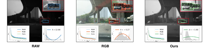
(a) The impact on Conv layer.

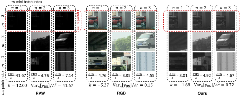
(b) The impact on BN layer.

Figure 3: Distribution impact of samples in native RAW, RGB, and Gamma-corrected (Ours) spaces. YOLOv3 is refined specifically for each domain space to quantify the distribution impact. (a) The fitted histogram distribution using (25) is shown in the lower right corner, where the RAW image has the largest value of $k$. As can be seen from the training loss plotted in the lower left corner, the convergence speed of the RAW image is the slowest, leading to the missing of critical objects during detection; (b) The variance of features across mini-batches with the same input patch is negatively correlated to the convergence of a neural network [45]. For the investigation of feature variance after a BN layer, ${\textrm{Var}}\,_{n}[\boldsymbol{y}_{\tt BN}]$, patches with index $m$ from mini-batches with index $n$ are randomly sampled in each domain. As seen, a large $k$ also leads to imbalanced variance across mini-batches, causing an unstable training process. The $\boldsymbol{y}_{\tt BN}$ is calculated using (31)

The generated simRAW images can be used to train RAW-domain models for various tasks. We discuss high-level object detection and low-level image compression tasks, for which we refine well-known models originally developed for RGB images.

4.1 High-Level Object Detection

Object detectors [12, 46, 47, 48, 49] have achieved great success in detecting objects in RGB images. The performance of off-the-shelf RGB-domain models such as YOLOv3 Fig. 3a presents an example where object is not detected on RAW image. The “Naive Baseline” in Table II, V also show a sharp loss in performance. This is counter-intuitive because sensor RAW data with a larger dynamic range shall contain more information on the physical scene than its ISP-processed RGB sample.

We argue that the vastly diverse distribution of RAW images significantly undermines the representation capacity of DNNs originally trained using RGB samples. We first use analytical approximation to show the impact of RAW data distribution on both convolution (Conv) and batch normalization (BN) layers commonly adopted in learned detectors [12, 50]; and then apply the gamma correction to regularize RAW image distribution for RAW-domain task inference.

4.1.1 Distribution Analysis of RAW Images

Distribution approximation using patches. In practice, an input image $\boldsymbol{x}$ is often divided into non-overlapping small patches $\mathcal{P}=\{\boldsymbol{P}_{1},\boldsymbol{P}_{2},\ldots\}$ to train desired models for task inference [12, 51]. For a patch $\boldsymbol{P}\in\mathcal{P}$, its histogram can be approximated using a Gaussian distribution $\mathcal{N}(\mu,~{}\sigma^{2})$. To simplify modeling the distribution of pixel intensity $p(\mathbf{x})$ over the entire image using patches, we treat each patch $\boldsymbol{P}$ as a superpixel with intensity $\mu$ and assume that the $p(\mathbf{x})$ can be approximated by $p(\mu)$.

Referring to the RAW snapshot depicted in the leftmost subplot of Fig. 3a, most pixel patches are clustered in dark and bright regions, which yield histogram peaks near 0 and 1. Therefore, $p(\mu)$ can be possibly hypothesized using a U-shaped function. In the meantime, without losing generality for image with proper exposure control, the mean of the entire image shall be close to the middle level of the dynamic range, which, in other words, for normalized RAW image, $\mathbb{E}[p(\mu)]$ = 0.5. It then leads us to approximate $p(\mu)$ using a quadratic function:

$$p(\mathbf{x})\approx p(\mu)\approx k\mu^{2}-k\mu+\frac{k}{6}+1,$$ (25)

with $0<k\leq 12$ to guarantee $\min\{p(\mu)\}\geq 0$. Coincidentally, (25) also models the histogram of normalized RGB image very well but has the $k<0$. As seen, $k$ can be used to characterize the distribution of the input image (RAW or RGB). We next show that $k$ impacts the performance of Conv and BN layers analytically, which in turn, explains why native YOLOv3 trained for RGB images cannot be directly used to process RAW samples.

Effect of $k$ on convergence. Suppose $\boldsymbol{w}\in\mathbb{R}^{S\times S}$ denotes the Conv kernel weights randomly initialized with $\mathcal{U}(-\eta,~{}\eta),~{}\eta\to 0$, and $\mathbf{b}$ is the Conv bias that is randomly initialized in same manner as the weights. Then a single layer of CNN can be represented as

$$\boldsymbol{y}=\boldsymbol{w}\ast\tilde{\boldsymbol{x}}+\mathbf{b},$$ (26)

where $\tilde{\boldsymbol{x}}=\boldsymbol{x}-0.5$ shifts the center to zero. As for the bounding box regression of the input patch $\boldsymbol{P}\sim\mathcal{N}(\mu,\sigma^{2})$ in YOLOv3 [12], the loss function $\mathcal{L}$ is

$$\mathcal{L}=\frac{1}{H\times W}(\boldsymbol{w}\ast(\boldsymbol{P}-0.5)+\mathbf{b}-\hat{\mathbf{y}})^{2},$$ (27)

having $\hat{\mathbf{y}}$ as the ground truth label, and $H$/$W$ as the height/width of $\boldsymbol{P}$.

For each training iteration, the weight $w\in\boldsymbol{w}$ is updated with learning rate $\alpha$, i.e., $w\leftarrow w-\alpha\frac{\partial\mathcal{L}}{\partial w}.$ The stability of parameter update is directly related to the variance of the gradient ${\textrm{Var}}\,[\frac{\partial\mathcal{L}}{\partial w}]$ as shown in [50]. This variance is approximately given as

$${\textrm{Var}}\,[\frac{\partial\mathcal{L}}{\partial w}] \approx C^{2}{\textrm{Var}}\,[\tilde{\mu}^{2}]+D^{2}{\textrm{Var}}\,[\tilde{\mu}]+\textrm{const},$$ (28)

where $\tilde{\mu}=\mu-0.5$, $C=2\sum w=2S^{2}\mathbb{E}[w]$, and $D$ is a constant. Since $w$ is randomly initialized with a small value close to zero, $\mathbb{E}[w]\approx 0$, which simplifies (28) to:

$$\begin{split}{\textrm{Var}}\,[\frac{\partial\mathcal{L}}{\partial w}]&\approx D^{2}{\textrm{Var}}\,[\tilde{\mu}]+\textrm{const}=\frac{D^{2}}{180}k+\textrm{const}.\end{split}$$ (29)

This shows that the variance of the gradient is directly related to the parameter $k$. A larger $k$ provides larger ${\textrm{Var}}\,[\frac{\partial\mathcal{L}}{\partial w}]$, making the convergence of the Conv weights more difficult and the CNN model unreliable. The proofs of (28) and (29) are provided in the Supplemental Material.

Effect of $k$ on batch normalization.

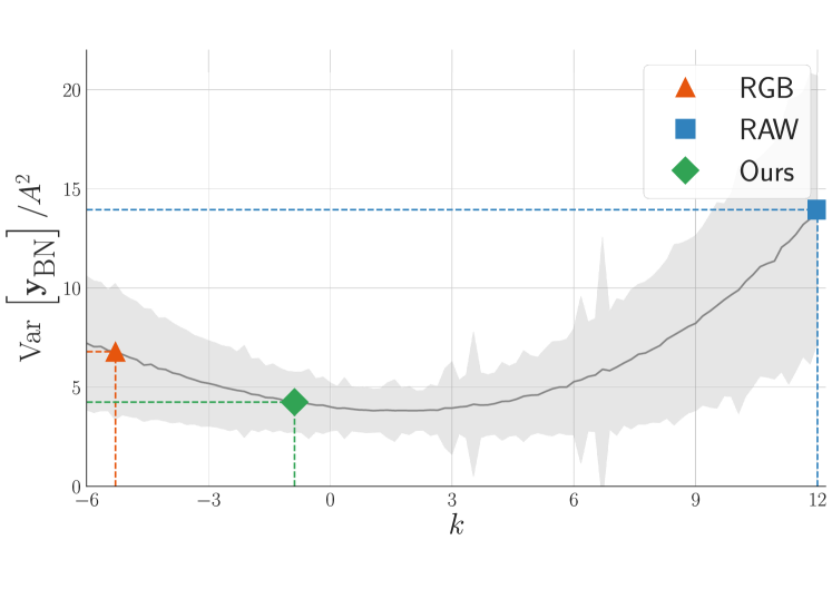
Figure 4: ${\textrm{Var}}\,_{n}\left[\boldsymbol{y}_{\tt{BN}}\right]/A^{2}$ vs. $k$.

Batch Normalization [52] (BN) randomly splits a batch of training samples into mini-batches during training iteration to assure stability. A BN layer is usually placed after a convolutional layer in order to normalize the output features. Given an input patch with index $m$ from a mini-batch with index $n$ of size $M$, the output of the BN layer is given by:

$$\boldsymbol{y}_{\tt BN}=\textrm{BN}(\boldsymbol{y}^{\ell mn})=\gamma\frac{\boldsymbol{y}^{\ell mn}-\mathbb{E}_{m}[\boldsymbol{y}^{\ell mn}]}{\sqrt{{\textrm{Var}}\,_{m}[\boldsymbol{y}^{\ell mn}]}}+\beta,$$ (30)

where $\gamma$ and $\beta$ are learnable parameters, and $\boldsymbol{y}^{\ell mn}$ is the feature of layer $\ell$.

It is vital for the convergence of a neural network that the mean and variance of features with the same input patch are similar across mini-batches during training [45]. Thus, we can measure the convergence speed of a model by the cross-batch variance ${\textrm{Var}}\,_{n}[\boldsymbol{y}_{\tt BN}]$. The larger ${\textrm{Var}}\,_{n}[\boldsymbol{y}_{\tt BN}]$ leads to the imbalance among mini-batches and thus yields an unstable training gradient. In the following part, we will demonstrate that ${\textrm{Var}}\,_{n}[\boldsymbol{y}_{\tt BN}]$ increases significantly for RAW images having larger $k$, which degrades the training stability of the RAW-domain detector.

We will start by modeling the relationship between the input patch $\boldsymbol{P}^{mn}$ and $\boldsymbol{y}_{\tt BN}$. As proven in [53], we have that $\mathbb{E}_{m}[\boldsymbol{y}^{\ell mn}]$ is approximately 0 and its variance is approximately $\alpha_{l}\cdot{\textrm{Var}}\,_{m}[\boldsymbol{y}^{\ell-1mn}]$, where $\alpha_{l}$ is a constant when the weight of layer $l$ is fixed. Therefore, the relationship can be recursively derived as follows:

$$\boldsymbol{y}_{\tt BN}\approx\frac{A}{\sqrt{{\textrm{Var}}\,_{m}[\boldsymbol{P}^{mn}-0.5]}}+\beta,$$ (31)

where $A=\gamma\cdot\boldsymbol{y}^{\ell mn}/\prod_{i=1}^{\ell}\sqrt{\alpha_{i}}$ is a constant when the input patch $\boldsymbol{P}^{mn}$ is fixed.

Next, we will model the variance ${\textrm{Var}}\,_{n}[\boldsymbol{y}_{\tt{BN}}]$ across mini-batches. Given  (31), we simplify the variance as:

$${\textrm{Var}}\,_{n}[\boldsymbol{y}_{\tt BN}]\approx A^{2}\cdot\mathop{{\textrm{Var}}\,}_{n}[\frac{1}{\sqrt{\mathop{{\textrm{Var}}\,}_{m}[\boldsymbol{P}^{mn}-0.5]}}].$$ (32)

Due to the limited batch size $M$, it is difficult to obtain a closed-form probability distribution of $\boldsymbol{P}^{mn}$. Therefore, we resort to sampling simulations for approximation. To simplify the problem, we neglect the variance in a patch and represent it with its mean value $\mu$. We obtain the value of ${\textrm{Var}}\,_{n}[\boldsymbol{y}_{\tt BN}]/A^{2}$ using $5000$ randomly-sampled mini-batches that contain the same patch $\boldsymbol{P}^{mn}$ characterized by $p(\mu)$ in (25). The whole process is repeated $5000$ times using different randomly-sampled $\boldsymbol{P}^{mn}$ to obtain the average value of ${\textrm{Var}}\,_{n}[\boldsymbol{y}_{\tt{BN}}]/A^{2}$. Figure 4 shows the quantitative approximation between ${\textrm{Var}}\,_{n}[\boldsymbol{y}_{\tt{BN}}]/A^{2}$ and $k$. It is clear that ${\textrm{Var}}\,_{n}[\boldsymbol{y}_{\tt BN}]$ increases significantly for larger values of $k$.

Remark. As seen, larger $k$ induced by the RAW input slows the convergence of convolutional weights and yields unstable batch normalization, making the underlying model unreliable and inefficient, which requires us to regularize the distribution of RAW images for robust performance.

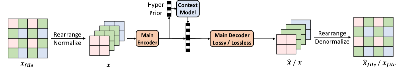
(a) RAW Image Compression (RIC) Architecture

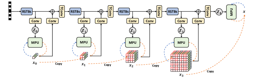
(b) Lossless RIC Decoder

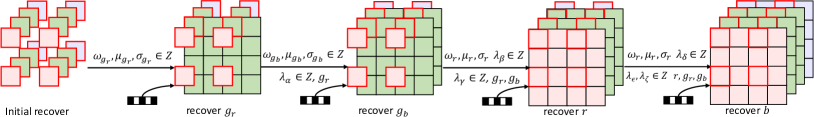
(c) Multichannel Processing Unit (MPU)

Figure 5: RAW Image Compression (RIC). (a) Similar TinyLIC architectures are used for both lossy and lossless RIC. More details about the lossy pipeline are in [13]. (b) The detailed architecture of the lossless decoder. $\boldsymbol{Z}_{i}$, $i\in[0,4]$ aggregates low-resolution information to characterize the logistic distribution for element probability derivation. The probability is used for both encoding (blue) and decoding (orange). In decoding, $\boldsymbol{x}$ are gradually recovered with progressive decoding; (c) Multichannel Processing Unit (MPU) is devised to process the element in $\boldsymbol{x}_{i}$ with the probability derived from the $\boldsymbol{Z}_{i}$ under a predefined order, e.g., $g_{r}\rightarrow g_{b}\rightarrow r\rightarrow b$. Arithmetic decoding is omitted. Residual Swin Transformer Blocks (RSTBs) are stacked to aggregate and embed necessary information. The Conv and TConv stand for the convolutional and transposed convolutional layer respectively.

4.1.2 Distribution Regularization Using Gamma Correction

To eliminate the negative impact of a large $k$ of a RAW image for RAW-domain detection, we use a simple-yet-efficient gamma correction defined in ITU-R BT.709 [40] to reduce the $k$ by brightening the dark area and darkening the light area. As shown in the rightmost subplot of Fig. 3, those sub-images generated by the gamma correction effectively reduce the $k$ of the original RAW input, making the convergence of RAW-domain detector faster and the resultant model more robust with better performance (see Table V).

4.2 Low-Level RAW Image Compression

Applications often mandate the archival of images for after-action review and analysis, leading to the desire for high-efficiency image compression. Existing image codecs mainly deal with RGB, monochrome, or YCbCr color spaces. In this section, we explore the feasibility of encoding RAW images directly. We suggest using learned image compression for this purpose, not only because of its superior coding efficiency [54, 55, 13] but also its flexibility to support the coding of various image sources.

4.2.1 Lossy RAW Image Compression (RIC)

We extend the TinyLIC proposed in [13] for lossy RIC with the following amendments shown in Fig. 5a:

1. Rearrangement: First, we follow [56] to rearrange Bayer RAWs to RGGB presentation. At each pixel position, its spectral components, e.g., (R, G, G, B), are stacked for compression, which is similar to the pixel of (R, G, B) used in default TinyLIC;

2. Normalization: We normalize the original Bayer RAW files through linearization using

   $$\boldsymbol{x}=\frac{\boldsymbol{x}_{file}-\texttt{blackLev}}{\texttt{saturationLev}-\texttt{blackLev}},$$ (33)

   where $\boldsymbol{x}_{file}$ is the Bayer RAW collected by an image sensor, and $\boldsymbol{x}$ is normalized RAW in the range of [0, 1]. saturationLev and blackLev indicate the dynamic range of image pixels, which can be directly retrieved from the EXIF metadata of the RAW input.

The saturationLev is related to the bit depth supported by the specific camera for RAW acquisition. It is the same for all RAW images captured by the same camera. We choose to embed the blackLev coefficients globally (e.g., $1\times 16=16~{}\textrm{bits}$ present $<$ $0.03\text{\,}\mathrm{\char 37\relax}$ of the total bits used by a $512\times 512$ image) to ensure the encoder-decoder consistency. Stacking RGGB components could let the lossy RIC explicitly learn the inter-spectral or inter-color correlations. As will be shown later, our lossy RIC significantly outperforms the traditional methods on RAW encoding. For other imaging patterns, e.g., RYYB used in the Huawei P30 Pro can be processed similarly.

4.2.2 Lossless RIC

Numerous applications need to cache RAW images losslessly for future processing (e.g., professional photography, safety-critical event record, etc.). We further extend the lossy RIC to support the lossless mode.

Multiresolution Decoding. In lossy RIC, the processing steps in the main encoder-decoder pair are symmetrically mirrored [13]. In lossless RIC, we redesign the main decoder while keeping the same main encoder as in lossy RIC. Instead of decoding the full-resolution reconstruction in one shot, we gradually decode the pixels to refine the image resolution from $\boldsymbol{x}_{0}$ to $\boldsymbol{x}_{4}$ ($\boldsymbol{x}_{4}$ = $\boldsymbol{x}$) in Fig. 5b. As seen, the compression performance is improved by exploiting the correlations from previously-decoded neighbors. Such progressive decoding enables the low-resolution preview that is not available in existing approaches [57, 58] but is a highly-desired tool in commercial cameras.

The lossless decoding of $\boldsymbol{x}_{i}$, $i\in[1,4]$ is organized as:

1. The $\boldsymbol{x}_{i}$ is dyadically upsampled from $\boldsymbol{x}_{i-1}$ with 2$\times$ scaling at each dimension, i.e., each pixel in $\boldsymbol{x}_{i-1}$ is expanded to four pixels arranged in a local 2$\times$2 patch in $\boldsymbol{x}_{i}$;

2. As in Fig. 5b, the upper-left pixel of each 2$\times$2 patch of $\boldsymbol{x}_{i}$ is directly filled using the corresponding pixel of $\boldsymbol{x}_{i-1}$ (highlighted with red box), while the other three pixels in each 2$\times$2 patch of $\boldsymbol{x}_{i}$ is decoded using the conditional probability of logistic distribution that is characterized by the $\boldsymbol{Z}_{i}$;

Note that a special case is made for the processing of $\boldsymbol{x}_{0}$ since there are no available pixels from a lower resolution scale. As a result, $\boldsymbol{Z}_{0}$ is generated by parsing the compressed bitstream only.

Multichannel Processing. As seen, $\boldsymbol{Z}$ thoroughly aggregates information from the lower resolution scale, which is then input into the Multichannel Processing Unit (MPU) to encode/decode pixels in a predefined order to fully exploit the cross-channel correlations. Here, we use $r,g_{r},g_{b},b$ to represent four Bayer pattern channels. For the MPU in Fig 5c, only $\boldsymbol{Z}$ is used to derive the probability of $g_{r}$ samples for its encoding and decoding first. Then both $\boldsymbol{Z}_{i}$ and previously-processed samples are used to process $g_{b}$, $r$, and $b$ sequentially. Here we parameterize the sample distribution $P$ as a mixture of logistic distribution $P_{l}$ [59]:

$$\begin{split}P(g_{r}~{}|~{}\boldsymbol{Z})&=\sum\nolimits_{k=1}^{K}\omega_{g_{r}k}\cdot P_{l}(g_{r}~{}|~{}\mu_{g_{r}k},\sigma_{g_{r}k})\\ P(g_{b}~{}|~{}\boldsymbol{Z},g_{r})&=\sum\nolimits_{k=1}^{K}\omega_{g_{b}k}\cdot P_{l}(g_{b}~{}|~{}\tilde{\mu}_{g_{b}k},\sigma_{g_{b}k})\\ P(r~{}|~{}\boldsymbol{Z},g_{r},g_{b})&=\sum\nolimits_{k=1}^{K}\omega_{rk}\cdot P_{l}(r~{}|~{}\tilde{\mu}_{rk},\sigma_{rk})\\ P(b~{}|~{}\boldsymbol{Z},g_{r},g_{b},r)&=\sum\nolimits_{k=1}^{K}\omega_{bk}\cdot P_{l}(b~{}|~{}\tilde{\mu}_{bk},\sigma_{bk}),\\ \end{split}$$ (34)

where the $\tilde{\mu}$ builds the cross channels dependency:

$$\begin{split}\tilde{\mu}_{g_{b}k}&=\mu_{g_{r}k}+\lambda_{\alpha k}\cdot g_{r},\\ \tilde{\mu}_{rk}&=\mu_{rk}+\lambda_{\beta k}\cdot g_{r}+\lambda_{\gamma k}\cdot g_{b},\\ \tilde{\mu}_{bk}&=\mu_{bk}+\lambda_{\delta k}\cdot g_{r}+\lambda_{\epsilon k}\cdot g_{b}+\lambda_{\zeta k}\cdot r.\end{split}$$ (35)

The logistic function $P_{l}(x|\mu,\sigma)$ can be easily calculated using {$\textrm{sigmoid}(\frac{x-\mu+1/2s}{\sigma})$ - $\textrm{sigmoid}(\frac{x-\mu-1/2s}{\sigma})$} with $s$ = saturationLev-blackLev. Parameters $\mu,\sigma,\omega$ and $\lambda$ are a part of the prior $\boldsymbol{Z}$ and we set $K=10$ as in [60, 59]. In training, we only need to minimize the entropy loss $\mathcal{L}=-\mathbb{E}\left[\log P(r,g_{r},g_{b},b~{}|~{}\boldsymbol{Z})\right]$ for lossless compression.

5 Experimental Results

This section presents experiments where we execute tasks using RAW images directly.

TABLE I: MultiRAW Dataset: A collection of 7,469 labeled RAW images from five diverse camera sensors. The dataset covers various settings (e.g., Bayer pattern, bit depth) and application scenarios.

Camera	Usage	Bayer Pattern	Bit Depth	Task	Scenarios	No. of Images
iPhone XSmax	Mobile	RGGB	12	Detection, Segmentation	Day	1153
Huawei P30pro	Mobile	RYYB	12	Detection	Day, Night	3004
asi 294mcpro	Industrial	RGGB	14	Detection	Day, Night	2950
Oneplus 5t	Mobile	RGGB	10	Detection	Day	101
LUCID TRI054S	Autopilot	RGGB	24	Detection	Day, Tunnel	261

5.1 Experiment Setup

We first list the RAW and RGB image datasets used in experiments, and then discuss the setup of the proposed Unpaired CycleR2R to generate simRAW images.

TABLE II: Recall and Average Precision (AP) of Object Detection on the testing set of iPhone RAWs. RGB detector is trained using original RGB images in BDD100K [29] (e.g., $\text{RGB}_{\text{b}}$); Various simRAW datasets associated with $\text{RGB}_{\text{b}}$ are generated using different methods which are simply marked as sim$\text{RAW}_{\text{b}}$ to train the RAW detector. The testing RAW images in iPhone RAW $\text{RAW}_{\text{i}}$ and their paired RGB images in $\text{RGB}_{\text{i}}$ converted using built-in iPhone ISP are tested accordingly. All detectors are shared with the same head, i.e., YOLOv3 [12] and the same backbone, i.e., MobileNetV2 [61] for a fair comparison. $\spadesuit$ Baselines, $\blacklozenge$ Domain Adaptation Solutions, $\blacksquare$ invISP Methods, $\bigstar$ Ours.

Method	invISP Training	Detector Training	Detector Testing	Recall	AP
$\spadesuit$ Naive Baseline	-	$\text{RGB}_{\text{b}}$	$\text{RAW}_{\text{i}}$	67.5	51.1
$\spadesuit$ RGB Baseline	-	$\text{RGB}_{\text{b}}$	$\text{RGB}_{\text{i}}$	74.7	55.6
$\blacklozenge$ DA-Faster (CVPR’18) [62]	-	$\text{RGB}_{\text{b}}$, $\text{RAW}_{\text{i}}$	$\text{RAW}_{\text{i}}$	13.7	12.9
$\blacklozenge$ MS-DAYOLO (ICIP’21) [18]	-	$\text{RGB}_{\text{b}}$, $\text{RAW}_{\text{i}}$	$\text{RAW}_{\text{i}}$	31.2	29.7
$\blacklozenge$ AT (CVPR’22) [19]	-	$\text{RGB}_{\text{b}}$, $\text{RAW}_{\text{i}}$	$\text{RAW}_{\text{i}}$	68.9	53.2
$\blacksquare$ InvGamma (ICIP’19) [25]	$\text{RGB}_{\text{i}}$, $\text{RAW}_{\text{i}}$	sim$\text{RAW}_{\text{b}}$	$\text{RAW}_{\text{i}}$	68.6	48.7
$\blacksquare$ CycleISP (CVPR’20) [14]	$\text{RGB}_{\text{i}}$, $\text{RAW}_{\text{i}}$	sim$\text{RAW}_{\text{b}}$	$\text{RAW}_{\text{i}}$	71.6	52.7
$\blacksquare$ CIE-XYZ Net (TPAMI’21) [15]	$\text{RGB}_{\text{i}}$, $\text{RAW}_{\text{i}}$	sim$\text{RAW}_{\text{b}}$	$\text{RAW}_{\text{i}}$	72.2	53.0
$\blacksquare$ MBISPLD (AAAI’22) [16]	$\text{RGB}_{\text{i}}$, $\text{RAW}_{\text{i}}$	sim$\text{RAW}_{\text{b}}$	$\text{RAW}_{\text{i}}$	73.0	53.7
$\bigstar$ Unpaired CycleR2R	$\text{RGB}_{\text{b}}$, $\text{RAW}_{\text{i}}$	sim$\text{RAW}_{\text{b}}$	$\text{RAW}_{\text{i}}$	76.1	59.1

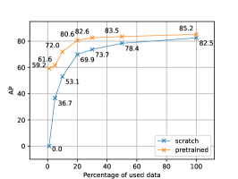
(a) iPhone XSmax.

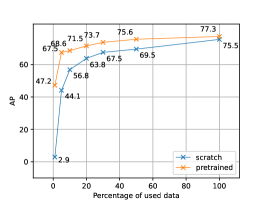
(b) Huawei P30pro.

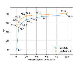
(c) asi 294mcpro.

Figure 6: Few-shot model finetuning using limited camera RAWs. The “pretrained” YOLOv3 is pretrained using samples in simRAW${}_{\text{b}}$ generated by our invISP, and the “scratch” model is first randomly initialized and then directly trained using labeled real RAW images from a specific camera model.

5.1.1 Datasets

MultiRAW is a high-resolution RAW image dataset acquired using popular camera sensors. Specifically, the entire dataset was shot using five cameras fixed on the car dashboard at different times (day and night) and geolocations (rural, tunnel, and urban areas) to simulate real-life autonomous driving. Having RAW images from different cameras allows us to validate the generalization of the proposed method.

Table I provides details about 7,469 RAW images that cover a variety of application scenarios (mobile/ industrial/autopilot), imaging Bayer patterns ( RGGB/RYYB), and bit depths (e.g., $10$/$12$/$16$/$24$). All RAW images could be converted to RGB counterparts using the corresponding in-camera ISP. Fine-grained detection and segmentation bounding boxes for cars, persons, traffic lights, and traffic signs are labeled manually by a third-party professional image labeling firm.

Among the RAW images captured by iPhone XSmax, Huawei P30pro, asi 294mcpro, and the LUCID TRI054S, we randomly selected $30\text{\,}\mathrm{\char 37\relax}$ samples as the test set and the remaining ones as the training set. For RAW images acquired by Oneplus 5t, we use all of them for testing.

BDD100K [29] is one of the largest autonomous driving datasets. It contains $100\text{\,}\mathrm{k}$ RGB images taken in diverse scenes such as city streets, residential areas, and highways, making object detection more challenging and close to real-life scenarios. We follow the official data splitting of $70\text{\,}\mathrm{k}$, $10\text{\,}\mathrm{k}$, and $20\text{\,}\mathrm{k}$ images for training, validation, and testing, respectively. To avoid the discrepancy of traffic signs captured in BDD100K (e.g., collected across tens of different countries) and MultiRAW (e.g., collected mainly in mainland China) datasets, we only conducted training and testing on the “car” category that has the largest number of objects (e.g., $>$$55\text{\,}\mathrm{\char 37\relax}$) and presents the smallest differences.

Flicker2W [63] is widely used to train learned image compressors [13]. Although we collected more than 7k samples in MultiRAW, its size is less than that of RGB image datasets (e.g., 100k in BDD100K) used in popular tasks. To train robust models, we apply our Unpaired CycleR2R to generate simRAW images using popular RGB datasets. For example, all RGB samples in BDD100K and Flickr2W are converted to RAW images to retrain existing RGB-domain models.

5.1.2 Training Unpaired CycleR2R for simRAW Generation

We first train our Unpaired CycleR2R to generate simRAW images to finetune/retrain existing RGB-domain models for RAW-domain tasks. For example, unpaired RGB and iPhone RAW images that were respectively chosen from the BDD100K [29] (without knowledge of camera sensors) and MultiRAW datasets are used to train the Unpaired CycleR2R for the high-level detector. We also use the original Flicker2W [63] along with the random iPhone RAW images to train the Unpaired CycleR2R for the low-level compressor.

We train the model using randomly selected patches of size $512\times 512$ and batch size $8$. We applied random scaling and reflection to augment the training data. A single NVIDIA 3090Ti was used for $20,000$ iterations of an Adam optimizer with a learning rate $5\cdot 10^{-4}$. The discriminators were set with a learning rate at $5\cdot 10^{-5}$. The momentum for Adam is set to $\left\{0.9,0.99\right\}$. Finally, $g_{\rm invISP}$ from the Unpaired CycleR2R framework was used to produce simRAW_b and simRAW_f images using RGB images in BDD100K [29] and Flicker2W [63].

5.2 RAW-domain Object Detection

This section shows that the object detector trained on simRAW images can directly process real-life RAW images and provide good accuracy. Then, we discuss how the performance of a simRAW-pretrained detector can be further improved by the few-shot finetuning using a limited number of labeled real RAW images from a camera used in a specific application scenario. Our results show that such a few-shot fine-tuned detector consistently outperforms the model trained from scratch using the same set of real RAW images.

Training RAW-domain detector. We chose the popular YOLOv3 as our baseline object detector [12] and the prevalent MobileNetv2 [61] as the backbone.

• RAW-domain YOLOv3 can be trained using simRAW_b set generated from the RGB samples (RGB_b) in BDD100K using various invISP methods [25, 14, 15, 16] (see Table II). We trained YOLOv3 using SGD with the batch size at $8$, a momentum of $0.9$, and a weight decay of $10^{-4}$. A learning rate of $0.02$ was used in training for $30$ epochs.

• RAW-domain YOLOv3 can also be retrained using unpaired RGB_b and RAW_i sets of respective BDD100K and iPhone RAW (a subset of MultiRAW) through the use of domain adaptation (DA) techniques following their official settings [62, 18, 19].

We tested the trained models on the test set of RAW_i.

Remark. For the invISP methods listed in Table II that strictly required RGB-RAW pairs from a specific camera model, we fine-tuned their pre-trained models using our MultiRAW dataset by applying the same training settings used to train our Unpaired Cycle R2R model (i.e. epochs, training patches).

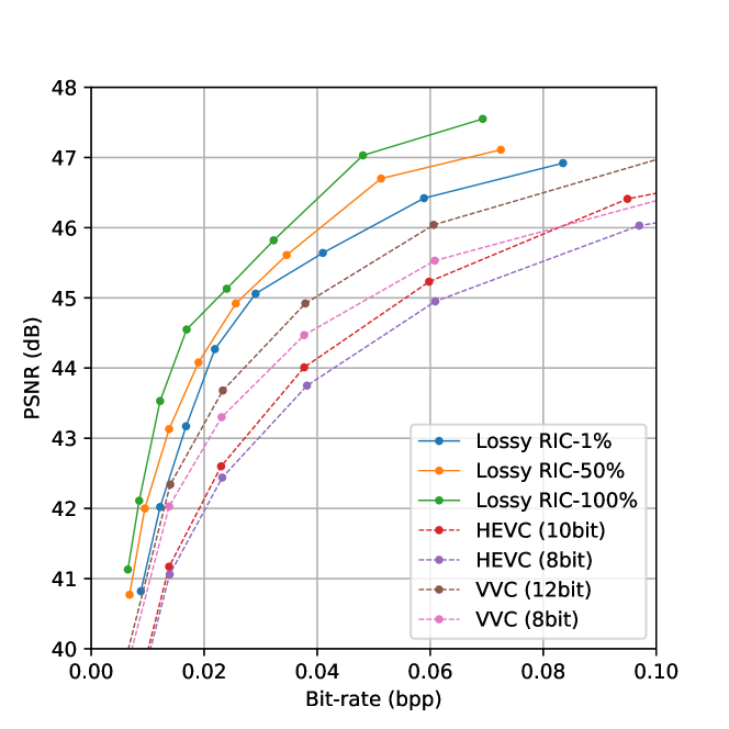
Figure 7: Rate-distortion Performance of Lossy RIC. These testing RAW images are from our MultiRAW dataset and distortion is measured in the RAW domain. All RICs are pre-trained with simRAW images and fine-tuned using a limited number of real captured RAWs. Lossy RIC-$1\text{\,}\mathrm{\char 37\relax}$, Lossy RIC-$50\text{\,}\mathrm{\char 37\relax}$ and Lossy RIC-$100\text{\,}\mathrm{\char 37\relax}$ denote $1\text{\,}\mathrm{\char 37\relax}$, $50\text{\,}\mathrm{\char 37\relax}$ and $100\text{\,}\mathrm{\char 37\relax}$ real RAW samples are used for fine-tuning. HEVC and VVC Intra coders are evaluated for comparison.

TABLE III: The lossless compression results on MultiRAW.

Method	Camera	Latency (s)		BPP
		Encoder	Decoder
CinemaDNG	iPhone XSmax (RGGB/$12\text{\,}\mathrm{b}\mathrm{i}\mathrm{t}\mathrm{s}$) $4032\times 3024$	0.49	0.52	9.51
JPEG XL		19.73	6.38	5.46
FLIF		38.67	8.76	5.46
PNG		0.44	0.24	7.98
Lossless RIC-$1\text{\,}\mathrm{\char 37\relax}$		1.35	0.78	5.29
Lossless RIC-$100\text{\,}\mathrm{\char 37\relax}$				5.21
CinemaDNG	Huawei P30pro (RYYB/$12\text{\,}\mathrm{b}\mathrm{i}\mathrm{t}\mathrm{s}$) $4032\times 3024$	0.42	0.46	9.52
JPEG XL		21.37	6.67	5.62
FLIF		41.67	9.56	5.60
PNG		0.39	0.22	7.93
Lossless RIC-$1\text{\,}\mathrm{\char 37\relax}$		1.32	0.79	5.16
Lossless RIC-$100\text{\,}\mathrm{\char 37\relax}$				5.12
CinemaDNG	asi 294mcpro (RGGB/$14\text{\,}\mathrm{b}\mathrm{i}\mathrm{t}\mathrm{s}$) $4144\times 2822$	0.40	0.44	18.85
JPEG XL		9.37	2.91	1.46
FLIF		18.83	4.26	1.36
PNG		0.32	0.17	2.86
Lossless RIC-$1\text{\,}\mathrm{\char 37\relax}$		1.83	0.81	0.77
Lossless RIC-$100\text{\,}\mathrm{\char 37\relax}$				0.75

Comparative Studies. Table II reports the object detection accuracy in the RAW domain. In general, our model achieves SOTA performance with a large margin (more than $5.4\text{\,}\mathrm{\char 37\relax}$). DA approaches in [62, 18] failed to learn the effective mapping between RAW and RGB samples. This is mainly because the domain difference between RAW and RGB samples is fundamentally different from that between two RGB sets studied in [62, 18]. A self-supervised learning approach was proposed [19] by introducing more generic representation features, which then boosted the performance noticeably. However, the sizeable training resources ($96\text{\,}\mathrm{G}$ GPU memory for five days) limit its adoption in practical applications. And as we mentioned above, previous invISP methods [16, 15, 14, 25] modeled a known camera could not convert the RGB from an unknown camera properly. More importantly, our model is the only one exceeding the RGB baseline that is widely deployed in practical applications. These results offer promising prospects for RAW-domain task inference, for which existing RGB-domain models are retrained using samples in simRAW_b that are generated using the Unpaired CycleR2R. In contrast, directly feeding RAW images to the RGB-domain detector presents inferior performance as exemplified in the Naive Baseline that lacks any RAW-domain knowledge.

The performance of simRAW-pretrained YOLOv3 can be further improved by few-shot learning using a limited number of labeled real RAW images from a specific camera model. As shown in Fig. 6, the detection accuracy is improved consistently for three cameras. We also provide the model accuracy when training YOLOv3 from scratch, for which the model is first randomly initialized and then trained using the same labeled real RAWs. The results show that fine-tuning simRAW-pretrained YOLOv3 consistently outperforms training the model from scratch. More specifically, $2.7\text{\,}\mathrm{\char 37\relax}$ - $59.2\text{\,}\mathrm{\char 37\relax}$ AP improvement for iPhone XSmax, $1.8\text{\,}\mathrm{\char 37\relax}$ - $44.3\text{\,}\mathrm{\char 37\relax}$ for Huawei P30pro, and $3.1\text{\,}\mathrm{\char 37\relax}$ - $50.4\text{\,}\mathrm{\char 37\relax}$ for asi 294mcpro clearly reveals the advantages of pretraining a model using simRAW images.

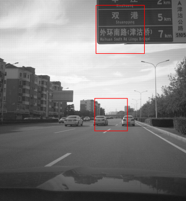
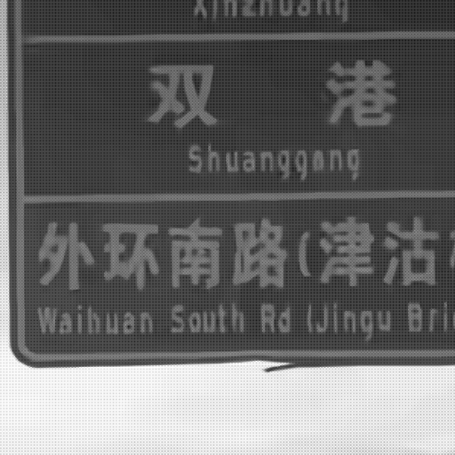
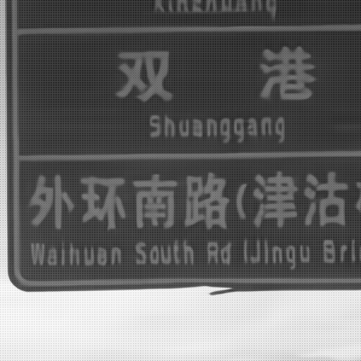
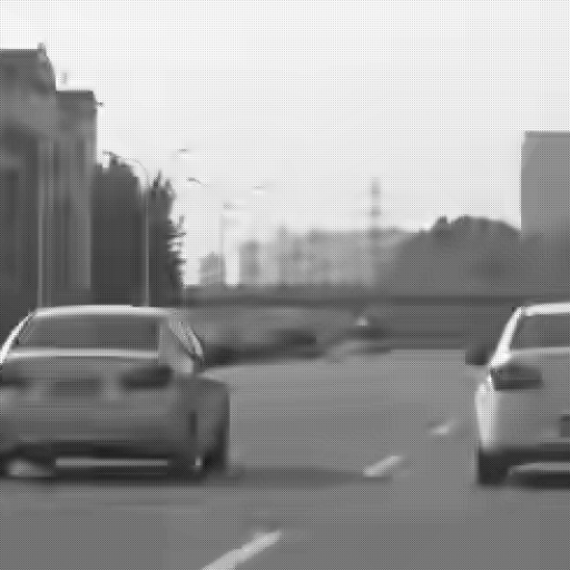
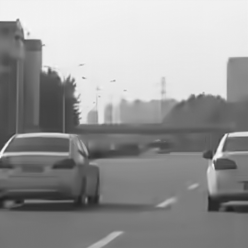
$12\text{\,}\mathrm{b}\mathrm{p}\mathrm{p}$	$0.015\text{\,}\mathrm{b}\mathrm{p}\mathrm{p}$	$0.015\text{\,}\mathrm{b}\mathrm{p}\mathrm{p}$	$0.016\text{\,}\mathrm{b}\mathrm{p}\mathrm{p}$	$0.017\text{\,}\mathrm{b}\mathrm{p}\mathrm{p}$	$0.015\text{\,}\mathrm{b}\mathrm{p}\mathrm{p}$
-	$44.15\text{\,}\mathrm{dB}$	$44.28\text{\,}\mathrm{dB}$	$44.79\text{\,}\mathrm{dB}$	$45.14\text{\,}\mathrm{dB}$	$46.35\text{\,}\mathrm{dB}$
Ground Truth	HEVC-8bits	HEVC-10bits	VVC-8bits	VVC-12bits	Ours

Figure 8: Qualitative Visualization. Reconstructions and close-ups of the HEVC, VVC, and our method. Corresponding bpp and PSNR are marked. Gamma correction and brightness adjustment have been applied for a better view. Zoom for better details.

Implementation convenience. Given that our method does not require paired RAW and RGB samples to train the invISP for the generation of simRAW images, it is much easier for practitioners to use our method to promote RAW-domain tasks. Furthermore, generated simRAW images can also be used to train/finetune models for other tasks, such as the segmentation method discussed in the supplementary material.

Note that most of the domain adaptation approaches [62, 18] need to modify the underlying model for each individual task manually. For example, Chen et al. [62] changed the predictor head of bounding box (bbox) and Li et al. [19] added bbox relevant loss functions which makes the migration to other tasks without bbox prediction impractical. In contrast, our method just retrains existing RGB-domain models (deployed in practice) to process RAW inputs. This makes our method suitable for various tasks, including detection and segmentation. Please see the supplementary material for more details.

5.3 RAW Image Compression (RIC)

This section presents results for RAW Image Compression (RIC) as a typical low-level task. Similar to Sec. 5.2, we first demonstrate the feasibility and performance of simRAW-pretrained RIC, and then illustrate further improvement by few-shot finetuning using real RAW images.

Training RAW-domain RIC. We use unpaired RGB and RAW samples from Flicker2W and iPhone RAW datasets to train the Unpaired Cycle R2R and generate simRAW images. Given that we do not need to label the semantic cues for high-level tasks, we use less than $1\text{\,}\mathrm{\char 37\relax}$ (i.e., $10$) real and random RAW images to train our model. We present this challenging setting to demonstrate that our method can be fine-tuned using a small number of real images, which can be especially useful in real-world settings with limited training data.

Then we follow the same procedure in Sec. 5.1 to convert native RGB images in Flicker2W [63] to simRAW images (i.e. simRAW_f) for the training of lossy and lossless RIC models, marked as Lossy RIC-$1\text{\,}\mathrm{\char 37\relax}$ and Lossless RIC-$1\text{\,}\mathrm{\char 37\relax}$. We also fine-tune these simRAW-pretrained models with more real RAW data for further improvement (see Lossy and Lossless RIC-$100\text{\,}\mathrm{\char 37\relax}$).

All RIC training threads run on a single NVIDIA 3090Ti GPU for a total of $400$ epochs. Adam optimizer with the learning rate of $10^{-4}$ and batch size of 8 for each iteration. For lossy RIC, eight models are trained to provide $8$ different bit rates (or quality levels). A pre-trained high-rate model is used to initialize the weights and to train a model for the lossless mode.

Comparative studies of Lossy RIC. We compare our Lossy RIC with HEVC Intra and VVC Intra through the compression of MultiRAW test set. Because traditional video codecs cannot handle the RAW images directly, we decompose the spectral channels (RG_rG_bB) of a RAW image into an RGB image i.e., R$G_{r}$B and a residual image r_g = G_b - G_r following the Apple ProRes RAW setting, which then can be encoded by HEVC Intra, VVC Intra, respectively. Here, we apply the reference software models of HEVC and VVC for intra-compression (i.e., HEVC 16.22 and VTM 11.0). Note that we perform the linearization on the RAW image by scaling the pixels in [0, 1] range. We then scale them to different bit depths before feeding them into the HEVC or VVC Intra coder. Since both HEVC and VVC can support higher bit depth beyond 8-bit precision, we have also tried out the 10-bit and 12-bit precision. As such, we can alleviate the quantization loss as much as possible. All other parameters in HEVC and VVC intra-encoders are kept same as default.

Figure 7 shows the rate-distortion performance of RAW image compression. As seen, even simRAW-pretrained lossy RIC (i.e., Lossy RIC-$1\text{\,}\mathrm{\char 37\relax}$) largely outperforms state-of-the-art 12-bit VVC. When we use more real RAW images to finetune the pretrained lossy RIC, the compression efficiency is further improved as reported for Lossy RIC-$50\text{\,}\mathrm{\char 37\relax}$ and Lossy RIC-$100\text{\,}\mathrm{\char 37\relax}$ that provide 2–3 dB PSNR gains over $8\text{\,}\mathrm{b}\mathrm{i}\mathrm{t}\mathrm{s}$ HEVC Intra, 1–2 dB gains over $12\text{\,}\mathrm{b}\mathrm{i}\mathrm{t}\mathrm{s}$ VVC Intra across a wide bit rate range.

Figure 8 presents the reconstructions and closeups generated by the HEVC Intra, VVC Intra, and our Lossy RIC-$100\text{\,}\mathrm{\char 37\relax}$. As seen, our method noticeably improves the subjective quality with sharper textures and lesser noise.

TABLE IV: Ablation of modular components of Unpaired CycleR2R. KL divergence was assessed between real and simulated RAW images. Additionally, Recall and Average Precision (AP) metrics were evaluated using various RAW-domain detectors. These detectors were trained on simRAW images, generated by adapting modular settings in Unpaired CycleR2R, including Auto White Balance (AWB), Brightness Adjustment (BA) and Color Correction (CC), Illumination Estimation Module (IEM) and variance loss $\mathcal{L}_{var}$.

Method	AWB	BA	CC	IEM+$\mathcal{L}_{var}$	KL	Recall	AP
InvGamma [25]	-	-	-	-	0.25	68.6	47.7
CycleISP [14]	-	-	-	-	0.08	71.6	52.7
CIE-XYZ Net [15]	-	-	-	-	0.13	72.2	53.0
MBISPLD [16]	-	-	-	-	0.11	73.0	53.7
Unpaired CycleR2R	✓				0.12	71.9	53.6
	✓	✓			0.10	72.5	54.9
	✓	✓	✓		0.09	74.9	56.1
	✓	✓	✓	✓	0.06	76.1	59.1

Comparative studies of Lossless RIC. Table III shows a comparison of our approach and other lossless codecs for the test samples in MultiRAW set, in terms of the bits per pixel (BPP). For PNG, JPEG XL, and FLIF designed for RGB images, we use the same evaluation strategy by splitting it into two images for compression. First, our Lossless RIC-$1\text{\,}\mathrm{\char 37\relax}$ trained on simRAW${}_{\textrm{f}}$ only already outperforms PNG (a widely-used RGB compressor) with 35–$74\text{\,}\mathrm{\char 37\relax}$ reduction in BPP and CinemaDNG (a professional RAW compressor) with 45–$96\text{\,}\mathrm{\char 37\relax}$ reduction in BPP, for three different cameras. Compared with JPEG XL and FLIF, our method offers up to $48\text{\,}\mathrm{\char 37\relax}$ reduction in BPP, but our method runs much faster for both encoding and decoding. Furthermore, the small gap of ($<$2\text{\,}\mathrm{\char 37\relax}$$) between Lossless RIC-$100\text{\,}\mathrm{\char 37\relax}$ and Lossless RIC-$1\text{\,}\mathrm{\char 37\relax}$ reveals that our Unpaired CycleR2R is capable of characterizing and embedding sufficient RAW-domain knowledge using a very small amount of real RAW images. Furthermore, the simRAW images produced by our invISP are able to train a generic lossless RAW image compressor. This makes our solution very attractive for practical situations with limited real training data.

6 Ablation Studies

In this section, we first provide additional discussion on the modular components of invISP. Then we study the impact of gamma correction and illumination on RAW-domain detection. Finally, we presents the progressive decoding ability of our lossless RIC and $\rho$-Vision’s hardware implementation.

6.1 Modular Components of Unpaired CycleR2R

Table IV employs the Kullback-Leibler (KL) divergence alongside Recall and Average Precision (AP) to evaluate the impact of modular components within the Unpaired CycleR2R framework. The KL divergence assesses the distribution similarity between the color channels of simulated (simRAW) and real captured RAW images, with lower values indicating higher resemblance. This statistical measure is crucial for determining the realism of simRAW images utilized for training vision models. In addition to the KL divergence, Recall, and AP metrics are calculated by executing the task upon the same real RAW dataset. Here, various detectors are trained on simRAW images by activating or deactivating certain modules of our model. These metrics demonstrate that each module significantly influences task accuracy. The Illumination Estimation Module (IEM), in particular, markedly increases the AP from $56.1\text{\,}\mathrm{\char 37\relax}$ to $59.1\text{\,}\mathrm{\char 37\relax}$. This improvement is credited to IEM’s advanced simulation of diverse lighting conditions, which is more representative of real-world scenarios than traditional methods that often rely on fixed illumination settings for ISP/invISP modeling. We give some visualization samples in the Supplementary, showcasing the module’s contribution to producing training data that closely mirrors genuine imaging conditions.

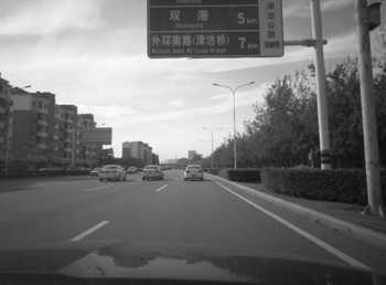
$0.08\text{\,}\mathrm{b}\mathrm{p}\mathrm{p}$ / $36.77\text{\,}\mathrm{dB}$	$0.14\text{\,}\mathrm{b}\mathrm{p}\mathrm{p}$ / $40.07\text{\,}\mathrm{dB}$	$0.38\text{\,}\mathrm{b}\mathrm{p}\mathrm{p}$ / $44.13\text{\,}\mathrm{dB}$	$1.34\text{\,}\mathrm{b}\mathrm{p}\mathrm{p}$ / $49.96\text{\,}\mathrm{dB}$	$5.13\text{\,}\mathrm{b}\mathrm{p}\mathrm{p}$ / GT
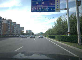
$0.15\text{\,}\mathrm{s}$ / $28.67\text{\,}\mathrm{dB}$	$0.26\text{\,}\mathrm{s}$ / $31.43\text{\,}\mathrm{dB}$	$0.37\text{\,}\mathrm{s}$ / $34.60\text{\,}\mathrm{dB}$	$0.52\text{\,}\mathrm{s}$ / $38.24\text{\,}\mathrm{dB}$	$0.68\text{\,}\mathrm{s}$ / GT

Figure 9: Progressive Decoding. The gradual reconstruction of RAW images and their corresponding RGB images converted by an in-camera ISP. Bits per pixel (bpp) / PSNR (dB) is shown under RAW images. Decoding latency (s) / PSNR (dB) is also listed below RGB images. PSNR is derived against the GT (ground truth). Gamma correction and brightness adjustment have been applied for a better view. Zoom for more details.

6.2 Gamma Correction

TABLE V: Impact of Gamma Correction (GC) on object detection for different cameras and different object classes.

Domain	Camera	Vehicle	Person	Tr. Sign	Tr. Light	mAP
RGB	i-12	82.6	34.9	72.7	54.0	61.1
RAW w/o GC		79.2	25.3	70.2	48.6	55.8
RAW w/ GC		81.1	33.5	73.8	55.0	60.8
RGB	HW-12	75.3	38.4	62.2	49.5	56.4
RAW w/o GC		74.3	33.7	61.4	49.4	54.7
RAW w/ GC		75.5	39.4	62.0	50.9	57.0
RGB	asi-14	76.2	34.0	66.4	60.7	58.3
RAW w/o GC		60.2	18.5	49.7	46.8	43.8
RAW w/ GC		79.0	42.2	71.8	63.8	64.2

• i-12 $\leftarrow$ iPhone XSmax ($12\text{\,}\mathrm{b}\mathrm{i}\mathrm{t}\mathrm{s}$); HW-12 $\leftarrow$ Huawei P30pro ($12\text{\,}\mathrm{b}\mathrm{i}\mathrm{t}\mathrm{s}$); asi-14 $\leftarrow$ asi 294mcpro ($14\text{\,}\mathrm{b}\mathrm{i}\mathrm{t}\mathrm{s}$).

• Tr. Sign $\leftarrow$ Traffic Sign; Tr. Light $\leftarrow$ Traffic Light.

We prove analytically in Sec. 4.1.2 that directly feeding linear RAW images into the detector typically leads to inferior detection performance. We then suggest the gamma correction approach adjusts the input distribution and subsequently boosts the performance of RAW-domain detection. Here we offer a quantitative evaluation of the gamma correction.

For a fair comparison, we train three detectors sharing the same head (YOLOv3 [12]) and backbone (MobileNetV2 [61]) using the training samples in the proposed MultiRAW dataset. Specifically, we train an RGB-domain detector (i.e., RGB in Table V) using the RGB images that are converted from the RAW samples with in-camera ISP, and use it to test RGB images as well. We also train two RAW-domain detectors where one option, RAW w/ GC in Table V, applies the gamma correction to adjust training RAW samples prior to the training, and the other one, RAW w/o GC in Table V, keeps using the same RAW samples without change.

As seen, without gamma correction, the performance of the RAW-domain detector is inferior to that of the RGB-domain detector with a noticeable gap. The gamma correction significantly improves the detection results even exceeding the RGB-domain model, further confirming the analytical proof in Sec. 4.1.2. The performance improvement is larger for asi 294mcpro camera sensor that has a 14-bit dynamic range, suggesting that fine-grained spatial details in shadow and highlight parts can be well retained in high-bit-precision RAW samples for better object detection.

6.3 Illumination Influence on Detection Accuracy

TABLE VI: Comparative analysis of object detection performance under different illumination conditions across various object sizes.

Scenarios	Domain	$\textbf{mAP}_{\text{small}}$	$\textbf{mAP}_{\text{medium}}$	$\textbf{mAP}_{\text{large}}$	mAP
Day	RGB	19.1	54.9	73.6	58.5
	RAW	21.2	57.8	74.7	60.5
Night	RGB	17.0	49.1	63.1	56.1
	RAW	28.2	54.5	67.7	59.8

Facing the Sun
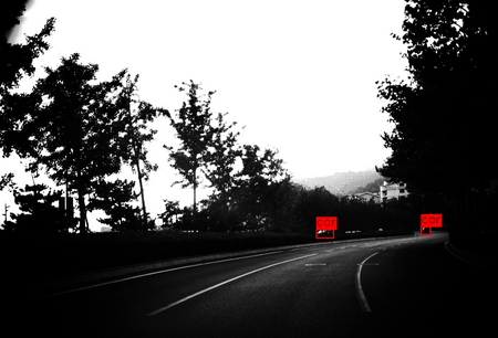
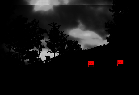
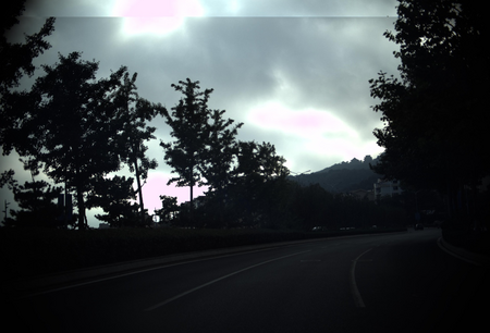
Night Lens Flare
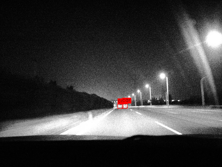
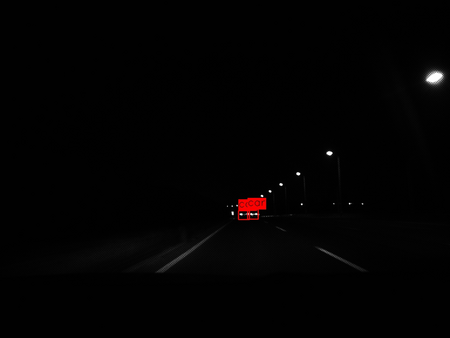
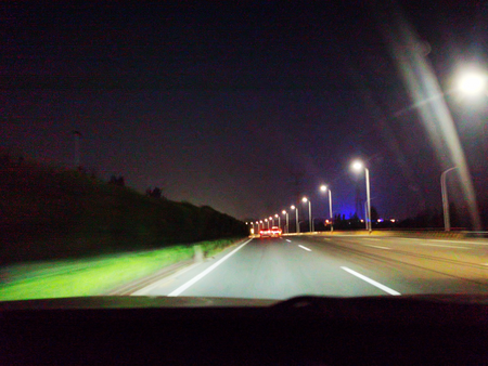
Complex Lighting
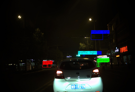
Lower 8 Bits of RAW Image	Higher 8 Bits of RAW Image	8-bit RGB

Figure 10: Visualizing the detection results under challenging illumination conditions for the RAW domain and RGB domain methods. The first column displays the lower 8 bits of the RAW data, which retains the shadow details often lost in standard 8-bit RGB images due to brightness clipping. The second (middle) column presents the higher 8 bits of the RAW data, which contains the details in the bright areas. The third column uses the 8-bit RGB for detection. Detection results are overlaid for comparative study.

The influence of illumination conditions on object detection accuracy was systematically evaluated across various object scales. The performance metrics, detailed in Table VI, reveal notable improvements when using RAW data for detection, especially under complex nighttime conditions (+3.7). This improvement is particularly pronounced for small objects (+11.2), where the RAW format’s extended dynamic range facilitates the discernment of details often lost in standard 8-bit RGB images due to brightness clipping or overexposure.

Figure 10 further visualizes the detection results under various challenging illumination scenarios, such as direct sunlight, night lens flare, and complex lighting with multiple sources. As seen, RAW-domain processing can better preserve details in both bright and shadow areas which are typically overlooked in standard 8-bit RGB images due to brightness clipping or overexposure.

6.4 Progressive Decoding

Our lossless RIC model supports progressive decoding to refine the image resolution gradually, which enables the low-resolution preview of high-resolution RAW and RGB images (converted by the in-camera ISP). Such a prompt low-resolution preview (see the visualization in Fig. 9) is a useful add-on function for applications like professional photography. As also shown in Fig. 9, we can observe the restoration of high-frequency details gradually. Another useful takeaway of such progressive decoding is its inherent network transmission friendliness, with which we can still decode partial bitstream received at the client for display or consumption [64].

6.5 Hardware Implementation

We deployed our $\rho$-Vision framework on the Axera-Tech AX620A SoC, which facilitated a direct comparison between RAW-domain visual computing and conventional ISP processing methods. Utilizing YOLOv8-S and the MultiRAW dataset as our benchmark, the experimental outcomes underscore the superiority of $\rho$-Vision. Specifically, we observed a 3% increase in detection accuracy, coupled with substantial reductions in latency (72%), power consumption (62%), and memory usage (36%). Notably, these enhancements were achieved without necessitating complex modifications to the network model architecture. The benefits of our approach become even more evident under challenging conditions, such as in low-light and high dynamic range scenarios. Detailed results and further analyses can be found in our supplementary materials.

7 Conclusion

In this paper, we demonstrate that performing high-level vision tasks and low-level image compression on the camera RAW images is practically feasible and efficient. In this way, the ISP modules, which are incorporated into cameras for decades, can be completely bypassed, thus promising an alternative and encouraging paradigm for image/video acquisition, processing, and display. Our Unpaired CycleR2R is able to effectively characterize, embed, and transfer necessary knowledge between unpaired RGB and camera RAW samples to build the mapping between RGB and RAW spaces in an unsupervised manner. This enables us to conveniently generate sufficient simRAW images to retain/finetune popular RGB-domain neural models deployed in existing products for RAW-domain task executions. We present extensive experiments on high-level object detection and low-level image compression tasks in the RAW domain, which show better performance can be achieved in RAW domain compared to the RGB domain. One potential future direction is to develop similar models for processing RAW videos. We will make our MultiRAW dataset and Unpaired CycleR2R code publicly accessible for reproducible research at https://njuvision.github.io/rho-vision upon the acceptance of this work.

8 Acknowledgement

We are very grateful for those pioneering explorations in [15, 16, 14] which inspire this work.

Zhihao Li (Member, IEEE) received his B.S. and Master degrees in the School of Electronic Science and Engineering from Nanjing University, Jiangsu, China, in 2020 and 2023 respectively. His current research focuses on raw image signal processing and event camera. He is a co-recipient of the 2nd International Illumination Estimation Challenge and the CVPRW 2022 Night Image Rendering Challenge Runner-up solution.

Ming Lu (Member, IEEE) is an Associate Researcher in the School of Electronic Science and Engineering, Nanjing University, Jiangsu, China. He received his B.S. and Ph.D. degrees in the School of Electronic Science and Engineering from Nanjing University, Jiangsu, China, in 2016 and 2023 respectively. His current research focuses on deep learning-based image/video coding. He is a co-recipient of the 2018 ACM SIGCOMM Student Research Competition Finalist, the 2020 IEEE MMSP Image Compression Grand Challenge Best Performing Solution, and the 2023 IEEE WACV Best Algorithms Paper Award.

Xu Zhang (Member, IEEE) is a Lecturer with the School of Computing, Faculty of Engineering and Physical Sciences, University of Leeds, LS2 9JT, United Kingdom. He received the BS degree in communication engineering from the Beijing University of Posts and Telecommunications, China, in 2012 and the Ph.D. degree in computer science from the Department of Computer Science and Technology, Tsinghua University, China, in 2017. He worked at Nanjing University and the University of Exeter before joining the University of Leeds. His research interests include AI for computing and networking, multimedia communication, and Internet of Things. He was a recipient of the EU Marie Skłodowska-Curie Individual Fellowships and a co-recipient of the 2019 IEEE Broadcast Technology Society Best Paper Award.

Xin Feng (Senior Member, IEEE) received her B.S. degree in computer science and technology from Chongqing University in 2004. She conducted her postgraduate study from 2004 to 2006 and got the Ph.D. degree in computer applications from Chongqing University in 2011. She is currently an associate professor at Chongqing University of Technology. She studied at New York University as a postdoctoral from 2014 to 2016. Her research falls in the area of computer vision, image, and video processing. Her current research interests cover object detection, and multi-object tracking for visual perception in auto-driving.

M. Salman Asif (Senior Member, IEEE) received the B.Sc. degree from the University of Engineering and Technology, Lahore, Pakistan, and the M.S and Ph.D. degrees from the Georgia Institute of Technology, Atlanta, GA, USA. He is currently an associate professor with the University of California Riverside, Riverside, CA, USA. Prior to that, he was a Postdoctoral Researcher with Rice University, Houston, TX, USA, and a Senior Research Engineer with Samsung Research America, Dallas. His research interests include computational imaging, signal/image processing, computer vision, and machine learning. He was the recipient of the NSF CAREER Award, Google Faculty Award, Hershel M. Rich Outstanding Invention Award, and UC Regents Faculty Fellowship and Development Awards.

Zhan Ma (Senior Member, IEEE) is a Professor in the School of Electronic Science and Engineering, Nanjing University, Jiangsu, 210093, China. He received his Ph.D. from New York University, New York, in 2011 and his B.S. and M.S. from the Huazhong University of Science and Technology, Wuhan, China, in 2004 and 2006 respectively. From 2011 to 2014, he has been with Samsung Research America, Dallas, TX, and Futurewei Technologies, Inc., Santa Clara, CA, respectively. His research focuses include learned image/video coding and computational imaging. He was awarded the 2018 PCM Best Paper Finalist, the 2019 IEEE Broadcast Technology Society Best Paper Award, the 2020 IEEE MMSP Grand Challenge Best Image Coding Solution, the 2023 IEEE WACV Best Algorithms Paper Award, and the 2023 IEEE Circuits and Systems Society Outstanding Young Author Award.

References

- [1] X. Lin, X. Wang, and W. Yang, “From motion to magic: Real-time virtual-real stage effects via 3d motion capture,” Metaverse, vol. 4, no. 2, 2023.
- [2] R. Wang and N. Hua, “The image artistry of vr film “killing a superstar”,” Metaverse, vol. 4, no. 2, 2023.
- [3] Y. Yang, Z. Hao, W. Peng, K. Tang, and M. Fang, “Multi-task super resolution method for vector field critical points enhancement,” Metaverse, vol. 3, no. 1, p. 8, 2022.
- [4] X. Zhang, Y. Zhao, G. Min, W. Miao, H. Huang, and Z. Ma, “Intelligent video ingestion for real-time traffic monitoring,” ACM Trans. Sen. Netw., vol. 18, no. 3, sep 2022.
- [5] T. D. Räty, “Survey on contemporary remote surveillance systems for public safety,” IEEE Transactions on Systems, Man, and Cybernetics, Part C (Applications and Reviews), vol. 40, no. 5, pp. 493–515, 2010.
- [6] R. Okuda, Y. Kajiwara, and K. Terashima, “A survey of technical trend of adas and autonomous driving,” in Technical Papers of 2014 International Symposium on VLSI Design, Automation and Test. IEEE, 2014, pp. 1–4.
- [7] D. J. Brady, L. Fang, and Z. Ma, “Deep learning for camera data aquisition, control and image estimation,” Advances in Optics and Photonics, Sept. 2020.
- [8] J. Honovich, “Live video monitoring usage statistics,” 2015. [Online]. Available: {https://ipvm.com/reports/live-video-monitoring-usage-statistics}
- [9] M. Buckler, S. Jayasuriya, and A. Sampson, “Reconfiguring the imaging pipeline for computer vision,” in Proceedings of the IEEE International Conference on Computer Vision, 2017, pp. 975–984.
- [10] AI Camera, “Ambarella unveils two new ai chip families for 4k security cameras,” 2021. [Online]. Available: {https://venturebeat.com/ai/ambarella-unveils-two-new-ai-chip-families-for-4k-security-cameras/}
- [11] J. Deng, W. Dong, R. Socher, L.-J. Li, K. Li, and L. Fei-Fei, “ImageNet: A Large-Scale Hierarchical Image Database,” in CVPR09, 2009.
- [12] J. Redmon, S. Divvala, R. Girshick, and A. Farhadi, “You only look once: Unified, real-time object detection,” in 2016 IEEE Conference on Computer Vision and Pattern Recognition (CVPR), 2016, pp. 779–788.
- [13] M. Lu and Z. Ma, “High-efficiency lossy image coding through adaptive neighborhood information aggregation,” arXiv preprint arXiv:2204.11448, 2022.
- [14] S. W. Zamir, A. Arora, S. Khan, M. Hayat, F. S. Khan, M.-H. Yang, and L. Shao, “Cycleisp: Real image restoration via improved data synthesis,” in Proceedings of the IEEE/CVF Conference on Computer Vision and Pattern Recognition, 2020, pp. 2696–2705.
- [15] M. Afifi, A. Abdelhamed, A. Abuolaim, A. Punnappurath, and M. S. Brown, “CIE XYZ Net: Unprocessing images for low-level computer vision tasks,” IEEE Transactions on Pattern Analysis and Machine Intelligence, 2021.
- [16] M. V. Conde, S. McDonagh, M. Maggioni, A. Leonardis, and E. Pérez-Pellitero, “Model-based image signal processors via learnable dictionaries,” in AAAI, 2022.
- [17] J.-Y. Zhu, T. Park, P. Isola, and A. A. Efros, “Unpaired image-to-image translation using cycle-consistent adversarial networks,” in Proceedings of the IEEE international conference on computer vision, 2017, pp. 2223–2232.
- [18] M. Hnewa and H. Radha, “Multiscale domain adaptive yolo for cross-domain object detection,” in 2021 IEEE International Conference on Image Processing (ICIP). IEEE, 2021, pp. 3323–3327.
- [19] Y.-J. Li, X. Dai, C.-Y. Ma, Y.-C. Liu, K. Chen, B. Wu, Z. He, K. Kitani, and P. Vajda, “Cross-domain adaptive teacher for object detection,” in Proceedings of the IEEE/CVF Conference on Computer Vision and Pattern Recognition, 2022, pp. 7581–7590.
- [20] H. C. Karaimer and M. S. Brown, “A software platform for manipulating the camera imaging pipeline,” in European Conference on Computer Vision. Springer, 2016, pp. 429–444.
- [21] N. A, “Understanding the image signal processor and isp tuning - pathpartnertech.” [Online]. Available: https://www.pathpartnertech.com/camera-tuning-understanding-the-image-signal-processor-and-isp-tuning/
- [22] R. M. Nguyen and M. S. Brown, “Raw image reconstruction using a self-contained srgb-jpeg image with only 64 kb overhead,” in Proceedings of the IEEE Conference on Computer Vision and Pattern Recognition, 2016, pp. 1655–1663.
- [23] T. Brooks, B. Mildenhall, T. Xue, J. Chen, D. Sharlet, and J. T. Barron, “Unprocessing images for learned raw denoising,” in Proceedings of the IEEE Conference on Computer Vision and Pattern Recognition, 2019, pp. 11 036–11 045.
- [24] Z. Li, H. Liu, L. Yang, and Z. Ma, “In-camera raw compression: A new paradigm from image acquisition to display,” in 54th Asilomar Conference on Signals, Systems and Computers, 2020.
- [25] S. Koskinen, D. Yang, and J.-K. Kämäräinen, “Reverse imaging pipeline for raw rgb image augmentation,” in 2019 IEEE International Conference on Image Processing (ICIP). IEEE, 2019, pp. 2896–2900.
- [26] T. Plotz and S. Roth, “Benchmarking denoising algorithms with real photographs,” in 2017 IEEE Conference on Computer Vision and Pattern Recognition (CVPR). Los Alamitos, CA, USA: IEEE Computer Society, jul 2017, pp. 2750–2759. [Online]. Available: https://doi.ieeecomputersociety.org/10.1109/CVPR.2017.294
- [27] V. Bychkovsky, S. Paris, E. Chan, and F. Durand, “Learning photographic global tonal adjustment with a database of input / output image pairs,” in CVPR 2011, 2011, pp. 97–104.
- [28] V. Monga, Y. Li, and Y. C. Eldar, “Algorithm unrolling: Interpretable, efficient deep learning for signal and image processing,” IEEE Signal Processing Magazine, vol. 38, no. 2, pp. 18–44, 2021.
- [29] F. Yu, H. Chen, X. Wang, W. Xian, Y. Chen, F. Liu, V. Madhavan, and T. Darrell, “Bdd100k: A diverse driving dataset for heterogeneous multitask learning,” in Proceedings of the IEEE/CVF Conference on Computer Vision and Pattern Recognition, 2020, pp. 2636–2645.
- [30] A. Abdelhamed, M. A. Brubaker, and M. S. Brown, “Noise flow: Noise modeling with conditional normalizing flows,” in Proceedings of the IEEE/CVF International Conference on Computer Vision, 2019, pp. 3165–3173.
- [31] N. Ohta and A. Robertson, “Cie standard colorimetric system,” Colorimetry: Fundamentals and applications, pp. 63–114, 2006.
- [32] J. M. Hollas, Modern spectroscopy. John Wiley & Sons, 2004.
- [33] X. Li, B. Gunturk, and L. Zhang, “Image demosaicing: A systematic survey,” in Visual Communications and Image Processing 2008, vol. 6822. SPIE, 2008, pp. 489–503.
- [34] A. Gijsenij, T. Gevers, and J. van de Weijer, “Computational color constancy: Survey and experiments,” IEEE Transactions on Image Processing, vol. 20, no. 9, pp. 2475–2489, 2011.
- [35] M. Afifi and M. S. Brown, “What else can fool deep learning? addressing color constancy errors on deep neural network performance,” in 2019 IEEE/CVF International Conference on Computer Vision, ICCV 2019, Seoul, Korea (South), October 27 - November 2, 2019. IEEE, 2019, pp. 243–252. [Online]. Available: https://doi.org/10.1109/ICCV.2019.00033
- [36] G. D. Finlayson, M. Mackiewicz, and A. Hurlbert, “Color correction using root-polynomial regression,” IEEE Transactions on Image Processing, vol. 24, no. 5, pp. 1460–1470, 2015.
- [37] Z. Zhou, N. Sang, and X. Hu, “Global brightness and local contrast adaptive enhancement for low illumination color image,” Optik, vol. 125, no. 6, pp. 1795–1799, 2014.
- [38] S. Wolf, Color correction matrix for digital still and video imaging systems. National Telecommunications and Information Administration Washington, DC, 2003.
- [39] H. Farid, “Blind inverse gamma correction,” IEEE transactions on image processing, vol. 10, no. 10, pp. 1428–1433, 2001.
- [40] M. Stokes, “A standard default color space for the internet-srgb,” http://www. color. org/contrib/sRGB. html, 1996.
- [41] F. Drago, K. Myszkowski, T. Annen, and N. Chiba, “Adaptive logarithmic mapping for displaying high contrast scenes,” in Computer graphics forum, vol. 22, no. 3. Wiley Online Library, 2003, pp. 419–426.
- [42] J. T. Barron and Y.-T. Tsai, “Fast fourier color constancy,” in Proceedings of the IEEE conference on computer vision and pattern recognition, 2017, pp. 886–894.
- [43] B. Xu, N. Wang, T. Chen, and M. Li, “Empirical evaluation of rectified activations in convolutional network,” arXiv preprint arXiv:1505.00853, 2015.
- [44] T. Park, A. A. Efros, R. Zhang, and J.-Y. Zhu, “Contrastive learning for unpaired image-to-image translation,” in European conference on computer vision. Springer, 2020, pp. 319–345.
- [45] J. Liu, J. Tang, and G. Wu, “Adadm: Enabling normalization for image super-resolution,” arXiv preprint arXiv:2111.13905, 2021.
- [46] T.-Y. Lin, P. Dollár, R. Girshick, K. He, B. Hariharan, and S. Belongie, “Feature pyramid networks for object detection,” in Proceedings of the IEEE CVPR, 2017, pp. 2117–2125.
- [47] Q. Chen, Y. Wang, T. Yang, X. Zhang, J. Cheng, and J. Sun, “You only look one-level feature,” in Proceedings of the IEEE/CVF conference on computer vision and pattern recognition, 2021, pp. 13 039–13 048.
- [48] R. Girshick, “Fast r-cnn,” in Proceedings of the IEEE international conference on computer vision, 2015, pp. 1440–1448.
- [49] S. Ren, K. He, R. Girshick, and J. Sun, “Faster r-cnn: Towards real-time object detection with region proposal networks,” Advances in neural information processing systems, vol. 28, 2015.
- [50] Y. Wu and K. He, “Group normalization,” in Proceedings of the European conference on computer vision (ECCV), 2018, pp. 3–19.
- [51] J. Wang, K. Sun, T. Cheng, B. Jiang, C. Deng, Y. Zhao, D. Liu, Y. Mu, M. Tan, X. Wang et al., “Deep high-resolution representation learning for visual recognition,” IEEE transactions on pattern analysis and machine intelligence, vol. 43, no. 10, pp. 3349–3364, 2020.
- [52] S. Ioffe and C. Szegedy, “Batch normalization: Accelerating deep network training by reducing internal covariate shift,” in International conference on machine learning. PMLR, 2015, pp. 448–456.
- [53] Y. Liu, J. Ge, C. Li, and J. Gui, “Delving into variance transmission and normalization: Shift of average gradient makes the network collapse,” arXiv preprint arXiv:2103.11590, 2021.
- [54] T. Chen, H. Liu, Z. Ma, Q. Shen, X. Cao, and Y. Wang, “End-to-end learnt image compression via non-local attention optimization and improved context modeling,” IEEE Trans. Image Processing, vol. 30, pp. 3179–3191, 2021.
- [55] M. Lu, P. Guo, H. Shi, C. Cao, and Z. Ma, “Transformer-based image compression,” IEEE Data Compression Conf., Jan. 2022.
- [56] J. Liu, C.-H. Wu, Y. Wang, Q. Xu, Y. Zhou, H. Huang, C. Wang, S. Cai, Y. Ding, H. Fan et al., “Learning raw image denoising with bayer pattern unification and bayer preserving augmentation,” in Proceedings of the IEEE Conference on Computer Vision and Pattern Recognition Workshops, 2019, pp. 0–0.
- [57] F. Mentzer, E. Agustsson, M. Tschannen, R. Timofte, and L. V. Gool, “Practical full resolution learned lossless image compression,” in Proceedings of the IEEE/CVF conference on computer vision and pattern recognition, 2019, pp. 10 629–10 638.
- [58] S. Cao, C.-Y. Wu, and P. Krähenbühl, “Lossless image compression through super-resolution,” arXiv preprint arXiv:2004.02872, 2020.
- [59] F. Mentzer, E. Agustsson, M. Tschannen, R. Timofte, and L. V. Gool, “Practical full resolution learned lossless image compression,” in Proceedings of the IEEE/CVF conference on computer vision and pattern recognition, 2019, pp. 10 629–10 638.
- [60] S. Cao, C.-Y. Wu, and P. Krähenbühl, “Lossless image compression through super-resolution,” arXiv preprint arXiv:2004.02872, 2020.
- [61] M. Sandler, A. Howard, M. Zhu, A. Zhmoginov, and L.-C. Chen, “Mobilenetv2: Inverted residuals and linear bottlenecks,” in Proceedings of the IEEE conference on computer vision and pattern recognition, 2018, pp. 4510–4520.
- [62] Y. Chen, W. Li, C. Sakaridis, D. Dai, and L. Van Gool, “Domain adaptive faster r-cnn for object detection in the wild,” in Proceedings of the IEEE conference on computer vision and pattern recognition, 2018, pp. 3339–3348.
- [63] J. Liu, G. Lu, Z. Hu, and D. Xu, “A unified end-to-end framework for efficient deep image compression,” arXiv preprint arXiv:2002.03370, 2020.
- [64] H. Danyali and A. Mertins, “Highly scalable image compression based on spiht for network applications,” in Proceedings. International Conference on Image Processing, vol. 1, 2002, pp. I–I.