Temporal Saliency Detection Towards Explainable Transformer-based Timeseries Forecasting

Abstract

Despite the notable advancements in numerous Transformer-based models, the task of long multi-horizon time series forecasting remains a persistent challenge, especially towards explainability. Focusing on commonly used saliency maps in explaining DNN in general, our quest is to build attention-based architecture that can automatically encode saliency-related temporal patterns by establishing connections with appropriate attention heads. Hence, this paper introduces Temporal Saliency Detection (TSD), an effective approach that builds upon the attention mechanism and applies it to multi-horizon time series prediction. While our proposed architecture adheres to the general encoder-decoder structure, it undergoes a significant renovation in the encoder component, wherein we incorporate a series of information contracting and expanding blocks inspired by the U-Net style architecture. The TSD approach facilitates the multiresolution analysis of saliency patterns by condensing multi-heads, thereby progressively enhancing the forecasting of complex time series data. Empirical evaluations illustrate the superiority of our proposed approach compared to other models across multiple standard benchmark datasets in diverse far-horizon forecasting settings. The initial TSD achieves substantial relative improvements of 31% and 46% over several models in the context of multivariate and univariate prediction. We believe the comprehensive investigations presented in this study will offer valuable insights and benefits to future research endeavors.

1 Introduction

Time series forecasting empowers decision-making on chronological data, and performs an essential role in various research and industry fields such as healthcare [34], energy management [48], industrial automation [60], planning for infrastructure construction [43], economics and finance [44]. Time series observations can be a single sequence addressed by traditional time series forecasting approaches such as autoregressive integrated or exponentially weighted moving averages. However, actual time series data may consist of several channels as predictors for future forecasting and thus require more effective approaches. Multi-horizon prediction allows us to estimate a long sequence, optimizing intervened actions at multiple time steps in the future where performance improvements are precious. Hence, a significant challenge for time series forecasting is to develop practical models dealing with the heterogeneity of multi-channel time series data and produce accurate predictions in multi-horizon.

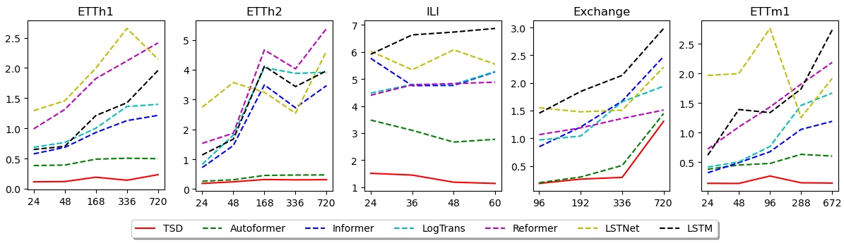
Figure 1: Multivariate time series forecasting comparison. The lower lines indicate better forecasting capacity. y-axis indicates the MSE loss while x-axis presents the prediction horizon.

Following the great success of attention mechanisms in machine translation, recent research has adapted it for time series forecasting [21, 66, 64, 6, 13, 63]. Self-attentions consider the local information that the models only utilize point-wise dependencies. Benefiting from the self-attention mechanism, Transformers achieve significant efficiencies in dependency modeling for sequential data, allowing for constructing more powerful large models. However, the forecasting problem is highly challenging in the long term and when many variables affect the target. First, detecting temporal dependencies directly from long-horizon time series is unreliable because the dependencies can be spread across many variables, and each variable tends to be different. Second, the canonical Transformer with self-attention requires high-power computing for long-term forecasting because of the quadratic complexity of the sequence length. Thus, to solve the computational hardware bottleneck, the previous Transformer-based predictive models mainly focused on improving the full self-attention to a sparse version. For the information aggregation, Autoformer adopts the time delay block to aggregate the similar sub-series from underlying periods rather than selecting scattered points by dot-product. The Auto-Correlation mechanism can simultaneously benefit the computation efficiency and information utilization from the inherent sparsity and sub-series-level representation aggregation. Despite the significantly improved performance, this approach has to sacrifice information usage because point connections lead to long-term time series forecasting bottlenecks that make it difficult to explain the trained models.

Towards explainability, saliency maps have been widely used to highlight important input features in model predictions to explain model behaviors in computer vision [62, 27, 9] and recently also apply for time series. In fact, [11] introduces the saliency-guided architecture that shows it works CNN and LSTM. However, it is still being determined whether such an approach will work with the recent transformer-based approach above, especially with the ones using sparsifying techniques. For example, [12] pointed out that attention-based methods can be insufficient for interpreting multivariate time-series data, e.g., saliency maps fail to reliably and accurately identify feature importance over time in time series data. We hypothesize that we need a technique to automatically encode the saliency-related temporal patterns via connecting to the suitable attention heads. Thus, we attempt to go beyond heuristic approaches such as Informer, e.g., sparse point-wise connection, Autoformer, e.g., sub-level-wise connection, and propose a generic architecture to empower forecasting models with automatic segment-wise interpolation. Inspired by saliency detection theory [65] in images and video recognition [53, 19], we propose a method to weigh the proper attention to possible emerging temporal patterns.

This method is realized as a learning architecture called Temporal Saliency Detection, which can be categorized into Transformer-family for far-horizon time series forecasting. Our proposed architecture still follows a general encoder-decoder structure but renovates the encoder component with a series of information contracting and expanding blocks inspired by U-Net style architecture [39]. The fundamental architecture of a U-net model comprises two distinct paths. The first path, referred to as the contracting path, encoder, or analysis path, closely resembles a conventional convolutional network and is responsible for extracting pertinent information from the input data. On the other hand, the second path, known as the expansion path, decoder, or synthesis path, encompasses up-convolutions and feature concatenations derived from the contracting path. This expansion process facilitates learning localized extracted information and concurrently enhances the output resolution. Subsequently, the augmented output passes through a final convolutional layer to generate the fully synthesized data. The resultant network exhibits an almost symmetrical configuration, endowing it with a U-like shape. To this end, similar to the latent diffusion models for high-resolution image synthesis [38], by allowing the attention mechanism and the information contraction to work in concert, our architecture can construct temporal saliency patterns through segment-wise aggregation. While U-Net style architecture [46] can pay the way for temporal saliency patterns to emerge like in [30], the challenge is how to match the performance of heuristics point-wise or sub-series-wise methods ( e.g., Informer, LogTrans, and Autorformer). The experiments in Section4 show that our approach can be competitive with several state-of-the-art methods as visually summarized in Figure 1. The contributions of the paper are summarized as follows:

• We introduce the Temporal Saliency Detection model as a harmonic combination between encoder-decoder structure and U-Net architecture to empower the far-horizon time series forecasting towards explainability.

• Our proposed approach discovers and aggregates temporal information at the segment-wise level. TSD consistently performs the prediction capacity in ten different multivariate-forecasting horizons.

• At the current initial investigation, TSD achieves a 31% and 46% relative improvement over compared models under multivariate and univariate time series forecasting on standard benchmarks.

2 Related Work

Long and Multi Horizon Time Series Forecasting has been a well-established research topic with a steadily growing number of publications due to its immense importance for real applications [25, 26]. Classical methods such as ARIMA [1], RNN [58, 61, 37], LSTM [2] and Prophet [50] serve as a standard baselines for forecasting. One of the most ubiquitous approaches in a wide variety of forecasting systems is deep time series which have been proven effective in both industries [28, 24] and academic [7, 51]. Amazon time series forecasting services build around DeepAR [42], which combines RNNs and autoregressive sliding methods to model the probabilistic future time points. Attention-based RNNs approaches capture temporal dependency for short and long term predictions [36, 45, 47]. CNN’s models for time series forecasting also provide a noticeable solution for periodically high-dimensional time series [56, 18, 17]. Another deep stack of fully-connected layers based on backward and forward residual links, named N-BEATS, was proposed by [29] and later improved by [3], called N-HITS, have empowered this research direction. Those forecasting approaches focus on temporal dependency modeling by current knowledge, recurrent connections, or temporal convolution.

Transformers Based on the Self-attention Mechanism, originating from the machine translation domain, have been successfully adapted to address different time series problems [17, 5, 45, 47, 22, 20]. Attention computation allows direct pair-wise comparison to any uncommon occurrence, e.g., sale seasons, and can model temporal dynamics inherently. However, pair-wise interactions make attention-based models suffer from the quadratic complexity of sequence length. Recent research, Reformer [14], Linformer [57], and Informer [66], proposes multiple variations of the canonical attention mechanisms have achieved superior forecasting while in parallel reducing the complexity of pair-wise interactions. Another exciting paper that belongs to the attention-based family of models is the Query Selector [15], where the idea of computing a sparse approximation of an attention matrix is exploited. Note that these forecasting models still rely on point-wise computation and aggregation. Nevertheless, those models have improved the self-attention mechanism from a full to a sparse version by sacrificing information utilization. In this context, we call them as sparsification architectures. Along the same line, YFormer [23] adjusted the Informer model by integrating a U-Net architecture into Informer’s ProbSparse Self-attention module. While it is also inspired by U-Net like us, YFormer inherits the problem of sacrificing the information utilization of Informer. Originated from the medical image segmentation problem, U-Net is capable of condensing input information to several intermediate embeddings and up-sampling them to the same resolutions as the input [39, 16, 10]. Apart from the image domain, the U-Net approach has proven noticeable results for sequence modeling [49] and time series segmentation [33].

Auto-correlation Mechanism A noticeable encoder-decoder architecture that utilizes Fourier transform is Autoformer [59] with decomposition capacities and an attention approximation. Autoformer is based on the series periodicity addressed in the stochastic process theory, where trend, seasonal, and other components are blended [4]. Hence, the model does not depend on temporal dependency as with the transformer-based solutions, but the auto-correlation emerging from data. The series-wise connections replace the point-wise representation.

Saliency has emerged as a prominent and effective method for enhancing interpretability, providing insights into why a trained model produces specific predictions for a given input. One approach to leveraging saliency is through saliency-guided training, which aims to diminish irrelevant features’ influence by reducing the associated gradient values. This is achieved by masking input features with low gradients and then minimizing the KL divergence between the outputs generated from the original input and the masked input, in addition to the main loss function. The effectiveness of the saliency approach has been demonstrated across various domains, including image analysis, language processing, and time series data [52, 41]. Another saliency technique involves extracting a series of images from sliding windows within time series data and defining a learnable mask based on these series images and their perturbed counterparts. This approach, series saliency, acts as an adaptive data augmentation method for training deep models [31]. In exploring perturbed versions of data, Parvatharaju et al. introduced a method called perturbation by prioritized replacement. This technique learns to emphasize the timesteps that contribute the most to the classifier’s prediction, indicating their importance [32]. Saadallah et al. tackled the challenge of searching for an optimal network architecture by considering candidate models from various deep neural network architectures. They dynamically selected the most suitable architecture in real-time using concept drift detection in time series data. Saliency maps were utilized to compute the region of competence for each candidate network [40].

3 Attention with Temporal Saliency

3.1 Problem Definition and Notation

A time series is composed of N univariate time series where each $i=1\dots N$, we have $y^{i}_{t}$ as a value of the univariate time series $i$ at time $t$. Given the look-back window $\tau$ , $x^{i}_{t}$ are exogenous inputs as associated co-variate values, e.g., day-of-the-week and hour-of-the-day. We can formulate the one-step-ahead prediction model as follows:

$$\hat{y}_{i,t+1}=f(y^{i}_{t-\tau\smalltriangleright t},x^{i}_{t-\tau\smalltriangleright t})$$ (1)

where $y^{i}_{t-\tau\smalltriangleright t}=\{y^{i}_{t-\tau},...,y^{i}_{t}\}$ and $x^{i}_{t-\tau\smalltriangleright t}=\{x^{i}_{t-\tau},...,x^{i}_{t}\}$.

As a common practice in transformer-based model, e.g., [57] and [59], the inputs $y^{i}_{t-\tau\smalltriangleright t},x^{i}_{t-\tau\smalltriangleright t}$ are encoded under a vector of hidden states $z$ to serve as the inputs for an attention block as the below step. The size $|z|$ is aligned with the number of input tokens for the transformer-based encoding block.

To prepare for the description of our architecture in the next section, we introduce two fundamental building blocks $\textrm{Conv}^{\downarrow}$ and $\textrm{Conv}^{\uparrow}$, with two following equations, e.g., downsampling and upsampling blocks, respectively. They are two parameterized sub-modules used in U-Net [39] style architecture. They both have two parameters, namely, $\mathcal{H}$ and $d$, which are the hidden input states and the drop-out parameter.

$$\textrm{Conv}^{\downarrow}(\mathcal{H},d)=\textrm{DropOut(MaxPool(ReLU(Conv1d}(\mathcal{H}))),d)$$ (2)

$$\textrm{Conv}^{\uparrow}(\mathcal{H},d)=\\ \textrm{DropOut(ConvT1d(ReLU(Conv1d}(\mathcal{H}))),d)$$ (3)

where ConvT1d is shorted for ConvTranspose1d.

3.2 Architecture for Temporal Saliency Detection

This section will introduce our proposed learning architecture illustrated in Figure 2.

The description will be followed from left to right according to the input flow. The critical novel aspect of this architecture is that the Temporal Saliency Detection ($\mathcal{TSD}$) block can work in tandem with the Temporal Self-Attention ($\mathcal{TSA}$) block. During the training process, the weights in both these blocks can be automatically adjusted to reveal temporal saliency maps in a similar fashion to semantic segmentation in computer vision. While our implementation is proven to outperform its competitors by a large margin, the saliency aspect will open the door for supporting the interpretability of our models as a natural next step for this work.

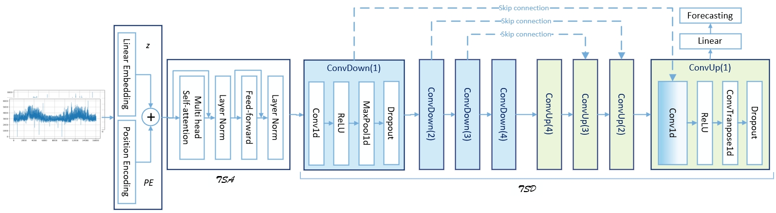
Figure 2: The high-level design of the Temporal Saliency Detection (TSD) model.

Time Series Tokenization

To prepare the input for the below $\mathcal{TSA}$ block, our architecture will encode time series into a Linear Embedding $z$ to make it compatible with token inputs of the attention module $\mathcal{TSA}$. Next, we use convolution block Conv1d to encode $z$ from input time series $(y^{i}_{t-\tau\smalltriangleright t},x^{i}_{t-\tau\smalltriangleright t})$. Note the number of the tokens $|z|$ is a hyper-parameter for our architecture (see Ablation study in Section 5).

$$z=\textrm{Conv1d}(y^{i}_{t-\tau\smalltriangleright t},x^{i}_{t-\tau\smalltriangleright t})$$ (4)

Temporal Self-Attention ($\mathcal{TSA}$)

We use a multi-attention block to encode the correlation of temporal pattern, similar to [57]. Here, we only use one multi-attention block to mitigate the memory problem of dot products similar to Informer and the like. The subsequent convolution blocks can be adjusted to avoid the quadratic memory consumption of multiple attention blocks of vanilla transformers. Our evaluation results and ablation study show that this block alone can work in concert with $\mathcal{TSD}$ to adjust the learning weights allowing temporal saliency patterns to emerge so that our trained models could outperform those of specification architectures in similar memory consumption. Also, as a common practice, we add the position encoding PE [54] to $z$ to create $\mathcal{TSA}$ as follows.

$$\mathcal{TSA}=\textrm{LN(FFN(LN(SelfAttention(}z+\textrm{PE))))}$$ (5)

where LN(.), FFN(.) and SelfAttention(.) are LinearNorm, FeedForward and Self-Attention blocks, respectively.

Temporal Saliency Detection ($\mathcal{TSD}$)

Inspired by saliency map generation using U-Net in semantic segmentation, this block consists of two mirroring paths: contracting and expanding with $\textrm{Conv}^{\downarrow}$ and $\textrm{Conv}^{\uparrow}$ blocks, respectively. The below equations define such $\mathcal{L}$ block pairs. $\mathcal{L}$ is also considered as a hyper-parameter that can be empirically adjusted based on the data and the memory availability of the training infrastructure. Figure 2 illustrates $\mathcal{L}=4$.

$$\textrm{ConvDown}^{i}=\textrm{Conv}^{\downarrow}\textrm{(ConvDown}^{i-1},d_{i})$$ (6)

where i=2,..,$\mathcal{L}$ and $\textrm{ConvDown}^{1}=\textrm{Conv}^{\downarrow}\mathcal{(}TSA,d_{1})$.

$$\textrm{ConvUp}^{i}=\textrm{Conv}^{\uparrow}\textrm{(ConvDown}^{i}\oplus\textrm{ConvUp}^{i+1},d^{i})$$ (7)

where i=1,..,$\mathcal{L}$-1 and $\textrm{ConvUp}^{\mathcal{L}}=\textrm{Conv}^{\uparrow}(\textrm{ConvDown}^{\mathcal{L}},d^{\mathcal{L}})$. $\oplus$ is the concatenation operator.

Note that the skip connections are specified as the concatenations between $\textrm{ConvDown}^{i}$ and $\textrm{ConvUp}^{i+1}$. These skip connections are used to connect different patterns that emerged from different time scales. They also help avoid information loss due to the compression process that sparsification architectures suffer. Moreover, [55] indicated that such skip connections could be well integrated well with attention heads of $\mathcal{TSA}$. In this design, we can see the features for $z$ after the $\mathcal{TSA}$ might be at different scales or magnitudes. This can be due to some components of $z$ or later $\mathcal{TSA}$ having very sharp or very distributed attention weights when summing over the features of the other components. Additionally, at the individual feature/vector entries level, concatenating across multiple attention heads—each of which might output values at different scales—can lead to the entries of the final vector having a wide range of values. Hence, these skip connections and the up-down sampling process work hand-in-hand to enable the temporal saliency patterns to emerge while canceling the noise. In the sequel, we have the definition of $\mathcal{TSD}$ block as follows.

$$\mathcal{TSD}=\textrm{LN(ConvUp}^{1})$$ (8)

Regarding $\mathcal{L}$ in our implementation for evaluated datasets, both contracting or expanding paths contain three or four repeated blocks, i.e., $\mathcal{L}=3$ or $\mathcal{L}=4$. Note that $\mathcal{L}$ can be seen as a counterpart of the $k$ parameters in ’top-k’ components for sparsification architectures such as Informer and Autoformer. In our evaluation and ablation studies, $\mathcal{L}$ and associated parameters are more intuitive and easier to adjust to optimize the model performance empirically.

Forecasting

The forecasting operation involves one-step-ahead prediction $\hat{y}_{i,t+1}$ powered by $\mathcal{TSD}$ that can dynamically uses to compute a new hidden state $y^{i}_{t+1}$ for each element $i=1..N$ from the $\tau$ previous states $y^{i}_{t-\tau\smalltriangleright t}$ from $t$.

4 Experiment

4.1 Datasets

To have a fair comparison with the current best approaches, we select the public data files from the Informer’s Github page, including ETTh1, ETTh2, and ETTm1, and Autoformer’s Github , e.g., Exchange and ILI. We evaluate all baselines and our model on a wide range of prediction horizons within {24,36,48,60,96,168,288,336,672,720}.

ETT: Electricity Transformer Temperature is a real-world dataset for electric power deployment. The dataset is further converted into different granularity, e.g., ETTh1 and ETTh2 for 1-hour-level and ETTm1 for 15-minute-level. Each data point consists of six predictors and one oil temperature target value.

ILI: Influenza-like illness dataset reports weekly recorded influenza patients from the Center for Disease Control and Prevention of the United States. It measures the ratio of illness patients over the total number of patients in a week. Each data point consists of six predictors and one target value.

Exchange: The dataset is a collection of daily exchange rates of different countries from 1990 to 2016 [17]. Each data point consists of seven predictors and one target value.

We follow the splitting protocol mentioned in the Autoformer paper [59] by the ratio of 7:1:2 for all datasets. Figure 3 visualizes the challenge of real-world finance Exchange, disease ILI, and energy consumption ETT datasets. To be more precise, we choose time series that exhibit either a trend or are exceptionally challenging to predict.

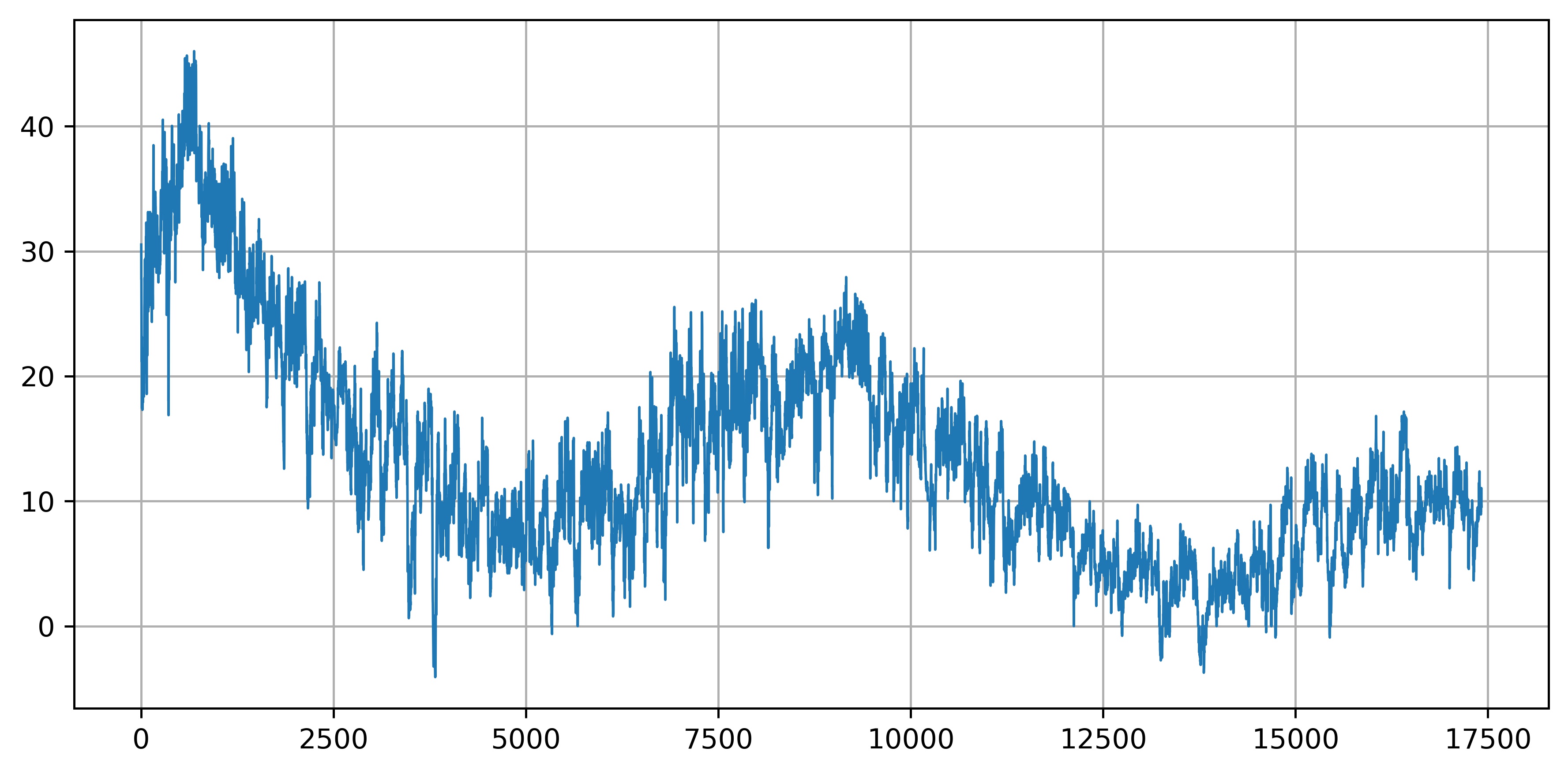
(a) ETTh1

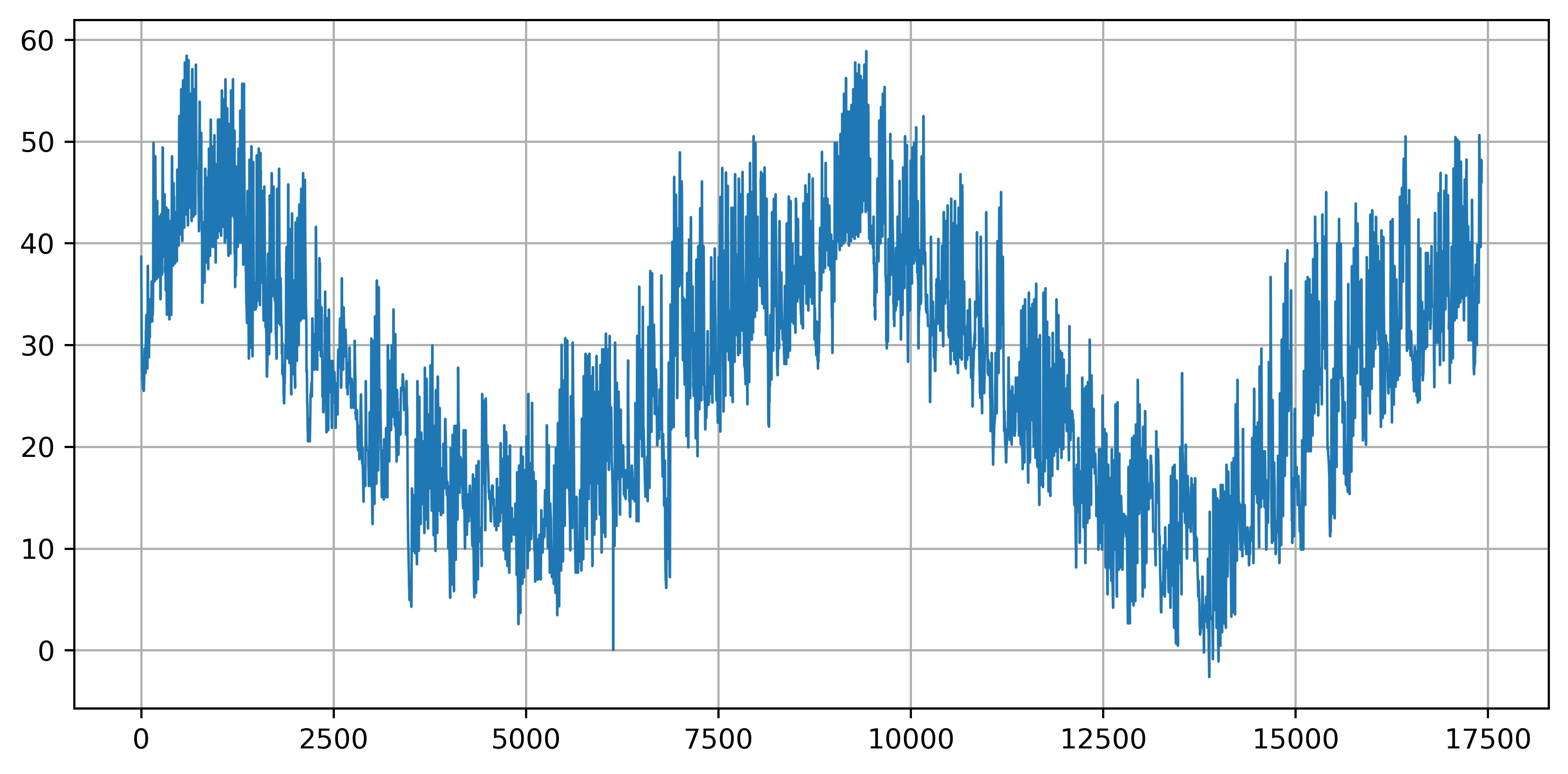
(b) ETTh2

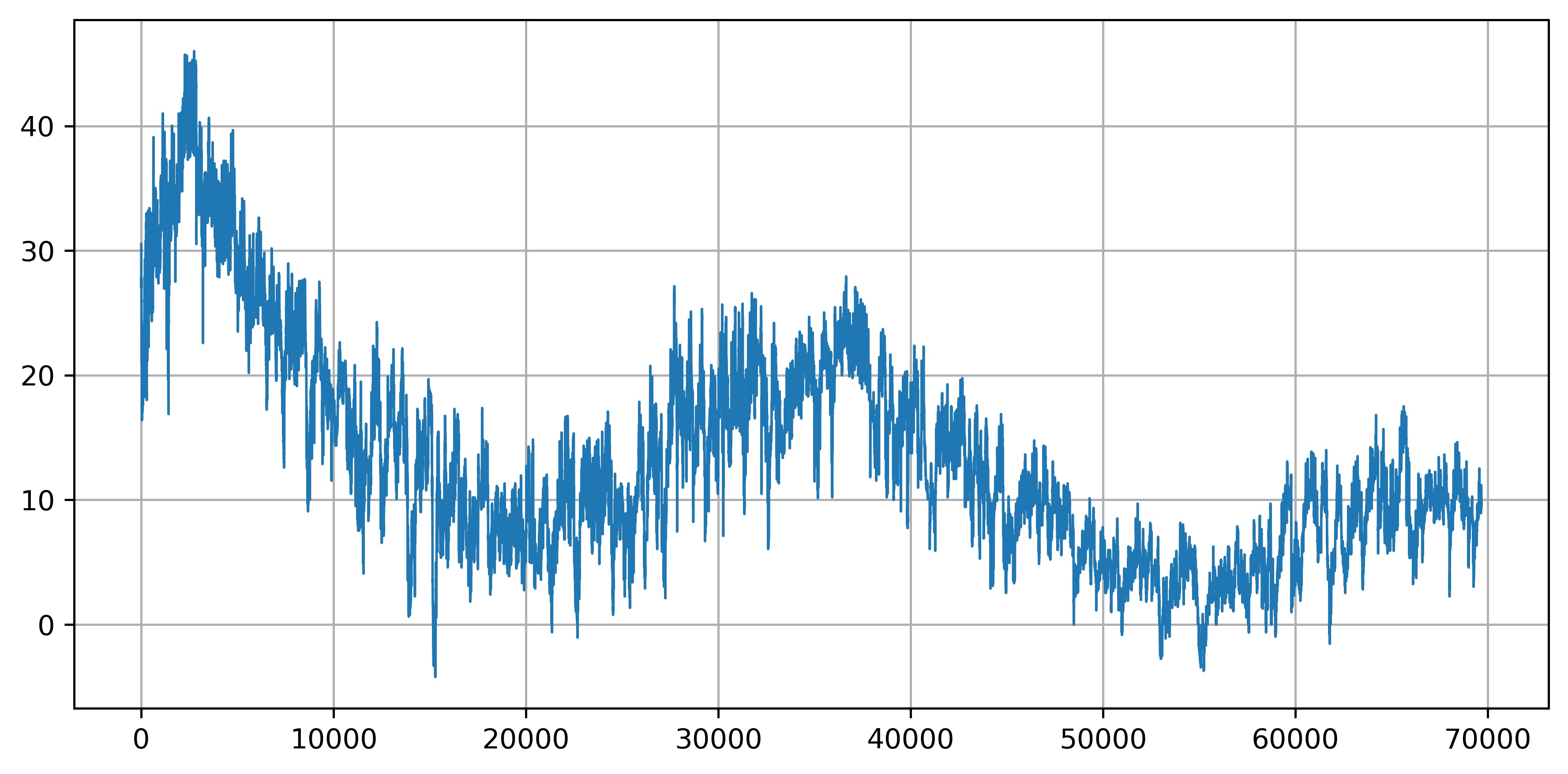
(c) ETTm1

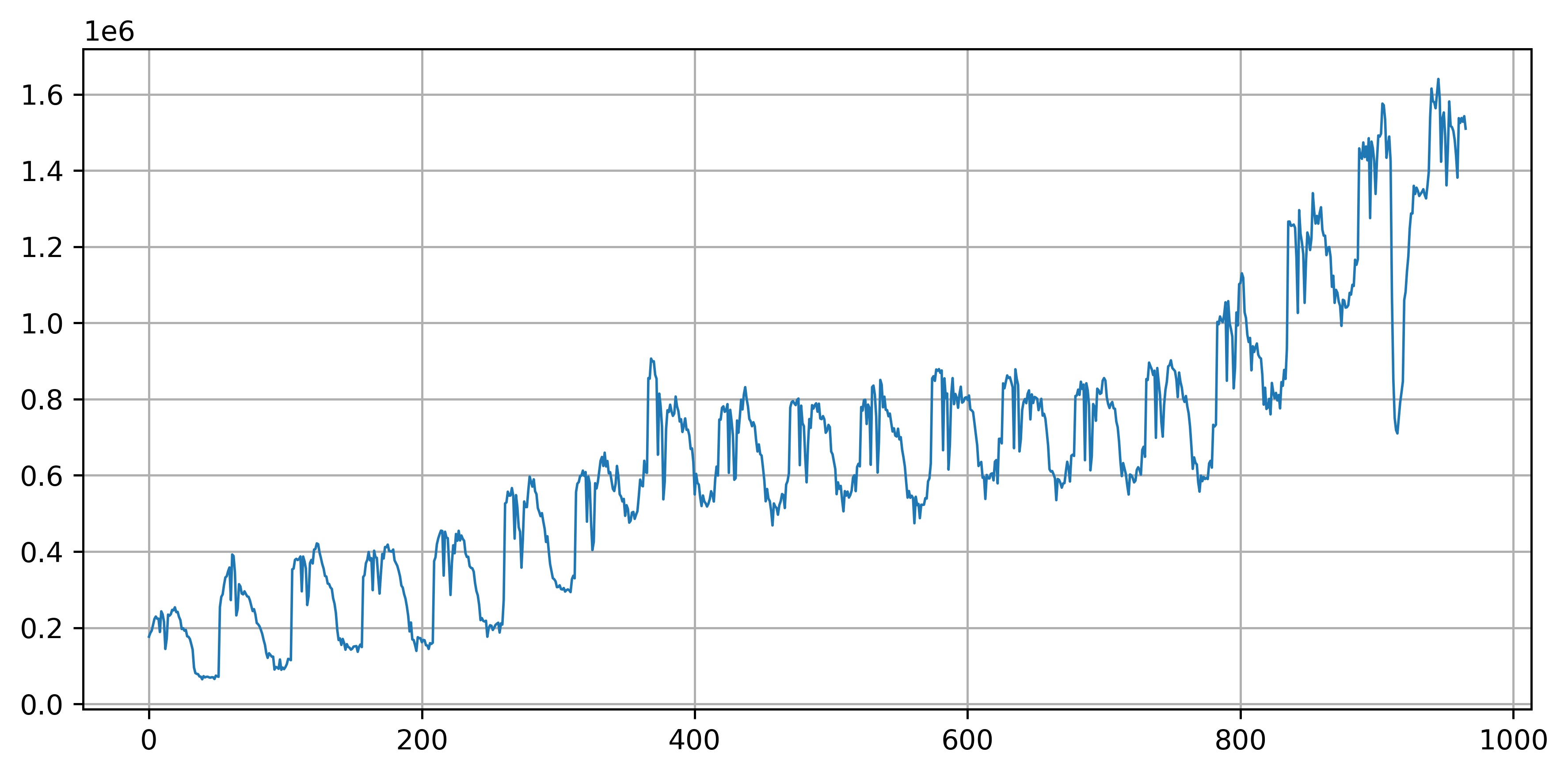
(d) ILI

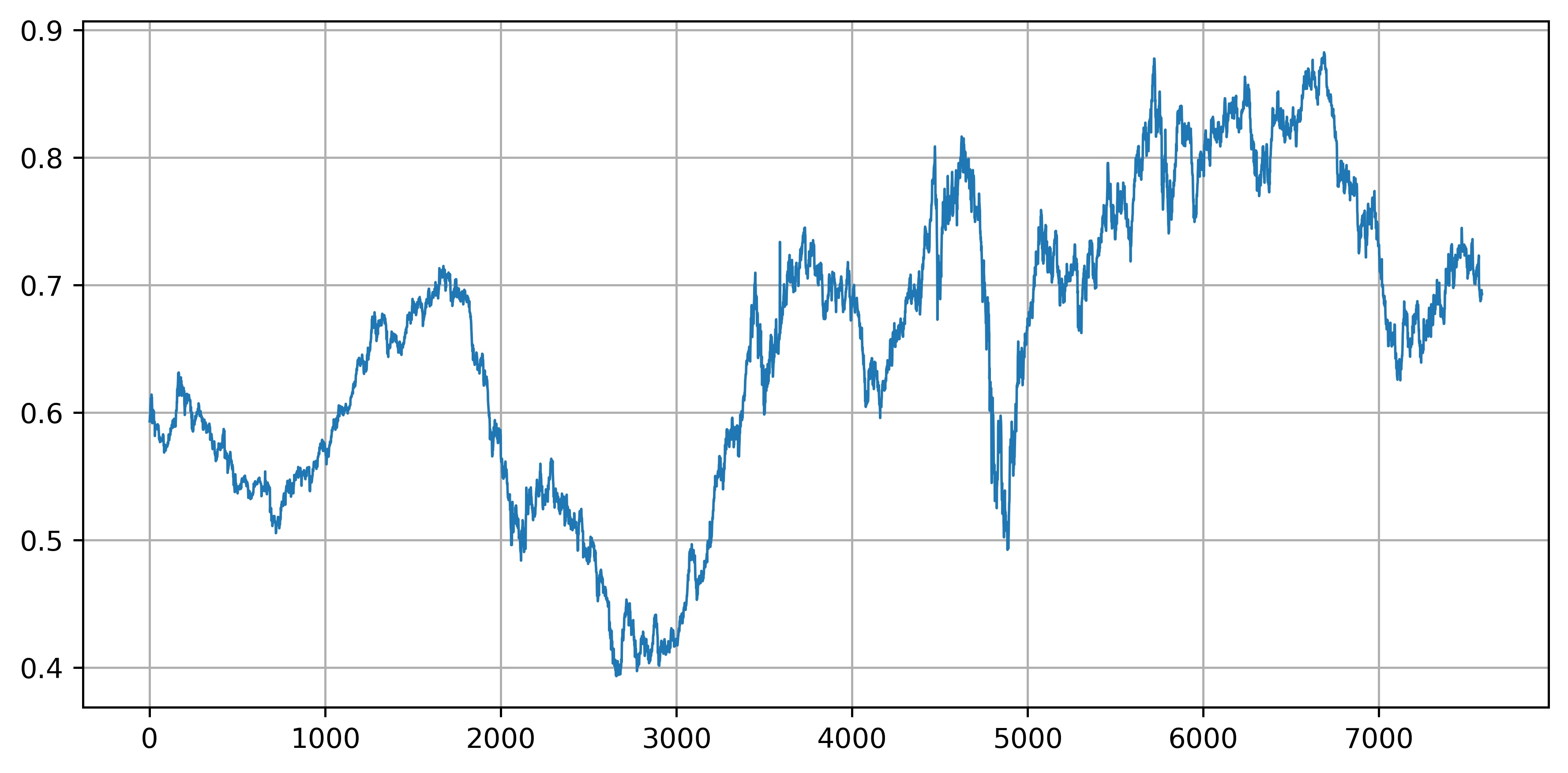
(e) Exchange

Figure 3: A visualization of datasets’ forecasting targets.

4.2 Experimental Setup

Baselines We compared our TSD model with six baseline approaches. Regarding multivariate time series forecasting, we designed the experiments similar to the Autoformer model [59], a standard benchmark for much following-up time series forecasting research. More concretely, we compare TSD with Autoformer [59], Informer [66], LogTrans [20], Reformer [14], LSTNet [17], and LSTM [8]. We reused the experimental reports in the Autoformer paper after randomly double-checking by re-running several experiments not to repeat all implementations on all datasets. Additionally, regarding univariate time series prediction, we designed the experiments similar to the Informer model [66]. Here, we compare our model with Informer, Reformer, LogTrans, DeepAR [42], Yformer [23], and Query Selector [15]. The Git repository is available at .

Hyperparameter Optimization We conduct a grid search over the hyperparameters, and the ranges are given in the following. We set the number of the encoder as one while mainly focusing on the Conv-down-up architecture design, which is the core power of the TSD model. The hidden state sequence $z$ size is selected from $\{512,1024,1280,1536\}$ while the number of heads is $\{8,16,32\}$. The number of up-sampling and down-sampling blocks is $\{3,4,5\}$. The dropout values are searched from $\{0.05,0.1,0.2,0.3\}$. We performed a grid search of the learning rate of $\{0.00001,0.00002,0.000001,0.000005,0.0000001\}$. Furthermore, we apply a scheduling reduction of learning rate by a factor $\gamma$ of $\{0.97,0.95,0.87,0.85\}$ with a step size of $\{2,5,8\}$. The training epoch range is $\{15,20,25,30,35\}$. The number of heads in self-attention is from $\{8,16\}$. Regarding the optimizer, we select AdamW.

Metrics and Implementation Details We trained the TSD model regarding optimizing the mean absolute error $\textrm{MAE}=\frac{1}{n}\sum_{i=1}^{n}|\mathbf{y}-\hat{\mathbf{y}}|$ and mean squared error $\textrm{MSE}=\frac{1}{n}\sum_{i=1}^{n}(\mathbf{y}-\hat{\mathbf{y}})^{2}$ losses on each prediction horizon. We conducted most of Pytorch implementation on high-performance computing nodes equipped with a GeForce RTX 2080Ti 32GB. We ran all experiments three times and reported the average results.

4.3 Results and Analysis

We select datasets under a wide range of horizon lengths from 24 to 720-time points to compare prediction capacity in the challenging multivariate scenario. Regarding the multivariate time series forecasting, Table 1 summarizes the experimental results of all models and benchmarks, while Figure 1 visualizes a relative comparison in trends. As for this experimental scenario, TSD has achieved remarkable performance in all benchmarks and all forecasting horizons. Especially under the optimization for the MSE loss, TSD outperforms six baselines in all 23 different forecasting lengths. Autoformer achieves better results in only 4 MAE cases out of 46 cases in both MSE and MAE. However, these better results fall into short forecasting horizons, e.g., (48, 168) and (96, 192) in ETTh2 and Exchange, respectively. The trends of ETTh1, ETTh2, ILI, and ETTm1 in Figure 1 have proven the consistent prediction power of TSD in far horizons. Especially, under the MSE loss, compared to the previous best state-of-the-art performance, TSD gives average 65% reduction in ETTh1, 29% in ETTh2, 65% in ETTm1, 18% in Exchange, and 56% in ILI. A similar reduction is observed regarding the MAE loss. The error reduction harmonizes with trends and nature of the data as shown in Figure 1. ETTh1 and ETTm1 share a general downward trend, and the data part corresponding to the test set has a small fluctuation amplitude. Contrary to ETTh1 and ETTm1, the ILI dataset tends to increase, and the corresponding test set data has a larger fluctuation amplitude. Due to the unforeseen interaction between countless economic phenomena, the Exchange dataset is comparatively challenging. Therefore, a reduction of 18% is achieved. Overall, 46 reported results in 10 different forecasting horizons, TSD yields a 31% reduction in both MSE and MAE losses. It proves TSD’s superiority against several current best models for many complex real-world multivariate forecasting applications, including early disease warning, long-term financial planning, and resource consumption arrangement.

As for the univariate scenario, i.e $N=1$, TSD has also achieved consistent performance in all benchmarks and all forecasting horizons. TSD yields the best scores in 28 out of 30 experimental cases within five different horizons. Note that TSD has noticeably outperformed DeepAR, the back-bone model for Amazon Forecast Service. The Query Selector model is a robust approach outperforming Informer in all three datasets in both losses. However, compared to our model, the Query Selector is only better in two cases, e.g., ETTm1 at 672 horizons for MSE and MAE. The relative error reduction in both MSE and MAE losses is 46%.

Table 1: Multivariate time series forecasting results. A lower MSE or MAE indicates better forecasting. The best scores are in bold.

Model		TSD		Autoformer		Informer		LogTrans		Reformer		LSTNet		LSTM
Data & Metric		MSE	MAE	MSE	MAE	MSE	MAE	MSE	MAE	MSE	MAE	MSE	MAE	MSE	MAE
ETTh1	24	0.115	0.285	0.384	0.425	0.577	0.549	0.686	0.604	0.991	0.754	1.293	0.901	0.650	0.624
	48	0.119	0.279	0.392	0.419	0.685	0.625	0.766	0.757	1.313	0.906	1.456	0.960	0.702	0.675
	168	0.191	0.313	0.490	0.481	0.931	0.752	1.002	0.846	1.824	1.138	1.997	1.214	1.212	0.867
	336	0.141	0.285	0.505	0.484	1.128	0.873	1.362	0.952	2.117	1.280	2.655	1.369	1.424	0.994
	720	0.233	0.416	0.498	0.500	1.215	0.896	1.397	1.291	2.415	1.520	2.143	1.380	1.960	1.322
ETTh2	24	0.189	0.270	0.261	0.341	0.720	0.665	0.828	0.750	1.531	1.613	2.742	1.457	1.143	0.813
	48	0.242	0.538	0.312	0.373	1.457	1.001	1.806	1.034	1.871	1.735	3.567	1.687	1.671	1.221
	168	0.320	0.493	0.457	0.455	3.489	1.515	4.070	1.681	4.660	1.846	3.242	2.513	4.117	1.674
	336	0.309	0.462	0.471	0.475	2.723	1.340	3.875	1.763	4.028	1.688	2.544	2.591	3.434	1.549
	720	0.314	0.472	0.474	0.484	3.467	1.473	3.913	1.552	5.381	2.015	4.625	3.709	3.963	1.788
ETTm1	24	0.145	0.306	0.383	0.403	0.323	0.369	0.419	0.412	0.724	0.607	1.968	1.170	0.621	0.629
	48	0.143	0.293	0.454	0.453	0.494	0.503	0.507	0.583	1.098	0.777	1.999	1.215	1.392	0.939
	96	0.268	0.390	0.481	0.463	0.678	0.614	0.768	0.792	1.433	0.945	2.762	1.542	1.339	0.913
	288	0.157	0.316	0.634	0.528	1.056	0.786	1.462	1.320	1.820	1.094	1.257	2.076	1.740	1.124
	672	0.149	0.313	0.606	0.542	1.192	0.926	1.669	1.461	2.187	1.232	1.917	2.941	2.736	1.555
Exchange	96	0.184	0.369	0.197	0.323	0.847	0.752	0.968	0.812	1.065	0.829	1.551	1.058	1.453	1.049
	192	0.262	0.445	0.300	0.369	1.204	0.895	1.040	0.851	1.188	0.906	1.477	1.028	1.846	1.179
	336	0.293	0.422	0.509	0.524	1.672	1.036	1.659	1.081	1.357	0.976	1.507	1.031	2.136	1.231
	720	1.307	0.758	1.447	0.941	2.478	1.310	1.941	1.127	1.510	1.016	2.285	1.243	2.984	1.427
ILI	24	1.514	1.103	3.483	1.287	5.764	1.677	4.480	1.444	4.400	1.382	6.026	1.770	5.914	1.734
	36	1.449	1.086	3.103	1.148	4.755	1.467	4.799	1.467	4.783	1.448	5.340	1.668	6.631	1.845
	48	1.186	0.971	2.669	1.085	4.763	1.469	4.800	1.468	4.832	1.465	6.080	1.787	6.736	1.857
	60	1.140	0.946	2.770	1.125	5.264	1.564	5.278	1.560	4.882	1.483	5.548	1.720	6.870	1.879

4.4 Discussions

When applying prediction principles to sequential data, e.g., natural language or time series, contextual information weighs a lot, primarily when long-range dependencies exist. In this context, the issues of gradient vanishing and explosion, model size, and dependencies depend on the length of the sequential data. Transformer’s self-attention approach successfully addressed those mentioned issues by designing a novel encoder-decoder architecture [54]. Developed upon that architecture, the Probsparse self-attention was introduced to overcome the memory bottleneck of the transformer while acceptably handling extremely long input sequences. Table 4 presents the evolutional simplification of general encoder-decoder pairs throughout the research. Employing model design, the complexity of an encoder-decoder architecture is significantly reduced. For instance, the number of encoders and decoders in the Informer model was reduced from 6 to 4 and 6 to 2, respectively. However, the long-term forecasting problem of time series remains challenging, although various self-attention mechanisms were adopted. In far-horizon forecasting, a model, instead of attending to several single points, treat sub-series level and aggregates dependencies discovery and representation. Consequently, the auto-correlation mechanism was developed [59], which yielded a 38% relative improvement on compared models. The number of encoders and decoders was noticeably reduced from 4 to 2 and 2 to 1, respectively. One point to note is that the authors of those mentioned models do not provide any ablation study on why they chose the number of encoders and decoders. However, the core idea is to balance forecasting accuracy and computation efficiency. As discussed in Section 1, our hypothesis is to automatically encode the correct temporal pattern to the suitable self-attention heads and to learn saliency patterns emerging from the sequential data. Hence, one encoder is enough to output a self-attention representation. Unlike the existing methods, we completely replace a general decoder with a U-sharp architecture, effectively addressing the image segmentation task. Generally speaking, we also want to segment time series in automatic processing and discovery.

Table 2: Univariate time series forecasting results. A lower MSE or MAE indicates better forecasting. The best scores are in bold.

Models		TSD		Informer		Reformer		LogTrans		DeepAR		Yformer		Query Selector
Dataset & Metric		MSE	MAE	MSE	MAE	MSE	MAE	MSE	MAE	MSE	MAE	MSE	MAE	MSE	MAE
ETTh1	24	0.018	0.102	0.098	0.247	0.222	0.389	0.103	0.259	0.107	0.280	0.082	0.230	0.043	0.161
	48	0.043	0.166	0.158	0.319	0.284	0.445	0.167	0.328	0.162	0.327	0.139	0.308	0.072	0.211
	168	0.082	0.225	0.183	0.346	1.522	1.191	0.207	0.375	0.239	0.422	0.111	0.268	0.093	0.237
	336	0.094	0.237	0.222	0.387	1.860	1.124	0.230	0.398	0.445	0.552	0.195	0.365	0.126	0.284
	720	0.129	0.291	0.269	0.435	2.112	1.436	0.273	0.463	0.658	0.707	0.226	0.394	0.213	0.373
ETTm1	24	0.011	0.082	0.030	0.137	0.095	0.228	0.065	0.202	0.091	0.243	0.024	0.118	0.013	0.087
	48	0.019	0.110	0.069	0.203	0.249	0.390	0.078	0.220	0.219	0.362	0.048	0.173	0.034	0.140
	96	0.038	0.161	0.194	0.372	0.920	0.767	0.199	0.386	0.364	0.496	0.143	0.311	0.070	0.210
	288	0.057	0.199	0.401	0.554	1.108	1.245	0.411	0.572	0.948	0.795	0.150	0.316	0.154	0.324
	672	0.341	1.052	0.512	0.644	1.793	1.528	0.598	0.702	2.437	1.352	0.305	0.476	0.173	0.342
ETTh2	24	0.075	0.210	0.093	0.240	0.263	0.437	0.102	0.255	0.098	0.263	0.082	0.221	0.084	0.223
	48	0.073	0.213	0.155	0.314	0.458	0.545	0.169	0.348	0.163	0.341	0.139	0.334	0.111	0.262
	168	0.110	0.270	0.232	0.389	1.029	0.879	0.246	0.422	0.255	0.414	0.111	0.337	0.175	0.332
	336	0.121	0.273	0.263	0.417	1.668	1.228	0.267	0.437	0.604	0.607	0.195	0.391	0.208	0.371
	720	0.123	0.273	0.277	0.431	2.030	1.721	0.303	0.493	0.429	0.580	0.226	0.382	0.258	0.413

5 Ablation Study

5.1 Pooling Selection

TSD comprises $u$-pair blocks of down-sampling and up-sampling that play a central role in current architecture. At each block $l$, we propose to use a pooling layer with a kernel size of $k_{l}=3$ to help the layer focus a specific scale if its input. It helps reduce the input’s width, release memory usage, reduce learnable parameters, alleviate the effects of overfitting, and limit the computation. We carefully explore max and average pooling operations and the model’s stability under various far-horizon. Table 3 presents the empirical evaluation of pooling configurations. This ablation shows that max pooling is more stable in long-term forecasting, e.g., from a horizon of 60 and beyond. We have randomly tested on other datasets and observed a similar trend, more details can be founded in supplementary materials.

Table 3: Empirical evaluation of eight different horizons with two pooling settings. The best scores are in bold.

Data	Horizon	MaxPool		AveragePool
		MSE	MAE	MSE	MAE
ILI	24	1.514	1.103	1.577	1.108
	36	1.449	1.086	1.429	1.042
	48	1.186	0.971	1.239	0.962
	60	1.140	0.946	1.146	0.947
Exchange	96	0.184	0.369	0.985	1.263
	192	0.262	0.445	0.347	0.453
	336	0.293	0.422	0.455	0.513
	720	1.307	0.758	1.620	1.787

Table 4: The simplification of models’ architecture and its reason. Referring to Attention, we mean the model developed by  [54].

Model	# encoder	# decoder	Reason of simplification
Attention	6	6	Replacement of recurrent layers with encoder-decoder pairs
Informer	4	2	Introduction of Probsparse self-attention
Autoformer	2	1	Introduction of auto-correlation mechanism
Our model	1	1	Introduction of saliency detection mechanism

5.2 Architecture Variations

In this ablation, we test several variations of TSD architecture and its performance in three alternative layouts: $\{3,4,5\}$ conv-down-up blocks. We believe that the advantages of TSD architecture are rooted in its flexibility in multi-block design for a specific dataset. Table 5 compares TSD alternatives qualitatively. All hyperparameters are the same, excluding the block design. Most importantly, the best model design is to have a balance between forecasting accuracy and computation costs. Therefore, in this paper, we chose a TSD architecture with four conv-down-up blocks for all experiments.

Table 5: Evaluation of architectural variations of our proposed model. The best scores are in bold.

Model	Horizon	3 conv-down-up blocks		4 conv-down-up blocks		5 conv-down-up blocks
		MSE	MAE	MSE	MAE	MSE	MAE
ILI	24	1.519	1.081	1.514	1.103	1.537	1.107
	36	1.396	1.080	1.449	1.086	1.405	1.128
	48	1.224	0.958	1.186	0.971	1.278	0.978
	60	1.126	0.924	1.140	0.946	1.125	0.930
Exchange	96	0.643	1.442	0.184	0.369	3.109	1.406
	192	1.818	1.676	0.262	0.445	0.287	0.458
	336	0.934	1.343	0.293	0.422	0.463	0.494
	720	1.411	0.937	1.307	0.758	1.505	1.040

6 Future Work

Although the concept of TSD demonstrates remarkable experimental outcomes, it requires a thorough hyperparameter search, as outlined in Section 4.2. The pre-defined range of hyperparameters heavily relies on domain expertise provided by an expert in the field. Specifically, the investigation involves determining the appropriate layer size in the convolutional blocks, establishing the optimal sequence of layers and examining its impact on prediction, and exploring potential interactions between the number of heads and conv-down-up blocks. This process entails over 700 manual trial-and-error iterations in selecting the hyperparameter ranges, further enhancing performance. We acknowledge that hyperparameter optimization remains a limitation of the model.

While U-Net architectures are predominantly employed in biomedical image segmentation to automate identifying and detecting target regions or sub-regions, our study demonstrates that TSD can be effectively utilized for time series data. It is essential to highlight that a thorough analysis of U-Net variants [46, 35], encompassing inter-modality and intra-modality categorization, holds significance in gaining deeper insights into the challenges associated with time series forecasting and saliency detection. This analysis recommends a valuable avenue for future research endeavors in this field.

This study scrutinizes the efficacy of automatically encoding saliency-related temporal patterns by establishing connections with appropriate attention heads by incorporating information contracting and expanding blocks inspired by the U-Net style architecture. To substantiate our claims, we utilize an embarrassingly simple TSD forecasting baseline. It is crucial to note that the contributions of this work do not solely lie in proposing a state-of-the-art model; instead, they stem from posing a significant question, presenting surprising comparisons, and elucidating the effectiveness of TSD, as asserted in existing literature, from various perspectives. Our comprehensive investigations will prove advantageous for future research endeavors in this domain. The initial TSD model exhibits limited capacity, and its primary purpose is to serve as a straightforward yet competitive baseline with robust interpretability for subsequent research. TSD sets a new baseline for all pursuing multi-discipline work on popular time series benchmarks.

7 Conclusion

This research introduces an effective time series forecasting model called Temporal Saliency Detection, inspired by advancements in machine translation and down-and-up samplings in the context of image segmentation tasks. The proposed TSD model leverages the U-Net architecture and demonstrates superior predictability compared to existing models. This work’s fundamental premise is the need for a technique to encode saliency-related temporal patterns through appropriate attention head connections automatically. The outcomes of our study underscore the significance of automatically learning saliency patterns from time series data, as the proposed TSD model significantly outperforms several state-of-the-art approaches and benchmark methods. In the multivariate scenario, our experiments reveal that TSD achieves a remarkable 31% reduction in MSE and MAE losses across 46 reported results encompassing ten diverse forecasting horizons. Similarly, in the univariate forecasting setting, TSD yields a noteworthy 46% reduction in both MSE and MAE losses. The authors conducted an ablation analysis to ensure the proposed model’s effectiveness and expected behavior. However, it is worth noting that further potential for improvement is evident, suggesting the need for hyperparameter optimization and the exploitation of U-net variants. These findings underscore the efficacy and promise of the TSD model in the context of time series forecasting while also highlighting avenues for future research and refinement.

References

- [1] Ariyo, A.A., Adewumi, A.O., Ayo, C.K.: Stock price prediction using the arima model. In: 2014 UKSim-AMSS 16th International Conference on Computer Modelling and Simulation. pp. 106–112. IEEE (2014)
- [2] Bahdanau, D., Cho, K., Bengio, Y.: Neural machine translation by jointly learning to align and translate. arXiv preprint arXiv:1409.0473 (2014)
- [3] Challu, C., Olivares, K.G., Oreshkin, B.N., Garza, F., Mergenthaler, M., Dubrawski, A.: N-hits: Neural hierarchical interpolation for time series forecasting. arXiv preprint arXiv:2201.12886 (2022)
- [4] Duarte, F.S., Rios, R.A., Hruschka, E.R., de Mello, R.F.: Decomposing time series into deterministic and stochastic influences: A survey. Digital Signal Processing 95, 102582 (2019)
- [5] Fan, C., Zhang, Y., Pan, Y., Li, X., Zhang, C., Yuan, R., Wu, D., Wang, W., Pei, J., Huang, H.: Multi-horizon time series forecasting with temporal attention learning. In: Proceedings of the 25th ACM SIGKDD International conference on knowledge discovery & data mining. pp. 2527–2535 (2019)
- [6] Gao, C., Zhang, N., Li, Y., Bian, F., Wan, H.: Self-attention-based time-variant neural networks for multi-step time series forecasting. Neural Computing and Applications 34(11), 8737–8754 (2022)
- [7] Hewamalage, H., Bergmeir, C., Bandara, K.: Recurrent neural networks for time series forecasting: Current status and future directions. International Journal of Forecasting 37(1), 388–427 (2021)
- [8] Hochreiter, S., Schmidhuber, J.: Long short-term memory. Neural computation 9(8), 1735–1780 (1997)
- [9] Hu, B., Tunison, P., RichardWebster, B., Hoogs, A.: Xaitk-saliency: An open source explainable ai toolkit for saliency. In: Proceedings of the AAAI Conference on Artificial Intelligence. vol. 37, pp. 15760–15766 (2023)
- [10] Ibtehaz, N., Rahman, M.S.: Multiresunet: Rethinking the u-net architecture for multimodal biomedical image segmentation. Neural networks 121, 74–87 (2020)
- [11] Ismail, A.A., Corrada Bravo, H., Feizi, S.: Improving deep learning interpretability by saliency guided training. In: Ranzato, M., Beygelzimer, A., Dauphin, Y., Liang, P., Vaughan, J.W. (eds.) Advances in Neural Information Processing Systems. vol. 34, pp. 26726–26739. Curran Associates, Inc. (2021)
- [12] Ismail, A.A., Gunady, M., Bravo, H.C., Feizi, S.: Benchmarking deep learning interpretability in time series predictions. In: Proceedings of the 34th International Conference on Neural Information Processing Systems. NIPS’20, Curran Associates Inc., Red Hook, NY, USA (2020)
- [13] Jin, X., Park, Y., Maddix, D., Wang, H., Wang, Y.: Domain adaptation for time series forecasting via attention sharing. In: International Conference on Machine Learning. pp. 10280–10297. PMLR (2022)
- [14] Kitaev, N., Kaiser, Ł., Levskaya, A.: Reformer: The efficient transformer. arXiv preprint arXiv:2001.04451 (2020)
- [15] Klimek, J., Klimek, J., Kraskiewicz, W., Topolewski, M.: Long-term series forecasting with query selector–efficient model of sparse attention. arXiv preprint arXiv:2107.08687 (2021)
- [16] Kohl, S., Romera-Paredes, B., Meyer, C., De Fauw, J., Ledsam, J.R., Maier-Hein, K., Eslami, S., Jimenez Rezende, D., Ronneberger, O.: A probabilistic u-net for segmentation of ambiguous images. Advances in neural information processing systems 31 (2018)
- [17] Lai, G., Chang, W.C., Yang, Y., Liu, H.: Modeling long-and short-term temporal patterns with deep neural networks. In: The 41st International ACM SIGIR Conference on Research & Development in Information Retrieval. pp. 95–104 (2018)
- [18] Lara-Benítez, P., Carranza-García, M., Riquelme, J.C.: An experimental review on deep learning architectures for time series forecasting. International Journal of Neural Systems 31(03), 2130001 (2021)
- [19] Li, H., Chen, G., Li, G., Yu, Y.: Motion guided attention for video salient object detection. In: Proceedings of the IEEE/CVF international conference on computer vision. pp. 7274–7283 (2019)
- [20] Li, S., Jin, X., Xuan, Y., Zhou, X., Chen, W., Wang, Y.X., Yan, X.: Enhancing the locality and breaking the memory bottleneck of transformer on time series forecasting. Advances in Neural Information Processing Systems 32, 5243–5253 (2019)
- [21] Lim, B., Arık, S.Ö., Loeff, N., Pfister, T.: Temporal fusion transformers for interpretable multi-horizon time series forecasting. International Journal of Forecasting (2021)
- [22] Ma, J., Shou, Z., Zareian, A., Mansour, H., Vetro, A., Chang, S.F.: Cdsa: cross-dimensional self-attention for multivariate, geo-tagged time series imputation. arXiv preprint arXiv:1905.09904 (2019)
- [23] Madhusudhanan, K., Burchert, J., Duong-Trung, N., Born, S., Schmidt-Thieme, L.: Yformer: U-net inspired transformer architecture for far horizon time series forecasting. arXiv preprint arXiv:2110.08255 (2021)
- [24] Makridakis, S., Spiliotis, E., Assimakopoulos, V.: Predicting/hypothesizing the findings of the m5 competition. International Journal of Forecasting (2021)
- [25] Masini, R.P., Medeiros, M.C., Mendes, E.F.: Machine learning advances for time series forecasting. Journal of Economic Surveys (2021)
- [26] Meisenbacher, S., Turowski, M., Phipps, K., Rätz, M., Müller, D., Hagenmeyer, V., Mikut, R.: Review of automated time series forecasting pipelines. Wiley Interdisciplinary Reviews: Data Mining and Knowledge Discovery p. e1475 (2022)
- [27] Morrison, K., Mehra, A., Perer, A.: Shared interest… sometimes: Understanding the alignment between human perception, vision architectures, and saliency map techniques. In: Proceedings of the IEEE/CVF Conference on Computer Vision and Pattern Recognition. pp. 3775–3780 (2023)
- [28] Olivares, K.G., Meetei, N., Ma, R., Reddy, R., Cao, M.: Probabilistic hierarchical forecasting with deep poisson mixtures. In: NeurIPS 2021 Workshop on Deep Generative Models and Downstream Applications (2021)
- [29] Oreshkin, B.N., Carpov, D., Chapados, N., Bengio, Y.: N-beats: Neural basis expansion analysis for interpretable time series forecasting. arXiv preprint arXiv:1905.10437 (2019)
- [30] Pan, Q., Hu, W., Chen, N.: Two birds with one stone: Series saliency for accurate and interpretable multivariate time series forecasting. In: Zhou, Z.H. (ed.) Proceedings of the Thirtieth International Joint Conference on Artificial Intelligence, IJCAI-21. pp. 2884–2891. International Joint Conferences on Artificial Intelligence Organization (8 2021)
- [31] Pan, Q., Hu, W., Chen, N.: Two birds with one stone: Series saliency for accurate and interpretable multivariate time series forecasting. In: IJCAI. pp. 2884–2891 (2021)
- [32] Parvatharaju, P.S., Doddaiah, R., Hartvigsen, T., Rundensteiner, E.A.: Learning saliency maps to explain deep time series classifiers. In: Proceedings of the 30th ACM International Conference on Information & Knowledge Management. pp. 1406–1415 (2021)
- [33] Perslev, M., Jensen, M., Darkner, S., Jennum, P.J., Igel, C.: U-time: A fully convolutional network for time series segmentation applied to sleep staging. Advances in Neural Information Processing Systems 32, 4415–4426 (2019)
- [34] Piccialli, F., Giampaolo, F., Prezioso, E., Camacho, D., Acampora, G.: Artificial intelligence and healthcare: Forecasting of medical bookings through multi-source time-series fusion. Information Fusion 74, 1–16 (2021)
- [35] Punn, N.S., Agarwal, S.: Modality specific u-net variants for biomedical image segmentation: a survey. Artificial Intelligence Review 55(7), 5845–5889 (2022)
- [36] Qin, Y., Song, D., Chen, H., Cheng, W., Jiang, G., Cottrell, G.W.: A dual-stage attention-based recurrent neural network for time series prediction. In: IJCAI (2017)
- [37] Rangapuram, S.S., Seeger, M.W., Gasthaus, J., Stella, L., Wang, Y., Januschowski, T.: Deep state space models for time series forecasting. Advances in neural information processing systems 31 (2018)
- [38] Rombach, R., Blattmann, A., Lorenz, D., Esser, P., Ommer, B.: High-resolution image synthesis with latent diffusion models. CoRR abs/2112.10752 (2021)
- [39] Ronneberger, O., Fischer, P., Brox, T.: U-net: Convolutional networks for biomedical image segmentation. In: International Conference on Medical image computing and computer-assisted intervention. pp. 234–241. Springer (2015)
- [40] Saadallah, A., Jakobs, M., Morik, K.: Explainable online deep neural network selection using adaptive saliency maps for time series forecasting. In: Machine Learning and Knowledge Discovery in Databases. Research Track: European Conference, ECML PKDD 2021, Bilbao, Spain, September 13–17, 2021, Proceedings, Part I. pp. 404–420. Springer (2021)
- [41] Saadallah, A., Jakobs, M., Morik, K.: Explainable online ensemble of deep neural network pruning for time series forecasting. Machine Learning 111(9), 3459–3487 (2022)
- [42] Salinas, D., Flunkert, V., Gasthaus, J., Januschowski, T.: Deepar: Probabilistic forecasting with autoregressive recurrent networks. International Journal of Forecasting 36(3), 1181–1191 (2020)
- [43] Sartirana, D., Rotiroti, M., Bonomi, T., De Amicis, M., Nava, V., Fumagalli, L., Zanotti, C.: Data-driven decision management of urban underground infrastructure through groundwater-level time-series cluster analysis: the case of milan (italy). Hydrogeology Journal pp. 1–21 (2022)
- [44] Sezer, O.B., Gudelek, M.U., Ozbayoglu, A.M.: Financial time series forecasting with deep learning: A systematic literature review: 2005–2019. Applied Soft Computing 90, 106181 (2020)
- [45] Shih, S.Y., Sun, F.K., Lee, H.y.: Temporal pattern attention for multivariate time series forecasting. Machine Learning 108(8), 1421–1441 (2019)
- [46] Siddique, N., Paheding, S., Elkin, C.P., Devabhaktuni, V.: U-net and its variants for medical image segmentation: A review of theory and applications. Ieee Access 9, 82031–82057 (2021)
- [47] Song, H., Rajan, D., Thiagarajan, J.J., Spanias, A.: Attend and diagnose: Clinical time series analysis using attention models. In: Thirty-second AAAI conference on artificial intelligence (2018)
- [48] Stefenon, S.F., Ribeiro, M.H.D.M., Nied, A., Yow, K.C., Mariani, V.C., dos Santos Coelho, L., Seman, L.O.: Time series forecasting using ensemble learning methods for emergency prevention in hydroelectric power plants with dam. Electric Power Systems Research 202, 107584 (2021)
- [49] Stoller, D., Tian, M., Ewert, S., Dixon, S.: Seq-u-net: A one-dimensional causal u-net for efficient sequence modelling. In: Bessiere, C. (ed.) Proceedings of the Twenty-Ninth International Joint Conference on Artificial Intelligence, IJCAI-20. pp. 2893–2900. International Joint Conferences on Artificial Intelligence Organization (7 2020)
- [50] Taylor, S.J., Letham, B.: Forecasting at scale. The American Statistician 72(1), 37–45 (2018)
- [51] Tealab, A.: Time series forecasting using artificial neural networks methodologies: A systematic review. Future Computing and Informatics Journal 3(2), 334–340 (2018)
- [52] Tomar, S., Tirupathi, S., Salwala, D.V., Dusparic, I., Daly, E.: Prequential model selection for time series forecasting based on saliency maps. In: 2022 IEEE International Conference on Big Data (Big Data). pp. 3383–3392. IEEE (2022)
- [53] Ullah, I., Jian, M., Hussain, S., Guo, J., Yu, H., Wang, X., Yin, Y.: A brief survey of visual saliency detection. Multimedia Tools and Applications 79(45), 34605–34645 (2020)
- [54] Vaswani, A., Shazeer, N., Parmar, N., Uszkoreit, J., Jones, L., Gomez, A.N., Kaiser, Ł., Polosukhin, I.: Attention is all you need. In: Advances in neural information processing systems. pp. 5998–6008 (2017)
- [55] Wang, H., Cao, P., Wang, J., Zaïane, O.R.: Uctransnet: Rethinking the skip connections in u-net from a channel-wise perspective with transformer. In: Thirty-Sixth AAAI Conference on Artificial Intelligence, AAAI 2022, Thirty-Fourth Conference on Innovative Applications of Artificial Intelligence, IAAI 2022, The Twelveth Symposium on Educational Advances in Artificial Intelligence, EAAI 2022 Virtual Event, February 22 - March 1, 2022. pp. 2441–2449. AAAI Press (2022)
- [56] Wang, K., Li, K., Zhou, L., Hu, Y., Cheng, Z., Liu, J., Chen, C.: Multiple convolutional neural networks for multivariate time series prediction. Neurocomputing 360, 107–119 (2019)
- [57] Wang, S., Li, B.Z., Khabsa, M., Fang, H., Ma, H.: Linformer: Self-attention with linear complexity. arXiv preprint arXiv:2006.04768 (2020)
- [58] Wen, R., Torkkola, K., Narayanaswamy, B., Madeka, D.: A multi-horizon quantile recurrent forecaster. arXiv preprint arXiv:1711.11053 (2017)
- [59] Xu, J., Wang, J., Long, M., et al.: Autoformer: Decomposition transformers with auto-correlation for long-term series forecasting. Advances in Neural Information Processing Systems 34 (2021)
- [60] Yang, Y., Fan, C., Xiong, H.: A novel general-purpose hybrid model for time series forecasting. Applied Intelligence pp. 1–12 (2021)
- [61] Yu, R., Zheng, S., Anandkumar, A., Yue, Y.: Long-term forecasting using tensor-train rnns. Arxiv (2017)
- [62] Yun, H., Lee, S., Kim, G.: Panoramic vision transformer for saliency detection in 360∘ videos. In: European Conference on Computer Vision. pp. 422–439. Springer (2022)
- [63] Zeng, A., Chen, M., Zhang, L., Xu, Q.: Are transformers effective for time series forecasting? In: Proceedings of the AAAI conference on artificial intelligence. vol. 37, pp. 11121–11128 (2023)
- [64] Zeng, S., Graf, F., Hofer, C., Kwitt, R.: Topological attention for time series forecasting. Advances in Neural Information Processing Systems 34, 24871–24882 (2021)
- [65] Zhang, D., Fu, H., Han, J., Borji, A., Li, X.: A review of co-saliency detection algorithms: fundamentals, applications, and challenges. ACM Transactions on Intelligent Systems and Technology (TIST) 9(4), 1–31 (2018)
- [66] Zhou, H., Zhang, S., Peng, J., Zhang, S., Li, J., Xiong, H., Zhang, W.: Informer: Beyond efficient transformer for long sequence time-series forecasting. In: Proceedings of AAAI (2021)