SAIF: Sparse Adversarial and Imperceptible Attack Framework

Abstract

Adversarial attacks hamper the decision-making ability of neural networks by perturbing the input signal. The addition of calculated small distortion to images, for instance, can deceive a well-trained image classification network. In this work, we propose a novel attack technique called Sparse Adversarial and Imperceptible Attack Framework (SAIF). Specifically, we design imperceptible attacks that contain low-magnitude perturbations at a small number of pixels and leverage these sparse attacks to reveal the vulnerability of classifiers. We use the Frank-Wolfe (conditional gradient) algorithm to simultaneously optimize the attack perturbations for bounded magnitude and sparsity with $O(1/\sqrt{T})$ convergence. Empirical results show that SAIF computes highly imperceptible and interpretable adversarial examples, and largely outperforms state-of-the-art sparse attack methods on ImageNet and CIFAR-10.

1 Introduction

Deep neural networks (DNNs) are widely utilized for various tasks such as object detection [31, 16], classification [23, 18], and anomaly detection [5]. These DNNs are ubiquitously integrated into real-world systems for medical diagnosis, autonomous driving, surveillance, etc., where misguided decision-making can have catastrophic consequences. Therefore, it is crucial to inspect the limitations of DNNs before deployment in such safety-critical systems.

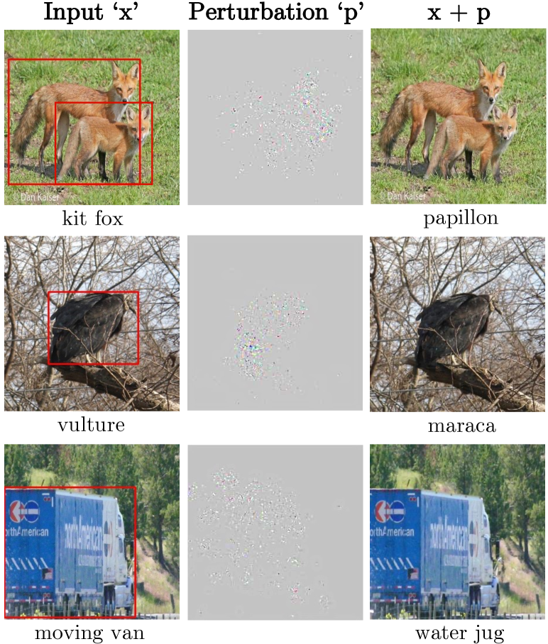
Figure 1: Using the Frank-Wolfe algorithm to jointly constrain the perturbation magnitude and sparsity, we craft an adversarial attack that is very sparse and highly imperceptible. By restricting attack sparsity, we can visualize the most vulnerable pixels in an image. The GT bounding boxes for the subject of the input $\mathbf{x}$ are drawn in red. Note that SAIF mostly distorts pixels within that region. Inception-v3 is used for predicting labels.

Adversarial attacks [34] are one means of exposing the fragility of DNNs. In the classification task, these attacks can fool well-trained classifiers to make arbitrary (untargeted) [28] or targeted misclassifications [4] by negligibly manipulating the input signal. For instance, a road sign classifier can be led to interpret a slightly modified stop sign as a speed limit sign [1]. Such adversarial attacks fool learning algorithms with high confidence while being imperceptible to the human eye. Most attack methods achieve this by constraining the pixel-wise magnitude of the perturbation. Minimizing the number of modified pixels is another strategy for making the perturbations unnoticeable [33, 29]. Bringing these two together generates high-stealth attacks [27, 9, 11, 12, 38].

Existing methods, however, fail to produce attacks with simultaneously very high sparsity and low magnitude perturbations. In this paper, we address this limitation by designing a novel method that produces strong adversarial attacks with a significantly low perturbation strength and high sparsity. Our proposed approach, we call Sparse Adversarial and Imperceptible attack Framework (SAIF), minimally modifies only a fraction of pixels to generate highly concealed adversarial attacks.

SAIF aims to jointly minimize the perturbation magnitude and sparsity. We formulate this objective as a constrained optimization problem. Previous works propose projection-based methods (such as PGD [26]) to optimize similar objectives, however, these require a projection step at each iteration to obtain feasible solutions [9]. Such projections give rise to iterates very close to/at the constraint boundary, and projecting the solutions can diminish their ‘optimality’. Optimization methods such as ADMM [39, 12] and homotopy [12] have also been explored, but have prohibitively long running times for large images.

To address these limitations, we propose to leverage the Frank-Wolfe algorithm (FW) [13] to optimize our objective. FW is a projection-free, iterative method for solving constrained convex optimization problems using conditional gradients. In contrast to PGD attacks, the absence of a projection step allows FW to find perturbations well within the constraint boundaries. Throughout optimization, the iterates are within the constraint limits since they are convex combinations of feasible points. Moreover, there are several algorithmic variants of FW for efficient optimization.

Furthermore, the benefit from adversarial examples can be maximized by examining the vulnerabilities of deep networks alongside model explanations [20, 37, 39]. Magnitude-constrained attacks distort all image pixels, leaving little room to interpret the additive perturbations. Our proposed attack offers explicit control over distortion magnitude and sparsity. This facilitates more controlled and straightforward semantic analyses, such as identifying the top-‘$k$’ pixels that are critical for fooling DNNs.

Concretely, the contributions of this paper are:

• We introduce a novel optimization-based adversarial attack that is visually imperceptible due to low-magnitude distortions to a fraction of image pixels.

• We show through comprehensive experiments that, for tight sparsity and magnitude constraints, SAIF outperforms state-of-the-art sparse attacks by a large margin (by $\geq 2\times$ higher fooling rates for most thresholds).

• Our sparse attack provides transparency by indicating vulnerable pixels. We quantitatively evaluate the overlap between perturbations and salient image regions to emphasize the utility of SAIF for such analyses.

2 Related Works

Magnitude-Constrained Adversarial Attacks.

The first discovered adversarial attack by [34] uses box-constrained L-BFGS to minimize the $\ell_{2}$ norm of additive distortion, however, it is slow and does not scale to larger inputs. To overcome speed limitations, the Fast Gradient Sign Method (FGSM) [17] uses $\ell_{\infty}$ constrained gradient ascent w.r.t. the loss gradient for each pixel, to compute an efficient attack but with poor convergence. Projected Gradient Descent (PGD) is another optimization-based attack algorithm that is fast and computationally cheap, but yields solutions closer to the boundary and often fails to converge [26]. Auto-attack [10] addresses the convergence limitations of PGD. Nevertheless, these attacks distort all the image pixels, potentially leading to high visual perceptibility. We address this shortcoming by explicitly constraining the sparsity of the adversarial perturbations.

Sparsity-Constrained Adversarial Attacks.

The Jacobian-based Saliency Map Attack (JSMA) denotes pixel-wise saliency by backpropagated gradient magnitudes, then searches over the most salient pixels for a sparse targeted perturbation [30]. This attack is slow and fails to scale to larger images. SparseFool [27] extends DeepFool [28] to a sparse attack within the valid pixel magnitude bounds. The attack, however, is untargeted. [9] devise a black-box attack by evaluating the impact of each pixel on logits and randomly sampling salient pixels to find a feasible sparse combination. Similar to JSMA, these attacks are expensive to compute, visually noticeable, and unstructured. The same limitations hold for SA-MOO [38]. StrAttack [39] uses ADMM (Alternating Direction Method of Multipliers) to optimize for group sparsity and perturbation magnitude constraints, but the perturbations are computationally expensive, visually noticeable, and of low sparsity. SAPF [12] also uses ADMM with projections to solve a factorized objective. It fails to converge for a tighter sparsity budget, requires extensive hyperparameter tuning, and has a prohibitively long running time. Among generator-based methods, [11] propose GreedyFool, a two-stage approach to greedily sparsify perturbations obtained from a generator. Similarly, TSAA [19] generates sparse, magnitude-constrained adversarial attacks with high black-box transferability. The perturbations are typically spatially contiguous and are therefore more noticeable than other sparse attacks. The design of our attack, and employing Frank-Wolfe for optimization, yield highly sparse and inconspicuous adversarial examples efficiently.

Understanding Adversarial Attacks

A fairly novel research direction examines adversarial examples and model explanations in conjunction, by noting the overlap between core ideas in the domains. On simple datasets such as MNIST, [20] demonstrates a hitting set duality between model explanations and adversarial examples. Similarly, [37] leverage adversarial attacks to devise a novel model explainer. [39] examine the correspondence of attack perturbations with discriminative image features. We formulate our attack with an explicit sparsity constraint which emphasizes only the most vulnerable pixels in an image. We also empirically analyze the overlap of adversarial perturbations and salient regions in images.

3 Background

In this section, we introduce the notations and conventions for adversarial attacks. We also provide a brief review of the Frank-Wolfe algorithm.

3.1 Adversarial Attacks

Given an image $\mathbf{x}\in\mathbb{R}^{h\times w\times c}$, a trained classifier $f:\mathbb{R}^{h\times w\times c}\xrightarrow{}\{1\ldots k\}$ that maps the image to one of $k$ classes, and $f(\mathbf{x})=c$. Adversarial attacks aim at finding $\mathbf{x}^{\prime}$ that is very similar to $\mathbf{x}$ by a distance metric, i.e. $||\mathbf{x}-\mathbf{x}^{\prime}||_{p}\leq\epsilon$, $(p\in\{0,1,2,\infty\},$ $\epsilon$ is small) such that $f(\mathbf{x}^{\prime})=t$, where $t\neq c$.

Depending on the adversary’s knowledge of the target model, adversarial attacks can be white-box (known model architecture and parameters) or black-box (unknown learning algorithm, the attacker only sees the most likely prediction given an input). We adopt the white-box setting in this work, however, gradient approximations [7] can be used for black-box attacks.

3.2 Frank Wolfe Algorithm

The Frank-Wolfe algorithm (FW) [13] is a first-order, projection-free algorithm for optimizing a convex function $f(\mathbf{x})$ over a convex set $\mathbf{X}$ (Algorithm 1). The key advantage of FW is that the iterates $\mathbf{x}_{t}$ always remain feasible $(\mathbf{x}_{t}\in\mathbf{X})$ throughout the optimization process. The algorithm was popularized for machine learning applications by [21] with rigorous proofs in objective value $f(\mathbf{x}_{t})-f(\mathbf{x}^{*})$, where $\mathbf{x}^{*}$ is the optimal point.

The set $\mathbf{X}$ may be described as the convex hull of a (possibly infinite) set of atoms $\mathcal{A}$. In the case of the $\ell_{1}$ ball $(\mathbf{X}=\{\mathbf{x}\in\mathbb{R}^{n}\mid\|\mathbf{x}\|_{1}\leq\tau\})$, these atoms may be chosen as the $2n$ unit vectors, i.e., $\mathcal{A}=\{\pm\mathbf{e}_{j},\ j=1\ldots n\}$.

Input: Objective $f$, convex set $\mathcal{X}$, Maximum iterations $T$, stepsize rule $\eta_{t}$

Output: Final iterate $\mathbf{x_{T}}$

1 $\mathbf{x_{0}}=\mathbf{0}$

2for $t=0\ldots T-1$ do

3       $\mathbf{a_{t}}=\operatorname*{arg\,min}_{\mathbf{a}\in\mathcal{X}}\left<\nabla f(\mathbf{x_{t}}),\mathbf{a}\right>$

4      $\mathbf{x_{t+1}}=\mathbf{x_{t}}+\eta_{t}(\mathbf{a_{t}}-\mathbf{x_{t}})$

5 end for

Algorithm 1 Frank-Wolfe Algorithm

FW is a projection-free method since it solves a linear approximation of the objective over $\mathbf{X}$ (see step 3 in Algorithm 1), known as the Linear Minimization Oracle (LMO). For convex optimization, the optimality gap $f(\mathbf{x}_{t})-f(\mathbf{x}^{*})$ is upper bounded by the duality gap $g(\mathbf{x}_{t})=\min_{a\in\mathcal{A}}\left<\nabla f(\mathbf{x}_{t}),a\right>$, which measures the instantaneous expected decrease in the objective and converges at a sub-linear rate of $O(1/T)$ for Algorithm 1 [21]. FW can locally solve non-convex objectives over convex regions with $O(1/\sqrt{T})$ convergence [24].

The first work using Frank-Wolfe for adversarial attacks [7] constrains only the magnitude of perturbation $\|\mathbf{x}-\mathbf{x}^{\prime}\|_{\infty}$. As a result, the crafted attack is non-sparse. Recent works also employ Frank-Wolfe for explaining predictions [32] and for faster adversarial training [35, 36].

Our motivation to employ FW for optimizing SAIF is twofold: (1) it is a ‘conservative’ algorithm with iterates strictly in the feasible region throughout the optimization. Its projection-free nature prevents sub-optimal solutions common in methods like PGD, and (2) it has sparsity-inducing properties, which fits our goal.

4 Method

Our goal is to calculate an adversarial attack that has low magnitude and high sparsity simultaneously. Formally, the perturbations should have low $\ell_{0}$-norm and low $\ell_{\infty}$-norm to satisfy the sparsity and magnitude requirements, respectively. Moreover, the (untargeted) attack should maximize classification loss for the true class.

To implement such an attack, we define a sparsity-constrained mask $\mathbf{s}$ to preserve pixels of an additive adversarial perturbation $\mathbf{p}$. We also impose an $\ell_{\infty}$ constraint on the magnitude of $\mathbf{p}$. Decoupling the attack into a sparse mask and perturbation also allows visualizing vulnerable pixels of the image.

Untargeted Attack.

Given $f(\mathbf{x})=c$, we define our untargeted objective function $D(\mathbf{s,p})_{adv}$ as

$$D(\mathbf{s,p})_{adv}=\Phi(\mathbf{x}+\mathbf{s}\odot\mathbf{p},c)$$ (1)

Here $\Phi(.,c)$ is the classification loss function, (e.g., cross-entropy), with respect to the true class $c$.

Then, the optimization objective is to maximize the loss for the original class as:

$$\max_{\mathbf{s},\mathbf{p}}D(\mathbf{s,p})_{adv},\ \text{s.t.}\|\mathbf{s}\|_{1}\leq k,\ \mathbf{s}\in[0,1]^{h\times w\times c},\|\mathbf{p}\|_{\infty}\leq\epsilon$$ (2)

This formulation not only highlights the vulnerable regions of the image to perturb via $\mathbf{s}$, but also yields an adversarial attack method where we can explicitly control the sparsity using $k$ and the perturbation magnitude per pixel with $\epsilon$. Note that following the common practice to simplify optimization over the NP-hard $\ell_{0}$ constraint, we use $\ell_{1}$ as a convex surrogate for $\ell_{0}$ over $\mathbf{s}$ [25, 19].

Targeted Attack.

We extend (1) to targeted attacks by replacing $c$ with a chosen target class $\tilde{c}$.

$$D(\mathbf{s,p})_{\tilde{c},adv}=\Phi(\mathbf{x}+\mathbf{s}\odot\mathbf{p},\tilde{c}),\quad\tilde{c}\neq c$$ (3)

Then to enhance the odds of predicting $\tilde{c}$, we minimize $D(\mathbf{s})_{\tilde{c},adv}$ to obtain the SAIF attack:

$$\min_{\mathbf{s},\mathbf{p}}D(\mathbf{s,p})_{\tilde{c},adv},\ \text{s.t.}\|\mathbf{s}\|_{1}\leq k,\ \mathbf{s}\in[0,1]^{h\times w\times c},\|\mathbf{p}\|_{\infty}\leq\epsilon$$ (4)

Optimization.

We use Frank-Wolfe as the solver for our objectives 2 and 4 in order to ensure that the variable iterates remain feasible (see Algorithm 2). The algorithm proceeds by moving the iterates towards a minimum by simultaneously minimizing the objective w.r.t. $\mathbf{s}$ and $\mathbf{p}$.

To constrain $\mathbf{s}$ we use a non-negative $k$-sparse polytope, which is a convex hull of the set of vectors in $[0,1]^{h\times w\times c}$, each vector admitting at most $k$ non-zero elements. We adopt the method in [25] to perform the LMO over this polytope. That is, for $\mathbf{z_{t}}$ we choose the vector with at most $k$ non-zero entries, where the conditional gradient $\textbf{m}_{t}^{s}$ assumes $k$ smallest negative values (thus highest in magnitude). These $k$ components of $\mathbf{z_{t}}$ are then set to 1 and the rest to zero. For example, if $k=10$ and there are 20 negative values in $\textbf{m}_{t}^{s}$, the 10 smallest values are set to 1 and the rest to 0.

For $\mathbf{p}$, the LMO of $\ell_{\infty}$ has a closed-form solution [7].

$$\mathbf{v}_{t}=-\epsilon\cdot\text{sign}(\mathbf{m}^{p}_{t})+\mathbf{x}$$ (5)

Note that it is possible to combine $\mathbf{s}$ and $\mathbf{p}$ into one variable using a method such as [15]. However, in doing so we would lose the interpretability brought by disentangling the sparse mask $\mathbf{s}$. This is because enforcing an $\ell_{1}$ constraint is not the same as the currently enforced $k$-sparse polytope. Therefore, such a dual constraint would result in a perturbation of varying values which is harder to directly interpret than a $[0,1]$-valued mask.

Since the objective of SAIF is non-convex, a monotonicity guarantee is helpful to ensure that the separate optimizations of each variable sync well. To this end, we use the following adaptive step size formulation [3, 25] for monotonicity in the objective:

$$\eta_{t}=\frac{1}{2^{r_{t}}\sqrt{t+1}}$$ (6)

where we choose the $r_{t}\in\mathbb{N}$ by increasing from $r_{t-1}$, until we observe primal progress of the iterates. This method is conceptually similar to the backtracking line search technique often used with standard gradient descent.

Input: Clean image $\mathbf{x}\in[0,I_{max}]^{h\times w\times c}$, target class $\tilde{c}\in$ ${1\ldots k}$, $\textbf{s}_{0}\in\mathcal{C}_{s}=\{\textbf{s}\in[0,1]^{h\times w\times c}:\|\textbf{s}\|_{1}\leq k\}$, $\textbf{p}_{0}\in\mathcal{C}_{p}=\{\textbf{p}\in[0,I_{max}]^{h\times w\times c}:\|\textbf{p}\|_{\infty}\leq\epsilon\}$.

Output: Perturbation p, Sparse mask s

1 for t $=1,\dots,T$ do

2       $\textbf{m}^{p}_{t}=\nabla_{p}D(\textbf{s}_{t-1},\textbf{p}_{t-1})$

3      $\textbf{m}^{s}_{t}=\nabla_{s}D(\textbf{s}_{t-1},\textbf{p}_{t-1})$

4      $\textbf{v}_{t}=\text{argmin}_{\textbf{v}\in\mathcal{C}_{p}}\left<\textbf{m}^{p}_{t},\textbf{v}\right>$

5      $\textbf{z}_{t}=\text{argmin}_{\textbf{z}\in\mathcal{C}_{s}}\left<\textbf{m}^{s}_{t},\textbf{z}\right>$

6      $\textbf{p}_{t}=\textbf{p}_{t-1}+\eta_{t}(\textbf{v}_{t}-\textbf{p}_{t-1})$

7      $\textbf{s}_{t}=\textbf{s}_{t-1}+\eta_{t}(\textbf{z}_{t}-\textbf{s}_{t-1})$

8 end for

Algorithm 2 SAIF - Adversarial attack using Frank-Wolfe for joint optimization.

5 Experiments

We evaluate SAIF against several existing methods for targeted and untargeted attacks. We report performance on the effectiveness as well as saliency of adversarial attacks.

Dataset and Models

We use the ImageNet classification dataset (ILSVRC2012) [23] in our experiments, which has $[299\times 299]$ RGB images belonging to 1,000 classes. We evaluate all attacks on 5,000 samples chosen from the validation set. For classification, we test on two deep convolutional neural network architectures, namely Inception-v3 (top-1 accuracy: 77.9%) and ResNet-50 (top-1 accuracy: 74.9%). We use the pre-trained models from Keras applications [8]. We also report results on CIFAR-10 with VGG-16 as the classifier.

Implementation

We implement the experiments in Julia and use the Frank-Wolfe variants library [2]. We code the classifier and gradient computation backend in Python using TensorFlow and Keras deep learning frameworks. The experiments are run on a single Tesla V100 SXM2 GPU, for an empirically chosen number of iterations $T$ for each dataset. SAIF typically converges in $\sim$20 iterations, however, we relax the maximum iterations to $T=100$ in our experiments.

5.1 Evaluation Metrics

Adversarial Attacks.

Adversarial attacks are commonly evaluated by the attack success rate.

• Attack Success Rate (ASR). A targeted adversarial attack is deemed successful if perturbing the image fools the classifier into labeling it with a premeditated target class $\tilde{c}$. An untargeted attack is successful if it leads the classifier to predict any incorrect class. Given $n$ images in a dataset, if $m$ attacks are successful, the attack success rate is defined as ASR $=m/n(\%)$.

Note that for RGB images, SparseFool [27] and Greedyfool [11] average the perturbation $\mathbf{p}$ across the channels and report the ASR for sparsity $||\mathbf{p}_{\text{flat}}||_{0}\leq k$, where $\mathbf{p}_{\text{flat}}\in[0,I_{max}]^{h\times w}$. Since for SAIF the sparsity constraint $k$ applies across all $h\times w\times c$ pixels, we report the ASR for all methods without averaging the final perturbation across the channels (i.e. for $||\mathbf{p}||_{0}\leq k$, $\mathbf{p}\in[0,I_{max}]^{h\times w\times c}$).

$\|\mathbf{p}\|_{\infty}\leq\epsilon$	Attacks	Inception-v3					ResNet50
		Sparsity ‘$k$’					Sparsity ‘$k$’
		100	200	600	1000	2000	100	200	600	1000	2000
$\epsilon$ = 255	GreedyFool	0.40	1.19	19.36	49.70	87.82	0.59	2.59	28.94	70.06	96.21
	TSAA	0.00	1.15	31.61	77.01	100.0	-*	-*	-*	-*	-*
	Homotopy-Attack	0.00	18.23	90.97	100.0	100.0	0.00	0.00	0.00	0.00	0.00
	SAIF (Ours)	55.97	84.00	100.0	100.0	100.0	80.10	100.0	100.0	100.0	100.0
		100	200	600	1000	2000	100	200	600	1000	2000
$\epsilon$ = 100	GreedyFool	0.20	0.40	4.59	12.18	25.35	0.20	1.59	12.57	28.54	44.11
	Homotopy-Attack	9.04	18.27	72.07	100.0	100.0	0.00	0.00	0.00	0.00	0.00
	SAIF (Ours)	21.73	66.27	100.0	100.0	100.0	59.01	90.72	100.0	100.0	100.0
		1000	2000	3000	4000	5000	1000	2000	3000	4000	5000
$\epsilon$ = 10	GreedyFool	0.20	1.39	2.99	5.59	8.98	5.59	18.36	30.14	39.12	47.50
	Homotopy-Attack	0.00	30.05	58.27	69.59	85.03	0.00	0.00	0.00	0.00	0.00
	SAIF (Ours)	14.28	44.79	90.29	94.97	100.0	60.19	80.02	89.93	90.42	100.0

Table 1: Quantitative evaluation of targeted attack on ImageNet. We report the ASR for varying constraints on sparsity ‘$k$’ and $\ell_{\infty}$-norm of the magnitude of perturbation ‘$\epsilon$’. (* TSAA codebase lacks pre-trained generators for targeted attacks on ResNet50 and lower $\epsilon$.)

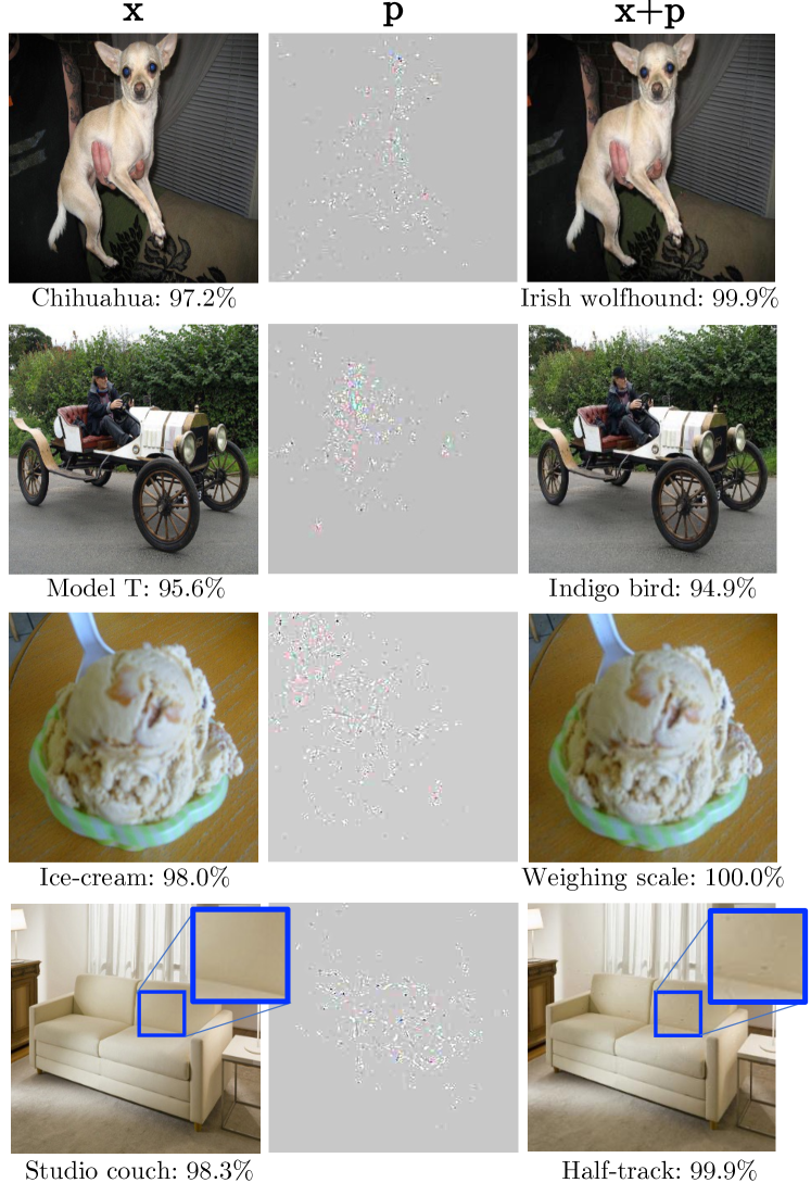
Figure 2: Qualitative results of targeted SAIF attack on Inception-v3 trained on ImageNet, using $\epsilon=100$ (39% of the dynamic range of image) and $k=400$ (0.15% of pixels). The source and target class, along with the corresponding probability, are stated below each $\mathbf{x}$ and $\mathbf{x+p}$ respectively.

Attack Saliency.

We use the following metric to capture the correspondence between the vulnerable and salient pixels in the input images. The score represents the overlap of the ground-truth (GT) bounding box of the subject of the input image with the (sparse) adversarial perturbation.

• Localization (Loc.) [6] Effectively the same as IoU for object detection. Given image pixels X, GT salient pixels S and SAIF sparse mask A, the localization score is:

  $$\text{Loc.}=\frac{\|A\cap S\|_{0}}{\|S\|_{0}+\|A\cap(X\setminus S)\|_{0}}$$ (7)

  In the event of perfect correspondence between the GT salient regions and adversarial perturbation, Loc.$\rightarrow$1. Whereas, Loc.$\rightarrow$0 when there is poor overlap between the two.

6 Results

Quantitative Results.

$\|\mathbf{p}\|_{\infty}\leq\epsilon$	Attacks	Inception-v3					ResNet50
		Sparsity ‘$k$’					Sparsity ‘$k$’
		10	20	50	100	200	10	20	50	100	200
$\epsilon$ = 255	SparseFool	1.59	4.39	15.37	32.14	32.14	1.79	3.19	8.78	17.76	33.33
	GreedyFool	3.99	7.58	16.57	35.33	62.87	4.19	7.78	21.76	42.12	72.26
	TSAA	0.00	0.00	0.00	0.00	2.02	0.00	0.00	0.00	1.95	16.06
	PGD $\ell_{0}+\ell_{\infty}$*	0.81	0.81	3.63	5.65	7.80	11.20	11.20	11.67	12.25	12.25
	SA-MOO*	9.52	10.04	14.28	38.09	39.47	27.98	44.32	45.12	54.83	60.91
	SAIF (Ours)	19.88	60.16	90.05	100.0	100.0	38.25	61.72	100.0	100.0	100.0
		10	20	50	100	200	10	20	50	100	200
$\epsilon$ = 100	SparseFool	0.79	3.39	9.98	27.54	48.90	1.39	2.59	7.58	19.56	35.72
	GreedyFool	2.39	3.79	10.18	23.15	45.11	2.20	5.99	15.77	34.73	61.68
	PGD $\ell_{0}+\ell_{\infty}$*	0.00	1.24	3.29	5.22	6.86	11.67	12.25	12.25	12.25	14.49
	SA-MOO*	4.67	9.52	9.98	14.28	23.81	29.86	34.10	35.56	39.83	50.24
	SAIF (Ours)	0.00	28.91	60.26	90.03	100.0	20.42	41.26	79.32	100.0	100.0
		200	500	1000	2000	3000	200	500	1000	2000	3000
$\epsilon$ = 10	SparseFool	4.19	14.17	38.92	67.86	82.24	11.98	39.92	69.46	90.02	95.61
	GreedyFool	8.78	22.55	40.52	65.07	77.25	18.77	47.70	74.65	93.41	97.21
	TSAA	0.00	0.00	0.00	0.00	0.00	0.00	0.00	0.00	0.59	6.89
	PGD $\ell_{0}+\ell_{\infty}$*	4.83	7.69	11.21	22.03	30.47	11.28	11.28	11.64	12.80	14.83
	SA-MOO*	4.76	4.98	5.02	9.52	10.98	15.56	17.82	18.01	18.94	20.97
	SAIF (Ours)	10.21	52.40	89.02	90.00	100.0	50.04	73.09	95.00	100.0	100.0

Table 2: Quantitative evaluation of untargeted attack on Inception-v3 and ResNet50 trained on ImageNet dataset. We report the ASR for varying constraints on sparsity ‘$k$’ and $\ell_{\infty}$-norm of the magnitude of perturbation ‘$\epsilon$’. Black-box attacks are marked with *.

We evaluate the ASR of all attack methods on a range of constraints on perturbation magnitude $\epsilon$ and sparsity $k$. The results for targeted attacks on ImageNet are reported in Table 1. The target class is randomly chosen for each sample. Note that TSAA [19] does not evaluate attacks for $\epsilon=100$. Moreover, for both targeted and untargeted attacks, SAPF [12] fails for all the evaluated thresholds.

Table 1 demonstrates that SAIF consistently outperforms both targeted attack baselines by a large margin for all $\epsilon$ and $k$ thresholds. For smaller $\epsilon$, GreedyFool fails to attack samples unless the sparsity threshold is significantly relaxed. A similar pattern is observed for the sparsity budget - competing attacks completely fail for tighter bounds on perturbation magnitude (see $\epsilon=10/100/255$ at $k=2000$). Moreover, at lower $k$, ResNet50 is easier to fool than Inception-v3.

We also compare the ASR for untargeted attacks against the baselines in Table 2. Here as well SAIF significantly outperforms other attacks, particularly on tighter perturbation bounds. By jointly optimizing over the two constraints, we are able to fool DNNs with extremely small distortions. For instance, at $\epsilon=10$, SAIF modifies only 0.37% pixels per image to successfully perturb 89.02% of input samples. This is more than twice the ASR of state-of-the-art sparse attack methods. Similarly, at $\epsilon=255$, only 0.03% pixels are attacked to achieve a perfect ASR. On CIFAR-10, SAIF achieves $\sim$3$\times$ higher ASR on lower sparsity thresholds. The results are reported in the Appendix.

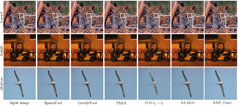
Figure 3: Visual results of untargeted attack on three images for $\epsilon=255$, $k=600$. Our method produces the most imperceptible adversarial examples despite the relaxed constraint on magnitude.

Note that sparse attacks like ours address a more challenging problem than $\ell_{\infty}$-norm threat models since both the perturbation magnitude and sparsity are to be constrained. For $\ell_{\infty}$ constraints $\epsilon=$10, 100, and 255, AutoAttack [10] achieves $100\%$ ASR with a perturbation sparsity of $\sim$98% for each $\epsilon$. For the same $\epsilon$, SAIF achieves $100\%$ ASR with 1.12%, 0.07%, and 0.037% sparsity, respectively. Moreover, sparse attacks are more visually interpretable than $\ell_{\infty}$ attacks.

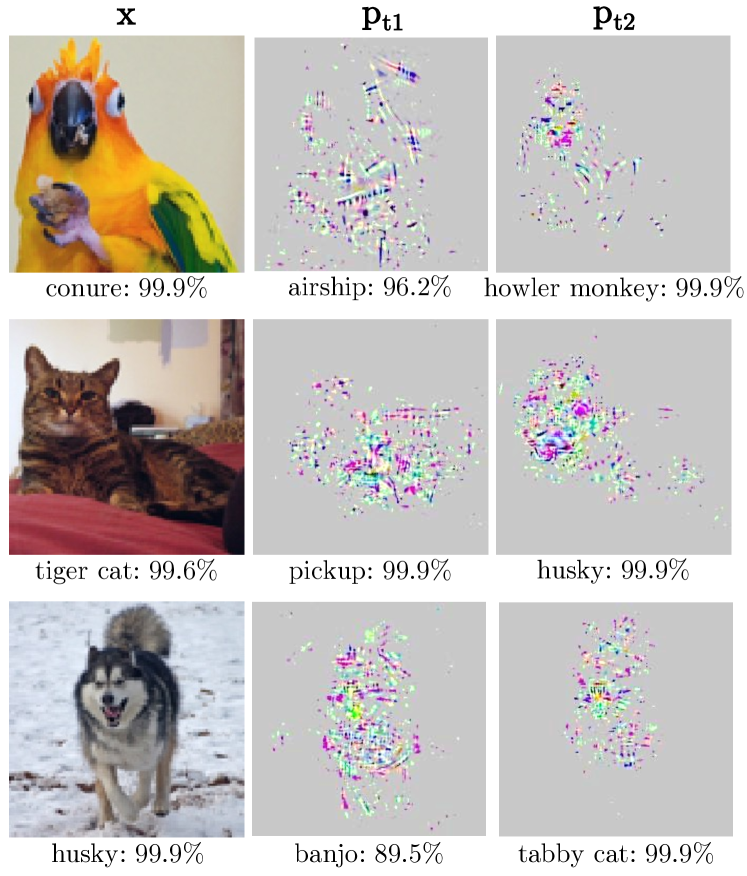
Figure 4: Impact of choice of target class on adversarial perturbations. We run targeted attacks for two target classes ($\mathbf{t_{1}}$ and $\mathbf{t_{2}}$) for each input. The perturbations have been enhanced for visualization.

Qualitative Results.

We include some examples of targeted adversarial examples using SAIF in Figure 2. Note that the perturbations $\mathbf{p}$ have been enhanced in all figures for visibility. Visually, the perturbations generated by SAIF are only slightly noticeable in regions with a uniform color palette/low textural detail, such as on the beige couch (see the zoomed-in segments of Figure 2). The other images are bereft of such regions and thus have negligible visible change. Moreover, we observe that the attack predominantly perturbs semantically meaningful pixels in the images.

For untargeted attacks, we present examples from all competing attack methods in Figure 3. We ease the magnitude constraint to allow all baselines to achieve some successful attacks at the same level of sparsity. It can be observed that all competing methods produce highly conspicuous perturbations around the face of the leopard, and on the outlines of the forklift and the albatross. PGD $\ell_{\infty}+\ell_{0}$, in particular, adds the most noticeable distortions to images. In contrast, SAIF attack produces adversarial examples that appear virtually identical to the clean input images.

Perturbations and Interpretability

Attack	Loc. $\uparrow$
SparseFool	0.006
GreedyFool	0.001
TSAA	0.006
SAIF (untargeted)	0.126
SAIF (targeted)	0.118

Table 3: Quantitative evaluation of interpretability in terms of overlap with GT bounding boxes of ImageNet validation images. We use $\epsilon=255,k=200$ for all attacks in an untargeted setting unless indicated otherwise.

The sparse nature of perturbations allows us to study the interpretability of each attack (i.e. their correspondence with discriminative image regions). A similar evaluation is carried out in [39], but they treat the saliency maps obtained from CAM [40] as the ground truth. The saliency maps from CAM (and other existing methods) incur several failure cases. Therefore, we use the ImageNet bounding box annotations as a reliable baseline to analyze attack understandability.

We use ResNet50 as the target model and set $\epsilon=255$ and $k=2000$ for all attacks. The results are reported in Table 3. SAIF achieves the highest Loc. score among competing methods in both the targeted and untargeted attack setting. Note that SAIF performs better on this metric in the untargeted attack setting versus the targeted attack. This is intuitive since the untargeted objective only diminishes features of the true class. Whereas, targeted attacks introduce features to convince a DNN to predict the target class.

Moreover, from visual inspection (see Figure 4) it is observed that the nature of the target class also determines the sparse distortion pattern. In particular, attacking input images of an animate class towards another animate class ($t_{2}$) results in perturbations focused predominantly on the facial region in the image. The reverse is observed when attacking animate towards inanimate object classes ($t_{1}$), which typically modify the body of the subject in the image.

6.1 Speed Comparison

Attack	Time (sec)
SparseFool	20
GreedyFool	1.7
TSAA	1.8
SAPF	1142
Homotopy-Attack	1500
PGD $\ell_{0}+\ell_{\infty}$	1.46
SA-MOO	56.07
SAIF (ours)	15

Table 4: Average running times on ImageNet

Table 4 reports the running times of all baselines. PGD $\ell_{0}+\ell_{\infty}$ [9] runs the fastest but produces the most noticeable perturbations. Note that, although the inference time for GreedyFool [11] and TSAA [19] is $\leq 2$ seconds, these generator-based attacks require pre-training a generator for each target model (as well as each $\epsilon$ and target class for TSAA [19]). This incurs a significant computational overhead ($>$7 days on a single GPU), which offsets their faster convergence times. SAIF attack relies solely on pre-trained classifiers, and is significantly faster than the existing state-of-the-art Homotopy-Attack [41]. More efficient implementations of the FW LMO can further shorten running times, which we leave for future work.

7 Ablation Studies

We perform two sets of ablative experiments to highlight the significance of our design choices.

Attack Sparsity.

To illustrate the importance of limiting the sparsity of attack using $\mathbf{s}$, we reformulate the problem to one constrained only over the perturbation magnitude. That is, we use the following objective for the untargeted attack:

$$D(\mathbf{p})_{adv}=\Phi(\mathbf{x}+\mathbf{p},c)$$ (8)

$$\max_{\mathbf{p}}D(\mathbf{p})_{adv},\ \text{ s.t. }\quad\|\mathbf{p}\|_{\infty}\leq\epsilon$$ (9)

Similarly, we reframe the targeted attack by optimizing for the objective $D(\mathbf{p})_{adv}$ where,

$$D(\mathbf{p})_{t,adv}=\Phi(\mathbf{x}+\mathbf{p},t)$$ (10)

$$\min_{\mathbf{p}}D(\mathbf{p})_{t,adv},\ \text{ s.t. }\quad\|\mathbf{p}\|_{\infty}\leq\epsilon$$ (11)

This is similar to [7]’s attack method that uses Frank-Wolfe for optimization.

Following Table 1-2, we test the attack for various $\epsilon$ and report the results in Table 5. It is observed that in the absence of a sparsity constraint, the attack distorts all image pixels regardless of the constraint on magnitude. Moreover, such spatially ‘contiguous’ perturbations are visible even at magnitudes as low as $\epsilon=10$ (see Figure 5). By constraining the sparsity for SAIF attack, we ensure the adversarial perturbations stay imperceptible even at $\epsilon=255$, at which the non-sparse attack completely obfuscates the image.

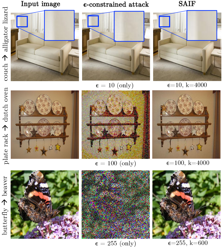
Figure 5: Exploring the significance of sparsity of the adversarial attack. When the sparsity is not constrained (middle column), perturbations of very small magnitude ($\epsilon=10$) are noticeable and completely distort the image for larger $\epsilon$. On the contrary, SAIF (third column) stays imperceptible at higher magnitudes as well.

Attack Type	Dataset	ASR $\uparrow$	$||\mathbf{p}||_{0}/m$ $\downarrow$
untargeted	$\epsilon=255$	100.0	1.0
	$\epsilon=100$	100.0	1.0
	$\epsilon=10$	100.0	1.0
targeted	$\epsilon=255$	100.0	1.0
	$\epsilon=100$	100.0	1.0
	$\epsilon=10$	100.0	1.0

Table 5: Quantitative evaluation of optimizing SAIF without a sparsity constraint for Inception-v3 on ImageNet. For each perturbation magnitude, the attack distorts all the pixels in the image leading to high perceptibility.

Constraints	ASR
$\epsilon=255,k=600$	97.78%
$\epsilon=100,k=600$	98.30%
$\epsilon=10,k=3000$	88.97%

Table 6: ASR for targeted attacks on Inception-v3 when cross-entropy is replaced with $\ell_{2}$-attack loss [4].

Loss formulation.

We also experiment with different losses, mainly the $\ell_{2}$-attack proposed by [4], but observe a decline in attack success (see Table 6. We choose $\epsilon$ and $k$ for which SAIF achieves 100% ASR in Table 1.). A possible explanation for this behavior is that the loss formulation tries to increase the target class probability too aggressively, which makes the simultaneous optimization of $\mathbf{s}$ and $\mathbf{p}$ difficult. We observe that this yields solutions closer to the constraint boundaries, increasing the attack visibility.

8 Conclusion

In this work, we propose a novel adversarial attack, ‘SAIF’, by jointly minimizing the magnitude and sparsity of perturbations. By constraining the attack sparsity, we not only conceal the attacks but also identify the most vulnerable pixels in natural images. We use the Frank-Wolfe algorithm to optimize our objective and achieve effective convergence, with reasonable efficiency, for large natural images. We perform comprehensive experiments against state-of-the-art attack methods and demonstrate the remarkably superior performance of SAIF under tight magnitude and sparsity budgets. Our method also outperforms existing methods on a quantitative metric for interpretability and provides transparency to visualize vulnerabilities of DNNs.

Discussion

Social Impact

Adversarial attacks expose the fragility of DNNs. Our work aims at demonstrating that a highly imperceptible adversarial attack can be generated for natural images. This provides a new benchmark for the research community to test the robustness of the learning algorithms. A straightforward defense strategy can be using the adversarial examples generated by SAIF for adversarial training. We leave more advanced solutions for further exploration.

Results on additional dataset

We also test our approach on a smaller dataset for a comprehensive evaluation of our attacks.

Dataset and model

We test SAIF and the existing sparse attack algorithms on the CIFAR-10 dataset [22]. The dataset comprises of $[32\times 32]$ RGB images belonging to 10 classes. We evaluate all algorithms on 10,000 samples from the test set.

We attack VGG-16 [14] trained on CIFAR-10, having an accuracy of 92.32% on clean images.

Quantitative Results

We run all attacks for a range of $\epsilon$ and $k$, and report the results in Tables 7,8.

The ASR for the untargeted attack is reported in Table 7. SAIF consistently outperforms SparseFool [27] and GreedyFool [11] on all sparsity and magnitude constraints. Similar results for targeted attacks are reported in Table 8. The target classes are randomly chosen in all experiments.

Qualitative Results

We provide several examples of adversarial examples produced by SAIF and competing algorithms. Figure 6 shows samples obtained by untargeted attacks on VGG-16 trained on CIFAR-10. It is observed that SAIF consistently produces the most imperceptible perturbations.

$\|\mathbf{p}\|_{\infty}\leq\epsilon$	Attacks	VGG-16
		Sparsity ‘$k$’
		1	2	5	10	20
$\epsilon$ = 255	SparseFool [27]	10.78	18.56	38.32	63.67	85.23
	GreedyFool [11]	0.00	0.00	24.75	69.26	85.83
	SAIF (Ours)	91.20	92.87	94.46	96.35	100.0
		5	10	15	20	30
$\epsilon$ = 100	SparseFool [27]	30.54	51.50	65.47	74.45	86.43
	GreedyFool [11]	25.95	55.09	67.26	73.65	86.43
	SAIF (Ours)	91.89	92.84	93.57	96.74	97.80
		30	40	50	60	100
$\epsilon$ = 10	SparseFool [27]	19.36	24.75	27.94	31.94	44.51
	GreedyFool [11]	33.93	39.92	45.91	51.10	66.27
	SAIF (Ours)	90.32	91.57	92.14	92.65	94.14

Table 7: Quantitative evaluation of untargeted attack on CIFAR-10. We report the ASR for varying constraints on sparsity ‘$k$’ and $\ell_{\infty}$-norm of the magnitude of perturbation ‘$\epsilon$’.

$\|\mathbf{p}\|_{\infty}\leq\epsilon$	Attacks	VGG-16
		Sparsity ‘$k$’
		1	2	5	10	20
$\epsilon$ = 255	GreedyFool [11]	0.00	0.00	2.79	13.17	29.94
	SAIF (Ours)	12.36	12.83	27.02	44.05	61.10
		5	10	15	20	30
$\epsilon$ = 100	GreedyFool [11]	2.20	9.58	14.97	16.97	30.74
	SAIF (Ours)	13.37	21.03	26.27	36.18	51.43
		30	40	50	60	100
$\epsilon$ = 10	GreedyFool [11]	3.99	5.19	6.99	8.98	16.17
	SAIF (Ours)	5.46	13.35	18.13	22.25	29.26

Table 8: Quantitative evaluation of targeted attack on CIFAR-10. We report the ASR for varying constraints on sparsity ‘$k$’ and $\ell_{\infty}$-norm of the magnitude of perturbation ‘$\epsilon$’.

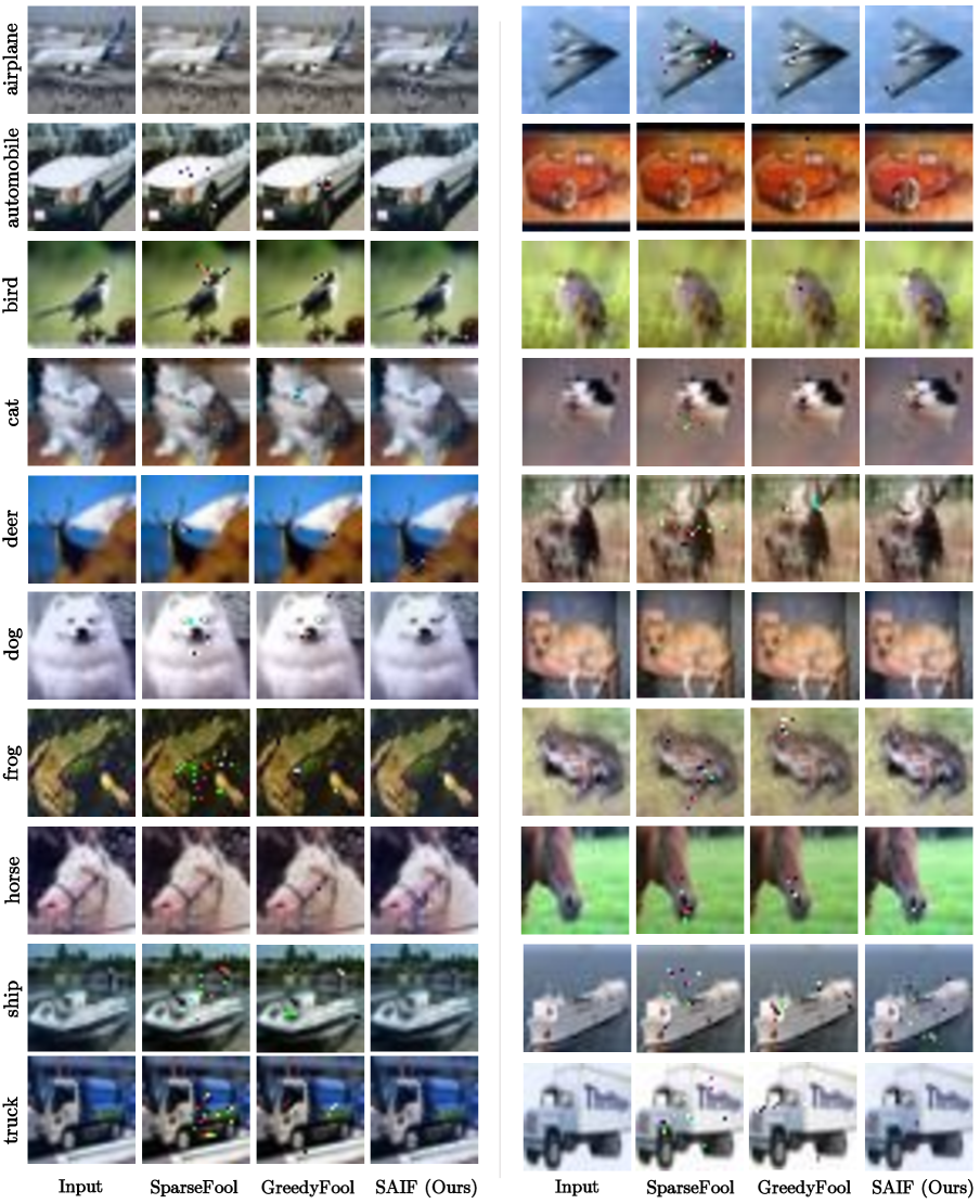
Figure 6: Untargeted adversarial examples obtained from SAIF and competing attack algorithms on CIFAR-10. The attacked classifier is VGG-16

References

- [1] Philipp Benz, Chaoning Zhang, Tooba Imtiaz, and In So Kweon. Double targeted universal adversarial perturbations. In Proceedings of the Asian Conference on Computer Vision, 2020.
- [2] Mathieu Besançon, Alejandro Carderera, and Sebastian Pokutta. FrankWolfe.jl: a high-performance and flexible toolbox for Frank-Wolfe algorithms and Conditional Gradients, 2021. https://arxiv.org/abs/2104.06675.
- [3] Alejandro Carderera, Mathieu Besançon, and Sebastian Pokutta. Simple steps are all you need: Frank-wolfe and generalized self-concordant functions. Advances in Neural Information Processing Systems, 34:5390–5401, 2021.
- [4] Nicholas Carlini and David Wagner. Towards evaluating the robustness of neural networks. In 2017 ieee symposium on security and privacy (sp), pages 39–57. IEEE, 2017.
- [5] Varun Chandola, Arindam Banerjee, and Vipin Kumar. Anomaly detection: A survey. ACM computing surveys (CSUR), 41(3):1–58, 2009.
- [6] Aditya Chattopadhay, Anirban Sarkar, Prantik Howlader, and Vineeth N Balasubramanian. Grad-cam++: Generalized gradient-based visual explanations for deep convolutional networks. In 2018 IEEE winter conference on applications of computer vision (WACV), pages 839–847, 2018.
- [7] Jinghui Chen, Dongruo Zhou, Jinfeng Yi, and Quanquan Gu. A frank-wolfe framework for efficient and effective adversarial attacks. Proceedings of the AAAI Conference on Artificial Intelligence, 34(04):3486–3494, Apr. 2020.
- [8] François Chollet et al. Keras. https://keras.io/api/applications/, 2015.
- [9] Francesco Croce and Matthias Hein. Sparse and imperceivable adversarial attacks. In Proceedings of the IEEE/CVF International Conference on Computer Vision, pages 4724–4732, 2019.
- [10] Francesco Croce and Matthias Hein. Reliable evaluation of adversarial robustness with an ensemble of diverse parameter-free attacks. In International conference on machine learning, pages 2206–2216. PMLR, 2020.
- [11] Xiaoyi Dong, Dongdong Chen, Jianmin Bao, Chuan Qin, Lu Yuan, Weiming Zhang, Nenghai Yu, and Dong Chen. Greedyfool: Distortion-aware sparse adversarial attack. Advances in Neural Information Processing Systems, 33:11226–11236, 2020.
- [12] Yanbo Fan, Baoyuan Wu, Tuanhui Li, Yong Zhang, Mingyang Li, Zhifeng Li, and Yujiu Yang. Sparse adversarial attack via perturbation factorization. In Computer Vision–ECCV 2020: 16th European Conference, Glasgow, UK, August 23–28, 2020, Proceedings, Part XXII 16, pages 35–50. Springer, 2020.
- [13] Marguerite Frank, Philip Wolfe, et al. An algorithm for quadratic programming. Naval research logistics quarterly, 3(1-2):95–110, 1956.
- [14] Yonatan Geifman. Vgg16 models for cifar-10 and cifar-100 using keras, 2019. https://github.com/geifmany/cifar-vgg.
- [15] Gauthier Gidel, Fabian Pedregosa, and Simon Lacoste-Julien. Frank-wolfe splitting via augmented lagrangian method. In Proceedings of the Twenty-First International Conference on Artificial Intelligence and Statistics, volume 84 of Proceedings of Machine Learning Research, pages 1456–1465. PMLR, 2018.
- [16] Ross Girshick. Fast r-cnn. In Proceedings of the IEEE international conference on computer vision, pages 1440–1448, 2015.
- [17] Ian Goodfellow, Jonathon Shlens, and Christian Szegedy. Explaining and harnessing adversarial examples. In International Conference on Learning Representations, 2015.
- [18] Kaiming He, Xiangyu Zhang, Shaoqing Ren, and Jian Sun. Deep residual learning for image recognition. In Proceedings of the IEEE conference on computer vision and pattern recognition, pages 770–778, 2016.
- [19] Ziwen He, Wei Wang, Jing Dong, and Tieniu Tan. Transferable sparse adversarial attack. In Proceedings of the IEEE/CVF Conference on Computer Vision and Pattern Recognition, pages 14963–14972, 2022.
- [20] Alexey Ignatiev, Nina Narodytska, and Joao Marques-Silva. On relating explanations and adversarial examples. Advances in neural information processing systems, 2019.
- [21] Martin Jaggi. Revisiting frank-wolfe: Projection-free sparse convex optimization. In International Conference on Machine Learning, pages 427–435. PMLR, 2013.
- [22] Alex Krizhevsky et al. Learning multiple layers of features from tiny images. 2009.
- [23] Alex Krizhevsky, Ilya Sutskever, and Geoffrey E Hinton. Imagenet classification with deep convolutional neural networks. In Advances in Neural Information Processing Systems, volume 25, pages 1097–1105. Curran Associates, Inc., 2012.
- [24] Simon Lacoste-Julien. Convergence rate of frank-wolfe for non-convex objectives. arXiv preprint arXiv:1607.00345, 2016.
- [25] Jan Macdonald, Mathieu E. Besançon, and Sebastian Pokutta. Interpretable neural networks with frank-wolfe: Sparse relevance maps and relevance orderings. In Proceedings of the 39th International Conference on Machine Learning, volume 162 of Proceedings of Machine Learning Research, pages 14699–14716. PMLR, 2022.
- [26] Aleksander Madry, Aleksandar Makelov, Ludwig Schmidt, Dimitris Tsipras, and Adrian Vladu. Towards deep learning models resistant to adversarial attacks. In International Conference on Learning Representations, 2018.
- [27] Apostolos Modas, Seyed-Mohsen Moosavi-Dezfooli, and Pascal Frossard. Sparsefool: a few pixels make a big difference. In Proceedings of the IEEE/CVF conference on computer vision and pattern recognition, pages 9087–9096, 2019.
- [28] Seyed-Mohsen Moosavi-Dezfooli, Alhussein Fawzi, and Pascal Frossard. Deepfool: a simple and accurate method to fool deep neural networks. In Proceedings of the IEEE conference on computer vision and pattern recognition, pages 2574–2582, 2016.
- [29] Nina Narodytska and Shiva Prasad Kasiviswanathan. Simple black-box adversarial attacks on deep neural networks. In CVPR Workshops, volume 2, page 2, 2017.
- [30] Nicolas Papernot, Patrick McDaniel, Somesh Jha, Matt Fredrikson, Z Berkay Celik, and Ananthram Swami. The limitations of deep learning in adversarial settings. In 2016 IEEE European symposium on security and privacy (EuroS&P), pages 372–387. IEEE, 2016.
- [31] Joseph Redmon, Santosh Divvala, Ross Girshick, and Ali Farhadi. You only look once: Unified, real-time object detection. In Proceedings of the IEEE conference on computer vision and pattern recognition, pages 779–788, 2016.
- [32] Jay Roberts and Theodoros Tsiligkaridis. Controllably Sparse Perturbations of Robust Classifiers for Explaining Predictions and Probing Learned Concepts. In Machine Learning Methods in Visualisation for Big Data. The Eurographics Association, 2021.
- [33] Jiawei Su, Danilo Vasconcellos Vargas, and Kouichi Sakurai. One pixel attack for fooling deep neural networks. IEEE Transactions on Evolutionary Computation, 23(5), 2019.
- [34] Christian Szegedy, Wojciech Zaremba, Ilya Sutskever, Joan Bruna, Dumitru Erhan, Ian Goodfellow, and Rob Fergus. Intriguing properties of neural networks. In International Conference on Learning Representations, 2014.
- [35] Theodoros Tsiligkaridis and Jay Roberts. Understanding and increasing efficiency of frank-wolfe adversarial training. In Proceedings of the IEEE/CVF Conference on Computer Vision and Pattern Recognition, pages 50–59, 2022.
- [36] Yisen Wang, Xingjun Ma, James Bailey, Jinfeng Yi, Bowen Zhou, and Quanquan Gu. On the convergence and robustness of adversarial training. In Proceedings of the 36th International Conference on Machine Learning, Proceedings of Machine Learning Research. PMLR, 2019.
- [37] Zifan Wang, Matt Fredrikson, and Anupam Datta. Robust models are more interpretable because attributions look normal. In Proceedings of the 39th International Conference on Machine Learning, volume 162 of Proceedings of Machine Learning Research, pages 22625–22651. PMLR, 2022.
- [38] Phoenix Neale Williams and Ke Li. Black-box sparse adversarial attack via multi-objective optimisation. In Proceedings of the IEEE/CVF Conference on Computer Vision and Pattern Recognition, pages 12291–12301, 2023.
- [39] Kaidi Xu, Sijia Liu, Pu Zhao, Pin-Yu Chen, Huan Zhang, Quanfu Fan, Deniz Erdogmus, Yanzhi Wang, and Xue Lin. Structured adversarial attack: Towards general implementation and better interpretability. In International Conference on Learning Representations, 2019.
- [40] Bolei Zhou, Aditya Khosla, Agata Lapedriza, Aude Oliva, and Antonio Torralba. Learning deep features for discriminative localization. In Proceedings of the IEEE conference on computer vision and pattern recognition, pages 2921–2929, 2016.
- [41] Mingkang Zhu, Tianlong Chen, and Zhangyang Wang. Sparse and imperceptible adversarial attack via a homotopy algorithm. In ICML. PMLR, 2021.