Second-order force scheme for lattice Boltzmann method

Abstract

We present an a priori derivation of the force scheme for lattice Boltzmann method based on kinetic theoretical formulation. We show that the discrete lattice effect, previously eliminated a posteriori in BGK collision model, is due to first-order space-time discretization and can be eliminated generically for a wide range of collision models with second-order space-time discretization. Particularly, the force scheme for the recently developed spectral multiple-relaxation-time (SMRT) collision model is obtained and numerically verified.

I Introduction

Since the early development of lattice Boltzmann method (LBM), implementation of the body force term has been generating continued interests [1]. This is especially true in recent years as more complex collision models are adopted in place of the Bhatnagar-Gross-Krook (BGK) [24] model, and LBM applied to multiphase flows where the interaction is modeled by a Vlasov body force [2, 3]. Both trends call for more accurate treatment of the body force term. Literally a dozen force schemes have been proposed and extensive numerical evaluations conducted [4, 5]. Nevertheless, conclusion has not been reached on how the force term should be implemented independent of the details of the collision model and underlying lattice.

One of the earliest force schemes is the intuitive velocity-shift method used in the modeling of inter-molecular interactions [2]. This method shifts the velocity in the equilibrium distribution by $\bm{g}\Delta t$, where $\bm{g}$ is the acceleration and $\Delta t$ the time step. A more refined scheme [6] eliminated the discrete lattice effect by introducing unknown coefficients in the force term and determining them by matching the recovered macroscopic equation with Navier-Stokes equations. Benchmarks in the context of non-ideal gas showed that with the velocity-shift scheme, the equilibrium densities has an un-physical dependence on the relaxation time whereas with the latter scheme this abnormality is completely eliminated [7]. Li et al. [8] analyzed the exact difference method (EDM) [9], and found that its great stability in Shan-Chen (SC) model  [2] attributes to the extra error introduced to the pressure tensor. Furthermore, Li et al. [8] proposed an improved force scheme to deal with the high-density ratio in the SC model. Several force schemes for the central-moment multiple-relaxation-time collision models with standard lattice have also been developed [10, 11, 12].

It is worth noting that in terms of the hydrodynamic moments, the leading effect of all the models are unanimously the same, namely, when considered as an addition to the normal collision term, the zeroth moment of the body force term vanishes to ensure mass conservation and the first moment equals to $\bm{g}\Delta t$. The subtle differences are only in the second and higher moments representing the additional momentum and energy fluxes caused by the body force. This effect manifests in cases such as multiphase flow modeling where the additional stress plays a significant role [7].

The complexity and controversy are partially due to the fact that the development of the force schemes mostly followed the same a posteriori approach of the LB development. The LB equation is constructed as a kinetic model fully discretized in both the velocity and configuration spaces with a discretized time. The errors caused by all discretizations are then optimized to achieve the correct macroscopic Navier-Stokes equation. Besides being disconnected from the Boltzmann equation which includes the effect of the body force, the multiple expansion approach quickly becomes unmanageable for more complex collision models.

In the kinetic theoretical formulation of LB [13, 14], the LB equation is obtained by first discretizing the continuum Boltzmann-BGK equation in the velocity space, resulting in a set of partial differential equations in the normal space and time for a set of discrete-velocity distribution function. Without any ambiguity, the body force is given by the finite Hermite expansion of the body force term [15, 14]. However, to further discretize the space and time with a finite difference scheme, multiple schemes exist.

In the present work we first show that the scheme of Guo et al [6] can be obtained a priori by further discretizing the discrete-velocity Boltzmann equation with the second-order finite difference in space and time. The same finite difference scheme can be applied to the recently suggested SMRT collision model [16, 17, 18].

The LBE is obtained by further discretizing Eq. (19) in space and time using first-order forward-Euler finite difference scheme. It was shown by multiple expansions that after absorbing the leading order error into the dissipation term, the scheme is effectively second-order with a viscosity proportional to $\tau+1/2$ instead of $\tau$ [19]. In presence of a body force, the discrete lattice effect can be eliminated [6] a posteriori. We show in this section that the same correction can be obtained a priori for the BGK model by integrating Eq. (19) using second-order quadrature rules [20]. In the next section, the same technique is used to obtain the force scheme for the Hermite-space MRT model.

With the BGK collision model, the description of the collision as a uniform relaxation process of the distribution function towards its equilibrium is in many cases simplistic. In a previous series of papers [21, 18, 22], the SMRT collision model was developed where the irreducible components of the Hermite coefficients are relaxed separately in the reference frame moving with the fluid. These components are the minimum tensor components that can be separately relaxed without violating rotation symmetry.

The rest of the paper is organized as the following. The theoretical derivation is presented in Section II with the discrete-velocity force scheme presented in Section II.1, the derivation of the force scheme for BGK model in Section II.2, and force scheme for the SMRT collision model in Section II.3. Some numerical verification is given in Section III and the conclusion and discussions are given in Sec. IV.

II Boltzmann-BGK equation

II.1 Background

In kinetic theory [23], the evolution of the single-particle distribution, $f(\bm{x},\bm{\xi},t)$, under an external or self-generated body force with acceleration $\bm{g}$ is described by the Boltzmann equation:

$$\frac{\partial f}{\partial t}+\bm{\xi}\cdot\nabla f+\bm{g}\cdot\nabla_{\bm{\xi}}f=\Omega(f),$$ (1)

where, $\bm{x}$ and $\bm{\xi}$ are coordinates in physical and velocity spaces respectively, $t$ the time, $\Omega(f)$ the collision term describing the effect of inter-particle collision. Due to its extreme complexity, the collision term is often simplified by models, of which the most widely used is the BGK model:

$$\Omega_{BGK}(f)=-\frac{1}{\tau}\left[f-f^{(eq)}\right],$$ (2)

where $\tau$ is a relaxation time and $f^{(eq)}$ the Maxwell-Boltzmann distribution. Choosing the characteristic speed $\sqrt{k_{B}T_{0}/m_{0}}$ with $k_{B}$ the Boltzmann constant and $T_{0}$ and $m_{0}$ the reference temperature and molecule mass, $f^{(eq)}$ has the dimensionless form

$$f^{(eq)}(\bm{x},\bm{\xi},t)=\frac{\rho}{(2\pi\theta)^{D/2}}\exp\left[-\frac{(\bm{\xi}-\bm{u})^{2}}{2\theta}\right],$$ (3)

where $\rho$ is the density, $\bm{u}$ the fluid velocity and $\theta\equiv T/T_{0}$ the temperature, all dimensionless.

The lattice Boltzmann equation was formulated as a special velocity-space discretization of the Boltzmann equation based on two observations [14]. First, in Chapman-Enskog calculation [25], the macroscopic hydrodynamics only depends on the leading moments of the distribution function rather than its entirety. The distribution function can therefore be approximated by its low-order Hermite expansion without altering the hydrodynamics [26, 27]. This truncation is equivalent to projecting Eq. (1) into a low-order Hilbert space spanned by the Hermite polynomials. Denoting the $N$-th order Hermite series by:

$$f_{N}(\bm{x},\bm{\xi},t)=\omega(\bm{\xi})\sum_{n=0}^{N}\frac{1}{n!}\bm{a}^{(n)}:{\cal H}^{(n)}(\bm{\xi}),$$ (4)

where ${\cal H}^{(n)}(\bm{\xi})$ is the $n$-th Hermite polynomial, and

$$\omega(\bm{\xi})\equiv(2\pi)^{-D/2}\exp\left(-\xi^{2}/2\right),$$ (5)

is the weight function with respect to which the Hermite polynomials are orthogonal. The expansion coefficients:

$$\bm{a}^{(n)}(\bm{x},t)=\int f_{N}(\bm{x},\bm{\xi},t){\cal H}^{(n)}(\bm{\xi})d\bm{\xi},$$ (6)

are velocity moments of the distribution function with the leading few being the familiar hydrodynamic variables, $\rho$, $\bm{u}$ and $\theta$.

Second, any finite Hermite series is completely determined by its values on a finite set of $\bm{\xi}_{i}$. Let $\{(w_{i},\bm{\xi}_{i}),i=1,\cdots,d\}$ be the weights and abscissas of a $Q$-th degree Hermite quadrature such that for any $Q$-th degree polynomial, $p(\bm{\xi})$, we have:

$$\int\omega(\bm{\xi})p(\bm{\xi})d\bm{\xi}=\sum_{i=0}^{d}w_{i}p(\bm{\xi}_{i}).$$ (7)

The $M$-th moment of $f_{N}$ is then

$$\int f_{N}(\bm{\xi})\bm{\xi}^{M}d\bm{\xi} = \int\omega(\bm{\xi})\left[\frac{f_{N}(\bm{\xi})\bm{\xi}^{M}}{\omega(\bm{\xi})}\right]d\bm{\xi}$$ (8)

$$= \sum_{i=0}^{d}\frac{w_{i}f_{N}(\bm{\xi}_{i})\bm{\xi}_{i}^{M}}{\omega(\bm{\xi}_{i})},$$

provided that $Q\geq M+N$, as the integrand in the brackets is a polynomial of degree $M+N$. Hence, all expansion coefficients are completely determined by $f_{N}(\bm{\xi}_{i})$ as long as $\{\bm{\xi}_{i}\}$ forms the abscissas of a quadrature rule of a degree $Q\geq 2N$. If we further define the convenience variable:

$$f_{i}\equiv\frac{w_{i}f_{N}(\bm{x},\bm{\xi}_{i},t)}{\omega(\bm{\xi}_{i})},$$ (9)

the integral velocity moments has the discrete form:

$$\int f_{N}(\bm{\xi})\bm{\xi}^{M}d\bm{\xi}=\sum_{i=0}^{d}f_{i}\bm{\xi}_{i}^{M},$$ (10)

provided that the quadrature conditions are met. Noting by Eq. (6) that the expansion coefficients are also velocity moments, $\bm{a}^{(n)}$ and $f_{i}$ can be transformed through the following general discrete Fourier transform:

$$\bm{a}^{(n)} = \sum_{i=0}^{d}f_{i}{\cal H}^{(n)}(\bm{\xi}_{i}),$$ (11a)

$$f_{i} = w_{i}\sum_{n=0}^{N}\frac{1}{n!}\bm{a}^{(n)}:{\cal H}^{(n)}(\bm{\xi}_{i}).$$ (11b)

The dynamic equations of $f_{i}$ are taken as the direct evaluation of the projected Eq. (1) at $\bm{\xi}_{i}$. This amounts to expanding all terms in terms of Hermite polynomials and truncating to a finite order. The expansion of $\nabla_{\bm{\xi}}f_{N}$ can be obtained by taking the velocity-space derivative of Eq. (4) and using the following Rodrigues formula:

$${\cal H}^{(n)}(\bm{\xi})=\frac{(-1)^{n}}{\omega(\bm{\xi})}\nabla^{n}_{\bm{\xi}}\omega(\bm{\xi}),$$ (12)

to write:

$$\nabla_{\bm{\xi}}f_{N}=\sum_{n=0}^{N}\frac{1}{n!}\bm{a}^{(n)}:\nabla_{\bm{\xi}}\left[\omega(\bm{\xi}){\cal H}^{(n)}(\bm{\xi})\right]$$ (13)

$$= -\omega(\bm{\xi})\sum_{n=0}^{N}\frac{1}{n!}\bm{a}^{(n)}:{\cal H}^{(n+1)}(\bm{\xi})$$

$$= -\omega(\bm{\xi})\sum_{n=1}^{N+1}\frac{1}{n!}\left[n\bm{a}^{(n-1)}\right]:{\cal H}^{(n)}(\bm{\xi}).$$

The body-force term, denoted by $F(\bm{\xi})\equiv-\bm{g}\cdot\nabla_{\bm{\xi}}f_{N}$, has thus the following expansion:

$$F(\bm{\xi})=\omega(\bm{\xi})\sum_{n=1}^{N}\frac{1}{n!}\left[n\bm{g}\bm{a}^{(n-1)}\right]:{\cal H}^{(n)}(\bm{\xi}),$$ (14)

Denoting the Hermite coefficients of $F(\bm{\xi})$ by $\bm{a}^{(n)}_{F}$, we have

$$\bm{a}^{(0)}_{F}=0,\quad\mbox{and}\quad\bm{a}^{(n)}_{F}=n\bm{g}\bm{a}^{(n-1)},\quad n\geq 1.$$ (15)

where $\bm{g}\bm{a}^{(n-1)}$ is to be understood as the symmetric product between $\bm{g}$ and $\bm{a}^{(n-1)}$, e.g., in component form, $\bm{g}\bm{a}^{(2)}=(g_{\alpha}a_{\beta\gamma}+g_{\beta}a_{\gamma\alpha}+g_{\gamma}a_{\alpha\beta})/3$.

The explicit expressions for the first several orders of $\bm{a}^{(n)}_{0}$ can be found in the literature  [14]. Thus we have the expanded force term up to the fourth-order:

$$F\thickapprox\omega(\bm{\xi})\rho\{\underbrace{\bm{g}\cdot\bm{\xi}}_{1st}+\underbrace{(\bm{g}\cdot\bm{\xi})(\bm{\xi}\cdot\bm{u})-\bm{g}\cdot\bm{u}}_{2nd}$$

$$+\underbrace{\frac{1}{6\rho}3\bm{g}\left[\rho(\bm{u}^{2}+(\theta-1)\bm{\delta})+\bm{a}^{(2)}_{1}\right]:{\cal H}^{(3)}(\bm{\xi})}_{3rd}$$

$$+\underbrace{\frac{1}{24\rho}4\bm{g}(\bm{a}^{(3)}_{0}+\bm{a}^{(3)}_{1}):{\cal H}^{(4)}(\bm{\xi})}_{4th}\}\qquad$$ (16)

If the expansion of the force term is truncated to second order, the familiar force term can be obtained:

$$F(\bm{\xi})=\rho\omega(\bm{\xi})\left[\bm{g}\cdot(\bm{\xi}-\bm{u})+(\bm{g}\cdot\bm{\xi})(\bm{u}\cdot\bm{\xi})\right].$$ (17)

Similar to Eq. (9), defining:

$$F_{i}\equiv\frac{w_{i}F(\bm{\xi}_{i})}{\omega(\bm{\xi}_{i})},$$ (18)

the discrete-velocity Boltzmann equation with body force is:

$$\frac{\partial f_{i}}{\partial t}+\bm{\xi}_{i}\cdot\nabla f_{i}=\Omega_{i}+F_{i},\quad i=1,\cdots,d.$$ (19)

The above equation was previously given by Martys et al [15] and its relations to the previous models were also analyzed. Naturally the body force term is independent of the collision term, and other than the truncation order, there is no ambiguity.

II.2 force in BGK collision model

The LBE is obtained by further discretizing Eq. (19) in space and time using first-order forward-Euler finite difference scheme. It was shown by multiple expansions that after absorbing the leading order error into the dissipation term, the scheme is effectively second-order with a viscosity proportional to $\tau+1/2$ instead of $\tau$ [19]. In presence of a body force, the discrete lattice effect can be eliminated [6] a posteriori. We show in this section that the same correction can be obtained a priori for the BGK model by integrating Eq. (19) using second-order quadrature rules [20, 28, 29]. In the next section, the same technique is used to obtain the force scheme for the Hermite-space MRT model.

The discrete-velocity BGK model can be written as:

$$\Omega_{i}=-\frac{1}{\tau}\left[f_{i}-f_{i}^{(eq)}\right],$$ (20)

where:

$$f^{(eq)}_{i}=\rho w_{i}\left\{1+\bm{u}\cdot\bm{\xi}+\frac{1}{2}\left[(\bm{u}\cdot\bm{\xi})^{2}-u^{2}\right]\cdots\right\}$$ (21)

is the truncated Hermite expansion of the Maxwellian evaluated at $\bm{\xi}_{i}$ [14]. Integrating Eq. (19) along the characteristic line and deal with the integral on the right-hand side by the trapezoidal rule, we have

$$f_{i}(\bm{x}+\bm{\xi},t+1)- f_{i}(\bm{x},t)=\frac{1}{2}[\Omega_{i}(\bm{x}+\bm{\xi},t+1)+\Omega_{i}(\bm{x},t)]$$ (22)

$$+\frac{1}{2}[F_{i}(\bm{x}+\bm{\xi},t+1)+F_{i}(\bm{x},t)]$$

in which the time step $\Delta t=1$ is applied for brevity.

Define a new distribution function

$$\bar{f}_{i}=f_{i}-\frac{1}{2}\Omega_{i}-\frac{1}{2}F_{i}$$ (23)

Apply the new defined distribution function, the implicit evolution equation Eq.( 22) can be reconstructed as an explicit evolution equation

$$\bar{f}_{i}(\bm{x}+\bm{\xi},t+1)=\bar{f}_{i}(\bm{x},t)+\Omega_{i}(\bm{x},t)+F_{i}(\bm{x},t)$$ (24)

Substitute the BGK collision term, Eq. (20), into the above equation and replace $f$ by $\bar{f},f^{(eq)}$and $F_{i}$ with Eq. (23), the above evolution equation can be written as the following complete explicit form

$$\bar{f}_{i}(\bm{x}+\bm{\xi}_{i},t+1)= \bar{f}_{i}(\bm{x},t)-\frac{1}{\hat{\tau}}\left[\bar{f}_{i}(\bm{x},t)-f_{i}^{(eq)}(\bm{x},t)\right]$$ (25)

$$+(1-\frac{1}{2\hat{\tau}})F_{i}(\bm{x},t)$$

with $\hat{\tau}=\tau+\frac{1}{2}$. It should be noted that the equilibrium and force term in the above equation are the original forms and $\bar{f}_{i}$ is the actual distribution function in the numerical implementation.

The zero-order, first-order and second-order moments of the new defined distribution function can be evaluated according to the original one [29]. The zero-order moment is as followings

$$\sum\bar{f}_{i}=\sum(f_{i}+\frac{1}{2\tau}f_{i}^{(1)}-\frac{1}{2}F_{i})=\sum f_{i}$$ (26)

in which the zero-order moments of the nonequilibrium and force term are null. Thus we have

$$\bar{\rho}=\rho$$ (27)

The first-order moment of the new distribution function is as followings

$$\sum\bar{f}_{i}\xi_{i,\alpha} = \sum{(f_{i}+\frac{1}{2\tau}f_{i}^{(1)}-\frac{1}{2}F_{i})\xi_{i,\alpha}}$$ (28)

$$= \sum{(f_{i}-\frac{1}{2}F_{i})\xi_{i,\alpha}}$$

in which the first-order moment of the nonequilibrium is null. Thus we have

$$\rho\bar{\bm{u}}=\rho\bm{u}-\frac{\bm{F}}{2}$$ (29)

Then the physical velocity can be written as

$$\bm{u}=\bar{\bm{u}}+\frac{\bm{F}}{2\rho}$$ (30)

The second-order central-moment of the new defined distribution function is as followings

$$\sum\bar{f}_{i}c_{i,\alpha}c_{i,\beta} = \sum{(f_{i}+\frac{1}{2\tau}f_{i}^{(1)}-\frac{1}{2}F_{i})c_{i,\alpha}}c_{i,\beta}$$ (31)

$$= \sum{(f_{i}+\frac{1}{2\tau}f_{i}^{(1)})c_{i,\alpha}}c_{i,\beta}$$

The trace of the second-order tensors in the above equation can be obtained by contraction of the subscript index

$$D\rho\bar{\theta}=D\rho\theta$$ (32)

in which the trace of the shear stress is null. This indicates that the physical temperature is equal to the contraction of the second-order central-moment of the new distribution function

$$\theta=\bar{\theta}$$ (33)

It is worth noting that the macroscopic variables used in the equilibrium and force term in Eq. (25) are the physical variables $\rho,\bm{u},\theta$, instead of $\bar{\rho},\bar{\bm{u}},\bar{\theta}$. In general, the force scheme in the evolution equation of the distribution function is derived via a rigorous and priori approach here. If thermohydrodynamic level is not considered and the force term is only expanded to second-order, it is reduced to the force scheme derived by Guo et al. [6].

II.3 force in SMRT collision model

The force scheme in the raw-moment Hermite MRT collision model is organized in the appendix for the interested readers. We now apply the same technique to derive the space-time discretization for the central-moment based SMRT collision model [16, 17, 18]. Briefly, the expansion of Eq. (4) is made in the reference frame moving with fluid. Namely the Hermite polynomials are with respect to $\bm{v}\equiv(\bm{\xi}-\bm{u})/\sqrt{\theta}$ as:

$$f_{N}(\bm{x},\bm{v},t)=\omega(\bm{v})\sum_{n=0}^{N}\frac{1}{n!}\bm{d}^{(n)}:{\cal H}^{(n)}(\bm{v}),$$ (34)

with $\bm{d}^{(n)}(\bm{x},t)$ being the expansion coefficients given by:

$$\bm{d}^{(n)}(\bm{x},t)=\int f_{N}(\bm{x},\bm{v},t){\cal H}^{(n)}(\bm{v})d\bm{v}.$$ (35)

Note that this is precisely the Hermite polynomials used by Grad [27]. The Maxwell-Boltzmann equilibrium distribution is related to the weight function by:

$$f^{(0)}(\bm{v})=\rho\theta^{-D/2}\omega(\bm{v}).$$ (36)

Its Hermite expansion coefficient, denoted by $\bm{d}^{(n)}_{0}$, are hence:

$$\bm{d}^{(n)}_{0}=\left\{\begin{array}[]{ll}\rho\theta^{-D/2},&n=0\\ 0,&n>0\end{array}\right..$$ (37)

Owing to the conservation of mass and momentum, we have $\bm{d}^{(0)}=\bm{d}^{(0)}_{0}$ and $\bm{d}^{(1)}=\bm{d}^{(1)}_{0}=0$. Similar to Eq. (14), the expansion of the body-force term in the rescaled central moment (RCM) space is as followings:

$$F=\frac{\omega(\bm{v})}{\sqrt{\theta}}\sum_{n=1}^{N}\frac{1}{n!}[n\bm{g}(\bm{d}^{(n-1)}_{0}+\bm{d}^{(n-1)}_{1})]:{\cal H}^{(n)}(\bm{v}).$$ (38)

in which the relation $\nabla_{\bm{\xi}}=\frac{1}{\sqrt{\theta}}\nabla_{\bm{v}}$ is applied. The detailed expansion form for the first several orders is as followings

$$F\thickapprox\frac{1}{\sqrt{\theta}}\omega(\bm{v})\rho\{\underbrace{\theta^{-D/2}\bm{g}\cdot\bm{v}}_{1st}+\underbrace{0}_{2nd}\qquad\qquad$$

$$+\underbrace{\frac{1}{6\rho}\theta^{-(D+2)/2}3\bm{g}\bm{a}^{(2)}_{1}:{\cal H}^{(3)}(\bm{v})}_{3rd}\qquad$$

$$+\underbrace{\frac{1}{24\rho}\theta^{-(D+3)/2}4\bm{g}(\bm{a}^{(3)}_{1}-3\bm{u}\bm{a}^{(2)}_{1}):{\cal H}^{(4)}(\bm{v})}_{4th}\}$$ (39)

If the first two terms are retained, then we have

$$F \thickapprox\frac{1}{\sqrt{\theta}}\omega(\bm{v})\rho\theta^{-D/2}\bm{g}\cdot\bm{v}$$ (40)

$$=\frac{1}{\sqrt{\theta}}\bm{g}\cdot\bm{v}f^{eq}=-\bm{g}\cdot\nabla_{\bm{\xi}}f^{eq},$$

which is identical to the force scheme developed by He et al. [20].

For the purpose of convenience, we define the Hermite coefficients of the force term as

$$\bm{d}^{(n)}_{F}=\frac{1}{\sqrt{\theta}}n\bm{g}\bm{d}^{(n-1)},\quad n\geq 1.$$ (41)

In particular, we have $\bm{d}^{(1)}_{F}=\rho\bm{g}\theta^{-(D+1)/2}$ and $\bm{d}^{(2)}_{F}=0$. Furthermore, if the contributions from the nonequilibrium are neglected, we have $\bm{d}^{(n)}_{F}=0,n\geq 2$ and only $\bm{d}^{(1)}_{F}$ is not null.

To allow maximum flexibility while preserving rotational symmetry [21, 18, 22], each ${\cal H}^{(n)}(\bm{v})$ is further decomposed into its traceless components, ${\cal S}^{(n,k)}(\bm{v})$. Let the distribution function has the following expansions:

$$f(\bm{v}) = \omega(\bm{v})\sum_{n=0}^{N}\frac{1}{n!}\sum_{k}\bm{d}^{(n,k)}:{\cal S}^{(n,k)}(\bm{v}),$$ (42)

and $\bm{d}^{(n,k)}_{\Omega}$ the coefficients of the similar expansion of the collision operator which is defined as the independent relaxation of each traceless components, i.e.:

$$\bm{d}^{(n,k)}_{\Omega} = -\frac{1}{\tau_{nk}}(\bm{d}^{(n,k)}-\bm{d}^{(n,k)}_{0}),$$ (43)

$$= -\frac{1}{\tau_{nk}}\bm{d}^{(n,k)}\quad n=1,\cdots,N,$$

where $\tau_{nk}$ are relaxation times.

In the face of this complicated collision operator, the technique of the previous section can still be applied. Eq. (11a) indicates the transform from the phase space to the raw moment (RM) space. Similarly, we denote the transform from the phase space to the RCM space, i.e., $f_{i}$ to $\bm{d}^{(n,k)}$ as:

$$M_{nk}(f_{i})=\bm{d}^{(n,k)}.$$ (44)

By Eq. (43), we have:

$$M_{nk}(\Omega_{i})=-\frac{1}{\tau_{nk}}\bm{d}^{(n,k)}.$$ (45)

Starting from Eq. (19), we can get the same evolution equation as Eq.( 24) for the SMRT model but with different collision term. The transform of the right-hand-side of Eq.( 24) to the RCM space is

$$\bar{\bm{d}}_{p}^{(n,k)}=\bar{\bm{d}}^{(n,k)}-\frac{1}{\tau_{nk}}(\bm{d}^{(n,k)}-\bm{d}^{(n,k)}_{0})+\bm{d}^{(n,k)}_{F},n\geq 1$$ (46)

in which the subscript p denotes the post-collision state and $\bar{\bm{d}}^{(n,k)}$ is the mapping of Eq. (23) in RCM space

$$\bar{\bm{d}}^{(n,k)}=\bm{d}^{(n,k)}+\frac{1}{2\tau_{nk}}(\bm{d}^{(n,k)}-\bm{d}^{(n,k)}_{0})-\frac{1}{2}\bm{d}^{(n,k)}_{F}$$ (47)

Specifically, $\bar{\bm{d}}^{(1,k)}=-\frac{1}{2}\bm{d}^{(1,k)}_{F}$.

Thus Eq.( 46) can be written as the following explicit form

$$\bar{\bm{d}}_{p}^{(n,k)}=(1-\frac{1}{\hat{\tau}_{nk}})\bar{\bm{d}}_{1}^{(n,k)}+(1-\frac{1}{2\hat{\tau}_{nk}})\bm{d}^{(n,k)}_{F},\quad n\geq 1$$ (48)

in which $\hat{\tau}_{nk}=\tau_{nk}+\frac{1}{2}$ and $\bar{\bm{d}}_{1}^{(n,k)}=\bar{\bm{d}}^{(n,k)}-\bm{d}_{0}^{(n,k)}$. For $n=1$, we have $\bar{\bm{d}}_{p}^{(1,k)}=\frac{1}{2}\bm{d}^{(1,k)}_{F}$.

To avoid the interpolation operation in the stream process, the post-collision RCMs need to be transferred to the RM space and then reconstruct the post-collision distribution function. Similar to the relations between the RCMs and RMs of nonequilibrium as [17, 29], the transformation for the first several orders are as followings

$$\bar{\bm{a}}^{(0)}_{p} = 0,$$ (49a)

$$\bar{\bm{a}}^{(1,k)}_{p} = \theta^{\frac{D+1}{2}}\bar{\bm{d}}^{(1,k)}_{p}=\frac{\bm{F}}{2},$$ (49b)

$$\bar{\bm{a}}^{(2,k)}_{p} = \theta^{\frac{D+2}{2}}\bar{\bm{d}}^{(2,k)}_{p}+2\bm{u}\bar{\bm{a}}^{(1,k)}_{p}$$ (49c)

$$= (1-\omega_{2})\bar{\bm{a}}^{(2,k)}_{1}+(1-\frac{\omega_{2}}{2})\bar{\bm{a}}^{(2,k)}_{F},$$

$$\bar{\bm{a}}^{(3,k)}_{p} = \theta^{\frac{D+3}{2}}\bar{\bm{d}}^{(3,k)}_{p}+3\bm{u}\bar{\bm{a}}^{(2,k)}_{p}-3\bm{u}_{1}\bar{\bm{a}}^{(1,k)}_{p}$$

$$= (1-\omega_{3})(\bar{\bm{a}}^{(3,k)}_{1}-3\bm{u}\bar{\bm{a}}^{(2,k)}_{1}+3\bm{u}_{1}\bar{\bm{a}}^{(1,k)}_{1})$$

$$+3\bm{u}\bar{\bm{a}}^{(2,k)}_{p}-3\bm{u}_{1}\bar{\bm{a}}^{(1,k)}_{p},$$

$$= (1-\omega_{3})\bar{\bm{a}}^{(3,k)}_{1}+(\omega_{3}-\omega_{2})3\bm{u}\bar{\bm{a}}^{(2,k)}_{1}$$

$$+(1-\frac{\omega_{3}}{2})\bar{\bm{a}}^{(3,k)}_{F}+(\frac{\omega_{3}}{2}-\frac{\omega_{2}}{2})3\bm{u}\bar{\bm{a}}^{(2,k)}_{F},$$

$$\bar{\bm{a}}^{(4,k)}_{p} = 4\bm{u}\bar{\bm{a}}^{(3,k)}_{p}-6\bm{u}_{1}\bar{\bm{a}}^{(2,k)}_{p}+4\left(\bm{u}\bm{u}_{2}\right)\bar{\bm{a}}^{(1,k)}_{p}.$$ (49e)

in which $\bar{\bm{a}}^{(n,k)}_{p}$ denotes the post-collision RMs except the equilibrium. In the above equations, $\bm{u}_{1}=\bm{u}^{2}-(\theta-1)\bm{\delta}$ and $\bm{u}_{2}=\bm{u}^{2}-3(\theta-1)\bm{\delta}$. The fourth-order post-collision term $\bar{\bm{d}}^{(4,k)}_{p}$ is trimmed as the regularization applied in the previous work [17]. The transformations are not limited to the first four orders, but it is sufficient for the NSF hierarchy [17]. The post-collision distribution function can be constructed by the Hermite expansion as

$$\bar{f}_{i,p} = \omega_{i}\sum_{n=0}^{4}\frac{1}{n!}\bm{a}_{0}^{(n)}:{\cal H}^{(n)}(\bm{\xi}_{i})+$$

$$\omega_{i}\sum_{n=1}^{4}\frac{1}{n!}\sum_{k}\bar{\bm{a}}^{(n,k)}_{p}:{\cal S}^{(n,k)}(\bm{\xi}_{i}),$$

Then the stream can be conducted as

$$f_{i}(\bm{x}+\bm{\xi}_{i},t+1)=\bar{f}_{i,p}(\bm{x},t).$$ (51)

III Numerical Simulation

In this section, two numerical benchmarks are tested to verify the effectiveness and accuracy of the present force scheme in the SMRT collision model. The first one is the steady Talor-Green flow without boundary condition treatment and the other one is the Womersley flow with unsteady force field and no-slip boundary condition which is a non-trival issue for the high-order lattie LB model.

III.1 Steady Taylor-Green flow

For the two-dimensional steady Taylor-Green flow within the periodic domain $[L,L]$, the analytical unsteady force is exerted on the flow field

$$\bm{F}(x,y)=-\frac{\rho u_{0}^{2}}{2}\left[k_{1}\sin\left(2k_{1}x\right),\frac{k_{1}^{2}}{k_{2}}\sin\left(2k_{2}y\right)\right]$$ (52)

in which $k_{1}=2\pi/L,k_{2}=2\pi/L$,and $\nu$ is the kinematic viscosity, $u_{0}=0.005$ is the reference velocity. The flow field has the analytical solution

$$\bm{u}_{a}=-u_{0}\left[\cos(k_{1}x)\sin(k_{2}y),-\frac{k_{1}}{k_{2}}\sin(k_{1}x)\cos(k_{2}y)\right]e^{t^{*}},$$ (53)

in which $t^{*}=-2(k_{1}^{2}+k_{2}^{2})\nu t$ and $t$ is the lattice unit. The flow is characterized by the Reynolds number, $Re=u_{0}L/\nu$. In the simulation, the computational domain is resolved by a series of grid nodes,$L=[16,32,64,128]$, with $Re=50$. In Fig. 1, the horizontal velocity profile along the vertical center line and the vertical velocity profile along the horizontal center line are depicted. It can be found the numerical simulation results agree well with the analytical solution at different specific times. Fig. 2 depicts the global error with different resolutions in contrast with the analytical solutions. The global error is defined in Eq.( 54). It can be found that the convergence order is second order.

$$E_{2}=\sqrt{\frac{\sum\left(\bm{u}-\bm{u}_{a}\right)^{2}}{\sum\bm{u}_{a}^{2}}}$$ (54)

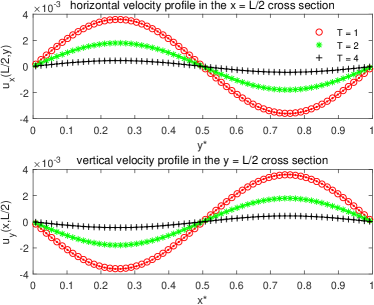
Figure 1: Numerical (symbols,resolution:$64\times 64$) and analytical (solid line) results of 2D Taylor-Green flow at different times $t=nT$ with $n=1,2,4$ and $T=ln2/(2\nu k_{1}^{2})$.

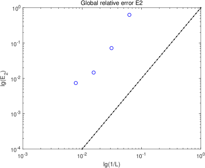
Figure 2: The convergence test: four resolutions are tested($16\times 16,32\times 32,64\times 64,128\times 128$), the solid dot line is of slope 2, the convergence order of the present scheme is almost second-order.

III.2 Womersley flow

The second numerical benchmark is the Womersley flow. In this numerical case, the flow is bounded by two parallel plate and a periodic pressure gradient or a periodic force is exerted on the flow, which results in an unsteady flow. The periodic force is $Fx(t)=-A_{p}\cos(\omega t)$, where $A_{p}$ is the amplitude and $\omega=2\pi/T$ is the frequency. Obviously, $Fx(t)$ is spatially uniform but temporally unsteady. The analytical solution of the velocity field for the Womersley flow is given by

$$U(y,t)=Re\left(i\frac{A_{p}}{\rho_{0}\omega}\left\{1-\frac{\cosh\left[(1+i)y\sqrt{\frac{\omega}{2\nu}}\right]}{\cosh\left[(1+i)L\sqrt{\frac{\omega}{2\nu}}\right]}\right\}e^{i\omega t}\right)$$ (55)

where $y\in\left[-L,L\right]$ with $2L$ being the channel width, $\nu$ is the kinematic viscosity, and $Re$ denotes the real part of the complex number.

The simulations are carried out in a computational domain with $Nx\times Ny=50\times 200$. In the $x$ direction, the periodic boundary condition is applied. The diffuse reflection boundary condition [30] is imposed on the two plates. The period $T$ is set as 1200, the kinematic viscosity is chosen as $\nu=0.1$, and the amplitude $Ap$ is set as 0.0001. The initial density is chosen as $\rho=\rho_{0}=1$. The initial flow field is static. The numerical results are obtained after running 20 periods. In Fig. 3, the velocity profile across two plates at specific times are drawn in contrast with the analytical solutions. It can be found that numerical results agree with the analytical solutions very well with the unsteady force field.

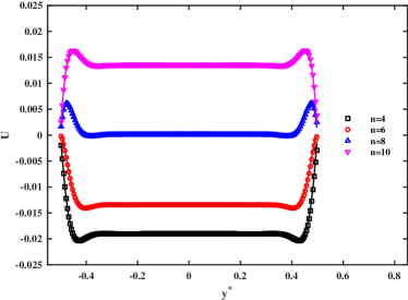
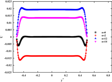
Figure 3: Numerical (symbols) and analytical (solid line) results of Womersley flow at different times $t=nT/16$ with (a) $n=4,6,8,10$ and (b) $n=0,2,12,14$.

IV Conclusions and discussions

In this work, a generic a priori derivation of the force scheme for lattice Boltzmann method based on kinetic theoretical formulation is proposed for the SMRT collision model. A second-order force scheme for the SMRT collision model is obtained and numerically verified at isothermal level. This generic approach of incorporating the force scheme actually can be applied to a wide range of collision models. At the isothermal level, we found that the force term is only not null at the first-order in the RCM space if the high-order non-equilibrium terms are ignored. The new force scheme can account for body force effects on high-order hydrodynamic moments which may be significant in flows with high density and temperature gradients, which will be reported in the following work.

Appendix A Appendix: MRT force scheme in Raw-Moment Space

In the raw-moment MRT model,the Galilean invariance and rotational invariance are not considered. For the convenient reading of this manuscript, the derivation of the force scheme of the raw-moment MRT model is stated here. Similarly, starting from Eq. (19), we can get the same evolution equation as Eq.( 24) for the MRT model in the raw-moment space. The transform of the right-hand side of Eq.( 24) to the RM space is

$$\bar{\bm{a}}_{p}^{(n)}=\bar{\bm{a}}^{(n)}-\frac{1}{\tau_{n}}(\bm{a}^{(n)}-\bm{a}^{(n)}_{0})+\bm{a}^{(n)}_{F}$$ (56)

in which the subscript p denotes the post-collision state and $\bar{\bm{a}}^{(n)}$ is the mapping of Eq. (23) in RM space

$$\bar{\bm{a}}^{(n)}=\bm{a}^{(n)}+\frac{1}{2\tau_{n}}(\bm{a}^{(n)}-\bm{a}^{(n)}_{0})-\frac{1}{2}\bm{a}^{(n)}_{F}$$ (57)

Using the above equation, Eq.( 56) can be written as the following explicit and simple moment collision equation

$$\bar{\bm{a}}_{p}^{(n)}=\bm{a}_{0}^{(n)}+(1-\frac{1}{\hat{\tau_{n}}})\bar{\bm{a}}_{1}^{(n)}+(1-\frac{1}{2\hat{\tau_{n}}})\bm{a}^{(n)}_{F},n\geq 1$$ (58)

in which $\hat{\tau_{n}}=\tau_{n}+\frac{1}{2}$, and $\bar{\bm{a}}_{1}^{(n)}=\bar{\bm{a}}^{(n)}-\bm{a}_{0}^{(n)}$.

In the numerical implementation, $\bm{a}^{(n)}_{F}=n\bm{g}\bar{\bm{a}}^{(n-1)}$. If the non-equilibrium contributions are ignored, we have

$$\bm{a}^{(1)}_{F} = \bm{F},$$ (59a)

$$\bm{a}^{(2)}_{F} = 2\bm{F}\bm{u}$$ (59b)

$$\bm{a}^{(3)}_{F} = 3\bm{F}\left[\bm{u}\bm{u}+(\theta-1)\bm{\delta}\right]$$ (59c)

$$\bm{a}^{(4)}_{F} = 4\bm{F}\left[\bm{u}\bm{u}\bm{u}+3(\theta-1)\bm{u}\bm{\delta}\right]$$ (59d)

In the RM collision operator, $\bar{\bm{a}}_{1}^{(1)}=-0.5\bm{F}$ which is indicated by Eq.( 29). $\bar{\bm{a}}_{1}^{(n)}(n=2,3)$ is obtained by the projection method. The fourth order term is obtained by the recursive approach as $\bar{\bm{a}}_{1}^{(4)}=4\bm{u}\bar{\bm{a}}_{1}^{(3)}-6\bm{u}_{1}\bar{\bm{a}}_{1}^{(2)}+4(\bm{u}\bm{u}_{2})\bar{\bm{a}}_{1}^{(1)}$. Thus the post-collision particle distribution function can be evaluated as

$$\bar{f}_{i,p} = \omega_{i}\sum_{n=0}^{4}\frac{1}{n!}\bm{a}_{0}^{(n)}:{\cal H}^{(n)}(\bm{\xi}_{i})+$$

$$\omega_{i}\sum_{n=1}^{4}\frac{1}{n!}\left\{(1-\frac{1}{\hat{\tau_{n}}})\bar{\bm{a}}_{1}^{(n)}+(1-\frac{1}{2\hat{\tau_{n}}})\bm{a}^{(n)}_{F}\right\}:{\cal H}^{(n)}(\bm{\xi}_{i})$$

Then the stream can be conducted as

$$f_{i}(\bm{x}+\bm{\xi}_{i},t+1)=\bar{f}_{i,p}(\bm{x},t).$$ (61)

References

- Bawazeer et al. [2021] S. A. Bawazeer, S. S. Baakeem, and A. A. Mohamad, Arch. Comput. Methods Eng. 28, 4405 (2021).
- Shan and Chen [1993] X. Shan and H. Chen, Phys. Rev. E 47, 1815 (1993).
- Shan and Chen [1994] X. Shan and H. Chen, Phys. Rev. E 49, 2941 (1994).
- Huang et al. [2011] H. Huang, M. Krafczyk, and X. Lu, Phys. Rev. E 84, 046710 (2011).
- Sun et al. [2012] K. Sun, T. Wang, M. Jia, and G. Xiao, Phys. A Stat. Mech. its Appl. 391, 3895 (2012).
- Guo et al. [2002] Z. Guo, C. Zheng, and B. Shi, Phys. Rev. E 65, 046308 (2002).
- Yu and Fan [2009] Z. Yu and L.-S. Fan, J. Comput. Phys. 228, 6456 (2009).
- Li et al. [2012] Q. Li, K. H. Luo, and X. J. Li, Phys. Rev. E 86, 016709 (2012).
- Kupershtokh [2004] A. L. Kupershtokh, in Proeedings 5th Int. EDH Work. (Poitiers, 2004) pp. 241–246.
- Lycett-Brown and Luo [2016] D. Lycett-Brown and K. H. Luo, Phys. Rev. E 94, 053313 (2016).
- De Rosis [2017] A. De Rosis, Phys. Rev. E 95, 023311 (2017).
- Fei and Luo [2017] L. Fei and K. H. Luo, Phys. Rev. E 96, 053307 (2017), arXiv:1705.11092 .
- Shan and He [1998] X. Shan and X. He, Phys. Rev. Lett. 80, 65 (1998).
- Shan et al. [2006] X. Shan, X.-F. Yuan, and H. Chen, J. Fluid Mech. 550, 413 (2006).
- Martys et al. [1998] N. S. Martys, X. Shan, and H. Chen, Phys. Rev. E 58, 6855 (1998).
- Shan [2019] X. Shan, Phys. Rev. E 100, 043308 (2019).
- Li et al. [2019] X. Li, Y. Shi, and X. Shan, Phys. Rev. E 100, 013301 (2019).
- Shan et al. [2021] X. Shan, X. Li, and Y. Shi, Philos. Trans. R. Soc. A Math. Phys. Eng. Sci. 379, 20200406 (2021).
- Chen and Doolen [1998] S. Chen and G. D. Doolen, Annu. Rev. Fluid Mech. 30, 329 (1998).
- He et al. [1998] X. He, S. Chen, and G. D. Doolen, J. Comput. Phys. 146, 282 (1998).
- Li and Shan [2021] X. Li and X. Shan, Phys. Rev. E 103, 043309 (2021), arXiv:2010.01476 .
- Shi and Shan [2021] Y. Shi and X. Shan, Phys. Fluids 33, 037134 (2021).
- Chapman and Cowling [1970] S. Chapman and T. G. Cowling, The Mathematical Theory of Non-uniform Gases, 3rd ed. (Cambridge University Press, 1970).
- Bhatnagar et al. [1954] P. L. Bhatnagar, E. P. Gross, and M. Krook, Phys. Rev. 94, 511 (1954).
- Huang [1987] K. Huang, Statistical Mechanics, 2nd ed. (John Wiley & Sons, New York, 1987).
- Grad [1949a] H. Grad, Commun. Pure Appl. Math. 2, 325 (1949a).
- Grad [1949b] H. Grad, Commun. Pure Appl. Math. 2, 331 (1949b).
- Malaspinas [2009] O. P. Malaspinas, Lattice Boltzmann Method for the Simulation of Viscoelastic Fluid Flows, Ph.D. thesis (2009).
- Li et al. [2022] X. Li, X. Shan, and W. Duan, ACTA AERODYNAMICA SINICA 40, 46 (2022).
- Meng and Zhang [2014] J. Meng and Y. Zhang, J. Comput. Phys. 258, 601 (2014).