Collision-free Source Seeking Control Methods for Unicycle Robots

Abstract

In this work, we propose a collision-free source-seeking control framework for unicycle robots traversing an unknown cluttered environment. In this framework, obstacle avoidance is guided by the control barrier functions (CBF) embedded in quadratic programming and the source seeking control relies solely on the use of on-board sensors that measure the signal strength of the source. To tackle the mixed relative degree of the CBF, we proposed three different CBFs, namely the zeroing control barrier functions (ZCBF), exponential control barrier functions (ECBF), and reciprocal control barrier functions (RCBF) that can directly be integrated with our recent gradient-ascent source-seeking control law. We provide rigorous analysis of the three different methods and show the efficacy of the approaches in simulations using Matlab, as well as, using a realistic dynamic environment with moving obstacles in Gazebo/ROS.

I Introduction

In the development of autonomous systems, such as autonomous vehicles, autonomous robots and autonomous spacecraft, safety-critical control systems are essential for ensuring the attainment of the control goals while guaranteeing the safe operations of the systems [3, 4]. For example, autonomous robots may need to fulfill the source-seeking task while navigating in an unknown environment safely. This capability is important for search and rescue missions and for chemical/nuclear disaster management systems. Unlike standard robotic control systems that are equipped with path-planning algorithms, the design of safe source-seeking control systems is challenging for several factors. Firstly, the source/target location is not known apriori and hence path planning cannot be done beforehand. Secondly, the lack of global information on the obstacles in an unknown environment (such as underwater, indoor or hazardous disaster area) prevents the deployment of safe navigation trajectory generation [5, 1]. Thirdly, the control systems must be able to solve these two sub-tasks consistently without generating conflicts of control action.

As another important control problem in high-tech systems and robotics, motion control with guaranteed safety has become essential for safety-critical systems. In this regard, the obstacle avoidance problem in robotics is typically rewritten as a state-constrained control problem, where collision with an obstacle is regarded as a violation of state constraints. Using this framework, multiple strategies have been proposed in the literature that can cope with static and dynamic environments. One popular obstacle avoidance algorithm is inspired by the use of the control barrier function (CBF) for nonlinear systems [29, 30, 31]. The integration of stabilization and safety control can be done either by combining the use of control Lyapunov function (CLF) with CBF as pursued in [24], or by recasting the two control objectives in the constraint of a given dynamic programming, such as the ones using quadratic programming (QP) in [32, 33]. A relaxation on the sub-level set condition in the CBF has been studied in [35, 36]. For the approach that recast the problem into QP, the early works in [34, 43] are applicable only to systems with relative-degree of one, where the relative degree is with respect to the barrier function as the output.

Another common approach of collision-free source-seeking is extremum-seeking-control (ESC) [56, 57, 58], where the potentials of the source and the obstacles are integrated into a navigation function such that the steady-state gradient of potential can be estimated. However, given the application of excitation signals for inferring the cost function, this approach can result in slow convergence and is affected by the initialization. Moreover, the repulsive potential of the obstacles is integrated into the control input at all time. As far as the authors are aware, the integration of CBF with the aforementioned source-seeking control problem has not yet been reported in the literature. In contrast to the path-planning problem where the target location is known in advance, the combination of the CBF-based method with source-seeking control is non-trivial due to the lack of information on the source location. Moreover, solving this problem for non-holonomic systems (such as unicycles) adds to the challenge, where the nominal distance-based CBF can cause a relative degree problem for the control inputs (i.e., relative degree of one with respect to longitudinal velocity input and relative degree of two with respect to the angular velocity input). Using existing methods proposed in the literature, it is not trivial to include both inputs in the CBF constraint formulated in QP. A standard solution is to linearize the unicycle by considering a virtual point instead of the robot’s center [49, 50, 51], however, it would result in an undesired offset in avoidance motion. Another solution is to achieve both tasks by solely controlling the angular velocity and maintaining a constant small linear velocity, which limits the performance of the robot in motion.

To overcome the mixed relative degree problem and provide flexibility for unicycle robot motion, we propose the collision-free source-seeking control system for the autonomous robot that is described by the unicycle system. The considered source field can represent the concentration of chemical substance/radiation in the case of chemical tracing, the heat flow in the case of hazardous fire, the flow of air or water in the case of locating a potential source, etc. The field strength is assumed to decay as the distance to the source increases. We extend our previous source-seeking control work in [23], where a projected gradient-ascent control law is used to solve the source-seeking problem, by combining it with the control barrier function (CBF) method to avoid obstacles on its path toward the source. In summary, we propose three different collision-free source-seeking control design frameworks using zeroing control barrier function (ZCBF), exponential control barrier function (ECBF) and reciprocal control barrier function (RCBF), as follows:

1. ZCBF-based approach: We solve the mixed relative degree problem by extending the state space where the longitudinal acceleration replaces the longitudinal velocity input. This enables us to construct a distance & bearing-based ZCBF that has a common relative degree of one with respect to the new inputs.

2. ECBF-based approach: In this approach, we use only the angular velocity $\omega$ to steer the system away from the obstacles while the projection gradient-ascent law [23] is still used to guide the unicycle towards the source. Consequently, we propose the use of the distance-based ECBF method as proposed in [37], which can deal with the relative degree of two with respect to the angular velocity input.

3. RCBF-based approach: We solve the mixed-relative degree problem by constructing a distance & bearing-based RCBF for controlling the angular velocity, while we still deploy the projection gradient-ascent law [23] for the longitudinal velocity input to seek the source. It leads to a control barrier function with the relative degree of one with respect to the angular velocity input.

In all of the proposed methods presented above, they use only local sensing measurements that can practically be obtained in real-time and they can be implemented numerically using any existing QP solvers. For each control design method discussed above, we analyze the asymptotic convergence and the safety properties of the closed-loop systems. As the last contribution of this work, we evaluate the efficacy of each control method numerically using Matlab, as well as, using Gazebo/ROS platform to simulate a realistic dynamic environment.

The rest of the paper is organized as follows. In Section II, we formulate the safety-guaranteed source-seeking control problem. The control integration methods and the constructions of three control barrier functions are illustrated in Section III, with rigorous stability analysis in the Appendix. Section IV shows the efficacy of the proposed theories with simulation results in a realistic virtual Matlab/Gazebo/ROS environment. The conclusions and future work are provided in Section V.

II Problem Formulation and Preliminaries

Notations. For a vector field $f:{\mathbb{R}}^{n}\to{\mathbb{R}}^{n}$ and a scalar function $h:{\mathbb{R}}^{n}\to{\mathbb{R}}$, the Lie derivative of $h$ along the vector field $f$ is denoted by $L_{f}h(x):{\mathbb{R}}^{n}\to{\mathbb{R}}$ and defined by $L_{f}h(x)=\frac{\partial h(x)}{\partial x}f(x)$. A continuous function $\alpha:(-b,a)\rightarrow(-\infty,\infty)$ is said to belong to extended class $\mathcal{K}_{e}$ for some $a,b>0$ if it is strictly increasing and $\alpha(0)=0$.

II-A Problem Formulation

For describing our safety-guaranteed source-seeking problem in a 2-D plane, let us consider a scenario where the mobile robot has to locate an unknown signal source while safely traversing across a cluttered environment. The signal strength decays with the increasing distance to the source, and the robot is tasked to search and approach the source as quickly as possible while performing active maneuvers to avoid collision with the obstacles based on the available local measurements.

Assumption II.1.

The source distribution $J(x,y)$ of the obstacle-occupied environment is a twice differentiable, radially unbounded strictly concave function in the $(x,y)$-plane with a global maximum at the source location $(x^{*},y^{*})$, e.g. $J(x^{*},y^{*})>J(x,y)$ for all $(x,y)\neq(x^{*},y^{*})$. It is assumed that the local source field signal can be measured at any free location in the obstacle-occupied environment.

Remark II.1.

The robot is equipped with an on-board sensor system and it is only able to obtain the local measurements, including the source signal, and the distance & bearing with respect to the environmental obstacles. The signal distribution function $J(x,y)$ and the positions of obstacles are both unknown apriori.

Consider a unicycle robot that is equipped with local sensors for measuring the source gradient and the distance to obstacles in the vicinity. Its dynamics is given by

$$\left[\begin{matrix}\dot{x}\\ \dot{y}\\ \dot{\theta}\end{matrix}\right]=\left[\begin{matrix}\cos(\theta)&0\\ \sin(\theta)&0\\ 0&1\end{matrix}\right]\left[\begin{matrix}v\\ \omega\end{matrix}\right],$$ (1)

where $\left[\begin{smallmatrix}x(t)&y(t)\end{smallmatrix}\right]^{\top}$ is the 2D planar robot’s position with respect to a global frame of reference and $\theta(t)$ is the heading angle. As usual, the control inputs are the longitudinal velocity input variable $v(t)$ and the angular velocity input variable $\omega(t)$.

Let us now present a general safety-guaranteed problem for general affine nonlinear systems given by

$$\dot{\xi}=f(\xi)+g(\xi)u,\quad\xi(0)=\xi_{0}\in\mathcal{X}_{0}$$ (2)

where $\xi\in{\mathcal{X}}\subset\mathbb{R}^{n}$ is the state, $u\in\mathbb{R}^{m}$ is the control input, $f(\xi):\mathbb{R}^{n}\rightarrow\mathbb{R}^{n}$ and $g(\xi):\mathbb{R}^{n}\rightarrow\mathbb{R}^{n\times m}$ are assumed to be locally Lipschitz continuous. It is assumed that the state space $\mathcal{X}$ can be decomposed into a safe set $\mathcal{X}_{s}$ and unsafe set $\mathcal{X}_{u}$, such that $\mathcal{X}_{s}\cup\mathcal{X}_{u}={\mathcal{X}}\subset\mathbb{R}^{2}$. Furthermore, we assume that the safe set $\mathcal{X}_{s}$ can be characterized by a continuously differentiable function $h:\mathbb{R}^{n}\rightarrow\mathbb{R}$ so that

$$\mathcal{X}_{s} =\left\{\xi\in{\mathcal{X}\subset}\mathbb{R}^{n}:h(\xi)\geq 0\right\}$$ (3)

$$\partial\mathcal{X}_{s} =\left\{\xi\in{\mathcal{X}\subset}\mathbb{R}^{n}:h(\xi)=0\right\}$$ (4)

$$\text{Int}(\mathcal{X}_{s}) =\left\{\xi\in{\mathcal{X}\subset}\mathbb{R}^{n}:h(\xi)>0\right\}$$ (5)

hold where $\partial\mathcal{X}_{s}$ and $\text{Int}(\mathcal{X}_{s})$ define the boundary and interior set, respectively.

Definition II.2.

(Forward invariant) The set $\mathcal{X}_{s}$ is called forward invariant for (2) if the implication $\xi_{0}\in\mathcal{X}_{s}\Rightarrow\xi(t)\in\mathcal{X}_{s}$ for all $t$ holds. Then the system (2) is safe if $\mathcal{X}_{s}$ is forward invariant.

Definition II.3.

(Relative degree, [55]) A sufficiently smooth function $h:\mathbb{R}^{n}\rightarrow\mathbb{R}$ is said to have relative degree $1\leq\rho\leq n$ with respect to the system (2) in a region $\mathcal{R}\subset\mathcal{X}$ if

1. $L_{g}L^{i-1}_{f}h(\xi)=\bm{0}_{1\times m},\,\forall 1\leq i\leq\rho-1$;

2. $L_{g}L^{\rho-1}_{f}h(\xi)\neq\bm{0}_{1\times m}$,  $\forall\xi\in\mathcal{R}$.

Definition II.4.

(Control barrier function) For the dynamical system (2), a $C^{1}$ Control Barrier Function (CBF) is a non-negative function $h:{\mathbb{R}}^{n}\to{\mathbb{R}}$ satisfying (3)-(5), and $h(x(t))$ remains positive along the trajectories of the closed-loop system (for a given control law $u=k(x)$) for all positive time. In particular, the Zeroing Control Barrier Function (ZCBF) $h$ has to satisfy

$$\sup_{u\in\mathcal{U}}[L_{f}h(\xi)+L_{g}h(\xi)u+\alpha(h(\xi))]\geq 0,$$ (6)

for all $\xi\in\mathcal{X}$, where $\mathcal{X}_{s}\subseteq\mathcal{X}\subset\mathbb{R}^{n}$ and $\alpha\in\mathcal{K}_{e}$ [33, Def. 5].

For simplicity of formulation and presentation, we assume that there is a finite number of obstacles, labeled by $\{\mathcal{O}_{1},\mathcal{O}_{2},\ldots,\mathcal{O}_{q}\}$, where $q$ is the number of obstacles and each obstacle $\mathcal{O}_{i}$ is an open bounded set in ${\mathbb{R}}^{2}$.

Safety-guaranteed source seeking control problem: Given the unicycle robotic system (1) with initial condition $\left[\begin{smallmatrix}x_{0}&y_{0}&\theta_{0}\end{smallmatrix}\right]^{\top}\in\mathcal{X}_{0}$ and with a given set of safe states $\mathcal{X}_{s}:=\Omega\times{\mathbb{R}}$ where $\Omega\subset\mathbb{R}^{2}\backslash\left(\cup_{i}\mathcal{O}_{i}\right)$ is the set of safe states in the 2D plane, design a feedback control law $v^{*},\omega^{*}$, such that

$$\lim_{t\to\infty}\left\|\left[\begin{matrix}x(t)-x^{*}\\ y(t)-y^{*}\end{matrix}\right]\right\|=0,$$ (7)

and the unicycle system is safe at all time, i.e.,

$$\left[\begin{smallmatrix}x(t)\\ y(t)\\ \theta(t)\end{smallmatrix}\right]\in\mathcal{X}_{s},\qquad\forall t\geq 0.$$ (8)

II-B Source-seeking Control with Unicycle Robot

In our recent work [23], a source-seeking control algorithm is proposed for a unicycle robot using the gradient-ascent approach. We demonstrated that the proposed controller can steer the robot towards a source, e.g. (7) holds for all initial conditions $(x(0),y(0),\theta(0))\in\mathcal{X}_{0}$, based solely on the available gradient measurement of the source field and robot’s orientation. Specifically, the control law generates longitudinal velocity ${v_{s}}=F(\nabla J(x,y),\theta)$ and angular velocity $\omega_{s}=G(\nabla J(x,y),\theta)$ as

$${u_{s}=\begin{bmatrix}v_{s}\\ \omega_{s}\end{bmatrix}}=\begin{bmatrix}k_{1}\left\langle\vec{o}(\theta),\nabla J(x,y)\right\rangle\\ -k_{2}\left\langle\vec{o}(\theta),{\nabla J^{\perp}}(x,y)\right\rangle\end{bmatrix},$$ (9)

where $\vec{o}(\theta)=\left[\begin{smallmatrix}\cos(\theta)&\sin(\theta)\end{smallmatrix}\right]$ is the robot’s unit vector orientation, the variable $\nabla J(x,y)$ is the source’s field gradient measurement, e.g., $\nabla J(x,y)=\left[\begin{smallmatrix}\frac{\partial J}{\partial x}(x,y)&\frac{\partial J}{\partial y}(x,y)\end{smallmatrix}\right]$ with $\nabla J^{\perp}$ denoting the orthogonal unit vector of $\nabla J$, and the control parameters are set as $k_{1}>0,k_{2}>0$ in the concave source field. Note that the gradient measurement $\nabla J(x,y)$ can be obtained from the local sensor system on the robot, hence apriori knowledge of the source field is not necessary in practice. We refer to our previous work [23, Section IV-B] on the local practical implementation of such source-seeking control.

III Control design and analysis

The collision-free source-seeking problem aims to design a control law using local measurements such that the unicycle robot states remain within the safe set $\mathcal{X}_{s}$ for all positive time (or, equivalently $\mathcal{X}_{s}$ is forward invariant, (8) holds) and asymptotically converge to the unknown source’s location (i.e. (7) holds). In this section, we present three CBF-based control designs that integrate our source-seeking controller (9) with the safety constraints, and mainly discuss the construction of CBFs that tackle the mixed relative degree problem.

III-A Zeroing Control Barrier Function-based Safe Source Seeking Control

Using the notations of a safe set (3)-(5) that will be incorporated in $h$, the following safe set is defined for the safety-guaranteed navigation problem of our mobile robot while seeking the source:

$$\mathcal{X}_{s}=\left\{\left[\begin{smallmatrix}x\\ y\\ \theta\end{smallmatrix}\right]\in{\mathbb{R}}^{3}\,|\,\text{dist}\left(\left[\begin{smallmatrix}x\\ y\end{smallmatrix}\right],\mathcal{O}_{i}\right)-d_{1}>0,i=1,\ldots,q\right\}$$ (10)

where dist$\left(\left[\begin{smallmatrix}x\\ y\end{smallmatrix}\right],\mathcal{O}_{i}\right)$ is the Euclidean distance of the robot position $\left[\begin{smallmatrix}x\\ y\end{smallmatrix}\right]$ to the obstacle $\mathcal{O}_{i}$ and $d_{1}\in\mathbb{R}_{+}$ is a prescribed safe distance margin around the obstacle. In other words, the safe sets are the domain outside the ball of radius $d_{1}$ around the obstacles $\mathcal{O}_{i}$. Here, we do not prescribe any specific form of the obstacle set $\mathcal{O}_{i}$, as the robot’s safety only concerns the Euclidean distance between the obstacle’s surface and its position.

The first challenge is the relative degree problem when the source-seeking control law (9) is integrated with the control barrier function for guaranteeing safe passage. The standard use of $h(x,y)$ that depends only on the distance measurement is not suitable for the unicycle-model robot (1) as it will result in a mixed relative degree system. In this case, the condition (6) leads to the situation where angular velocity input $\omega$ cannot be used to influence $h(\xi)$ since $\frac{\partial h}{\partial\xi}\left[\begin{smallmatrix}0\\ 0\\ 1\end{smallmatrix}\right]=0$.

The general solution is to apply a virtual leading point in front of the robot with the near-identity diffeomorphism [49, 50, 51], which would result in an undesired offset with respect to the robot’s actual position. To avoid the offset limitation, we tackle the mixed relative degree in the unicycle model (1) by considering an extended state space $\xi=\left[\begin{smallmatrix}x&y&v&\dot{x}&\dot{y}\end{smallmatrix}\right]^{\top}$ such that the extended dynamics is given by

$$\dot{\xi}=\left[\begin{smallmatrix}\dot{x}\\ \dot{y}\\ \dot{v}\\ \ddot{x}\\ \ddot{y}\end{smallmatrix}\right] =\left[\begin{smallmatrix}v\cos(\theta)\\ v\sin(\theta)\\ 0\\ 0\\ 0\end{smallmatrix}\right]+\left[\begin{smallmatrix}0&0\\ 0&0\\ 1&0\\ \cos(\theta)&-v\sin(\theta)\\ \sin(\theta)&v\cos(\theta)\end{smallmatrix}\right]\left[\begin{smallmatrix}a\\ \omega\end{smallmatrix}\right]$$ (11)

$$=\underbrace{\left[\begin{smallmatrix}\xi_{4}\\ \xi_{5}\\ 0\\ 0\\ 0\end{smallmatrix}\right]}_{f(\xi)}+\underbrace{\left[\begin{smallmatrix}0&0\\ 0&0\\ 1&0\\ \frac{\xi_{4}}{\xi_{3}}&-\xi_{5}\\ \frac{\xi_{5}}{\xi_{3}}&\xi_{4}\end{smallmatrix}\right]}_{g(\xi)}\underbrace{\left[\begin{smallmatrix}a\\ \omega\end{smallmatrix}\right]}_{u}$$

where $u=\left[\begin{smallmatrix}a\\ \omega\end{smallmatrix}\right]\in\mathbb{R}^{2}$ is the new control input with the longitudinal acceleration $a$ and the angular velocity $\omega$. Since we consider only the forward direction of the unicycle to solve the safety-guaranteed source seeking control problem, the state space of $\xi$ is given by $\Xi\subset{\mathbb{R}}^{2}\times(0,\infty)\times{\mathbb{R}}^{2}$ where the longitudinal velocity $\xi_{3}$ is defined on positive real. It follows that the function $f$ is globally Lipschitz in $\Xi$ and $g$ is locally Lipschitz in $\Xi$. Additionally, for this extended state space, the set $\mathcal{X}_{s}$ in (10) can be extended into

$$\mathcal{X}_{s,\text{ext}}=\left\{\xi\in\Xi\,\left|\,\text{dist}\left(\left[\begin{smallmatrix}\xi_{1}\\ \xi_{2}\end{smallmatrix}\right],\mathcal{O}_{i}\right)\right.-d_{1}>0,i=1,\ldots,q\right\}$$ (12)

Using the extended dynamics (11), a zeroing control barrier function $h(\xi)$ can be proposed which has a uniform relative degree of $1$. In particular, it is described by the new state variables $\xi$ as follows

$$h(x,y,v,\dot{x},\dot{y}) =D(x,y)e^{-P(x,y,v,\dot{x},\dot{y})}$$ (13)

$$i :=\mathop{\text{argmin}}\limits_{q}\left(\text{dist}\left(\left[\begin{smallmatrix}x\\ y\end{smallmatrix}\right],\mathcal{O}_{q}\right)\right)$$

$$D(x,y) =\text{dist}\left(\left[\begin{smallmatrix}x\\ y\end{smallmatrix}\right],\mathcal{O}_{i}\right)-d_{1}$$

$$P(x,y,v,\dot{x},\dot{y}) =\left\langle\vec{o}_{r},\vec{o}_{ro}\right\rangle+vd_{2}$$

where $\left\langle\cdot,\cdot\right\rangle$ denotes the usual inner-product operation, $\vec{o}_{r}=\left[\begin{smallmatrix}\frac{\dot{x}}{v}&\frac{\dot{y}}{v}\end{smallmatrix}\right]$ gives the unit orientation vector of robot, and $\vec{o}_{ro}$ is the unit bearing vector pointing to the closest point of the nearest obstacle as

$$\vec{o}_{ro}=\frac{\left[\begin{smallmatrix}x_{\text{obs},i}-x\\ y_{\text{obs},i}-y\end{smallmatrix}\right]}{\text{dist}\left(\left[\begin{smallmatrix}x\\ y\end{smallmatrix}\right],\mathcal{O}_{i}\right)}=\frac{\left[\begin{smallmatrix}x_{\text{obs},i}-x\\ y_{\text{obs},i}-y\end{smallmatrix}\right]}{\left\|\left[\begin{smallmatrix}x_{\text{obs},i}\\ y_{\text{obs},i}\end{smallmatrix}\right]-\left[\begin{smallmatrix}x\\ y\end{smallmatrix}\right]\right\|},$$ (14)

where $(x_{\text{obs},i},y_{\text{obs},i})$ denotes the point on the boundary of $\mathcal{O}_{i}$ that is the closest to $(x,y)$. Hence, the scalar function $D(x,y)$ is the distance to the closest obstacle with an added safe distance margin of $d_{1}\in\mathbb{R}_{+}$. The function $P$ denotes the projection of the robot’s orientation $\vec{o}_{r}$ onto the bearing vector $\vec{o}_{ro}$, and the sufficiently small $d_{2}\in\mathbb{R}_{+}$ is a directional offset constant to ensure that $\left\|L_{g}h\right\|\neq 0$ within the interior of the safe set $\mathcal{X}_{s,\text{ext}}$. Accordingly, as the robot gets closer to any obstacle, both scalar functions $D(x,y)$ and $e^{-P(x,y,v,\dot{x},\dot{y})}$ become smaller. It is equal to zero whenever $D=0$, e.g., $\text{dist}\left(\left[\begin{smallmatrix}x\\ y\end{smallmatrix}\right],\mathcal{O}_{i}\right)=d_{1}$.

Proposition III.1.

Consider the unicycle model with the extended dynamics (11) defined in $\mathcal{X}_{s,\text{ext}}$. Then the relative degree of the proposed ZCBF (13) with respect to the control input variable $a$ and $\omega$ is $1$ uniformly.

Proof.    Given the constructed ZCBF (13) with the new dynamics $\dot{\xi}=f(\xi)+g(\xi)u$ as in (11), the Lie derivative of $h(\xi)$ along the vector field $g(\xi)$ is given by

$$L_{g}h(\xi)=\frac{\partial h}{\partial\xi}g(\xi)=\begin{bmatrix}-Dd_{2}e^{-(p_{o}+vd_{2})}&D{{p}^{\prime}_{o}}e^{-(p_{o}+vd_{2})}\end{bmatrix}$$ (15)

where $p_{o}=\left\langle\vec{o}_{r},\vec{o}_{ro}\right\rangle$ describes the projection of the robot orientation $\vec{o}_{r}$ onto the unit bearing vector $\vec{o}_{ro}$ as in (13) and (14), and the notation ${p}^{\prime}_{o}=\left\langle\vec{o}_{r},\vec{o}^{\perp}_{ro}\right\rangle$ denotes the projection onto the orthogonal bearing vector $\vec{o}^{\perp}_{ro}$. It is straightforward that the $L_{g}h(\xi)=\bm{0}_{1\times 2}$ holds only when $D=0$. In other words, $\left\|L_{g}h(\xi)\right\|\neq 0$ for all $\xi\in{\mathcal{X}_{s,\text{ext}}}$. $\blacksquare$

We can now combine the source seeking control law as in (9) with the ZCBF-based safety constraint by solving the following quadratic programming (QP) problem:

$$u^{*} =\mathop{\mathrm{argmin}}\limits_{u\in\mathcal{U}}\frac{1}{2}\left\|u-{u_{\text{ref}}}\right\|^{2}$$ (16)

s.t. $$L_{f}h(\xi)+L_{g}h(\xi)u+\alpha(h(\xi))\geq 0$$ (17)

where $u_{\text{ref}}:=\left[\begin{smallmatrix}a_{s}\\ \omega_{s}\end{smallmatrix}\right]$ is the reference signal for source-seeking and it is derived from $u_{s}=\left[\begin{smallmatrix}v_{s}\\ \omega_{s}\end{smallmatrix}\right]$ in (9). Since the right-hand side of (9) is continuously differentiable, the reference acceleration signal $a_{s}$ can be derived straightforwardly by differentiating $v_{s}$. In practice, this can also be numerically computed.

The resulting control law $u^{*}$ ensures that it stays close to the reference source-seeking law while avoiding obstacles through the fulfillment of the safety constraint in (17) that amounts to having $\dot{h}(\xi)\geq-\alpha(h(\xi))$. As will be shown below in Theorem III.2, by denoting $H(\xi):=L_{f}h(\xi)+L_{g}h(\xi){u_{\text{ref}}(\xi)}\alpha(h(\xi))$, the optimal solution $u^{*}$ can be expressed analytically as

$$u^{*}(\xi)=\left\{\begin{array}[]{ll}\left[\begin{smallmatrix}\dot{v}_{s}\\ \omega_{s}\end{smallmatrix}\right]-\frac{L_{g}h(\xi)^{\top}}{\left\|L_{g}h(\xi)\right\|^{2}}H(\xi)&\text{if }H(\xi)<0\text{ and},\\ &\left\|L_{g}h(\xi)\right\|\neq 0;\\ \left[\begin{smallmatrix}\dot{v}_{s}\\ \omega_{s}\end{smallmatrix}\right]&\text{otherwise}\end{array}\right.$$ (18)

The control structure and its interconnection with the plant can be depicted in a block diagram as shown in Figure 1. Note that we use the extended system dynamics (11) for solving the mixed relative degree issue, while the computed reference control $u_{\text{ref}}$ and optimal controller $u^{*}$ are still implementable in the original state equations of the unicycle. One needs to integrate the first control input in $u^{*}$ to get the longitudinal velocity input $v^{*}(t)=\int_{0}^{t}u^{*}_{1}(\tau){\rm d}\hbox{\hskip 0.5pt}\tau$.

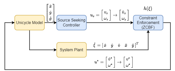
Figure 1: Block diagram of the ZCBF-based collision-free source seeking algorithm.

In the following, we will analyze the closed-loop system of the extended plant dynamics in (11) with the ZCBF-based controller, which is given by the solution of the QP problem in (16). In particular, we will provide an analytical expression of $u^{*}$, show the collision avoidance property, and finally present the asymptotic convergence to the source $\left[\begin{smallmatrix}x^{*}\\ y^{*}\end{smallmatrix}\right]$.

Theorem III.2.

Consider the extended system of a unicycle robot in $\eqref{eq:dynamics}$ with globally Lipschitz $f$ and locally Lipschitz $g$. Let the ZCBF $h$ be given as in (13) with $\mathcal{X}_{s,\text{ext}}$ as in (12) and $u_{\text{ref}}$ be derived from (9). The obstacle-occupied environment is covered by a twice-differentiable, strictly concave source field $J$ which has a unique global maximum at the source location $(x^{*},y^{*})$. Then the following properties hold:

P1.

The QP problem (16)-(17) admits a unique solution $u^{*}(\xi)$ that is locally Lipschitz in $\mathcal{X}_{s,\text{ext}}$;

P2.

The safe set $\mathcal{X}_{s,\text{ext}}$ is forward invariant, e.g., the state $\xi$ stays in safe set and $\left[\begin{smallmatrix}\xi_{1}\\ \xi_{2}\end{smallmatrix}\right]$ avoids collision with obstacles, i.e. (8) holds;

P3.

The unicycle robot asymptotically converges to the source, i.e. (7) holds.

The proof of this theorem can be found in Appendix A-A.

III-B Exponential Control Barrier Function-based Safe Source Seeking Control

In this subsection, we present another method where an exponential control barrier function (ECBF) can be directly integrated with the unicycle dynamics system (1). The collision avoidance will mainly be guided by the robot’s angular velocity. Since the unicycle robot’s motion variables (i.e. velocity $v$ and angular velocity $\omega$) are controlled independently, the sole use of angular velocity for collision avoidance will no longer pose a mixed relative degree problem. By considering the state variables $\xi=\left[\begin{smallmatrix}x\\ y\\ \theta\end{smallmatrix}\right]$ and the velocity signal $v(t)$ as an external time-varying signal, which will solely be dictated by source-seeking control law, we can rewrite the unicycle model in (1) as a time-varying affine nonlinear system as follows

$$\dot{\xi}=\underbrace{\begin{bmatrix}\cos(\xi_{3})v(t)\\ \sin(\xi_{3})v(t)\\ 0\end{bmatrix}}_{f(\xi,t)}+\underbrace{\begin{bmatrix}0\\ 0\\ 1\end{bmatrix}}_{g(\xi)}\underbrace{\omega}_{u}$$ (19)

where the angular velocity $\omega$ will be used to avoid the collision with the obstacles and $v=k_{1}\left\langle\vec{o}(\theta),\nabla J(x,y)\right\rangle$ is the source-seeking control as in (9).

For a given safe set $\mathcal{X}_{s}$, we define a distance-based barrier function $h$ that satisfies (3)-(5) as follows

$$h(\xi) =D(x,y)+(x_{\text{obs},i}-x)^{2}d_{2}+(y_{\text{obs},i}-y)^{2}d_{3},$$ (20)

where $x_{\text{obs},i}$ and $y_{\text{obs},i}$ are as in (13),

$$D(x,y)=\text{dist}\left(\left[\begin{smallmatrix}x\\ y\end{smallmatrix}\right],\mathcal{O}_{i}\right)-(d_{1}+\max\{d_{2},d_{3}\})$$ (21)

with $d_{1}>0$ be the minimum safe distance margin from the obstacle boundary $\mathcal{O}_{i}$, and the variables $d_{2},d_{3}$ be chosen sufficiently small such that $d_{2}\neq d_{3}$ and $d_{2},d_{3}<d_{1}$. As it will be clear in the main result of this subsection, the variables $d_{2}$ and $d_{3}$ are introduced to ensure that $L_{g}L_{f}h\neq 0$ so that $h$ can always be used to steer the robot away from the obstacle. Since the second and third terms of (20) affect the minima of $h$, we include $d_{2}$ and $d_{3}$ in $D$ so that the minimum of $h$ is located outside the safe distance margin from the obstacle boundary. Accordingly, the safe set $\mathcal{X}_{s}$ can be expressed as

$$\mathcal{X}_{s}=\left\{\xi\in\mathbb{R}^{3}\,\left|\,\text{dist}\left(\left[\begin{smallmatrix}\xi_{1}\\ \xi_{2}\end{smallmatrix}\right],\mathcal{O}_{i}\right)\right.-d_{1}>0,i=1,\ldots,q\right\}$$ (22)

Since $h(\xi)$ has a relative degree $k=2$ with respect to the angular velocity $\omega$, the first order Lie derivative $L_{g}h(\xi)=0$, which implies that the control input $\omega$ cannot be used in a first-order constraint set as used before in the ZCBF approach (17). Alternatively, an exponential control barrier function (ECBF)[37], which can handle state-dependent constraints for nonlinear systems with any relative degree, will be used to tackle this problem.

In order to describe ECBF, let us denote

$$\lambda=\begin{bmatrix}h(\xi)\\ \dot{h}(\xi)\end{bmatrix}=\begin{bmatrix}h(\xi)\\ L_{f}h(\xi)\end{bmatrix}.$$ (23)

Since $L_{g}L_{f}h(\xi)$ is a scalar value, we can apply feedback linearization that leads to

$$\dot{\lambda} =\begin{bmatrix}\dot{h}(\xi)\\ \ddot{h}(\xi)\end{bmatrix}=\begin{bmatrix}L_{f}h(\xi)\\ L^{2}_{f}h(\xi)+L_{g}L_{f}h(\xi)u\end{bmatrix}$$ (24)

$$=\underbrace{\begin{bmatrix}0&1\\ 0&0\end{bmatrix}}_{F}\begin{bmatrix}h(\xi)\\ L_{f}h(\xi)\end{bmatrix}+\underbrace{\begin{bmatrix}0\\ 1\end{bmatrix}}_{G}u_{k}$$

$$=F\lambda+Gu_{k}$$

$$h(\xi) =\underbrace{\begin{bmatrix}1&0\end{bmatrix}}_{C}\lambda$$

where $u_{k}:=L^{2}_{f}h(\xi)+L_{g}L_{f}h(\xi)u$ will be a new input that can be designed to ensure that $h(\xi(t))\geq 0$ for all $t\geq 0$ (i.e. the robot state remains in the safe set $\mathcal{X}_{s}$ for all positive time). Following the ECBF approach as presented in [37, Theorem 2], we can design a state feedback $-\gamma\lambda$ with $\gamma=\left[\begin{matrix}\gamma_{1}&\gamma_{2}\end{matrix}\right]$, $\gamma_{1},\gamma_{2}>0$ to define a safety constraint for $u_{k}$. By imposing $u_{k}\geq-\gamma\lambda$, it follows from (24) that

$$\dot{\lambda}\geq(F-G\gamma)\lambda.$$

In particular, the last row of the above state equation satisfies

$$\ddot{h}(\xi)\geq-\gamma_{1}h(\xi)-\gamma_{2}\dot{h}(\xi).$$

As proposed in [37, Theorem 2], one can assign $\gamma$ such that $F-G\gamma$ is Hurwitz and the constraint $u_{k}\geq-\gamma\lambda(\xi)$ ensures that $h$ is an ECBF.

As a result, by incorporating the ECBF $h(\xi)$ into the quadratic programming (QP) problem, the safety-guaranteed source seeking control problem can be realized by

$$u^{*}=\mathop{\mathrm{argmin}}\limits_{u\in\mathcal{U}}\frac{1}{2}\left\|u-\omega_{s}\right\|^{2}$$ (25)

s.t. $$L^{2}_{f}h+L_{g}L_{f}hu+\gamma_{1}h(\xi)+\gamma_{2}\dot{h}(\xi)\geq 0$$ (26)

$$\left[\begin{matrix}v_{s}\\ \omega_{s}\end{matrix}\right]=\left[\begin{matrix}k_{1}\left\langle\vec{o}(\theta),\nabla J(x,y)\right\rangle\\ -k_{2}\left\langle\vec{o}(\theta),\nabla J^{\perp}(x,y)\right\rangle\end{matrix}\right],$$ (27)

where $\lambda=\begin{bmatrix}h(\xi)&\dot{h}(\xi)\end{bmatrix}^{T}$ and $\gamma=\begin{bmatrix}\gamma_{1}&\gamma_{2}\end{bmatrix}$. Figure 2 shows the closed-loop system block diagram of the resulting safety-guaranteed source seeking control structure.

Figure 2: Block diagram of the ECBF-based collision-free source seeking algorithm.

Similar to the stability analysis in Section III-A, we will present in the following theorem an analytical solution of the piecewise angular velocity controller $u^{*}$, and subsequently prove the robot’s collision-free trajectory and its asymptotic convergence to the source $(x^{*},y^{*})$.

Theorem III.3.

Suppose that the ECBF $h(\xi)$ on $\mathcal{X}_{s}$ (22) and the source field $J$ satisfies Assumption II.1. Assume that the vector fields $f,g$ of the unicycle system $\eqref{eq:unicycle dynamics}$ and the reference control signal $\omega_{s}$ in (27) are all Lipschitz continuous. Suppose that $L_{g}L_{f}h(\xi)\neq 0$ for all $\xi\in\mathcal{X}_{s}$ (i.e. the relative degree of ECBF along the system dynamics is equal to 2) and $\gamma_{1},\gamma_{2}>0$ are chosen such that $\left[\begin{smallmatrix}0&1\\ -\gamma_{1}&-\gamma_{2}\end{smallmatrix}\right]$ has real negative eigenvalues. Then the following properties hold:

P1.

The QP problem (25) admits a unique solution $u^{*}(\xi)$ that is locally Lipschitz in the safe set $\mathcal{X}_{s}$;

P2.

The safe set $\mathcal{X}_{s}$ is forward invariant;

P3.

The closed-loop system is safe and asymptotically stable, i.e. (7) holds.

The proof of the Theorem III.3 can be found in the Appendix A-B.

III-C Reciprocal Control Barrier Function-based Safe Source Seeking

Now we present another method to solve the mixed relative degree of control inputs by constructing a distance & bearing-based reciprocal control barrier function (RCBF) using only the robot’s angular velocity constraint. The robot is again represented by the time-varying affine nonlinear system in (19) with the state variables $\left[\begin{smallmatrix}x\\ y\\ \theta\end{smallmatrix}\right]$. The input angular velocity will be given by the RCBF method to satisfy the safe set constraint, while the time-varying longitudinal velocity $v=k_{1}\left\langle\vec{o}(\theta),\nabla J(x,y)\right\rangle$ as given in the source seeking control law (9).

Let us construct the RCBF $B(\xi)$ for the same safe set (22) as defined by (3)-(5) with the continuously differentiable function $h(\xi)$. As presented in [33, Def.4], one main difference of RCBF in comparison to ZCBF is that the RCBF $B(\xi)$ grows unbounded towards the boundary of $\mathcal{X}_{s}$. To avoid the mixed-relative degree problem, the RCBF for collision avoidance is constructed by considering the distance and bearing of the robot to the closest obstacles in the following way

$$B(\xi)=\frac{1}{D(x,y)e^{P(x,y,\theta)}}$$ (28)

with the distance and orientation functions given by

$$D(x,y) =\text{dist}\left(\left[\begin{smallmatrix}x\\ y\end{smallmatrix}\right],\mathcal{O}_{i}\right)-d_{1}$$ (29)

$$P(x,y,\theta) =(\theta-\beta)d_{2},$$

where $\beta=\text{arctan}\frac{y_{\text{obs},i}-y}{x_{\text{obs},i}-x}$ is the bearing angle between the robot and the closest obstacle’s boundary. The parameter $d_{1}$ denotes the minimum safe distance and $d_{2}>0$ is a control parameter, both of which are similar to the ones defined in (13). Following [33, Corollary 1], given the RCBF $B(\xi)$, for all $\xi\in\text{Int}(\mathcal{X}_{s})$ satisfying (3)-(5), the forward invariance of $\mathcal{X}_{s}$ is guaranteed if the locally Lipschitz continuous controller $u$ satisfies

$$L_{f}B(\xi)+L_{g}B(\xi)u-\alpha_{3}(h(\xi))\leq 0$$ (30)

where $\alpha_{3}$ is a class $\mathcal{K}$ function, and $h(\xi)=\frac{1}{B(\xi)}=D(x,y)e^{P(x,y,\theta)}$. Accordingly, the RCBF-based safety-guaranteed source-seeking problem can be formulated as a quadratic programming (QP) below

$$u^{*}=\mathop{\mathrm{argmin}}\limits_{u\in\mathcal{U}}\left\|u-\omega_{s}\right\|^{2}$$ (31)

s.t. $$L_{f}B(\xi)+L_{g}B(\xi)u-\alpha_{3}(h(\xi))\leq 0$$

$$\left[\begin{matrix}v_{s}\\ \omega_{s}\end{matrix}\right]=\left[\begin{matrix}k_{1}\left\langle\vec{o}(\theta),\nabla J(x,y)\right\rangle\\ -k_{2}\left\langle\vec{o}(\theta),\nabla J^{\perp}(x,y)\right\rangle\end{matrix}\right]$$ (32)

where the last constraint ensures that the solution $u^{*}$ will be close to the source seeking controller solution $\omega_{s}$. The control block diagram utilizing the RCBF-based safe source-seeking controller is shown in Figure 3.

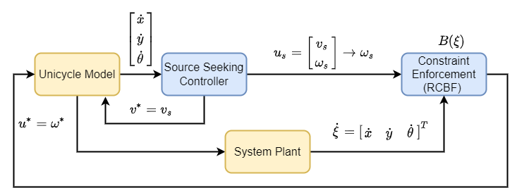
Figure 3: Block diagram of the RCBF-based collision-free source seeking algorithm.

Based on the above RCBF-based safe source seeking control using QP, we have the following theorem on the uniqueness and Lipschitz continuity of the control solution $u^{*}$, the invariant property of the safe set $\mathcal{X}_{s}$ and the asymptotic convergence towards to extremum of the source field. The proof follows similarly to that of Theorems III.2 and III.3.

Theorem III.4.

Suppose that the distance & bearing-based reciprocal control barrier function (RCBF) $B(\xi)$ in (28) with the safe set $\mathcal{X}_{s}$ in (22) and the source field $J$ satisfies Assumption II.1. Assume that the vector fields $f,g$ of the unicycle system (19), and the reference control signal $\omega_{s}$ in (32) are all Lipschitz continuous. Let $L_{g}B(\xi)\neq 0$ for all $\xi\in\mathcal{X}_{s}$ (i.e. the RCBF $B(\xi)$ has a relative degree of one with respect to the control input $\omega$). Then the following properties hold:

P1.

The QP problem (31) admits a unique solution $u^{*}(\xi)$ that is locally Lipschitz in the safe set $\mathcal{X}_{s}$;

P2.

The safe set $\mathcal{X}_{s}$ is forward invariant;

P3.

The closed-loop system is safe and asymptotically stable, i.e. (7) holds.

The proof of Theorem III.4 is presented in the Appendix A-C.

IV Simulation setup and results

In this section, we validate various methods in the previous section by using numerical simulations in Matlab and in the Gazebo/ROS environment. Firstly, we use a Matlab environment to validate the methods where static obstacles are considered. Based on these simulations, we evaluate the efficacy and generality of the approaches when they have to deal with realistic environments with dynamic obstacles by running simulations in Gazebo/ROS where multiple walking people are considered in the simulations.

IV-A Simulation Setup

In all Matlab simulations, the stationary source location $(x^{*},y^{*})$ is set at the origin $(0,0)$. Otherwise, in Gazebo/ROS simulations, we randomize the position of the source.

IV-A1 Matlab Setup

For the static obstacles, we consider multiple circular-shaped obstacles $\mathcal{O}_{i}$ with the different radii $r\in\{0.5,0.6,0.7,0.8,1.0\}$ that are set randomly around the source. Given these static obstacles and using (3)-(5), the extended safe set (12) on the extended state space $\Xi$ is given by

$$\mathcal{X}_{s,\text{ext}}=\left\{\xi\in\Xi\,\left|\,\text{dist}\left(\left[\begin{smallmatrix}\xi_{1}\\ \xi_{2}\end{smallmatrix}\right],\mathcal{O}_{i}\right)\right.>d_{1},i=1,\ldots,q\right\}$$ (33)

where $\mathcal{O}_{i}$ denotes the boundary of the $i_{th}$ obstacle, and the robot is required to maintain a minimum safe distance of $d_{1}=0.1$ with respect to the obstacles’ boundary.

For validating the performance of proposed methods in simulation, we consider a simple quadratic concave field $J(x,y)=-\left[\begin{smallmatrix}x&y\end{smallmatrix}\right]H\left[\begin{smallmatrix}x\\ y\end{smallmatrix}\right]$ where $H=H^{T}>0$. It has a unique maximum at the origin and its local gradient vector is given by $\nabla J(x,y)=-2\left[\begin{matrix}x&y\end{matrix}\right]H$.

IV-A2 Gazebo/ROS Setup

We built and performed the simulation in Gazebo/ROS (Noetic) environment which is run in Linux (Ubuntu 20.04). Figure 4 shows the common 3D room setup in the Gazebo environment where three people walk at different speeds of $0.2$ m/s, $0.4$ m/s, and $1$ m/s. These moving people are considered as dynamic obstacles by the mobile robot placed at the center of the room in this figure. The source field is given by a quadratic field and is illustrated as colored rings in Figure 4. The center for the source field is set randomly in every simulation. We note that the source distribution model is not known apriori in practical applications, and the gradient $\nabla J(x,y)$ can be estimated by local sensor systems on the robot as demonstrated in our previous work [23, Section IV-B].

The unicycle robot was simulated by the turtlebot3 (Waffle) as shown in Figure 5. The real-time distance measurement was done using the on-board $360^{\circ}$ laser distance sensor of LDS-01. The angle and distance measurement uses the sampling of $0.5^{\circ}$, i.e. $720$ samples for the whole field-of-view of $360^{\circ}$. Different from the Matlab simulation, the robot obtains the Euclidean distance between the obstacles’ boundary and its position by laser measurements. Taking into account the dynamic environment due to the movement of people in the room, the minimum safe distance between robot and any potential collisions (walls and pedestrians) is set to be $d_{1}=0.3m$ in the formulation of safe set $\mathcal{X}_{s,\text{ext}}$ in (12) or in (22).

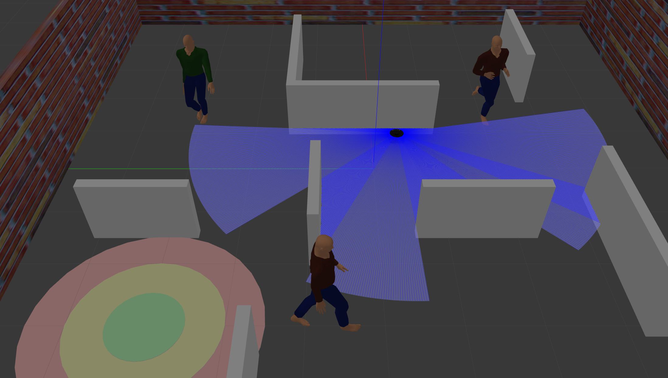
Figure 4: Laser-embedded turtlebot3 robot in the constructed gazebo world, which contains fixed walls and walking people as potential collisions for robot navigation. The center point of the green circle area stands for the source location.

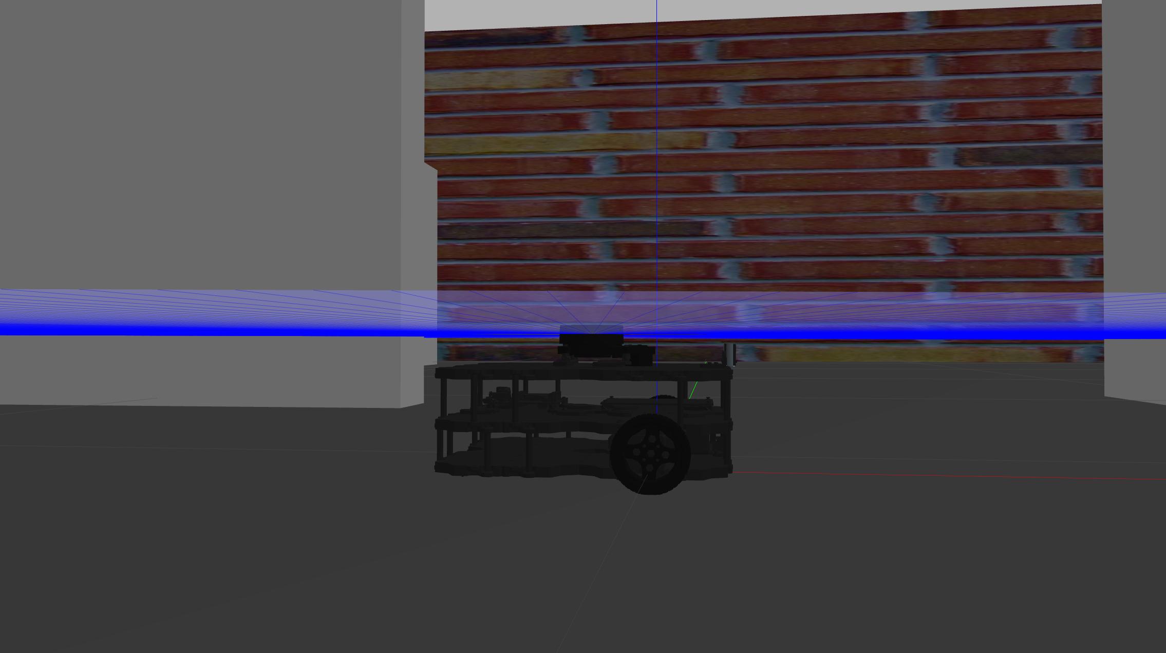
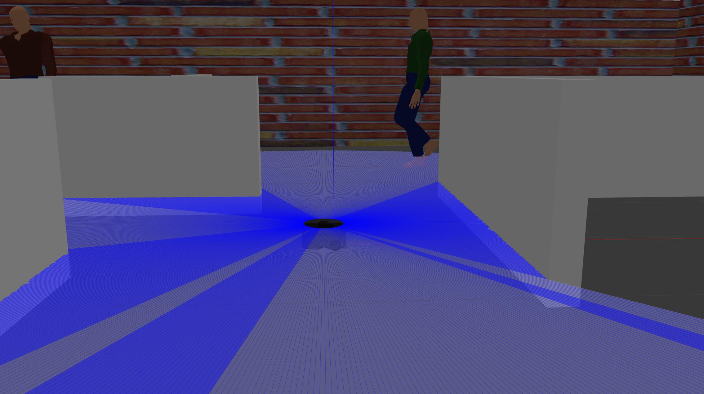
Figure 5: Laser-embedded turtlebot3 robot in the Gazebo/ROS world.

IV-B Simulation Results in Matlab

IV-B1 ZCBF-based Collision-free Source-seeking

Algorithm 1 ZCBF-based Collision-free Source-seeking

1:

2:$I$: Total time horizon

3:$d_{t}$: Sample time

4:$i=\frac{I}{d_{t}}$: Time step index

5:$\nabla J(\xi)$: Source signal gradient

6:$\vec{o}_{r},\vec{o}_{ro},\text{dist}(t)$: Orientation of robot, real-time unite-bearing and distance between the robot and the closest obstacle

7:Optimal safe control input $u^{*}=\left[\begin{smallmatrix}v^{*}\\ \omega^{*}\end{smallmatrix}\right]$

8:Initialization:

9:Set initial time step index: $i\leftarrow 0$

10:Set initial robot state: $\xi(0)=\begin{bmatrix}x_{0}&y_{0}&v_{0}&\dot{x}_{0}&\dot{y}_{0}\end{bmatrix}^{T}$

11:Pre-set source seeking control variables $k_{1},k_{2}$

12:while $i\in\left[0,I\right]$ do

13:     Source Seeking Algorithm:

14:     $u_{s}=\left[\begin{smallmatrix}v_{s}\\ \omega_{s}\end{smallmatrix}\right]\leftarrow$ Source signal measurement

15:     $\left[\begin{smallmatrix}\dot{v}_{s}\\ \omega_{s}\end{smallmatrix}\right]\stackrel{{\scriptstyle d_{t}}}{{\longleftarrow}}\left[\begin{smallmatrix}v_{s}\\ \omega_{s}\end{smallmatrix}\right]$

16:     Zeroing Control Barrier Function Constraint:

17:     $\vec{o}_{r},\vec{o}_{ro},\text{dist}(t)\leftarrow$ On-board laser/lidar measurements (considering coordinate transformation between sensor-frame and robot-frame)

18:     ZCBF constraint: $\dot{h}(\xi)\leftarrow\vec{o}_{r},\vec{o}_{ro},\text{dist}(t),\left[\begin{smallmatrix}\dot{v}_{s}\\ \omega_{s}\end{smallmatrix}\right]$

19:     Quadratic programming for optimal safe control input $u^{*}$ : QP $\leftarrow\left[\begin{smallmatrix}\dot{v}_{s}\\ \omega_{s}\end{smallmatrix}\right]$

20:     Unicycle Model Control variable transformation:

21:     $\left[\begin{smallmatrix}v^{*}\\ \omega^{*}\end{smallmatrix}\right]\leftarrow u^{*}=\left[\begin{smallmatrix}\dot{v}^{*}\\ \omega^{*}\end{smallmatrix}\right]$

22:     Apply optimal controller $\left[\begin{smallmatrix}v^{*}\\ \omega^{*}\end{smallmatrix}\right]$ to robot for a sample time $d_{t}$, and update new robot state: $\dot{\xi}\leftarrow\dot{\xi}_{\text{new}}$.

23:      Update time step:

24:     $i\leftarrow i+1$

25:end while

Algorithm 1 summarizes the ZCBF-based collision-free source-seeking which we will use to steer the unicycle robot towards the maximum of $J$ while navigating itself in the cluttered unknown environment. In the simulation, the source gradient and distance to the obstacles are observed by the robot in real time for the computation of ZCBF-based control input.

For numerical simulation purposes, we consider two different quadratic functions as given before with $H=I$ and with $H=\left[\begin{smallmatrix}5&4\\ 4&5\end{smallmatrix}\right]$. Note again the real-time reference input $u_{\text{ref}}$ for the source-seeking is derived from the projected gradient-ascent control law (9)

$$u_{s} =\begin{bmatrix}v_{s}\\ \omega_{s}\end{bmatrix}=\begin{bmatrix}k_{1}\left\langle\vec{o}(\xi_{3},\xi_{4},\xi_{5}),\nabla J(\xi_{1},\xi_{2})\right\rangle\\ -k_{2}\left\langle\vec{o}(\xi_{3},\xi_{4},\xi_{5}),\nabla J^{\perp}(\xi_{1},\xi_{2})\right\rangle\end{bmatrix}$$ (34)

where the control parameters $k_{1},k_{2}>0$, and the robot orientation $\vec{o}=\left[\begin{smallmatrix}\frac{\xi_{4}}{\xi_{3}}&\frac{\xi_{5}}{\xi_{3}}\end{smallmatrix}\right]^{T}$.

As the first control input in (11) refers to the longitudinal acceleration, instead of the usual longitudinal velocity in the unicycle model, we use the following Euler approximation to get the longitudinal velocity input from the computed longitudinal acceleration input $a(t)$ in the discrete-time numerical simulation $v_{s}(t_{k+1})=v_{s}(t_{k})+d_{t}a(t_{k})$, where $t_{k}$ and $t_{k+1}$ denote the current and next discrete-time step, respectively, and $d_{t}$ is the integration time step.

We set up a 2D simulation environment given by $[-4,4]\times[-4,4]$ with $10$ circular obstacles of different radii and centroid positions. Figure 6 shows four simulation results using the same environment, where the robot is initialized in four random initial conditions

$$\left[\begin{matrix}x_{0}\\ y_{0}\\ v_{0}\\ \dot{x}_{0}\\ \dot{y}_{0}\end{matrix}\right]\in\left\{\left[\begin{matrix}4\\ 2\\ \frac{1}{2}\\ -\frac{1}{4}\\ \frac{\sqrt{3}}{4}\end{matrix}\right],\left[\begin{matrix}-3\\ 2\\ 1\\ \frac{\sqrt{3}}{2}\\ \frac{1}{2}\end{matrix}\right],\left[\begin{matrix}-4\\ -4\\ \frac{3}{2}\\ -\frac{3\sqrt{3}}{4}\\ -\frac{3\sqrt{3}}{4}\end{matrix}\right],\left[\begin{matrix}4\\ 0\\ 2\\ 0\\ 2\end{matrix}\right]\right\}.$$

The color gradient shows the source field, where Sub-figures 6(a) and (b) are based on $H=I$, and the rest is based on $H=\left[\begin{smallmatrix}5&4\\ 4&5\end{smallmatrix}\right]$. For defining the ZCBF, the minimum safe distance between robot and the obstacle’s boundary is set to be $d_{1}=0.1$, and the parameters of reference source-seeking input control are set as $k_{1}=2,k_{2}=10$ for the first two cases when $H=I$ (c.f. the simulation results in Sub-figures 6(a) and (b)) and $k_{1}=1,k_{2}=20$ for the other cases shown in Sub-figures 6(c) and (d). These simulation results show that the unicycle is able to maneuver around the obstacles of different dimensions and to converge to the maximum point, as expected.

\includegraphics[width=433.62pt]{fig/matlab/zcbf/quad_circle/2.eps}

\includegraphics[width=433.62pt]{fig/matlab/zcbf/quad_circle/1.eps}

\includegraphics[width=433.62pt]{fig/matlab/zcbf/quad_ellipse/3.eps}

(a)

\includegraphics[width=433.62pt]{fig/matlab/zcbf/quad_ellipse/4.eps}

Figure 6: Simulation results based on the zeroing barrier function $h(x,y,v,\dot{x},\dot{y})=D(x,y)e^{-P(x,y,v,\dot{x},\dot{y})}$, where both the longitudinal and angular velocity are given by the optimal solution of ZCBF-QP (16). The source is set at the origin $(0,0)$, surrounded by multiple circular-shape obstacles, and the signal strength is distributed in the field: $(a,b):J_{1}(x,y)=-x^{2}-y^{2}$; $(c,d):J_{2}(x,y)=-5x^{2}-8xy-5y^{2}$, respectively. The robot is set at various initial positions (given by $\circ$) to search the source while avoiding any potential collisions.

IV-B2 ECBF-based Collision-free Source-seeking

Algorithm 2 ECBF-based Collision-free Source-seeking

1:

2:$I$: Total time horizon

3:$d_{t}$: Sample time

4:$i=\frac{I}{d_{t}}$: Time step index

5:$\nabla J(\xi)$: Signal gradient

6:$\text{dist}(t)$: Real-time distance between robot and obstacle

7:Optimal safe control input $u^{*}$

8:Initialization:

9:Set initial time-step: $i\leftarrow 0$

10:Set initial robot state: $\xi(0)=\begin{bmatrix}x_{0}&y_{0}&\theta_{0}\end{bmatrix}^{T}$

11:Pre-set source-seeking variables $k_{1},k_{2}$

12:while $i\in\left[0,I\right]$ do

13:     Source Seeking Algorithm:

14:     $u_{s}=\left[\begin{smallmatrix}v_{s}\\ \omega_{s}\end{smallmatrix}\right]\leftarrow$ Source signal measurement

15:     $f(\xi)=\left[\begin{smallmatrix}\cos(\xi_{3})\\ \sin(\xi_{3})\\ 0\end{smallmatrix}\right]v_{s},\omega_{s}\leftarrow\omega_{s}$.

16:     Exponential Control Barrier Function Constraint:

17:     $\text{dist}(t)\leftarrow$ On-board laser/lidar measurements (considering coordinate transformation between sensor-frame and robot-frame)

18:     ECBF constraint: $\dot{h}(\xi),\ddot{h}(\xi)\leftarrow\text{dist}(t),\omega_{s}$

19:     Quadratic programming for optimal control input $u^{*}=\omega^{*}$ : QP $\leftarrow\omega_{s}$

20:     Unicycle Model Application:

21:     Apply optimal safe control input $\left[\begin{smallmatrix}v_{s}\\ \omega^{*}\end{smallmatrix}\right]$ to robot for a sample time $d_{t}$, and update new robot state: $\dot{\xi}\leftarrow\dot{\xi}_{\text{new}}$.

22:      Update time step:

23:     $i\leftarrow i+1$

24:end while

In this part, we evaluate the performance of the ECBF-based collision-free source-seeking method that is summarized in Algorithm 2. While the computation of source-seeking reference input $v_{s}$ and $\omega_{s}$ can be done in real-time based on the local gradient information, the computation of ECBF QP problem is performed at every simulation discrete-time step. The source-seeking reference input of the unicycle dynamics (19) is given by

$$u_{s} =\begin{bmatrix}v_{s}\\ \omega_{s}\end{bmatrix}=\begin{bmatrix}k_{1}\left\langle\vec{o}(\xi_{3}),\nabla J(\xi_{1},\xi_{2})\right\rangle\\ -k_{2}\left\langle\vec{o}(\xi_{3}),\nabla J^{\perp}(\xi_{1},\xi_{2})\right\rangle\end{bmatrix},$$ (35)

where the robot orientation is expressed with the unicycle model $\vec{o}=\left[\begin{smallmatrix}\cos(\xi_{3})\\ \sin(\xi_{3})\end{smallmatrix}\right]$, and the angular velocity variable $\omega_{s}$ becomes a reference signal in the ECBF-QP problem.

Based on the same 2D environment simulation setup, we design the ECBF using the minimum safe distance $d_{1}=0.1m$ and set the parameters $\gamma_{1}=2$ and $\gamma_{2}=3$ to guarantee the forward invariance of safe set $\mathcal{X}_{s}$. For the first case of source field with $H=I$, the source-seeking control parameters are set as $k_{1}=1,k_{2}=50$, and for the other case with $H=\left[\begin{smallmatrix}5&4\\ 4&5\end{smallmatrix}\right]$, we set $k_{1}=0.2,k_{2}=40$. Subsequently, we performed four simulations with four random initial states

$$\left[\begin{matrix}x_{0}\\ y_{0}\\ \theta_{0}\end{matrix}\right]\in\left\{\left[\begin{matrix}4\\ 4\\ 60^{\circ}\end{matrix}\right],\left[\begin{matrix}-4\\ 1\\ 30^{\circ}\end{matrix}\right],\left[\begin{matrix}-2\\ -4\\ 45^{\circ}\end{matrix}\right],\left[\begin{matrix}2\\ -4\\ 90^{\circ}\end{matrix}\right]\right\},$$

and with two different source fields. The results are shown in Figure 7, where all robots are able to converge to the source and successfully avoid the obstacles.

\includegraphics[width=433.62pt]{fig/matlab/ecbf/quad_circle/2.eps}

\includegraphics[width=433.62pt]{fig/matlab/ecbf/quad_circle/1.eps}

\includegraphics[width=433.62pt]{fig/matlab/ecbf/quad_ellipse/3.eps}

(a)

\includegraphics[width=433.62pt]{fig/matlab/ecbf/quad_ellipse/4.eps}

(b)

Figure 7: Simulation results based on the exponential barrier function $h(x,y)=D(x,y)+(x_{\text{obs},i}-x)^{2}d_{2}+(y_{\text{obs},i}-y)^{2}d_{3}$, where the longitudinal and angular velocity are controlled by the projected gradient-ascent law (9) and the ECBF-based constraint (25), respectively. The source fields are depicted in $(a,b):J(x,y)=-x^{2}-y^{2}$; $(c,d):J_{2}(x,y)=-5x^{2}-8xy-5y^{2}$ where both of the sources are located at the origin $(0,0)$ surrounding by multiple circular-shape obstacles. The robot is set at four different initial states (shown as $\circ$) and traverses across all the potential collisions to search the source.

IV-B3 RCBF-based Collision-free Source-seeking

Algorithm 3 RCBF-based Collision-free Source-seeking

1:

2:$I$: Total time horizon

3:$d_{t}$: Sample time

4:$i=\frac{I}{d_{t}}$: Time step index

5:$\nabla J(\xi)$: Source signal gradient

6:$\beta(t),\text{dist}(t)$: Real-time bearing angle and distance between robot and obstacle

7:Optimal safe control input $\omega^{*}$

8:Initialization:

9:Set initial time-step: $i\leftarrow 0$

10:Set initial robot state: $\xi(0)=\begin{bmatrix}x_{0}&y_{0}&\theta_{0}\end{bmatrix}^{T}$

11:Pre-set source-seeking variables $k_{1},k_{2}$

12:while $i\in\left[0,I\right]$ do

13:     Source Seeking Algorithm:

14:     $u_{s}=\left[\begin{smallmatrix}v_{s}\\ \omega_{s}\end{smallmatrix}\right]\leftarrow$ Source signal measurement

15:     $f(\xi)=\left[\begin{smallmatrix}\cos(\xi_{3})\\ \sin(\xi_{3})\\ 0\end{smallmatrix}\right]v_{s},\omega_{s}\leftarrow\omega_{s}$.

16:     Reciprocal Control Barrier Function Constraint:

17:     $\beta(t),\text{dist}(t)\leftarrow$ On-board laser/lidar measurements (considering coordinate transformation between sensor-frame and robot-frame)

18:     RCBF constraint: $\dot{B}(\xi)\leftarrow\beta(t),\text{dist}(t),\omega_{s}$

19:     Quadratic programming for optimal safe control input $u^{*}=\omega^{*}$ : QP $\leftarrow\omega_{s}$

20:     Unicycle Model Application:

21:     Apply optimal safe controller $\left[\begin{smallmatrix}v_{s}\\ \omega^{*}\end{smallmatrix}\right]$ to robot for a time step of $d_{t}$, and update new robot state : $\dot{\xi}\leftarrow\dot{\xi}_{\text{new}}$.

22:      Update time step:

23:     $i\leftarrow i+1$

24:end while

In this subsection, we evaluate the performance of the RCBF-based safety-guaranteed source-seeking method as summarized in Algorithm 3. The time-varying longitudinal velocity $v:=v_{s}$ is guided by (32), and the QP problem in (31) is solved numerically to render the angular velocity input $\omega^{*}_{s}$. For the reference source-seeking control $\left[\begin{smallmatrix}v_{s}\\ \omega_{s}\end{smallmatrix}\right]$ in (32) along with the unicycle’s orientation vector $\vec{o}=\left[\begin{smallmatrix}\cos(\xi_{3})\\ \sin(\xi_{3})\end{smallmatrix}\right]$, we set the parameters as follows: $k_{1}=2,k_{2}=60$ for the first case with $H=I$; and $k_{1}=0.3,k_{2}=20$ for the other case with $H=\left[\begin{smallmatrix}5&4\\ 4&5\end{smallmatrix}\right]$. The simulation results are shown in Figure 8 where all the trajectories converge to the source position $(0,0)$ without any collisions.

\includegraphics[width=433.62pt]{fig/matlab/rcbf/quad_circle/2.eps}

\includegraphics[width=433.62pt]{fig/matlab/rcbf/quad_ellipse/3_new.eps}

Figure 8: Simulation results based on the reciprocal barrier function $B(x,y,\theta)=\frac{1}{D(x,y)e^{P(x,y,\theta)}}$, where the longitudinal velocity is controlled by the projected gradient-ascent law (9) and the angular velocity is derived from the solution of RCBF-based QP (31). The control method is implemented in two concave source fields as $(a):J(x,y)=-x^{2}-y^{2}$; $(b):J_{2}(x,y)=-5x^{2}-8xy-5y^{2}$ where both of the sources are located at the origin $(0,0)$ surrounding by multiple circular-shape obstacles. The robot starts from various initial states indicated by $\circ$.

IV-B4 Comparison of Methods

In this subsection, we will compare the performance of all three proposed control barrier functions, using the same parameters for the reference source seeking control: $k_{1}=0.3,k_{2}=30$. For each method (ZCBF, ECBF or RCBF-based collision-free source-seeking), we run a Monte Carlo simulation of $50$ runs, where on each run, the three methods start from the same randomized initial conditions. The resulting trajectories of the closed-loop systems are recorded and analyzed for comparing the methods. In Figure 9, we present the box plot drawn from the samples of convergence time and minimum distance to the boundary of the obstacles. The variable $T_{c}$ in Figure 9(a) refers to the convergence time for the robot to reach the final $20\%$ of the distance between the source and its initial position. The variable $D_{c}$ in Figure 9(b) represents the closest distance between the robot and the obstacle’s boundary during the maneuver towards the source point. The Monte Carlo simulation results validate the convergence analysis of all three proposed collision-free source-seeking control algorithms where the robot remains safe for all time and they are within the minimum safety margin. While all three methods perform equally well in avoiding the obstacles, the ZCBF-based method outperforms the other two approaches in both the convergence time as well as in ensuring that the safe margin of $0.1$ from the obstacles’ boundary is not trespassed. We remark that the ECBF-based and RCBF-based methods may still enter the safe margin briefly due to the discrete-time implementation of the algorithms. This robustness of the algorithms with respect to the disturbance introduced by time-discretization shows a property of input-to-state safety of the closed-loop systems as studied recently in [25, 26].

\includegraphics[width=433.62pt]{fig/matlab/box/3/T_c.eps}

\includegraphics[width=433.62pt]{fig/matlab/box/3/D_c.eps}

Figure 9: Box plot of the Monte Carlo simulation of the three control barrier function-based methods using the same reference source-seeking control parameters ($k_{1}=0.3,k_{2}=30$). The robot is initialized at $50$ random initial positions for each group of simulations.

IV-C Simulation Results in Gazebo/ROS

Using the Gazebo/ROS setup as presented in Subsection IV-A2, we evaluate the efficacy and performance of all three CBF methods in a realistic simulated environment. We emphasize that only local measurements (e.g., local signal gradient, distance, and bearing angle between the robot and the closest obstacles) are used by the robot to implement all three collision-free source-seeking navigation methods. In particular, the global information, such as, the source field function, the location of the source, the robot or the obstacles) is not relayed to the robot. The embedded laser distance sensor of LDS-01 detects all obstacles within the neighborhood of $0.12\sim 3.5m$. Based on this measurement, the bearing angle to the closest obstacle can be calculated from the $720$ samples of $360^{\circ}$ field-of-view.

Figures 10–11 show the plots of the initial and final states of the robot for each of the three CBFs-based safe source-seeking methods. The animated motion of the robot in Gazebo/ROS performing the source-seeking while avoiding these dynamic obstacles can be found in the accompanying video at. In all these realistic simulations, the three proposed methods are able to successfully reach the source and to navigate themselves in the unknown dynamic environment.

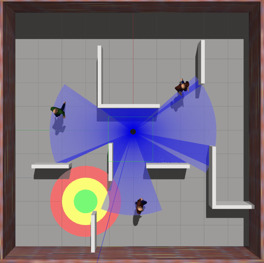
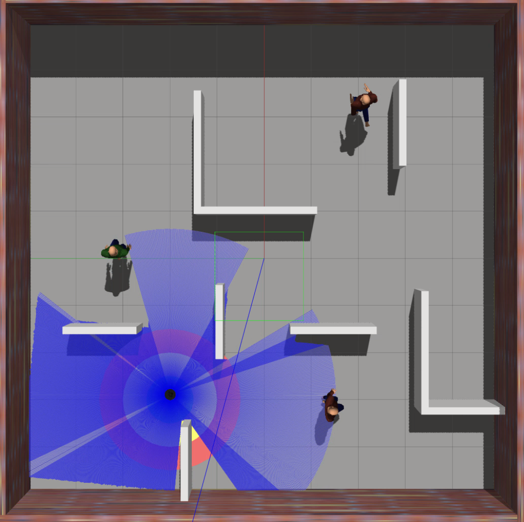
Figure 10: Simulation of the zeroing control barrier function (ZCBF)-based collision-free source-seeking in the unknown environment. Three pedestrians are walking around as dynamic obstacles. Robot is initialized with the state $(0,0,\frac{1}{2},\frac{\sqrt{2}}{4},\frac{\sqrt{2}}{4})$ in 10, and eventually arrived at the source $(-3,2)$ in 10. The source-seeking control parameters in the field $J(x,y)=-(x+3)^{2}-(y-2)^{2}$ are set as $k_{1}=0.2,k_{2}=0.5$.

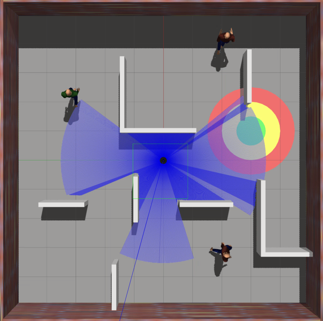
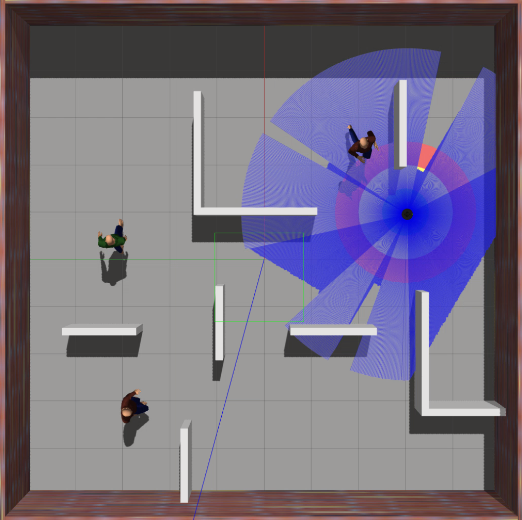
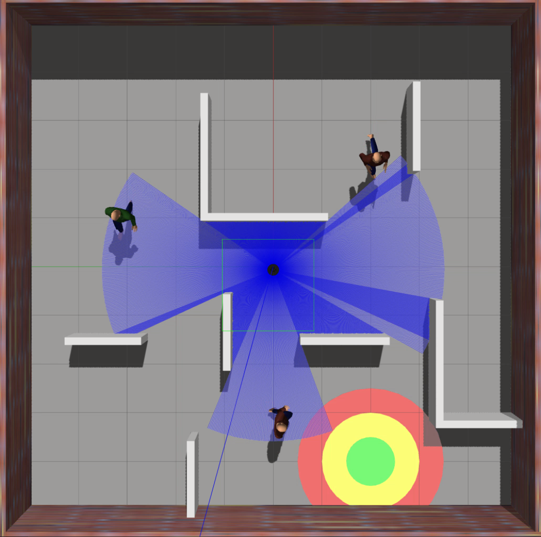
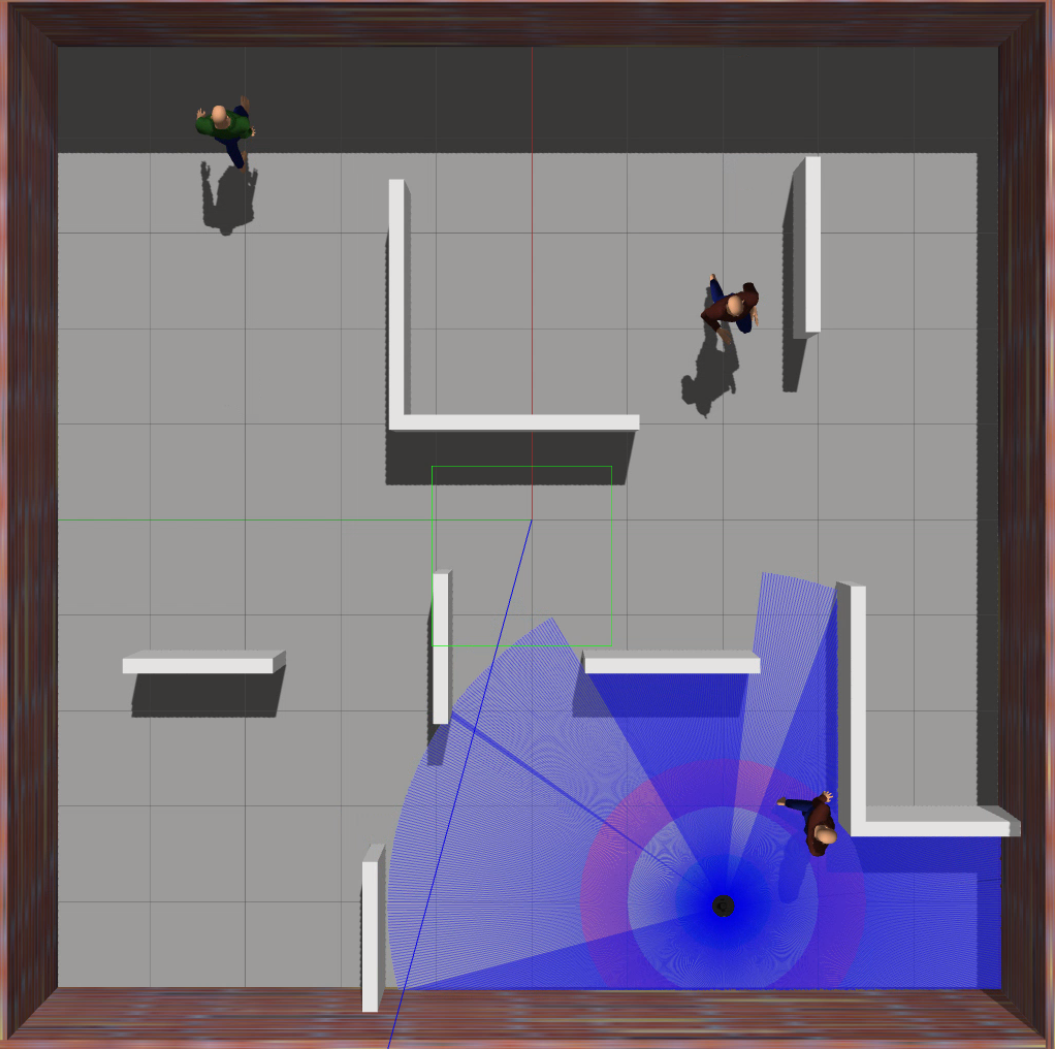
Figure 11: Simulation of collision-free source-seeking in the unknown environment with exponential control barrier function (ECBF) in 11 and 11, and reciprocal control barrier function (RCBF) in 11 and 11.Three pedestrians are walking around as dynamic obstacles. With the pre-set source-seeking parameters $k_{1}=0.2,k_{2}=0.4$ in the field $J(x,y)=-(x-1)^{2}-(x+3)^{2}$, robot is initialized with the state $(0,0,\frac{\pi}{4})$ in 11, and eventually arrived at the source $(1,-3)$ in 11 with ECBF. For RCBF validation, robot is initialized with the state $(0,0,\frac{\pi}{4})$ in 11, and eventually arrived at the source $(-4,-2)$ in 11. The source-seeking control parameters in the field $J(x,y)=-(x+4)^{2}-(y+2)^{2}$ are $k_{1}=0.2,k_{2}=0.5$.

V Conclusion

In this paper, we presented a framework of the safety-guaranteed autonomous source-seeking control for a nonholonomic unicycle robot in an unknown cluttered dynamic environment. Three different constructions of control barrier functions (ZCBF, ECBF, RCBF) are proposed to tackle the mixed relative degree problem of the unicycle’s nonholonomic constraint. Guided by the projected gradient-ascent control law as the reference control signal, we show that all three proposed control barrier function-based QP methods give locally Lipschitz optimal safe source-seeking control inputs. The analysis on safe navigation and on the convergence to the source are presented for each proposed method. The efficacy of the methods is evaluated numerically in Matlab, as well as, in Gazebo/ROS which provides a realistic simulation environment.

Appendix A Appendix

A-A Proof of Theorem III.2

Proof.    We will first prove the property P1. Let us rewrite (16)-(17) into the following QP terms of a shifted decision variable $e=u-u_{\text{ref}}\in\mathbb{R}^{2\times 1}$ with $u_{\text{ref}}=\left[\begin{smallmatrix}a_{s}\\ \omega_{s}\end{smallmatrix}\right]=\left[\begin{smallmatrix}\dot{v}_{s}\\ \omega_{s}\end{smallmatrix}\right]$ as follows

$$\qquad\qquad e^{*}=\mathop{\mathrm{argmin}}\limits_{u\in\mathcal{U}}\frac{1}{2}e^{\top}e$$ (36)

s.t. $$L_{f}h(\xi)+L_{g}h(\xi)\left(e+\left[\begin{smallmatrix}\dot{v}_{s}\\ \omega_{s}\end{smallmatrix}\right]\right)+\alpha(h(\xi))\geq 0$$ (37)

Correspondingly, define a Lagrangian function $L$ that incorporates the constraint (37) by a Lagrange multiplier $\lambda$ as follows

$$L(e,\lambda)=\frac{1}{2}e^{\top}e-\lambda\left(L_{f}h(\xi)+L_{g}h(\xi)\left(e+\left[\begin{smallmatrix}\dot{v}_{s}\\ \omega_{s}\end{smallmatrix}\right]\right)+\alpha(h(\xi))\right)$$ (38)

This QP problem for optimal safe control can be solved through the following Karush–Kuhn–Tucker (KKT) optimality conditions

$$\left.\begin{matrix}\begin{aligned} \frac{\partial L(e^{*},\lambda^{*})}{\partial e^{*}}={e^{*}}^{\top}-\lambda^{*}L_{g}h(\xi)=\left[\begin{smallmatrix}0&0\end{smallmatrix}\right]&\\ \lambda^{*}\left(L_{f}h(\xi)+L_{g}h(\xi)\left(e^{*}+\left[\begin{smallmatrix}\dot{v}_{s}&\\ \omega_{s}\end{smallmatrix}\right]\right)+\alpha(h(\xi))\right)=0&\\ L_{f}h(\xi)+L_{g}h\left(\xi)\left(e^{*}+\left[\begin{smallmatrix}\dot{v}_{s}&\\ \omega_{s}\end{smallmatrix}\right]\right)+\alpha(h(\xi)\right)\geq 0&\\ \lambda^{*}\geq 0\end{aligned}\end{matrix}\right\}$$ (39)

Based on the property of Lagrange multiplier $\lambda^{*}\geq 0$ and (39), we derived the optimal solution $u^{*}$ (as well as $e^{*}$) in the following two cases: when $\lambda^{*}>0$ (i.e., $\lambda^{*}\neq 0$), or $\lambda^{*}=0$. For convenience, let us define

$$H(\xi):=L_{f}h(\xi)+L_{g}h(\xi)\left[\begin{smallmatrix}\dot{v}_{s}\\ \omega_{s}\end{smallmatrix}\right]+\alpha(h(\xi)).$$ (40)

Case-1: $\lambda^{*}=0$. From the first condition in (39) and with $\lambda^{*}=0$, it is clear that $e^{*}=\lambda^{*}L_{g}h(\xi)^{\top}=\left[\begin{smallmatrix}0\\ 0\end{smallmatrix}\right]$. By the definition of $e$, this implies that $\left[\begin{smallmatrix}0\\ 0\end{smallmatrix}\right]=e^{*}=u^{*}-\left[\begin{smallmatrix}\dot{v}_{s}\\ \omega_{s}\end{smallmatrix}\right]$, i.e., $u^{*}=\left[\begin{smallmatrix}\dot{v}_{s}\\ \omega_{s}\end{smallmatrix}\right]=u_{\text{ref}}$ holds. By substituting $e^{*}=\left[\begin{smallmatrix}0\\ 0\end{smallmatrix}\right]$ to the third condition of (39), we obtain that

$$L_{f}h(\xi)+L_{g}h\left(\xi)\left[\begin{smallmatrix}\dot{v}_{s}\\ \omega_{s}\end{smallmatrix}\right]+\alpha(h(\xi)\right)\geq 0$$ (41)

or in other words, $H(\xi)\geq 0$ holds.

Case-2: $\lambda^{*}>0$. In order to satisfy the second condition in (39) for $\lambda^{*}>0$, it follows that

$$L_{f}h(\xi)+L_{g}h(\xi)\left(e^{*}+\left[\begin{smallmatrix}\dot{v}_{s}\\ \omega_{s}\end{smallmatrix}\right]\right)+\alpha(h(\xi)=0$$ (42)

By substituting the solution of the first condition in (39) with $e^{*}=\lambda^{*}L_{g}h(\xi)^{\top}$ to the above equation, we get

$$L_{f}h(\xi)+L_{g}h(\xi)\left(\lambda^{*}L_{g}h(\xi)^{\top}+\left[\begin{smallmatrix}\dot{v}_{s}\\ \omega_{s}\end{smallmatrix}\right]\right)+\alpha(h(\xi))=0.$$ (43)

Accordingly, the Lagrange multiplier $\lambda^{*}$ can be expressed as

$$\lambda^{*}=-\frac{L_{g}h(\xi)\left[\begin{smallmatrix}\dot{v}_{s}\\ \omega_{s}\end{smallmatrix}\right]+L_{f}h(\xi)+\alpha(h(\xi))}{L_{g}h(\xi)L_{g}h(\xi)^{\top}},$$ (44)

where $L_{g}h(\xi)L_{g}h(\xi)^{\top}$ is scalar. Therefore, the optimal $e^{*}$ and $u^{*}$ satisfy

$$e^{*} =\lambda^{*}L_{g}h(\xi)^{\top}$$ (45)

$$=-\frac{L_{f}h(\xi)+L_{g}h(\xi)\left[\begin{smallmatrix}\dot{v}_{s}\\ \omega_{s}\end{smallmatrix}\right]+\alpha(h(\xi))}{L_{g}h(\xi)L_{g}h(\xi)^{\top}}L_{g}h(\xi)^{\top}$$

$$=-\frac{H(\xi)}{\|L_{g}h(\xi)\|^{2}}L_{g}h(\xi)^{\top},$$

$$u^{*} =e^{*}+\left[\begin{smallmatrix}\dot{v}_{s}\\ \omega_{s}\end{smallmatrix}\right]=e^{*}+u_{\text{ref}}.$$

Since we consider the case when $\lambda^{*}>0$, it follows from $\eqref{eq:lambda}$ that necessarily

$$L_{f}h(\xi)+L_{g}h(\xi)\left[\begin{smallmatrix}\dot{v}_{s}\\ \omega_{s}\end{smallmatrix}\right]+\alpha(h(\xi))<0.$$ (46)

In other words, $H(\xi)<0$.

As a summary, the closed form of the final pointwise optimal solution $u^{*}$ and $e^{*}$ is given by

$$u^{*}(\xi)=\left\{\begin{array}[]{ll}\left[\begin{smallmatrix}\dot{v}_{s}\\ \omega_{s}\end{smallmatrix}\right]-\frac{L_{g}h(\xi)^{\top}}{\left\|L_{g}h(\xi)\right\|^{2}}H(\xi)&\text{if }H(\xi)<0\text{ and},\\ &\left\|L_{g}h(\xi)\right\|\neq 0;\\ \left[\begin{smallmatrix}\dot{v}_{s}\\ \omega_{s}\end{smallmatrix}\right]&\text{otherwise}\end{array}\right.$$ (47)

and

$$e^{*}(\xi)=\left\{\begin{array}[]{ll}-\frac{L_{g}h(\xi)^{\top}}{\left\|L_{g}h(\xi)\right\|^{2}}H(\xi)&\text{if }H(\xi)<0,\text{ and}\\ &\left\|L_{g}h(\xi)\right\|\neq 0;\\ \left[\begin{smallmatrix}0\\ 0\end{smallmatrix}\right]&\text{otherwise}\end{array}\right.$$ (48)

where $H(\xi)$ is defined in (40). Recall that $\left\|L_{g}h(\xi)\right\|\neq 0$ for all $\xi\in{\mathcal{X}_{s,\text{ext}}}$, therefore, the final optimal solution $u^{*}(\xi)$ in $\eqref{eq:opt_u*}$ is locally Lipschitz in $\mathcal{X}_{s,\text{ext}}$.

Let us define the following Lipschitz continuous functions

$$\ell_{1}(r) =\left\{\begin{array}[]{lr}0&\forall r\geq 0\\ r&\forall r<0\end{array}\right.$$ (51)

$$\ell_{2}(\xi) =H(\xi)$$ (52)

$$\ell_{3}(\xi) =-\frac{L_{g}h(\xi)^{\top}}{\left\|L_{g}h(\xi)\right\|^{2}},$$ (53)

where $H$ is given in (40). Since the reference control signal $u_{\text{ref}}=\left[\begin{smallmatrix}\dot{v}_{s}\\ \omega_{s}\end{smallmatrix}\right]$ obtained from source-seeking algorithm is Lipschitz continuous and since the $f(\xi)$ and $g(\xi)$ of (11) are Lipschitz continuous, as well as the derivative of $h(\xi)$ and $\alpha(h(\xi))$, we now have both $L_{f}h(\xi)$ and $L_{g}h(\xi)$ Lipschitz continuous in the set $\mathcal{X}_{s,\text{ext}}$.

Using (51)–(53), we define

$$e^{*}(\xi)=\ell_{1}(\ell_{2}(\xi))\ell_{3}(\xi)\qquad\forall\xi\in{\mathcal{X}_{s,\text{ext}}}.$$ (54)

Since the function $\ell_{3}(\xi)$ is locally Lipschitz continuous in $\mathcal{X}_{s,\text{ext}}$ (with $\left\|L_{g}h(\xi)\right\|\neq 0$), the final unique solution $e^{*}(\xi)$ (or $u^{*}(\xi)=e^{*}(\xi)+u_{\text{ref}}(\xi)$) is locally Lipschitz continuous in $\mathcal{X}_{s,\text{ext}}$. This proves the claim of property P1.

Let us now prove the property P2 where we need to show the forward invariant property of the safe set $\mathcal{X}_{\text{s,ext}}$. Using the given ZCBF $h(\xi)$, we define

$$K_{zcbf}(\xi)=\left\{u\in\mathcal{U}:L_{f}h(\xi)+L_{g}h(\xi)u+\alpha(h(\xi))\geq 0\right\}$$ (55)

for all $\xi\in{\mathcal{X}_{s,\text{ext}}}$. As established that the optimal solution $u^{*}$ is locally Lipschitz in $\mathcal{X}_{s,\text{ext}}$, the resulting Lipschitz continuous control $u^{*}(\xi):{\mathcal{X}_{s,\text{ext}}}\rightarrow\mathcal{U}$ satisfies $u^{*}(\xi)\in K_{zcbf}(\xi)$, renders the safe set $\mathcal{X}_{s,\text{ext}}$ forward invariant [33, Corollary 2]. In other words, for the system (11), if the initial state $\xi(0)\in\mathcal{X}_{\text{s,ext}}$ then $\xi(t)\in\mathcal{X}_{\text{s,ext}}$ for all $t\geq 0$, i.e. the robot trajectory $\xi$ will remain in the safe set $\mathcal{X}_{\text{s,ext}}$ for all time $t\geq 0$.

Finally, we proceed with the proof of the property P3 where (7) holds, and we establish this property by showing that the position of the robot will converge only to the source location $(x^{*},y^{*})$. Recall the signal distribution in the obstacle-occupied environment (in Assumption II.1), consider the case that CBF is not active ($H(\xi)\geq 0$), then the robot is steered by the reference controller and the convergence proof in our work [23, Proposition III.1] is applicable. It is established that for positive gains $k_{1},k_{2}$ and for the twice-differentiable, radially unbounded strictly concave function $J$ with maxima at $(x^{*},y^{*})$, the gradient-ascent controller $u_{s}=\left[\begin{smallmatrix}v_{s}\\ \omega_{s}\end{smallmatrix}\right]$ as in (9) (which corresponds to the reference control signal $u_{\text{ref}}=\left[\begin{smallmatrix}\dot{v}_{s}\\ \omega_{s}\end{smallmatrix}\right]$ in (16)) guarantees the boundedness and convergence of the closed-loop system state trajectory to the optimal maxima (source) for any initial conditions.

Subsequently, considering that CBF is active and the robot is driven by the optimal input $u^{*}$ with respect to the safety constraint, we will show that the mobile robot will not be stationary at any point in $\mathcal{X}_{s,\text{ext}}$ except at $(x^{*},y^{*})$. As defined in (13), the stationary points belong to the set $\{\xi|\dot{h}(\xi)=0{\}}$. Indeed, when $\dot{h}=0$, $h$ is constant at all time, which implies that either it is stationary at a point $(x,y)$ or it moves along the equipotential lines (isolines) with respect to the closest obstacle $\mathcal{O}_{i}$. We will prove that both cases will not be invariant except at $(x^{*},y^{*})$. By substituting the optimal input $u^{*}(\xi)$ as (47) into $\dot{h}(\xi)=L_{f}h(\xi)+L_{g}h(\xi)u^{*}(\xi)$, we have that

$$\dot{h}(\xi)=\left\{\begin{array}[]{ll}-\alpha(h(\xi))&\text{if }H(\xi)<0\text{ and},\\ &\left\|L_{g}h(\xi)\right\|\neq 0;\\ L_{f}h(\xi)+L_{g}h(\xi)\left[\begin{smallmatrix}\dot{v}_{s}\\ \omega_{s}\end{smallmatrix}\right]&\text{otherwise,}\end{array}\right.$$ (56)

where $H(\xi)$ is defined in (40). Given the forward invariance of the safety set $\mathcal{X}_{s,\text{ext}}$ as proved in P2, the trajectory $\xi(t)$ will never touch the open boundary $\partial\mathcal{X}_{s,\text{ext}}$ where $D=0$ (i.e. $h(\xi)=0$), if $\xi(0)\in\mathcal{X}_{s,\text{ext}}$. Then, in the case of active CBF (i.e., $h(\xi)>0,H(\xi)<0$ and $\left\|L_{g}h(\xi)\right\|\neq 0$), it is clear that the robot will not remain in $\{\xi|\dot{h}(\xi)=0\}$, as $\dot{h}(\xi)=-\alpha(h(\xi))=0$ iff $h(\xi)=0$ and $\alpha$ is an extended class $\mathcal{K}$ function.

Consider the other case that $h(\xi)>0$ and $H(\xi)\geq 0$, $\dot{h}$ will not be equal to zero at all time as $\xi$ is driven by the source-seeking law in a gradient field with only one unique maximum. This concludes the proof that the robot does not remain stationary except at the source location $(x^{*},y^{*})$. $\blacksquare$

A-B Proof of Theorem III.3

Proof.    We will follow a similar proof of property P1 in Theorem III.2 to show the uniqueness and Lipschitz continuity of the solution $u^{*}$ in the quadratic programming problem (25). Firstly, using the shifted decision variable $e=u-\omega_{s}$, the QP problem (25) can be rewritten into

$$e^{*}=\mathop{\mathrm{argmin}}\limits_{u\in\mathcal{U}}\frac{1}{2}e^{2}$$ (57)

$$\text{s.t.}\ L^{2}_{f}h(\xi)+L_{g}L_{f}h(\xi)(e+\omega_{s})+\gamma_{1}h(\xi)+\gamma_{2}\dot{h}(\xi)\geq 0$$ (58)

Using the Lagrange multiplier $\lambda>0$, we can define the following Lagrangian function $L(\xi)$

$$L(e,\lambda)=\frac{1}{2}e^{2}-\lambda(L^{2}_{f}h(\xi)+L_{g}L_{f}h(\xi)(e+\omega_{s})+\gamma_{1}h(\xi)+\gamma_{2}\dot{h}(\xi)).$$ (59)

Correspondingly, the Karush–Kuhn–Tucker (KKT) optimality conditions for the optimal solution $e^{*}$ are given by

$$\left.\begin{matrix}\begin{aligned} \frac{\partial L(e^{*},\lambda^{*})}{\partial e^{*}}=e^{*}-\lambda^{*}L_{g}L_{f}h(\xi)=0&\\ \lambda^{*}(L^{2}_{f}h(\xi)+L_{g}L_{f}h(\xi)(e+\omega_{s})+\gamma_{1}h(\xi)+\gamma_{2}\dot{h}(\xi))=0&\\ L^{2}_{f}h(\xi)+L_{g}L_{f}h(\xi)(e+\omega_{s})+\gamma_{1}h(\xi)+\gamma_{2}\dot{h}(\xi)\geq 0&\\ \lambda^{*}\geq 0\end{aligned}\end{matrix}\right\}$$ (60)

then the unique solution $u^{*}$ (obtained directly from the solution $e^{*}$ of the above KKT conditions) is given by

$$u^{*}(\xi)=\left\{\begin{array}[]{ll}\omega_{s}-\frac{L_{g}L_{f}h(\xi)}{\left\|L_{g}L_{f}h(\xi)\right\|^{2}}H(\xi)&\text{if }H(\xi)<0\text{ and},\\ &\left\|L_{g}L_{f}h(\xi)\right\|\neq 0;\\ \omega_{s}&\text{otherwise}\end{array}\right.$$ (61)

and

$$e^{*}(\xi)=\left\{\begin{array}[]{ll}-\frac{L_{g}L_{f}h(\xi)}{\left\|L_{g}L_{f}h(\xi)\right\|^{2}}H(\xi)&\text{if }H(\xi)<0,\text{ and}\\ &\left\|L_{g}L_{f}h(\xi)\right\|\neq 0;\\ 0&\text{otherwise,}\end{array}\right.$$ (62)

where $H(\xi)=L^{2}_{f}h(\xi)+L_{g}L_{f}h(\xi)\omega_{s}+\gamma_{1}h(\xi)+\gamma_{2}\dot{h}(\xi)$.

With the constructed ECBF $h(\xi)$ in (20), the second order Lie derivative $L_{g}L_{f}h(\xi)$ can be computed as follows,

$$L_{g}L_{f}h(\xi) =\frac{v}{{\scriptstyle D(x,y)+d_{1}+\max\{d_{2},d_{3}\}}}\left[\begin{smallmatrix}\cos(\theta)&\sin(\theta)\end{smallmatrix}\right]\left[\begin{smallmatrix}-(y_{\text{obs},i}-y)\\ x_{\text{obs},i}-x\end{smallmatrix}\right]$$ (63)

$$\quad+2vd_{2}(x_{\text{obs},i}-x)\sin(\theta)$$

$$\quad-2vd_{3}(y_{\text{obs},i}-y)\cos(\theta).$$

As the safe set $\mathcal{X}_{s}$ in (22) is an open set, the distance function $D(x,y)>0$ implies that the robot will never touch the set boundary. Consequently, we have $x_{\text{obs},i}-x\neq 0$, $y_{\text{obs},i}-y\neq 0$. Furthermore, the longitudinal velocity $v$ will not be zero except for $\left[\begin{smallmatrix}x^{*}\\ y^{*}\end{smallmatrix}\right]$ in the strictly concave distribution field where only one unique maximum exists. Hence, we have $\left\|L_{g}L_{f}h(\xi)\right\|\neq 0$ for all $\xi\in\mathcal{X}_{s}$, and the final unique solution $u^{*}(\xi)$ in (61) is locally Lipschitz in the safe set $\mathcal{X}_{s}$.

With the same Lipschitz continuous function $\ell_{1}$ in (51), we define $e^{*}(\xi)=\ell_{1}(\ell_{2}(\xi))\ell_{3}(\xi)$ for all $\xi\in\mathcal{X}_{s}$, where $\ell_{2}(\xi)=H(\xi)$, $\ell_{3}(\xi)=-\frac{L_{g}L_{f}h(\xi)}{\left\|L_{g}L_{f}h(\xi)\right\|^{2}}$. As the reference control signal $\omega_{s}(\xi)$, $f(\xi)$, $g(\xi)$ in (19), and the derivatives of $h(\xi)$ are all locally Lipschitz continuous, the functions $Lfh(\xi)$, $Lgh(\xi)$, $L^{2}fh(\xi)$ and $L_{g}L_{f}h(\xi)$ are locally Lipschitz continuous on the set $\mathcal{X}_{s}$. The function $\ell_{3}(\xi)$ is also locally Lipschitz continuous in the domain $\xi\in\mathcal{X}_{s}$. Therefore, we have that the solution $u^{*}(\xi)=e^{*}(\xi)+\omega_{s}(\xi)$ is locally Lipschitz continuous on $\mathcal{X}_{s}$. This proves the claim of P1.

We will now prove the property P2 on the forward invariance of the safe set $\mathcal{X}_{s}$. Using the hypothesis of the theorem, $\gamma_{1}$ and $\gamma_{2}$ are chosen such that $F-G\gamma$ in (24) is Hurwitz and has real negative eigenvalues (i.e. $p_{1},p_{2}=\frac{-\gamma_{2}\pm\sqrt{\gamma^{2}_{2}-4\gamma_{1}}}{2}<0$). Let us consider now the following family of closed sets $\mathcal{X}_{si},i=0,1,2$ with the output functions $y_{i}:\mathcal{D}\rightarrow\mathcal{R}$ and desired convergence rates $p_{1},p_{2}<0$ as follows

$$\left.\begin{array}[]{ll}y_{0}(\xi)=h(\xi)&\mathcal{X}_{s0}=\left\{\xi\in\mathcal{X}_{s}:y_{0}(\xi)\geq 0\right\}\\ y_{1}(\xi)=\dot{y}_{0}(\xi)-p_{1}y_{0}(\xi)&\mathcal{X}_{s1}=\left\{\xi\in\mathcal{X}_{s}:y_{1}(\xi)\geq 0\right\}\\ y_{2}(\xi)=\dot{y}_{1}(\xi)-p_{2}y_{1}(\xi)&\mathcal{X}_{s2}=\left\{\xi\in\mathcal{X}_{s}:y_{2}(\xi)\geq 0\right\}.\end{array}\right\}$$ (64)

The above relations of $y_{i}$ and $\mathcal{X}_{si}$ also imply that $p_{i}\leq\frac{\dot{y}_{i-1}(\xi)}{y_{i-1}(\xi)}$ for all $\xi\in\mathcal{X}_{si}$. By directly substituting $p_{1}=\frac{-\gamma_{2}+\sqrt{\gamma^{2}_{2}-4\gamma_{1}}}{2}$, $p_{2}=\frac{-\gamma_{2}-\sqrt{\gamma^{2}_{2}-4\gamma_{1}}}{2}$ and the relation of $y_{0}=h$, the above relations can be rewritten as

$$\left.\begin{array}[]{rl}y_{0}(\xi)&=h(\xi)\\ y_{1}(\xi)&=\dot{h}(\xi)-\frac{-\gamma_{2}+\sqrt{\gamma^{2}_{2}-4\gamma_{1}}}{2}h(\xi)\\ y_{2}(\xi)&=\ddot{h}(\xi)+\gamma_{2}\dot{h}(\xi)+\gamma_{1}h(\xi)\end{array}\right\}$$ (65)

and

$$\left.\begin{array}[]{rl}\mathcal{X}_{s0}&=\left\{\xi\in\mathcal{X}_{s}:h(\xi)\geq 0\right\}\\ \mathcal{X}_{s1}&=\left\{\xi\in\mathcal{X}_{s}:\dot{h}(\xi)\geq\frac{-\gamma_{2}+\sqrt{\gamma^{2}_{2}-4\gamma_{1}}}{2}h(\xi)\right\}\\ \mathcal{X}_{s2}&=\left\{\xi\in\mathcal{X}_{s}:\ddot{h}(\xi)\geq-\gamma_{2}\dot{h}(\xi)-\gamma_{1}h(\xi)\right\}\end{array}\right\}$$ (66)

Following [37, Proposition 1], if the closed set $\mathcal{X}_{si}$ is forward invariant, then $\mathcal{X}_{s(i-1)}$ is forward invariant whenever they are initialized at $\xi_{0}\in\mathcal{X}_{si},\xi_{0}\in\mathcal{X}_{s(i-1)}$ and with poles $p_{i}<0$. As $\mathcal{X}_{s0}$ is identical to the safe set $\mathcal{X}_{s}$ of the collision-free source-seeking problem, the forward invariance of $\mathcal{X}_{s}$ can be proved by the invariant property of $\mathcal{X}_{s2}$.

Based on (65), the first order derivative of $y_{2}(\xi)$ is given by

$$\dot{y}_{2}(\xi)=\dddot{h}+\gamma_{2}\ddot{h}+\gamma_{1}\dot{h}$$ (67)

Since $u_{k}=\ddot{h}(\xi)\geq-\gamma\lambda$ in (24) and (26), let us first consider the boundary case where $u_{k}=\ddot{h}=-\gamma_{2}\dot{h}-\gamma_{1}h$. In this case,

$$\dddot{h}=-\gamma_{1}\dot{h}-\gamma_{2}\ddot{h}$$ (68)

By substituting it into (67), we have $\dot{y}_{2}=0$. As $u_{k}\geq-\gamma\lambda$ is imposed so that $h(\xi)>0$ holds, this implies that $\dot{y}_{2}(\xi)\geq 0$. Hence, the set $\mathcal{X}_{s2}=\left\{\xi:y_{2}(\xi)\geq 0\right\}$ is forward invariant. With the designed vector $\gamma$, $p_{i}<0$ as well as the initial condition $\xi(0)\in\mathcal{X}_{si},i=0,...,2$, the forward invariance of the safe set $\mathcal{X}_{s}$ (i.e. $\mathcal{X}_{s0}$ in (65)) follows directly from the results in [37, Theorem 1 ]. Since $\mathcal{X}_{s2}$ is forward invariant, it follows immediately that $\dot{y}_{1}\geq 0$ in $\mathcal{X}_{s1}$. Hence, the set $\mathcal{X}_{s1}$ is forward invariant. Inductively, we can obtain the forward invariance of $\mathcal{X}_{s0}=\mathcal{X}_{s}$. This shows the property of P2.

The proof of P3 follows similarly to the proof of Theorem III.2, where we refer to [23, Proposition III.1] on the global stability analysis of the source-seeking control system in a strictly concave source field whose unique maximum is at $\left[\begin{smallmatrix}x^{*}\\ y^{*}\end{smallmatrix}\right]$. $\blacksquare$

A-C Proof of Theorem III.4

Proof.    By defining a shifted decision variable $e=u-\omega_{s}$, the QP problem (31) can be rewritten into

$$e^{*}=\mathop{\mathrm{argmin}}\limits_{u\in\mathcal{U}}\frac{1}{2}e^{2}$$ (69)

$$\text{s.t.}\quad L_{f}B(\xi)+L_{g}B(\xi)(e+\omega_{s})-\alpha_{3}(h(\xi))\leq 0$$ (70)

The corresponding Lagrangian equation is given by

$$L(e,\lambda)=\frac{1}{2}e^{2}+\lambda(L_{f}B(\xi)+L_{g}B(\xi)(e+\omega_{s})-\alpha_{3}(h(\xi)))$$ (71)

that gives the following KKT conditions for the optimal $e^{*},\lambda^{*}$

$$\left.\begin{matrix}\begin{aligned} \frac{\partial L(e^{*},\lambda^{*})}{\partial e^{*}}=e^{*}+\lambda^{*}L_{g}B(\xi)=0&\\ \lambda^{*}(L_{f}B(\xi)+L_{g}B(\xi)(e+\omega_{s})-\alpha_{3}(h(\xi)))=0&\\ L_{f}B(\xi)+L_{g}B(\xi)(e+\omega_{s})-\alpha_{3}(h(\xi))\leq 0&\\ \lambda^{*}\geq 0\end{aligned}\end{matrix}\right\}$$ (72)

As before, the piecewise solution $e^{*}$ and $u^{*}$ are given by

$$e^{*}(\xi)=\left\{\begin{array}[]{ll}-\frac{L_{g}B(\xi)}{\left\|L_{g}B(\xi)\right\|^{2}}H(\xi)&\text{if }H(\xi)>0,\text{ and}\\ &L_{g}B(\xi)\neq 0;\\ 0&\text{otherwise}\end{array}\right.$$ (73)

$$u^{*}(\xi)=\left\{\begin{array}[]{ll}\omega_{s}-\frac{L_{g}B(\xi)}{\left\|L_{g}B(\xi)\right\|^{2}}H(\xi)&\text{if }H(\xi)>0,\text{ and}\\ &L_{g}B(\xi)\neq 0;\\ \omega_{s}&\text{otherwise}\end{array}\right.$$ (74)

where $H=L_{f}B(\xi)+L_{g}B(\xi)\omega_{s}-\alpha_{3}(h)$. Note that the Lie derivative $L_{g}B(\xi)$ of the RCBF in (28) is

$$L_{g}B(\xi)=\frac{-d_{2}}{D(x,y)e^{P(x,y,\theta)}}$$ (75)

which implies that $\left\|L_{g}B(\xi)\right\|\neq 0$ holds for all $\xi\in\mathcal{X}_{s}$. Thus the solution $u^{*}(\xi)$ in (74) is locally Lipschitz in the open safe set $\mathcal{X}_{s}$.

To prove the continuity, we follow the same argumentation as in the proof of Theorem III.2 or III.3, e.g. using the Lipschitz continuous function $\ell_{1}$ as

$$\ell_{1}(r)=\left\{\begin{array}[]{ll}r&\forall r>0\\ 0&\forall r\leq 0,\end{array}\right.$$ (76)

we can obtain that $e^{*}(\xi)=\ell_{1}(\ell_{2}(\xi))\ell_{3}(\xi),\quad\xi\in\mathcal{X}_{s}$, where $\ell_{2}(\xi)=H(\xi)$, $\ell_{3}(\xi)=-\frac{L_{g}B(\xi)}{L_{g}B(\xi)^{T}L_{g}B(\xi)}$. The Lipschitz continuity of $e^{*}$ and $u^{*}$ follows from the Lipschitz continuity of $f,g$ and $\omega_{s}$ and the twice continuous differentiability of $B$ and $J$.

The property ${\bf P2}$ in Theorem III.4 can be shown by applying [33, Corollary 1 ], which shows that the Lipschitz continuous control law $u^{*}(\xi)$ renders $\mathcal{X}_{s}$ forward invariant. Finally, the asymptotic convergence of the closed-loop system follows similar argumentation as in our previous work in [23, Proposition III.1]. $\blacksquare$

References

- [1] S. Azuma, M.Sakar and G.J. Pappas, “Stochastic source-seeking by mobile robots,” IEEE Transactions on Automatic Control, vol. 57, no. 9, pp. 2308-2321, 2012.
- [2] P. Ogren, E. Fiorelli, and N. E. Leonard, “Cooperative control of mobile sensor networks: Adaptive gradient climbing in a distributed environment,” IEEE Transactions on Automatic control, vol. 49, no. 8, pp. 1292-1302, 2004.
- [3] JC. Knight, “Safety critical systems: challenges and directions,” Proc. 24th International Conference on Software Engineering, pp. 547-550, May 2002.
- [4] N. Hovakimyan, C. Cao, E. Kharisov, E. Xargay, and I. Gregory, “L 1 adaptive control for safety-critical systems,” IEEE Control Systems Magazine, vol. 31, no. 5, pp. 54-104, 2001.
- [5] R. Zou, V. Kalivarapu, E. Winer, J. Oliver and S. Bhattacharya, “Particle swarm optimization-based source seeking,” IEEE Transactions on Automation Science and Engineering, vol. 12, no. 3, pp. 865-875, 2015.
- [6] D. Baronov, J. Baillieul, “Autonomous vehicle control for ascending/descending along a potential field with two applications,” Proc. 2008 IEEE American Control Conference, pp. 678-683, June 2008.
- [7] BP. Huynh, CW. Wu and YL. Kuo, “Force/Position hybrid control for a hexa robot using gradient descent iterative learning control algorithm,” IEEE Access ,vol. 7, pp. 72329-72342, 2019.
- [8] DE. Soltero, M. Schwager and D. Rus, “Decentralized path planning for coverage tasks using gradient descent adaptive control,” The International Journal of Robotics Research, vol. 33, no. 3, pp. 401-25, 2014.
- [9] J. Cortés, “Distributed gradient ascent of random fields by robotic sensor networks,” Proc. 46th IEEE Conference on Decision and Control, pp. 3120-3126, 2007.
- [10] M. Ghadiri-Modarres, M. Mojiri, “Normalized Extremum Seeking and its Application to Nonholonomic Source Localization,” IEEE Transactions on Automatic Control, in-press, 2020.
- [11] HB. Dürr, MS. Stanković, C. Ebenbauer, KH. Johansson, “Lie bracket approximation of extremum seeking systems,” Automatica, vol. 49, no. 6, pp. 1538-52, 2013.
- [12] HB. Dürr, M. Krstić, A. Scheinker, C. Ebenbauer, “Extremum seeking for dynamic maps using Lie brackets and singular perturbations,” Automatica, vol. 83, pp. 91-99, 2017.
- [13] C. Zhang, D. Arnold, N. Ghods, A. Siranosian, M. Krstic, “Source seeking with non-holonomic unicycle without position measurement and with tuning of forward velocity,” Systems & Control Letters, vol. 56, no. 3, pp. 245-252, 2007.
- [14] N. Ghods, and M. Krstic, “Speed regulation in steering-based source seeking,” Automatica, vol. 46, no. 2, pp. 452-459, 2010.
- [15] J. Cochran, M. Krstic, “Nonholonomic source seeking with tuning of angular velocity,” IEEE Trans. Automatic Control, vol. 54, no. 4, pp. 717-731, 2009.
- [16] A. Raisch and M. Krstić, “Overshoot-free steering-based source seeking,” IEEE Transactions on Control Systems Technology, vol. 25, pp. 818-827, 2016.
- [17] S. Liu and M. Krstic, “Stochastic source seeking for nonholonomic unicycle,” Automatica, vol. 46, no. 9, pp. 1443-1453, 2010.
- [18] J. Lin, S. Song, K. You, M. Krstic, “Stochastic source seeking with forward and angular velocity regulation,” Automatica, vol. 83, pp. 378-386, 2017.
- [19] S. Azuma, M.S. Sakar and G.J. Pappas, “Stochastic source seeking by mobile robots,” IEEE Transactions on Automatic Control, vol. 57, no. 9, pp. 2308-2321, 2012.
- [20] Y. Landa, N. Tanushev and R. Tsai, “Discovery of point sources in the Helmholtz equation posed in unknown domains with obstacles,” Communications in Mathematical Sciences, vol. 9, no. 3, pp. 903-928, 2011.
- [21] A. El Badia, T. Ha-Duong and A. Hamdi, “Identification of a point source in a linear advection–dispersion–reaction equation: application to a pollution source problem,” Inverse Problems, vol. 21, no. 3, pp. 1121, 2005.
- [22] O. Khatib, “Real-time obstacle avoidance for manipulators and mobile robots,” Autonomous Robot Vehicles, Springer, 1986, pp. 396-404.
- [23] T. Li, B. Jayawardhana, A. M. Kamat and A. G. P. Kottapalli, “Source-Seeking Control of Unicycle Robots With 3-D-Printed Flexible Piezoresistive Sensors,” IEEE Transactions on Robotics, vol. 38, no. 1, pp. 448-462, 2022.
- [24] M.Z. Romdlony and B. Jayawardhana, “Stabilization with guaranteed safety using Control Lyapunov–Barrier Function,” Automatica, 66, pp. 39-47, 2016.
- [25] M.Z. Romdlony and B. Jayawardhana, “On the new notion of Input-to-State Safety,” Proc. 55th IEEE Conference on Decision and Control, pp. 6403-6409, Las Vegas, 2016.
- [26] M.Z. Romdlony and B. Jayawardhana, “Robustness analysis of systems’ safety through a new notion of input-to-state safety,” International Journal of Robust and Nonlinear Control, 29(7), pp. 2125-2136, 2019.
- [27] D. Fox, W. Burgard, and S. Thrun, “The dynamic window approach to collision avoidance,” IEEE Robotics & Automation Magazine, vol. 4, no. 1, pp. 23-33, 1997.
- [28] P. Ogren and N.Leonard, “A convergent dynamic window approach to obstacle avoidance,” IEEE Transactions on Robotics, vol. 21, no. 2, pp. 188-195, 2005.
- [29] S. Prajna, “Barrier certificates for nonlinear model validation,” Automatica, vol. 42, no. 1, pp. 117-126, 2006.
- [30] P. Wieland and F. Allgöwer, “ Constructive safety using control barrier functions,” IFAC Proceedings Volumes, vol. 40, no. 12, pp. 462-467, 2007.
- [31] W. Xiao, C. Belta and C.G. Cassandras, “Adaptive control barrier functions,” IEEE Transactions on Automatic Control, vol. 67, no. 5, pp. 2267-2281, 2021.
- [32] A.D. Ames, J.W. Grizzle, and P. Tabuada, “Control barrier function based quadratic programs with application to adaptive cruise control,” Proc. 53rd IEEE Conference on Decision and Control, December. 2014, pp. 6271-6278.
- [33] A.D. Ames, X. Xu, J.W. Grizzle and P. Tabuada, “Control barrier function based quadratic programs for safety critical systems,” IEEE Transactions on Automatic Control, vol. 62, no. 8, pp. 3861-3876, 2016.
- [34] A.D. Ames, S. Coogan, M. Egerstedt, G. Notomista, K.Sreenath, and P.Tabuada, “Control barrier functions: Theory and applications.” 2019 18th European control conference (ECC), 2019, pp. 3420-3431.
- [35] H. Kong, F. He, X. Song, W. Hung and M. Gu, “Exponential-condition-based barrier certificate generation for safety verification of hybrid systems,” International Conference on Computer Aided Verification, 2013, pp. 242-257.
- [36] L. Dai, T. Gan, B. Xia, and N. Zhan, “Barrier certificates revisited.” Journal of Symbolic Computation, vol. 80, pp. 62-86, 2017.
- [37] Q. Nguyen and K. Sreenath, July, “Exponential control barrier functions for enforcing high relative-degree safety-critical constraints,” Proc. American Control Conference (ACC), July. 2016, pp. 322-328.
- [38] Q. Nguyen and K. Sreenath, “ Robust safety-critical control for dynamic robotics,” IEEE Transactions on Automatic Control, vol. 67, no. 3, pp. 1073-1088, 2021.
- [39] S. Boyd, S. P. Boyd, and L. Vandenberghe, “Convex optimization,” Cambridge university press, 2004, Chapter 5, pp. 243.
- [40] X. Xu, P. Tabuada, J. W. Grizzle, and A.D. Ames, “Robustness of control barrier functions for safety critical control,” IFAC-PapersOnLine, vol. 48, no. 27, pp. 54-61, 2015.
- [41] Y. Chen, A. Singletary and A. D. Ames,“Guaranteed obstacle avoidance for multi-robot operations with limited actuation: a control barrier function approach,” IEEE Control Systems Letters, vol. 5, no. 1, pp. 127-132, 2021.
- [42] J. Fu, G.Wen, X. Yu and Z. Wu, “Distributed formation navigation of constrained second-order multiagent systems with collision avoidance and connectivity maintenance,” IEEE Transactions on Cybernetics, 2020.
- [43] P. Glotfelter, J. Cortés and M. Egerstedt, “Nonsmooth barrier functions with applications to multi-robot systems,” IEEE control systems letters, vol. 1, no. 2, pp. 310-315, 2017.
- [44] A. Singletary, A. Swann, Y. Chen and A. D. Ames, “Onboard Safety Guarantees for Racing Drones: High-Speed Geofencing With Control Barrier Functions,” IEEE Robotics and Automation Letters, vol. 7, no. 2, pp. 2897-2904, 2022.
- [45] U. Borrmann, W. Li, A. D. Ames and M. Egerstedt, “Control barrier certificates for safe swarm behavior,” IFAC-PapersOnLine, vol. 48, no. 27, pp. 68-73, 2015.
- [46] S. Hsu, X. Xu, and A. D. Ames, “Control barrier function based quadratic programs with application to bipedal robotic walking,” American Control Conference (ACC), 2015, pp. 4542-4548.
- [47] Y. Chen, H. Peng, and J. Grizzle, “Obstacle avoidance for low-speed autonomous vehicles with barrier function,” IEEE Transactions on Control Systems Technology, vol. 26, no. 1, pp. 194-206, 2017.
- [48] A. Manjunath and Q. Nguyen, “Safe and robust motion planning for dynamic robotics via control barrier functions,” 2021 60th IEEE Conference on Decision and Control (CDC), 2021, pp. 2122-2128.
- [49] P. Glotfelter, I. Buckley and M. Egerstedt, “Hybrid nonsmooth barrier functions with applications to provably safe and composable collision avoidance for robotic systems,” IEEE Robotics and Automation Letters, vol. 4, no. 2, pp. 1303-1310, 2019.
- [50] K. Majd, S. Yaghoubi, T. Yamaguchi, B. Hoxha, D. Prokhorov and G. Fainekos, “Safe navigation in human occupied environments using sampling and control barrier functions,” 2021 IEEE/RSJ International Conference on Intelligent Robots and Systems (IROS), 2021, pp. 5794-5800.
- [51] S. Yaghoubi, K. Majd, G. Fainekos, T. Yamaguchi, D. Prokhorov and B. Hoxha, “Risk-bounded control using stochastic barrier functions,” IEEE Control Systems Letters, vol. 5, no. 5, pp. 1831-1836, 2020.
- [52] N. Malone, H. -T. Chiang, K. Lesser, M. Oishi and L. Tapia, “Hybrid Dynamic Moving Obstacle Avoidance Using a Stochastic Reachable Set-Based Potential Field,” IEEE Transactions on Robotics, vol. 33, no. 5, pp. 1124-1138, 2017.
- [53] J. Frasch, A. Gray, M. Zanon, H. Ferreau, S. Sager, F. Borrelli and M. Diehl, “An auto-generated nonlinear MPC algorithm for real-time obstacle avoidance of ground vehicles,” 2013 European Control Conference (ECC), 2013, pp. 4136-4141.
- [54] H. Guo, C. Shen, H. Zhang, H. Chen and R. Jia, “Simultaneous trajectory planning and tracking using an MPC method for cyber-physical systems: A case study of obstacle avoidance for an intelligent vehicle,” IEEE Transactions on Industrial Informatics, vol. 14, no. 9, pp. 4273-4283, 2018.
- [55] H. K. Khalil, “Nonlinear systems; 3rd ed,” Upper Saddle River, NJ: Prentice-Hall, 2002, the book can be consulted by contacting: PH-AID: Wallet, Lione.
- [56] A. Scheinker, “Bounded extremum seeking for angular velocity actuated control of nonholonomic unicycle,” Optimal Control Applications and Methods, vol.38, no. 4, pp. 575-585, 2017.
- [57] T. Xu, et al, “Fast source seeking with obstacle avoidance via extremum seeking control,” in 13th Asian Control Conference (ASCC), IEEE, 2022, pp. 2097-2102.
- [58] H. B. Dürr, et al, “Obstacle avoidance for an extremum seeking system using a navigation function,” in 2013 American Control Conference, IEEE, 2013, pp.4062-4067.