Quasars and the Intergalactic Medium at Cosmic Dawn

Abstract

Quasars at cosmic dawn provide powerful probes of the formation and growth of the earliest supermassive black holes (SMBHs) in the universe, their connections to galaxy and structure formation, and the evolution of the intergalactic medium (IGM) at the epoch of reionization (EoR). Hundreds of quasars have been discovered in the first billion years of cosmic history, with the quasar redshift frontier extended to $z\sim 7.6$. Observations of quasars at cosmic dawn show that:

The number density of luminous quasars declines exponentially at $z>5$, suggesting that the earliest quasars emerge at $z\sim 10$; the lack of strong evolution in their average spectral energy distribution indicates a rapid buildup of the AGN environment. • Billion-solar-mass BHs already exist at $z>7.5$; they must form and grow in less than 700 Myr, by a combination of massive early BH seeds with highly efficient and sustained accretion. • The rapid quasar growth is accompanied by strong star formation and feedback activity in their host galaxies, which show diverse morphological and kinetic properties, with typical dynamical mass of lower than that implied by the local BH/galaxy scaling relations. • HI absorption in quasar spectra probes the tail end of cosmic reionization at $z\sim 5.3-6$, and indicates the EoR midpoint at $6.9<z<7.6$, with large spatial fluctuations in IGM ionization. Observations of heavy element absorption lines suggest that the circumgalactic medium also experiences evolution in its ionization structure and metal enrichment during the EoR.

1 Introduction

Quasars, and active galactic nuclei (AGN) in general, are powered by accretion onto the supermassive black holes (SMBHs) at the center of their host galaxies. Quasars are the most luminous non-transient sources in the Universe, and have been observed up to a redshift of $z\sim 7.6$ (Wang et al., 2021b). SMBH activities are a key ingredient of galaxy formation. Quasars provide crucial probes of galaxy evolution and cosmology across cosmic history at three critical spatial scales:

1. At the scale of the AGN central engine ($<1$pc), quasar emission originates from well within the SMBH sphere of influence, at which the gravitational influence of the BH dominates. Quasars are fundamental in understanding the physics of BH accretion and growth and the physics of AGN activity.

2. At the scale of quasar host galaxies ($\sim 1-10$ kpc), the evolution of quasars and galaxies are strongly coupled, as shown by the tight correlation between SMBH mass and the mass/velocity dispersion of their host galaxies seen at low redshift (e.g, the M-$\sigma$ relation, Kormendy & Ho, 2013). Quasars are key to understand the assembly, growth and quenching of massive galaxies.

3. At the scale of galaxy clusters and superclusters ($>$Mpc), quasars can be used to probe the growth of early large scale structure. They also provide sightlines to study the properties of the intergalactic medium (IGM), including the history of cosmic reionization, the chemical enrichment of the IGM, the distribution of baryons and the evolution of ionization state of the IGM, and its connection to galaxy formation through the circumgalactic medium (CGM).

The history of quasar studies is driven and shaped by innovations in systematic surveys and multiwavelength observations of quasars. These observations aim to reaching higher redshift, covering the full range of quasar luminosities, and spatially resolving quasar hosts and their central AGN structure. Studies of high-redshift quasars within the first few billion years of cosmic history started with the advent of large area digital or digitized sky surveys, highlighted by progress made using data from the Sloan Digital Sky Survey (SDSS, York et al., 2000), which resulted in the first detections of quasars at $z>5$ and $z>6$ (Fan et al., 2001). Observations of $z\sim 6$ quasars in the early 2000s provided fundamental insights in the three key scales of galaxy evolution mentioned above:

1. SMBHs with masses up to a few billion $M_{\odot}$ already existed in the Universe within one billion years after the Big Bang, requiring a combination of early massive BH seeds and rapid BH accretion.

2. Early luminous quasars are sites of intensive galaxy-scale star formation and the assembly of early massive galaxies.

3. Detection of strong IGM absorption in quasar spectra, especially the emergence of complete Gunn-Peterson absorption troughs (Gunn & Peterson, 1965) shows a rapid transition of the ionization state of the IGM at $z\sim 5-6$, marking this epoch as the end of cosmic reionization.

In this review, we will focus on the progress since then, including the quests for the earliest quasars, and the detailed studies of quasars during and right after the epoch of reionization (EoR). We will limit our discussions to: (1) the redshift range of $z>5.3$; this is the lower redshift limit at which there are still detectable signatures of reionization activity. This redshift corresponds to 1.1 Gyr after the Big Bang, when the Universe was at 8% of its current age. We consider $z>5.3$ as “cosmic dawn” in the context of this review. (2) Luminous Type-1 quasars, for which secure spectroscopic observations and systematic surveys are currently possible. (3) IGM studies using quasar absorption spectra; we will not discuss other probes of EoR in detail. This review will focus mainly on observations, and we will discuss theories and simulations largely in the context of understanding and predicting observations.

At the time of this review, JWST has started routine observations, and initial JWST results have begun to appear in the literature. We will not include any early JWST results in this article. JWST observations of high-redshift quasars will undoubtedly provide many new insights that will result in discoveries and challenges that should be the subject of a future review.

There have been a number of excellent Annual Review articles on related topics which we will not repeat: Inayoshi et al. (2020) reviewed topics related to the initial BH seeds and early growth; Kormendy & Ho (2013) presented a very detailed discussion of BH/galaxy co-evolution; Carilli & Walter (2013) reviewed early (pre-ALMA) sub/mm observations of high-redshift galaxies; including quasar hosts. Fan et al. (2006a) discussed early observational studies of reionization; McQuinn (2016) provided a general discussion of the evolution of the IGM.

This review is organized as follows: In Section 2, we will review the progress in searching for the highest redshift quasars and in establishing large sample of quasars at cosmic dawn, as a result of the new generations of wide-field sky surveys and the developments in data mining and machine learning. In this Section, we will present a database of all published Type-1 quasars at $z>5.3$. In Section 3, we will discuss the evolution of quasars as a population at high redshift, and present the measurements of quasar luminosity function, and the trend in the evolution of quasar intrinsic properties in early epochs. We will also highlight special populations of high-redshift quasars. In Section 4, we will discuss the use of high-redshift quasars as probes to the history of SMBH growth in the early Universe, and review statistics of measurements of quasar BH masses and accretion characteristics. In Section 5, we will review the observations of quasar host galaxies from the rest-frame UV to far-IR, in the context of the co-evolution of early SMBH growth and galaxy formation, and the roles quasar played in early galaxy and structure formation. In Section 6, we will review the the progress in using IGM absorption in quasar sight lines and properties of quasar proximity zones to probe the history of cosmic reionization and IGM chemical enrichment. Throughout this review, we assume a spatially flat LCDM cosmological model with $\Omega_{m}=0.3$ and $H_{0}=70$ km s^-1 Mpc^-1, consistent with the final Planck results.

2 THE QUASAR REDSHIFT FRONTIER

Advances in the studies of high-redshift quasars are first and foremost driven by advances in high-redshift quasar surveys and new discoveries. The quasar redshift frontier continues to expand as a result of new sky surveys: the first quasar discoveries at $z>4$ in the 1980s were made possible by digital or digitized large sky surveys and the first implementations of color drop-out selection techniques (e.g., Warren et al., 1987). After the SDSS discoveries of the first $z>5$ (Fan et al., 1999) and $z>6$ (Fan et al., 2001) quasars in the early 2000s, wide-field near-infrared (NIR) sky surveys in the following decade, such as UKIDSS (Lawrence et al., 2007) led to the detection of the first quasars at $z>7$ (e.g., Mortlock et al., 2011), deep into the EoR. At the time of this review, the quasar redshift frontier stands at $z=7.64$ (Wang et al., 2021b). Meanwhile, increasingly large samples of high-redshift quasars are established by continued mining and systematic spectroscopic followup observations based on these new surveys. Currently, about 1000 quasars have been discovered at $z>5$, and more than 200 at $z>6$.

2.1 Progress in High-Redshift Quasar Surveys

Surveys of the highest redshift quasars face three technical challenges. First, quasars at cosmic dawn are among the rarest objects in the Universe. The final SDSS $z\sim 6$ quasar sample covers more than 11,000 deg², but contains only 52 quasars (Jiang et al., 2016). Their discoveries require large surveys that cover a significant fraction of the sky. The second challenge is often referred to as “finding needles in a haystack”. Most high-redshift quasar surveys are based on Lyman break dropout selections using optical and NIR photometric survey data. However, other populations of celestial objects, in particular cool galactic dwarfs with spectral types M, L and T (usually referred as MLTs) and compact early-type intermediate-redshift galaxies, have similar optical and NIR colors. Barnett et al. (2019) show that these contaminant populations outnumber $z\sim 7$ quasars by 2–4 orders of magnitude in deep photometric surveys. A number of photometric selection techniques have been developed, and the choices of how to apply these techniques require careful consideration of the balance between selection efficiency and completeness. Finally, spectroscopic identifications of candidate quasars require observations on large aperture telescopes. Until recently, such observations were only possible with single-object spectroscopy because the low spatial density of high-redshift quasars. The demand of telescope resources for discovery drives the need for both high selection efficiency and sometimes special observing strategies. For example, Wang et al. (2017) improved spectroscopic identification efficiency by using low-resolution ($R\sim 300$) long-slit NIR spectroscopy, which could capture the prominent Lyman break features in the quasar spectra and reject contaminants with shorter exposure than higher resolution spectra, which is more common for quasar spectroscopy followup work, would require.

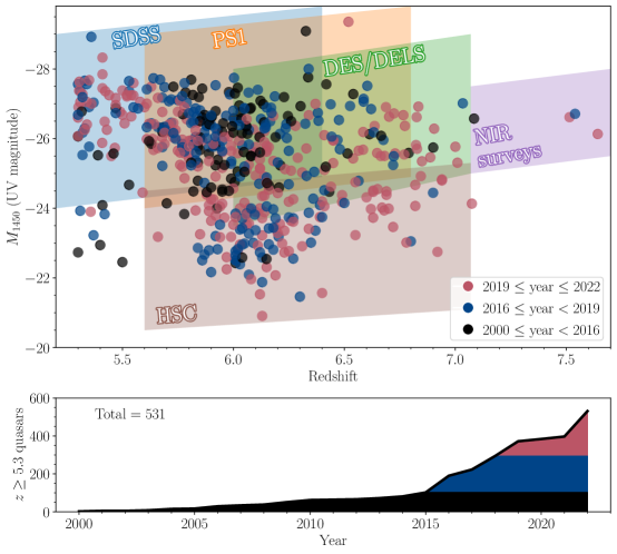
Figure 1: Distribution of all known $z\geq 5.3$ quasars in the absolute magnitude-redshift plane (top panel). The shaded areas are the parameter space probed by selected large quasar survey programs. The bottom panel shows the cumulative number of quasars known at $z\geq 5.3$ as a function of year of publication.

Fig. 1 presents the distribution of all published $z\geq 5.3$ quasars, as of Dec 2022, on the absolute magnitude-redshift plane, highlighting the major survey programs from which most of these quasars are selected. The progress illustrated by the bottom panel is a result of the availability of large scale optical and NIR sky surveys, improvements in selection and contaminant rejection, and efficient spectroscopic identification.

Quasar candidates are separated from other point sources in photometric surveys because of their distinct spectral energy distributions (SEDs). The intrinsic spectra of quasars (Fig 5) in the rest-frame UV and optical are characterized by a blue power-law continuum and a number of strong broad emission lines. At $z>3$, the strong IGM neutral hydrogen (HI) absorption from Lyman series lines and Lyman continuum redshifts into the observed optical wavelength. Thus high-redshift quasars are “dropout” objects with a strong Lyman break with the dropout bands correspond to the observed wavelength of the Lyman break. At longer wavelength, quasars have blue broad-band colors due to their power law continuum. The Lyman dropout selection method for quasars has been used since the discoveries of the first $z>4$ quasars (Warren et al., 1987). A more recent development is the inclusion of mid-IR (MIR) photometric surveys in the candidate selection (e.g. Wu et al., 2015). The long wavelength baseline from NIR to MIR, in particular using the WISE (Wright et al., 2010) data, allows more effective separation of high-redshift quasars and MLT dwarfs by colors.

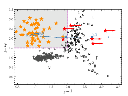
Figure 2: Example of y$-$J vs. J$-$W1 color-color diagram used for high-redshift quasar selections. The cyan line represents the average color-redshift relation for quasars at $z=6-7.3$ based on simulated quasar spectra. For a typical quasar spectrum, see Fig 5 Orange stars are known quasars at $6.5<z<7.0$; magenta line shows the selection criteria used by Wang et al. (2019) for this redshift range. Red stars are known quasars at $z>7.0$; black symbols are known MLT contaminants. Adapted from Wang et al. (2019).

Fig. 2 illustrates how to use the combination of optical and IR colors to select $z>6.5$ quasars. At $z\sim 6.5$, the strong Ly$\alpha$ emission line is in the $y$ band. At higher redshift, this band starts to be dominated by IGM absorption and quasars become “y-dropouts” with increasing red $y-J$ colors. Meanwhile, the $J-W1$ color is determined by the quasar power law continuum and has a near constant value, which is redder than most of the sub/stellar objects with spectral types earlier than L. The main contaminants for this redshift range are L and T dwarfs.

Inayoshi et al. (2020) presented a summary table of the photometric surveys used in the discoveries of $z>6$ quasars in the past fifteen years. Early surveys such as SDSS and PS1 (Chambers et al., 2016) used 2–4 meter class telescopes with relatively short exposure times, thus they are optimized to discover rare, luminous quasars in large sky areas. Selection of fainter quasars requires photometric observations on large aperture telescopes: the SHELLQs project (Matsuoka et al., 2022) is based on the Hyper Suprime-Cam (HSC) survey on the 8.2m Subaru Telescope (Aihara et al., 2018). As shown in Fig 2, at $z>7$, quasars begin to drop out in the $y$ band at the red limit of CCD detector sensitivities. The discovery of quasars at this redshift requires the combination of wide-field IR surveys that provide detection of the quasar rest-frame UV continuum, and deep optical surveys that sample the strong Lyman break. Following the first quasar discovery at $z>7$ using photometric data from the UKIDSS survey (Mortlock et al., 2011), there have been eight quasars published at $z>7$ (see Table 1). The current redshift frontier is represented by the three luminous quasars known at $z>7.5$, selected using a combination of NIR, optical, and MIR (WISE) surveys: J1342+0928 at $z=7.54$ (Bañados et al., 2018); J1007+2115 at $z=7.52$ (“Pōniuā’ena”, Yang et al., 2020b); and J0313-1806 at $z=7.64$ (Wang et al., 2021b).

2.2 Optimization of Photometric Selection of High-Redshift Quasars

The vast majority of high-redshift quasars have been discovered using color selection. The most commonly used method is to implement a series of “color cuts”: select objects that meet a set of criteria in the flux/flux-error space (usually referred to as the “color space”) as high-redshift quasar candidates. These cuts are often initially guided by a combination of photometry of existing high-redshift quasars and simulated colors based on synthetic quasar spectra, as well as observed and simulated data of the contaminant populations. These cuts are refined as surveys progress with larger training sets and better understanding of the contaminant populations. Fan (1999) presented an early example of color space simulation of different populations of objects with compact morphology (quasars, normal stars, white dwarfs and compact galaxies) in the SDSS photometric system. This simulation was used to formulate color selections for both the SDSS main spectroscopic survey (Richards et al., 2002) and selections of $z\sim 6$ quasars (Fan et al., 2001). Works such as Hewett et al. (2006), McGreer et al. (2013), Barnett et al. (2019), and Temple et al. (2021) expanded these simulations by including more realistic quasar population models and models of MLT and intermediate-redshift galaxies, extending to higher redshifts, and including NIR and MIR photometric bands.

High-redshift surveys based on SDSS (e.g., Jiang et al., 2016), PS1 (e.g., Bañados et al., 2016) as well as works using the DESI Legacy Survey (e.g., Wang et al., 2019) used color cuts as their primary selection method. The color cut method is simple to implement, and has high selection completeness even for objects that have unusual spectral features such as broad absorption lines (BALs), weak emission lines or those with modest reddening, because the color cuts are usually fairly loose and cover a large portion of color space, and the strong Lyman break is not strongly affected by the intrinsic quasar SEDs. On the other hand, because all candidates that satisfy the cuts are selected without considering the relative density distribution of the targeted (quasar) population and the contaminant populations (primary MLTs and compact galaxies), or how the candidate SEDs match the quasar template, color cut selection tends to have a higher contamination rate. For example, Wang et al. (2019) find a 30% spectroscopic success rate when searching for $z>6.5$ quasars. The contamination grows significantly worse for $z\sim 7.5$ (F. Wang, private communication).

A number of techniques have been applied to improve the efficiency of color selection. These improvements are especially important for quasars at the highest redshift ($z>6.5$), where quasars are increasingly rare compared to the contaminant populations, and at fainter fluxes for which increasing photometric errors results in more contaminants scatter into the selected area in color space. Mortlock et al. (2012) first introduced a selection algorithm based on Bayesian model comparison (BMC). In BMC, the posterior quasar probability for a given object with survey photometry $\bf{d}$ is given by :

$$P_{q}=p(q|\mathbf{d})=\frac{W_{q}(\mathbf{d})}{W_{q}(\mathbf{d})+W_{b}(\mathbf{d})+W_{g}(\mathbf{d})},$$ (1)

where q, b, and g represent quasar, brown dwarf (MLTs), and galaxy populations, respectively. The weights W for each population are calculated using a population model that describes its surface density distribution integrated over a Gaussian likelihood function based on model colors. BMC wss applied by Mortlock et al. (2011) to data from the UKIDSS survey to identify the first quasar at $z>7$. The SHELLQs survey (Matsuoka et al., 2022) used BMC to select faint quasars in the HSC survey with great success in achieving a high spectroscopic identification rate ($\sim 75\%$) even at the low-luminosity end at $z\sim 6$. Wagenveld et al. (2022) presented a similar probabilistic approach that also includes radio data in the selection.

Reed et al. (2017) applied a SED fitting method for high-redshift quasar selection. In this method, after the initial color cuts, reduced $\chi^{2}$ values are calculated for each candidate, matching the observed colors of the candidate observed SEDs to a series of model SEDs, including different MLT spectral types as well as early type galaxies at various redshifts. Objects with high reduced $\chi^{2}$ for the contaminant populations, and low values for the quasar SED models are selected as quasar candidates.

Barnett et al. (2021) presented a detailed comparison study of different selection techniques in searching for $z>6.5$ quasars using VIKING survey data. They show that BMC is highly complete in recovering previously known quasars in the survey area, and at the same time effectively rejects confirmed contaminants. Using simulations, they calculate the survey selection function – completeness as a function of quasar redshift and luminosity, and find that both BMC and the SED method represent a significant improvement in selection completeness and depth compared to simple color cuts.

Wenzl et al. (2021) used a random forest supervised machine learning method to select $z>5$ quasars from PS1 data with high efficiency. Nanni et al. (2022) proposed an alternative probabilistic approach, in which the density of the contaminant populations in color space is modeled as Gaussian mixtures based on observed photometric data and calculated using the extreme deconvolution technique, instead of using simulated population models.

High-redshift quasar selection can also be considered in the context of supervised machine learning. The training sets of existing objects are small, and in most case are subject to the bias of previously selected samples or extrapolations from low-redshift populations. The choice of high-redshift quasar selection algorithm in a given survey is a tradeoff between completeness and efficiency. Selections that rely on SED and contaminant population models run the risk of missing objects that are highly valuable but have unusual properties. An example is the discovery of J0100+2802, the most luminous unlensed quasar currently known at $z>5$ (Wu et al., 2015). The object was assigned as low priority in the original SDSS survey due to its relatively red color and bright apparently magnitude, indicating high probability of it being a brown dwarf. It is not surprising that record-breaking discovery is made often – but not always (e.g., Mortlock et al., 2011) – using the less restrictive color-cut method, and probabilistic methods are more effective once a large training set has been established.

If high-redshift quasar candidates could be part of the overall target selection in a large automated spectroscopic survey program, then the color selection could be relaxed to be more complete and less sensitive to templates or model assumptions, because high-redshift quasar candidates are rare and are thus only a small fraction of the total targets. The SDSS main quasar survey (Richards et al., 2002) targeted quasars up to $z\sim 5.4$. The Dark Energy Spectroscopic Instrument (DESI, Abareshi et al., 2022) is using spectrographs with 5000 fibers on the 4-m Mayall Telescope at Kitt Peak to conduct a 5-year spectroscopic survey of $\sim 40$ million galaxies, quasars and stars. DESI is expected to more than double the number of quasars known at $z>5$ when completed. A similar survey is being planned for the 4MOST project (Merloni, 2019).

Other established quasar selection methods include variability, astrometry (i.e., lack of proper motion; Lang et al., 2009), detections in X-ray and radio wavelengths, MIR colors, as well as wide-field slitless spectroscopy. Except for the last method (e.g., Schneider et al., 1989, 1999), most selection methods are not sensitive to the quasar redshifts. Therefore, some color cuts are usually used to identify high-redshift quasar candidates. McGreer et al. (2006) and Zeimann et al. (2011) report the first discoveries of radio-loud $z>6$ quasars by matching radio surveys such as FIRST with optical photometric surveys. X-ray observations provide fundamental probes of AGN evolution across cosmic time. New wide-field X-ray surveys such as e-ROSITA (Wolf et al., 2021) will enable selections of luminous X-ray quasars at the highest redshifts. We will discuss the X-ray and radio properties of high-redshift quasars in Sec 3.2.

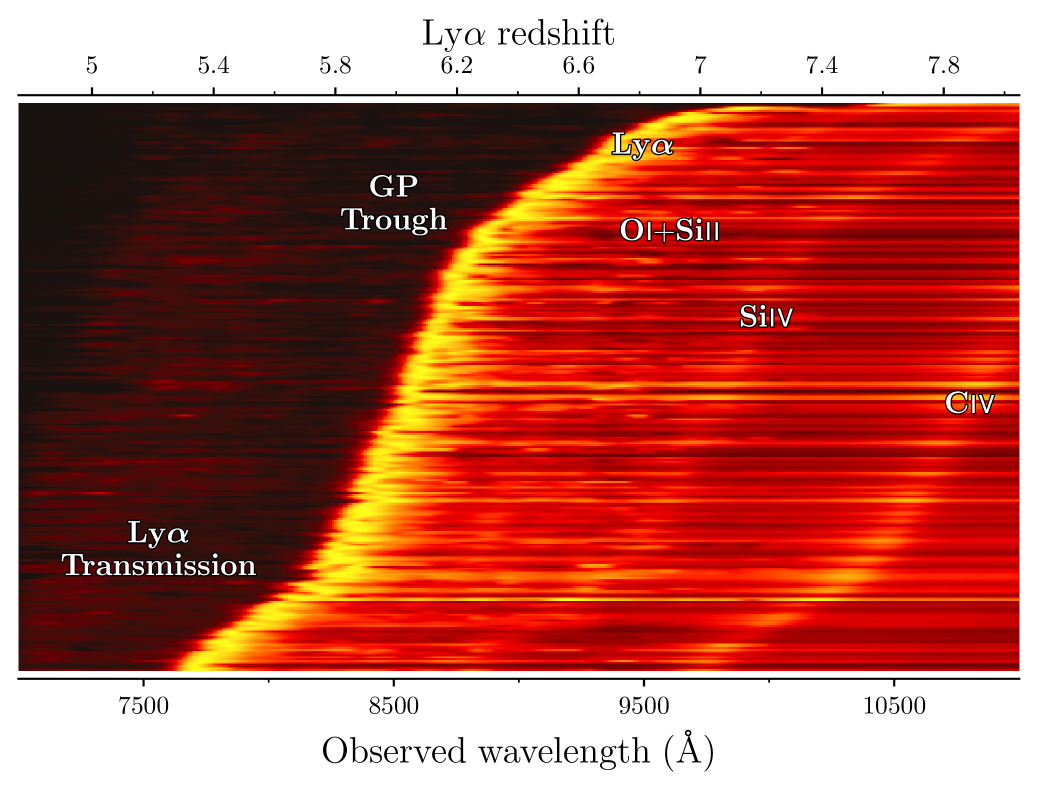
Figure 3: Two-dimensional image representation of 527/531 of all published spectra of $z\geq 5.3$ quasars. Traces of major emission lines are labeled. On the blue side of Ly$\alpha$ line, there are clear signatures of the Ly$\alpha$ transmission at $z<6$, while at higher redshift, the spectra are dominated by long Gunn-Peterson absorption troughs.

2.3 A Database of $z>5.3$ Quasars

At the time of this review, there are 531 $z\geq 5.3$ quasars in the published literature. We present their spectra in Fig 3. The locations of the $z\geq 5.3$ quasars on the redshift-luminosity plane is shown in Fig 1. We include a database with their basic properties in the Supplementary Material associated with this review (follow the Supplemental Material link from the Annual Reviews home page at http://www.annualreviews.org). To be included in this database, we require the object to : (1) have a spectroscopically confirmed redshift $z\geq 5.3$; we do not include objects with only photometric redshifts; (2) have at least one broad emission line (FWHM $>2000$ km s^-1) in the rest-frame UV; we do not include narrow-line (Type-2) quasars or obscured AGN at high redshift. In addition to the quasar name, coordinates, redshift and references, the database also include measurements of the quasar’s continuum luminosity at the rest-frame 1450 Å and 3000 Å, properties of the Mg ii emission line, and BH mass derived from Mg ii measurements quoted in the literature, estimated using Equation 4. We only consider Mg ii measurements for quasars at $z>5.9$, as Mg ii lines are usually in regions highly affected by telluric absorption in the NIR at lower redshift.

Table 1: Quasars at $z>7$

Quasar	$z$	$M_{1450}$	$M_{\rm BH}$	Disc. ref.	$M_{\rm BH}$ ref.
		$\mathrm{mag}$	$10^{8}\,M_{\odot}$
J031343.84–180636.40	$7.6423$	$-26.13$	$16.1$	Wang et al. (2021b)	Yang et al. (2021)
J134208.11+092838.61	$7.54$	$-26.71$	$8.1$	Bañados et al. (2018)	Yang et al. (2021)
J100758.27+211529.21	$7.5149$	$-26.62$	$14.3$	Yang et al. (2020b)	Yang et al. (2021)
J112001.48+064124.30	$7.0848$	$-26.58$	$13.5$	Mortlock et al. (2011)	Yang et al. (2021)
J124353.93+010038.50	$7.0749$	$-24.13$	$3.6$	Matsuoka et al. (2019b)	Matsuoka et al. (2019b)
J003836.10–152723.60	$7.034$	$-27.01$	$13.6$	Wang et al. (2018)	Yang et al. (2021)
J235646.33+001747.30	$7.01$	$-25.31$	–	Matsuoka et al. (2019a)	–
J025216.64–050331.80	$7.0006$	$-25.77$	$12.8$	Yang et al. (2019b)	Yang et al. (2021)

The high-redshift quasar database includes 275 objects at $z>6$ and 8 at $z>7$. At the time of writing, there are 113 $z>5.9$ quasars with robust Mg ii-based black hole mass estimates. We list the properties of quasars currently known at $z>7$ in Table 1. This database expands the compilation in the Supplementary Material of Inayoshi et al. (2020). The quasar luminosities lie between $M_{1450}=-20.9$ and $-29.4$; the median luminosity of these objects is $M_{1450}=-25.8$. The brightest object is J0439+1634, a gravitationally lensed quasar at $z=6.5$ (Fan et al., 2019b). Fig 3 shows a two-dimensional image representation of all spectra of the quasars in the database. In this image, each row is the one-dimensional spectrum of a quasar, ordered in ascending redshift. The flux level of each column is normalized by its peak Ly$\alpha$ flux. The image shows how the quasar Ly$\alpha$ emission line move to near-IR wavelengths as the redshift increases from $z\sim 5$ to $>7$. On the blue side of the Ly$\alpha$ emission, the spectra show the extent of the highly ionized quasar proximity zone (Sec 6.3.1), where the flux does not immediately drop to zero. Further blueward, the spectrum is dominated by strong Gunn-Peterson absorption. Complete Gunn-Peterson absorption troughs can be seen at $z>6$. At lower redshift, the presence of transmission spikes indicates that the IGM is, on average, highly ionized (Sec 6). On the red side of Ly$\alpha$ emission, broad emission lines such as OI+SiII$\lambda 1306$, SiIV+OIV]$\lambda 1402$ and CIV$\lambda 1549$ are visible.

2.4 Future Quasar Surveys

New surveys are on the horizon to further expand the quasar redshift frontier. The Legacy Survey of Space and Time (LSST) by the Vera C. Rubin Observatory will cover the southern sky at optical wavelengths to unprecedented depths. LSST will reach 5$\sigma$ co-added depths in the $z$ and $y$ bands at $25-26$ mag level in 5-10 years (Ivezić et al., 2019), allowing selections of several thousand quasars and AGN at $z\sim 6-7.5$ using both color and variablity selection methods, while providing deep photometry in the dropout bands for selection of $z>7$ quasars. ESA’s Euclid mission will provide deep near-IR photometry not possible with ground-based observations. It will cover 15,000 deg² of the sky to a 5$\sigma$ depth of 24 mag in Y, J and H bands (Scaramella et al., 2022), enabling selection of quasar candidates up to $z\sim 10$. Barnett et al. (2019) predicted that Euclid + LSST will allow discoveries of $\sim 25$ quasars at $z>7.5$, including $\sim 8$ beyond $z>8$, although the exact yields strongly depend on the assumed evolution of quasar luminosity function. Further in the future is NASA’s Nancy Grace Roman Space Telescope, which will cover a smaller area in its High Latitude Survey but reaching about two magnitude deeper.

Fan et al. (2019a) show that by extrapolating the current measurement of the quasar luminosity function, there will be only one “SDSS”-like quasar ($M_{1450}<-26$, powered by billion-M_⊙ SMBH) over the entire observable universe at $z>9$. The combination of LSST, Euclid and Roman will allow the discovery of the earliest luminous quasars in the Universe. However, in addition to the challenges of their selection (Barnett et al., 2019, Nanni et al., 2022), their spectroscopic identification will require IR spectrographs more powerful than those with the current ground-based telescopes: 30m-class extremely large telescopes and JWST will be the primary tools for their confirmation and follow-up observations.

3 AN EVOLVING QUASAR POPULATION

In this section, we first review the evolution of the quasar luminosity function (QLF) at high redshift, which directly constrains the growth history of early SMBHs (Sec 3.1). The number density of quasars is found to decline rapidly towards high redshift, in sharp constrast to the lack of strong evolution in the SEDs of quasars (Sec 3.2), from X-ray to radio, and in particular in the rest-frame UV to NIR, at which the quasar SED peaks, although a number of sub-types of quasars appear to be more common at $z>5-6$.

3.1 Evolution of Quasar Luminosity Function

Soon after the initial discovery of quasars, Schmidt (1968) found that their density rises sharply with redshift up to $z\gtrsim 2$. Wide-field surveys such as 2dF (Boyle et al., 2000) and SDSS (Richards et al., 2006b) established that the density of luminous quasars peaks at $z\sim 2-3$. Osmer (1982) presented the first evidence that quasar density at $z>3.5$ appears to be declining. Schmidt et al. (1995) characterized this decline as an exponential function with redshift:

$$\rho(z)\propto 10^{kz},$$ (2)

where $k$ is measured to be $\sim-0.5$ at $z\sim 3-5$. The shape of the QLF is usually described as a double, or broken, power law:

$$\Phi(M_{\mathrm{1450}},z)=\frac{\Phi^{\ast}(z)}{10^{0.4(\alpha+1)(M_{\mathrm{1450}}-M^{\ast}_{\mathrm{1450}})}+10^{0.4(\beta+1)(M_{\mathrm{1450}}-M^{\ast}_{\mathrm{1450}})}}$$ (3)

where $M_{\mathrm{1450}}$ is the absolute magnitude of the quasar continuum at rest-frame 1450 Å, $\alpha$ and $\beta$ are the faint-end and bright-end slopes, respectively, $M^{\ast}_{\mathrm{1450}}$ is the characteristic absolute magnitude or break magnitude measured at 1450 Å, and $\Phi^{\ast}$ is the normalization of the LF which has an exponential decline described in Eq. 2.

Early high-redshift surveys such as the SDSS were only sensitive to the most luminous quasars. Based on a sample of nine SDSS quasars at $z>5.7$, Fan et al. (2004) found that at $z\sim 6$, the co-moving spatial density of quasars with $M_{1450}<-26.7$ is $6\times 10^{-10}\rm Mpc^{-3}$, consistent with extrapolation from lower redshift trends. Jiang et al. (2009) extended the SDSS quasar survey to the “stripe 82” region, reaching two magnitudes deeper than the SDSS main survey. They found a bright end slope $\beta$ between –2.6 and –3.1. Willott et al. (2010) combined the faint quasars discovered in the Canada-France High-z Quasar Survey (CFHQS) with the brighter SDSS quasars, and presented the first measurement of QLF at $z\sim 6$ using a sample of 40 quasars. They found a bright end slope $\beta=-2.81$ and a break magnitude $M^{*}_{1450}=-25.1$; the faint end slope was still poorly constrained at this redshift. Jiang et al. (2016) presented the final results of the $z\sim 6$ quasar survey in the SDSS footprint. Using this sample of 52 quasar at $5.7<z<6.4$, they found a bright end slope of $\beta=-2.8\pm 0.2$. In addition, they found a density evolution with the exponential evolution parameter $k=-0.72\pm 0.11$, a significantly steeper slope than the value at $z\sim 3-5$, suggesting an accelerated evolution of luminous quasars between $z\sim 5$ and 6.

The SHELLQs project (Matsuoka et al., 2016) extended the $z\sim 6$ quasar sample to significantly lower luminosity. Matsuoka et al. (2018) presented measurements of the QLF down to $M_{1450}\sim-22$, which is well fit with a double power law that has a faint-end slope $\alpha=-1.23^{+0.44}_{-0.34}$, a bright-end slope $\beta=-2.73^{+0.23}_{-0.31}$, and a break magnitude $M^{*}_{1450}=-24.90^{+0.75}_{-0.90}$. Their measured QLF showed a strong break and a significant flattening at the faint end at $z\sim 6$. Schindler et al. (2022) used the combination of the bright PS1 quasar sample that includes 125 quasars at $z\sim 5.7-6.2$ with the fainter quasars from SHELLQs for a new QLF measurement at $z\sim 6$. They found a steeper bright-end slope of $\beta=-3.84^{+0.63}_{-1.21}$, as well as a steeper faint-end slope of $\alpha=-1.70^{+0.29}_{-0.19}$, with a bright break magnitude of $M^{*}_{1450}=-26.38^{+0.79}_{-0.60}$. Their study yields a constant redshift evolution of $k\sim-0.7$ over a wide redshift range of $z=4-7$.

Measurement of the QLF becomes increasingly difficult at higher redshift due to the rapid decline in spatial density of quasars. Wang et al. (2019) conducted the first measurement of the QLF at redshift approaching seven based on a sample of 17 quasars at $6.45<z<7.05$ (see also Venemans et al., 2013). They found a quasar spatial comoving density of $\rho(M_{1450}<-26)=0.39\pm 0.11\rm Gpc^{-3}$ at $z\sim 6.7$, and an exponential density evolution parameter $k=-0.78\pm 0.18$. The density of luminous quasars declines by a factor of $\sim 6$ per unit redshift. The e-folding time of quasar density evolution and that of black hole accretion (Sec 4) become comparable, underlying the strong constraints quasar evolution could place on the SMBH accretion mode.

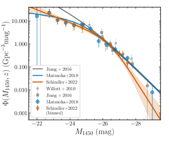
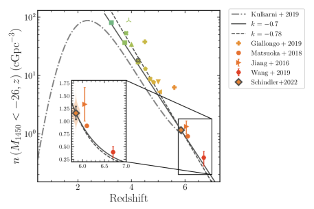
Figure 4: Quasar luminosity function measurements at high-redshift. (left): the QLF at $z\sim 6$ from SDSS, CFHTQS, SHELLQs, and PS1 surveys and best-fit double power law results. (right) The density of luminous ($M_{1450}<-26$) quasars as a function of redshift (for measurements at $z<5.3$, see references in Schindler et al. 2022). Figures adapted from Schindler et al. (2022).

Fig 4 (right panel) illustrates the overall density evolution of luminous ($M_{1450}<-26$) quasars with measurements from various surveys at $z=3-7$. While a strong exponential decline in the comoving spatial density of luminous quasars has been well established, there are still significant uncertainties in the evolution of the shape of the QLF (Fig 4, left panel). As discussed in Schindler et al. (2022), the bright-end slope determination is strongly influenced by small number statistics. At the faint end, selection incompleteness could be a significant factor when a completeness correction of $\gtrsim 2$ is often needed.

There have been a number of ambitious efforts to combine QLF measurements across the electromagnetic spectrum and different cosmic epochs to obtain a complete picture of quasar/AGN evolution from reionization to the current epoch. Hopkins et al. (2007) presented the bolometric QLF up to $z\sim 6$. They explicitly modeled the X-ray column density distribution and SED shape variation of quasars to allow determinations of bolometric luminosities of high-redshift populations. Kulkarni et al. (2019) constructed a sample of more than 80,000 color-selected quasars and AGN with a homogeneous treatment of survey selection effects, and derived the AGN UV luminosity function from $z=0$ to 7.5. Their measurement suggested a continued steeping of the faint end slope $\beta$ and a brightening of the break magnitude. Shen et al. (2020) updated the early Hopkins et al. work. They found bolometric QLF evolution consistent with those based on UV-selected samples alone, and concluded that the faint-end slope measurement is still uncertain at high-redshift.

For the purpose of comparison with theoretical models or making predictions of future surveys, we suggest using the combined QLF measurements presented in Kulkarni et al. (2019) or Shen et al. (2020) for $z\lesssim 6$, where the QLF is well measured over a wide range of luminosity. At $z\gtrsim 6$, the uncertainty is still large for both the QLF shape and its redshift evolution; Schindler et al. (2022) presented the most up-to-date measurements.

A key limitation of current high-redshift quasar surveys is that the quasar selection methods assume a blue power-law continuum in the rest-frame UV. It is possible that current surveys are missing significant number of red or reddened quasars. Kato et al. (2020) reported the discovery of two dust-reddened quasars at $z>5.6$ in the SHELLQs survey based on their mid-IR WISE detection. Endsley et al. (2022) discovered an obscured radio-loud AGN at $z=6.85$ in the 1.5 deg² COSMOS field with bolometric luminosity comparable to that of luminous SDSS $z\sim 6$ quasars. Ni et al. (2020) studied the obscuration of high redshift quasars using the BLUETIDES simulation, and predicted that the dust-extincted UV LF is about 1.5 dex lower than the intrinsic LF, and the vast majority of $z\sim 7$ AGNs have been missed by UV-based surveys due to dust extinction. This would imply a much higher bolometric luminosity density of early quasars, and would have a profound impact on the growth of SMBHs and early galaxy evolution overall. A reliable determination of the obscured fraction of quasars at $z\gtrsim 5$ needs a combination of wide-field deep X-ray survey and effective spectroscopic identification of faint, obscured sources with either JWST or NOEMA/ALMA.

3.2 (A Lack of) Evolution of the Quasar Spectral Energy Distributions

High-redshift galaxies have intrinsic blue SEDs that are dominated by young stellar populations. Metallicity, or chemical abundance, in their ISM has also been shown to be lower than in low-redshift galaxies (Stark, 2016). However, the overall SEDs and the chemical abundance in quasar broad line regions (BLRs) do not evolve significantly with redshift, although quasar density decreases drastically at high-redshift. This apparent lack of spectral evolution in the UV properties of quasars were noticed as soon as the first $z\sim 6$ quasars were discovered (e.g., Barth et al. 2003, Fan et al. 2004, Iwamuro et al. 2004, Jiang et al. 2007). Shen et al. (2019) conducted an optical/NIR spectroscopic survey of 50 quasars at $z>5.7$. Their observations covered the wavelength range from the Ly$\alpha$ to Mg ii emission lines. Yang et al. (2021) presented a spectroscopic survey of 34 quasars at $6.3<z<7.6$, covering a similar wavelength range. Both papers presented composite rest-frame UV spectra of their high-redshift samples. Fig 5 compares the quasar composite spectra at $z\sim 6-7$ with the standard low-redshift SDSS quasar composite from Vanden Berk et al. (2001). The average continuum slope and emission line strength/width do not evolve significantly with redshift, with the exception of a weaker and blueshifted C iv emission line (see discussion in Sec 5.4).

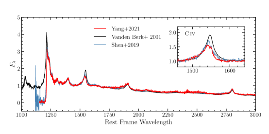
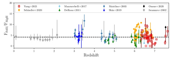
Figure 5: Upper panel: Quasar composite spectrum (red solid line) from Yang et al. (2021) compared with the low-redshift ($z\lesssim 3$) composite from Vanden Berk et al. (2001); black line) and the $z\sim 6$ quasar composite from Shen et al. (2019); blue line). The average intrinsic spectrum of quasars does not exhibit significant redshift evolution. Lower panel: the evolution of the Fe/Mg emission line radio in quasars as a function of redshift. The quasar BLR is highly enriched even at the highest redshift. Adapted from Yang et al. (2021).

Broad emission line ratios in quasars have been used to constrain metallicities in the quasar BLR. Jiang et al. (2007) and De Rosa et al. (2014) studied emission line ratios in a series of UV lines, and found no evidence of evolution from lower redshift samples, with the gas metallicity a few times solar based on photoionization modeling. This is confirmed by studies using high S/N spectroscopy from the XQR30 survey (https://xqr30.inaf.it/) of quasars at $z=5.8-7.5$ (Lai et al., 2022). The line ratio of Fe ii/Mg ii is of particular interest, because of the different enrichment histories of these two lines – Mg is an $\alpha$-element predominately produced by core-collapse supernovae, while Fe is mainly from Type-1a supernovae with an evolutionary lifetime delay of a few hundred million years to 1 Gyr. The evolution of the Fe/Mg ratio in quasars has been studied extensively (e.g., Barth et al., 2003, Iwamuro et al., 2004, De Rosa et al., 2014, Mazzucchelli et al., 2017b, Shen et al., 2019, Yang et al., 2021). Schindler et al. (2020) carried out detailed modeling of Fe ii and Mg ii lines using a large sample of quasar spectra from VLT/Xshooter, and compared their measurements with those in the literature. There is no evidence of evolution in the Fe/Mg ratio up to the highest redshift, although scatter is large at any given redshift (Fig 5). The lack of spectral evolution in quasar rest-frame UV spectra, especially in the emission line properties, indicates that quasar BLRs are chemically enriched very rapidly, within the first few hundred million years after the initial star formation in the host galaxy. This is not surprising, as we will review in Sec 5: quasar host galaxies are sites of the most intense star formation in the early universe.

However, there are a few noticeable evolutionary trends in quasars at cosmic dawn that could be related to the early phase of quasar growth. In Sec 5.4, we discuss an increasing fraction of quasars with strongly blue-shifted high ionization UV emission lines and with strong BAL features as evidence for early quasar feedback. In Sec 6.3.1, we present the discovery of $z\sim 6$ quasars with IGM absorption features indicative of very young ages.

A subset of high-redshift SDSS quasars have much weaker UV emission lines, in particular Ly$\alpha$ and C iv. Diamond-Stanic et al. (2009) identified them as $>3\sigma$ outliers in the quasar emission line strength distributions. They represent $\sim 1\%$ of quasar population at $z<4$, after correction for selection incompleteness (Diamond-Stanic et al., 2009). Bañados et al. (2016) showed that this fraction increases to $\sim 14\%$ among $z>5.6$ PS1 quasars based on Ly$\alpha$ measurements. Shen et al. (2019) found a similar fraction using C iv measurements. It remains unclear whether weak line quasars are related to the young age or high accretion rate in the high-redshift quasar population (Plotkin et al., 2015)..

X-ray emission originates from the accretion disk and surrounding hot corona close to the central SMBH, and provides crucial information about black hole accretion and AGN feedback (Fabian, 2012). Brandt et al. (2001) detected the first $z\sim 6$ quasar in X-rays using the XMM/Newton telescope. More than 30 quasar at $z\gtrsim 6$ have now been detected in X-rays, using either the Chandra or XMM-Newton telescopes. Nanni et al. (2017) analyzed 29 quasars at $z>5.5$ with X-ray detections. They found a mean X-ray power-law photon index of $\Gamma\sim 1.9$, similar to that at low redshift. The optical-X-ray spectral slopes of the high-redshift also follow the relation established at low redshift. Vito et al. (2019a) carried out a similar analysis, and found a slightly steeper X-ray power-law index, consistent with a generally higher Eddington ratio among SMBHs in these quasars at $z>6$. Wang et al. (2021a) extended the X-ray analysis to quasars at $z\sim 7$ (see also Pons et al., 2020). They also found a steepening of X-ray spectra with $\Gamma\sim 2.3$. The optical-X-ray power-law slope, $\alpha_{OX}$, traces the relative importance of the accretion disk and corono emission in quasars and AGN. At low redshift, there is a tight correlation between $\alpha_{OX}$ and the quasar UV luminosity (e.g. Just et al., 2007). There is no evolution in this correlation up to $z\sim 7$ (e.g. Wang et al., 2021a). The X-ray observations show a consistent picture that the inner accretion-disk and hot-corona structure in quasars was established at the highest redshift with minimal evolution in their properties across cosmic time.

At rest-frame NIR and MIR wavelengths, the radiation from quasars is dominated by reprocessed emission from the hot dust component beyond the accretion disk structure (see review by Lyu & Rieke, 2022). At the highest redshift, dust observations (at rest-frame $>1.5\,\mu$m) have been largely limited to photometric observations of bright sources using the Spitzer (e.g., Jiang et al., 2006) and Herschel (Leipski et al., 2014) Telescopes, although this will change with the launch of JWST. These observations also showed a lack of evolution: the average IR-SEDs of quasars at $z\sim 5-6$ are consistent with low-redshift templates and the hot dust structure is already in place by $z\sim 6$. Jiang et al. (2010) reported the detection of two quasars at $z\sim 6$ with weak hot dust emissions using Spitzer. Later studies suggested that these dust-deficient quasars are not unique to $z>6$, and examples with similar SEDs are found even in the low-redshift PG sample (e.g. Lyu et al., 2017).

Quasars were initially discovered as point-like sources emitting strong radio emissions (Schmidt, 1963). However, the fraction of quasars that exhibit strong jet-powered radio emission (radio-loud quasars) is around 10% with no significant dependence on redshift, at least up to $z\sim 6$ (Bañados et al., 2015, Liu et al., 2021, Gloudemans et al., 2021). The highest redshift radio-loud quasar known is at $z=6.82$ (Bañados et al., 2021), and the highest redshift blazar is at $z=6.10$ (Belladitta et al., 2020). It is still debated whether the seemingly constant radio-loud fraction is due to two intrinsically different populations of quasars or is a consequence of the duty cycle of jet emission during the life of a quasar. If the latter were the case, one should expect an increase in the radio-loud fraction at the highest redshifts (where the available time for a quasar shortens), something we have not yet witnessed and depends on the lifetime of the radio-loud phase.

The lack of evolution in the radio-loud fraction discussed above concerns the compact core radio emission. However, there is an important evolution with redshift if we focus on the extended radio emission: the lack of giant ($\sim$100s kpc) radio lobes at $z>4$, which are common at lower redshifts (Fabian et al., 2014). Indeed, the most extended radio jet known at $z\sim 6$ is $<2\,$kpc (Momjian et al., 2018). A plausible physical explanation is that at $z>4$, the CMB energy density [$\propto(1+z)^{4}$] exceeds the magnetic energy density in radio lobes. In that case, inverse Compton (IC) scattering losses will make any large lobes at high redshift radio weak and X-ray bright (Ghisellini et al., 2014). The IC/CMB effect has been challenging to probe with current X-ray telescopes. Recent deep Chandra X-ray observations of the two $z\sim 6$ quasars with the most extended radio jets resulted in tentative evidence of larger X-ray jets (Connor et al., 2021, Ighina et al., 2022). Obtaining this marginal evidence was expensive, even for our most powerful X-ray telescopes observing the best existing targets to test this effect. To robustly measure the IC/CMB effect in a sample of radio-loud quasars, we will likely need to wait for the next generation of X-ray telescopes.

The discussions in this subsection present a picture that on average, the intrinsic SED of quasars at the highest redshift, with emission from the accretion disk (X-ray, UV/optical), broad emission line regions, hot dust, and radio jets, show little evolution from their low-redshift counterparts. The AGN structure is already in place and fully formed up to the highest redshift we have observed to date.

JWST will enable detailed studies of the physical properties of high-redshift quasars in the rest-frame optical and IR wavelengths which are not possible from the ground. It will be especially interesting to see if the dust component of the quasar population shows any evolution, since dust production mechanism (e.g. Maiolino et al., 2004) and the ISM conditions in the host galaxies are likely different in early epochs. X-ray observations with Chandra and XMM of even the most luminous quasars at cosmic dawn can only yield a small number of photons. Future X-ray missions (e.g. Martocchia et al., 2017) could allow allow high S/N spectroscopic observations of early quasars to characterize their accretion properties (including BH spin) and X-ray obscuration.

4 GROWTH OF SUPERMASSIVE BLACK HOLES IN THE FIRST BILLION YEARS

SMBHs are thought to be ubiquitous in the centers of massive galaxies, but their formation mechanism is still an outstanding question in astrophysics. Since the discovery of quasars at $z\gtrsim 6$ (Fan et al., 2001), the formation and growth of SMBHs have become even more intriguing and challenging to explain. In this section we will first review the current methods used to measure the BH masses at high redshift (Section 4.1), then give an overview of the properties of the observed population (Section 4.2), and the implications for early BH seeds and growth (Section 4.3). Finally, we will briefly describe additional methods that in the near future can be used to improve current BH mass estimates at high redshift (Section 4.4).

4.1 Black Hole Mass Measurements in High-redshift quasars

The spectra of $z\gtrsim 6$ quasars show the typical signatures of broad (FWHM of thousands ${\rm\,km\,s^{-1}}$) emission lines that are superimposed on the power-law continuum emission of the quasar’s accretion disk. These broad lines are thought to emerge from a region very close to the accreting BH (so-called the “broad-line region”) and thus provide a unique tool to constrain the properties of the central BH. The size of the broad-line region scales with the quasar luminosity, and the width of the lines is a measure of the potential depth (Peterson et al., 2004). Thus, a single-epoch spectrum gives enough information to estimate the mass of the central accreting BH (Vestergaard & Osmer, 2009).

One of the most reliable estimators of BH mass and Eddington ratio is the H$\beta$ line (e.g., Park et al. 2012). At $z>6$, H$\beta$ is shifted to the MIR and is thus not accessible from the ground. As an alternative, the C iv $\lambda$1549 and Mg ii $\lambda$2800 lines have been extensively used to measure BH masses of quasars at these redshifts (e.g., De Rosa et al. 2014, Farina et al. 2022). Estimates based on the high ionization C iv line are uncertain, as this line shows large velocity offsets, implying significant non-virialized motions (Mejía-Restrepo et al. 2018, Park et al. 2017). Moreover, there is mounting evidence that large C iv blueshifts ($>2000\,{\rm\,km\,s^{-1}}$) are more common at $z>6$ than at lower redshifts (e.g., Meyer et al., 2019, Schindler et al., 2020, see also Section 5.4). Therefore, in this review, we only focus on results based on Mg ii measurements, which are thought to be the most reliable until H$\beta$-derived masses are possible (Bahk et al. 2019; see Section 4.4).

One of the most widely used relations for BH mass estimation in high-redshift quasars is:

$$M\mathrm{{}_{BH}}=10^{6.86}\,\left[\frac{\mathrm{FWHM(\text{Mg\,{ii}})}}{1000\,\mathrm{km\,s^{-1}}}\right]^{2}\,\left[\frac{L3000}{10^{44}\,\mathrm{erg\,s^{-1}}}\right]^{0.5}\,M_{\odot},$$ (4)

where FWHM(Mg ii) is the Full Width at Half Maximum of the Mg ii line, and L3000 is the luminosity at 3000 Å. Vestergaard & Osmer (2009) presented the scaling relation from Equation 4. The intrinsic scatter in the relation is 0.55 dex, which dominates the uncertainty for individual measurements.

The theoretical maximum luminosity that a source can achieve when the gravitational and radiation forces are in equilibrium is called the Eddington luminosity (Eddington, 1926). The Eddington luminosity for pure ionized hydrogen in spherical symmetry is defined as

$$L_{\rm Edd} = \dfrac{4\pi cGm_{p}M_{\rm BH}}{\sigma_{T}}$$

$$= 1.26\times 10^{38}\,{\rm\,erg\,s^{-1}}{}\left(\dfrac{M_{\rm BH}}{M_{\odot}}\right)$$

where $c$ is the speed of light, $G$ is the gravitational constant, $m_{p}$ is the mass of a proton, and $\sigma_{T}$ is the Thomson scattering cross-section. The ratio between the bolometric and Eddington luminosities (referred to as Eddington ratio; $\lambda_{\rm Edd}=L_{\rm Bol}/L_{\rm Edd}$) is useful to assess the quasar population’s accretion properties. While several bolometric corrections are published in the literature (e.g., Runnoe et al. 2012, Trakhtenbrot & Netzer 2012, Duras et al. 2020), in this review (e.g., in Fig. 6), we adopt the bolometric correction first presented by Richards et al. (2006a) and used in several studies of high-redshift quasars (e.g., Shen et al., 2011, Yang et al., 2021, Farina et al., 2022):

$$L_{\textrm{bol}}=5.15\times L3000,$$ (6)

Farina et al. (2022) argued that bolometric luminosities estimated using equation 6 are on average in between the ones calculated using the bolometric corrections from Runnoe et al. (2012) and Trakhtenbrot & Netzer (2012). In the high-redshift quasar database presented in Supplementary Material we report $L3000$ so the readers can apply their preferred bolometric correction.

4.2 Current Demographics

At redshifts $6.0\lesssim z\lesssim 7.6$, the Mg ii line falls in the NIR K band. The vast majority of the Mg ii-based BH masses come from NIR spectra taken with powerful ground-based telescopes such as Gemini, VLT, Magellan, and Keck (Shen et al., 2019, Onoue et al., 2019, Yang et al., 2021, Farina et al., 2022). At the time of writing, there are 113 quasars at $z>5.9$ with reliable Mg ii-based black hole mass estimates. Currently, there is a strong bias towards luminous ($\gtrsim 10^{46}\,$erg s^-1) quasars, but obtaining reliable measurements for fainter sources is challenging with current facilities (see Onoue et al. 2019). We will need JWST and ELTs to enlarge the sample towards the faint end significantly. Fig. 6 shows the bolometric luminosity and BH mass distribution for all quasars with Mg ii-based masses at $z>5.9$. The median BH mass is $1.3\times 10^{9}\,M_{\odot}$, while the least and most massive quasars are J0859+0022 at $z=6.39$ ($\sim$$4\times 10^{7}\,M_{\odot}$; Onoue et al. 2019) and J0100+2802 at $z=6.33$ ($\sim$$10^{10}\,M_{\odot}$; Wu et al. 2015), respectively.

The first samples of NIR spectroscopic observations of $\gtrsim 6$ quasars showed that they accrete close to the Eddington limit, i.e., $\lambda_{\rm Edd}\approx 1$ (e.g., Willott et al., 2003, Kurk et al., 2007, De Rosa et al., 2011). Extending the measurements to larger samples (Shen et al., 2019) or probing to fainter luminosities (Onoue et al., 2019) revealed a significant number of quasars accreting at sub-Eddington rates. The recent works by Yang et al. (2021) and Farina et al. (2022) analyzed some of the largest samples of NIR spectra of $z\gtrsim 6$ quasars. Yang et al. (2021) studied 37 quasars at $z>6.3$ and found that these quasars have significantly higher Eddington ratios (mean of 1.08 and median 0.85) than a luminosity-matched quasar sample at low redshift. Farina et al. (2022) studied the NIR spectra of 135 $z\gtrsim 5.7$ quasars (including BH properties derived from Mg ii and C iv), finding that at $z\sim 6$ the Eddington ratio distributions are consistent with a luminosity-matched low-redshift sample independent of the luminosity, while there is evidence for a mild increase in the median Eddington ratios for $z\gtrsim 6.5$ (in agreement with Yang et al. 2021).

In our current compilation (Fig. 6), the Eddington ratio ranges from $0.08$ to $2.70$, with a median of 0.79 and a mean of 0.92. Forty quasars exceed the nominal Eddington limit, and eight have $\lambda_{\rm Edd}>2$. These values must be considered with caution as there is a substantial scatter in the BH mass estimations (see Section 4.1).

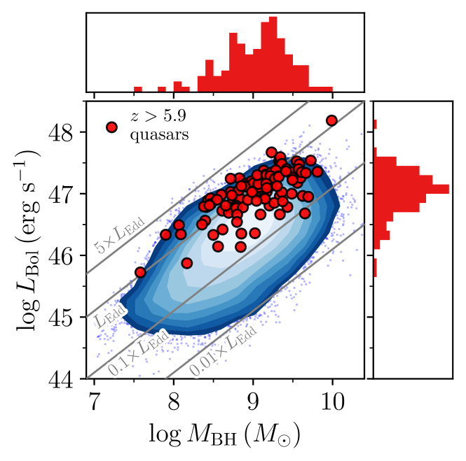
Figure 6: Bolometric luminosity vs. BH mass. The blue contours and points show the distribution for low-redshift SDSS quasars while the red circles are measurements for $z>5.9$ quasars. Solid gray lines show the location of constant accretion rate at 0.01, 0.1, 1, and 5 times the Eddington luminosity. All BH masses are from Mg ii measurements using equation 4 and the bolometric luminosities are derived using Equation 6.

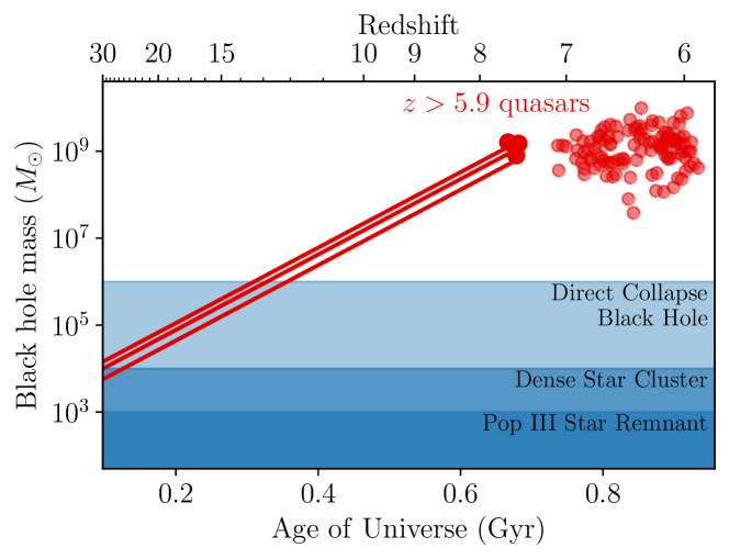
Figure 7: BH growth history: BH mass vs. age of the Universe (redshift at the top). The red circles mark our compilation of robust Mg ii BH masses for $z>5.9$ quasars. The red lines show the growth history (assuming constant, maximum Eddington-limited accretion) of the most distant quasars at $z>7.5$, which set the strongest challenges for BH formation theories. The shaded regions represent the mass ranges for popular BH seed formation scenarios (see Inayoshi et al. 2020).

4.3 Constraints on Early BH Seeds and Growth

As shown in Fig. 7, the SMBHs powering the first quasars have quickly grown to enormous sizes, and explaining this mass growth remains challenging. Assuming a 100% duty cycle, the mass of the SMBH would grow exponentially as:

$$M_{\rm BH}(t)=M_{\rm BH,seed}\times\exp\left[(1-\epsilon_{r})\lambda_{\rm Edd}\frac{t}{t_{\rm Sal}}\right]$$ (7)

where $\epsilon_{r}$ is the radiative efficiency, which is the efficiency of converting mass to energy and the Salpeter time is defined as:

$$t_{\mathrm{Sal}}=\dfrac{\epsilon_{r}\sigma_{\mathrm{T}}c}{4\pi Gm_{\mathrm{p}}}\approx\epsilon_{r}\,450\,\mathrm{Myr}.$$ (8)

Assuming $\lambda_{\rm Edd}=1$ and $\epsilon_{r}=0.1$, Equation 7 equals to

$$M_{\rm BH}(t)=M_{\rm BH,seed}\times\exp\left[\dfrac{t}{50\,\mathrm{Myr}}\right]$$ (9)

We used these assumptions for the growth tracks in Fig. 7. We note that either a higher $\epsilon_{r}$ or a $<100\%$ duty cycle would make the constraints on BH growth even tighter. Fig. 7 showcases how pushing the redshift frontier makes the formation and growth of SMBHs ever more challenging. Several potential theories have been developed to explain the existence of $\sim 10^{9}\,M_{\odot}$ BHs at $z<6$. However, for the current redshift records at $z\sim 7.5$, at least under standard assumptions (i.e., Eddington-limited growth with $\epsilon_{r}=0.1$) only the heaviest “seeds” seem to be big enough to form these sources in such a short time, although they need to have sustained accretion their entire lifetime. For a thorough overview of the theoretical BH “seeds” we refer to the review by Inayoshi et al. (2020). Other alternatives not represented in Fig. 7 involve radiative inefficient/highly obscured growth ($\epsilon_{r}\ll 0.1$; Davies et al. 2019) or jet-enhanced accretion growth (Jolley & Kuncic, 2008). According to Pacucci & Loeb (2022), the discovery of one $\sim 10^{10}\,M_{\odot}$ black hole at $z\gtrsim 9$ would exclude the entire parameter space available for $\sim 100\,M_{\odot}$ seeds.

However, it is important to note that these stringent constraints mainly apply to the most massive BHs at the highest redshift. For objects at lower redshift ($z<5$), SMBH growth is no longer strongly limited by the available cosmic time. In other words, there could be multiple channels of SMBH growth, and the channel with massive seeds and high accretion rate is required only for the formation of the most extreme objects.

4.4 The (Near) Future for Black Hole Mass Measurements at High Redshift

4.4.1 H$\beta$-derived masses

With JWST, robust H$\beta$-based mass estimates of the most distant quasars finally has become feasible (see Section 4.1). The JWST instruments NIRSpec and NIRCam can obtain spectroscopic observations of the H$\beta$ line in quasars at $5\lesssim z\lesssim 10$. H$\beta$ BH masses are expected to be one of the first results from the first observations of high-redshift quasars with JWST.

4.4.2 Direct dynamical mass measurements

The unprecedented resolution provided by ALMA can spatially resolve the sphere of influence of central black holes in nearby galaxies, enabling direct gas-dynamical BH mass measurements (e.g., Cohn et al., 2021). The sphere of influence is the region where the SMBH dominates the gravitational potential; its radius is commonly defined as

$$r<\frac{GM_{\rm BH}}{\sigma^{2}}$$ (10)

where $G$ is the gravitational constant, M_BH is the mass of the BH, and $\sigma$ is the stellar velocity dispersion. For reference, the radius of influence of a $10^{9}\,M_{\odot}$ SMBH in a galaxy with $\sigma=150\,{\rm\,km\,s^{-1}}$ is $\sim$190 pc.

Obtaining a direct kinematic mass measurement of a SMBH at $z>6$ would be tremendously important to corroborate that the mass scaling relations used thus far (Eq. 4) still hold at the highest accessible redshifts. Recent ALMA observations of the [C ii] emission line in $z>6$ quasar hosts are approaching resolutions comparable to the expected sphere of influence of SMBHs (e.g., Walter et al., 2022). We anticipate that in the upcoming years, such measurement will be possible, at least for some selected objects, and this will be an active area of research with the ngVLA (Carilli & Shao, 2018).

5 A MULTI WAVELENGTH VIEW OF QUASAR/GALAXY CO-EVOLUTION AT THE HIGHEST REDSHIFTS

In the local Universe there are tight correlations between the mass of the central SMBHs and the stellar bulge of the galaxy (see review by Kormendy & Ho 2013). When and how these tight correlations arose is an open question. Constraints at the highest redshifts can provide essential clues when the time to grow a galaxy and BH is limited. Did the BH grow first, and the galaxy follow? Vice versa? Or did they grow together? What are the main feedback mechanisms? How are the massive galaxies hosting quasars connected to their large-scale environment?

In this section, we will first review the current efforts to detect the gas reservoirs required for the growth of the central SMBH and the formation of stars (Section 5.1). We will then give an overview of the efforts to measure the stellar UV light from the $z>6$ quasar hosts and the recent successes in constraining their cold dust and gas via (sub)mm observations (Section 5.2). We will then discuss how we can use this information to constrain BH/galaxy co-evolution (Section 4.3) and describe observational evidence (or lack of) quasar feedback (Section 5.4). Finally, we will give an overview of the efforts for using $z\gtrsim 6$ quasars as signposts for overdensities and large-scale structure in the early Universe (Section 5.5).

5.1 Quasar fueling - Ly$\alpha$ nebuale

Enormous gas reservoirs are required to grow the SMBHs seen in the highest-redshift quasars continuously. Extended $\text{Ly}\alpha$ nebulae (also referred to as $\text{Ly}\alpha$ halos) trace the cold gas reservoirs likely feeding the central SMBH. In principle, such gas reservoirs are likely also star-forming regions (Haiman & Rees, 2001, Di Matteo et al., 2017). The first efforts to look for these nebulae used narrow-band filters centered on the expected $\text{Ly}\alpha$ emission (e.g., Goto et al., 2009, Decarli et al., 2012, Momose et al., 2019) and through deep long-slit spectroscopy (e.g., Willott et al., 2011, Roche et al., 2014). The implications of these detections (as well as non-detections) were often difficult to interpret due to slit and narrow-band flux losses. Sometimes the same quasar observed with narrow-band imaging and long-slit spectroscopy yielded conflicting results.

The search for these $\text{Ly}\alpha$ nebulae had a significant step forward with the new Integral Field Spectrographs (IFS) mounted on 8-m class telescopes, particularly VLT/MUSE. IFS enabled 3D morphology/kinematics of the $\text{Ly}\alpha$ halos (Drake et al., 2019). The most comprehensive search for $\text{Ly}\alpha$ halos to date is the REQUIEM survey (Farina et al., 2019), targeting 31 $z>5.7$ quasars with VLT/MUSE. REQUIEM revealed 12 $\text{Ly}\alpha$ nebulae with a range of luminosities and morphologies extending up to 30 kpc. Recently, Drake et al. (2022) reported that the $\text{Ly}\alpha$ morphology and kinematics seem decoupled from the gas in the host galaxies as traced by [C ii] emission. This result might imply that the observed $\text{Ly}\alpha$ halos are being powered by the central SMBH instead of tracing star formation, in line with recent simulations (Costa et al., 2022). Nevertheless, the resonant nature of the $\text{Ly}\alpha$ line makes it difficult to disentangle the AGN/star-formation contribution completely. IFS observations of additional non-resonant lines (e.g., H$\alpha$ with JWST) will be needed to confirm these results.

5.2 Quasar Host Galaxy Observations - Sites of Massive Galaxy Evolution

Given the extreme luminosities and inferred BH masses of these quasars, we would expect that they reside in hosts with significant stellar mass already in place (Kormendy & Ho 2013). However, the brightness of their central accreting BHs has prevented direct detection of the underlying starlight at (observed) optical and near-infrared wavelengths even with HST (e.g., Mechtley et al., 2012, Marshall et al., 2020). JWST’s unprecedented resolution, sensitivity, and wavelength coverage should overcome most of the shortcomings of previous attempts, as Marshall et al. (2021) have demonstrated with simulations. Several cycle 1 JWST programs attempt to reveal the stellar light of $z\gtrsim 6$ quasar hosts for the first time.

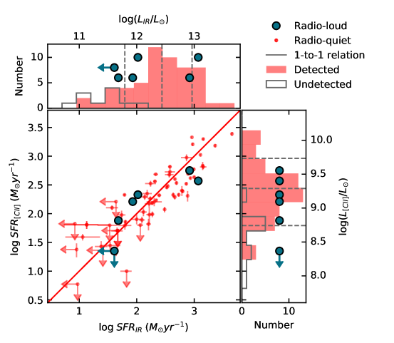
Figure 8: Star-formation distributions for radio-quiet (small points) and radio-loud (circles) quasars at $z\gtrsim 6$, derived from [C ii] and IR luminosities (Figure adapted from Khusanova et al. 2022).

The radiation at observed far-IR (FIR) to mm wavelengths of $z\gtrsim 6$ quasars is dominated by the reprocessed emission from cool/warm dust in the host galaxy. These wavelengths provide the best window to study host galaxy properties, minimizing contamination from the quasar’s accretion disk emission. Pioneering works pushed the limits of mm and radio facilities to characterize the dust and the molecular and atomic gas in the first bright $z\gtrsim 6$ quasars discovered (e.g., Bertoldi et al. 2003, Walter et al. 2003, Maiolino et al. 2005, Beelen et al. 2006, Wang et al. 2007, 2008). These studies were only sensitive to the most luminous systems, and found that about 1/3 of high redshift quasar host galaxies have luminosity comparable to those of hyper-luminous IR galaxies ($L_{\rm FIR}\sim 10^{13}$ L_⊙). Assuming the dust heating came from starburst activity, this suggested enormous star formation rates of $100-1000\,M_{\odot}\,\rm yr^{-1}$. Therefore, these early studies showed that early SMBH growth can be accompanied by extended, intense star formation and large reservoirs of dense and enriched molecular gas.

Rapid progress has been made in FIR observations of high-redshift quasar host galaxies with the advent of ALMA and major upgrades on the NOEMA interferometers (conveniently located in different hemispheres). The greatest advances can be divided into three major areas: (i) sensitivity, (ii) resolution, (iii) multi-line tracers of the ISM.

Sensitivity: The $\text{[C\,{ii]}}_{158\,\mu\text{m}}$  fine-structure line, which is the primary coolant of the cold neutral atomic medium, has become the workhorse for studies of $z\gtrsim 6$ quasar hosts. This was the natural choice as [C ii] is one of the brightest emission lines in star-forming galaxies and its frequency at $z>6$ is conveniently located in a high-transmission atmospheric window visible with ALMA and NOEMA. [C ii] detections using the early generation of interferometers were challenging. By the time of the review of Carilli & Walter (2013), there were only two $z\gtrsim 6$ quasars with [C ii] detections, while now that number is $\sim 80$. [C ii] line and IR continuum luminosities measurements provide independent estimates of SFR. Fig 8 shows a recent compilation of the [C ii] and IR luminosities and SFRs for $z\gtrsim 6$ quasar hosts.

Early ALMA results demonstrated its ability to study [C ii] emission from quasar hosts of both UV-bright and UV-faint $z\gtrsim 6$ quasars (Wang et al., 2013, Willott et al., 2013). These studies motivated the push to larger samples, marking the transition from studies of individual interesting sources to the first statistical samples. Decarli et al. (2018) and Venemans et al. (2018) presented results from an ALMA snapshot survey of a large sample of luminous $z\sim 6$ quasars to study their FIR continuum and [C ii] properties. Remarkably, even with integration time of $\lesssim 15$ min on ALMA, the detection rate is $\gtrsim 90$% for these quasars. They found typical [C ii] luminosities of $10^{9}-10^{10}\,L_{\odot}$, FIR luminosities of $0.3-13\times 10^{12}\,L_{\odot}$, and estimated dust masses of $10^{7}-10^{9}\,M_{\odot}$ with star formation rates ranging from 50 to 2700 $M_{\odot}$ yr^-1. ALMA also enabled detections of FIR continuum and [C ii] emission in a significant number of UV-faint quasars at high redshift (e.g., Izumi et al. 2018, 2019). Overall, there are only weak correlations between the bolometric luminosity of quasars (dominated by emission from accretion disk in the rest-frame UV/optical) and the FIR luminosity of the quasar hosts (dominated by star formation).

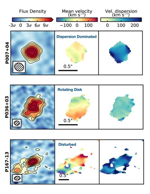
Figure 9: ALMA [C ii] observations of quasar hosts reveal diverse morphologies and kinematics (figure adapted from Neeleman et al. 2021). The top panel shows a dispersion dominated galaxy, the middle panel a galaxy consistent with a rotating disk, and the bottom panel shows a disturbed galaxy with an on-going merger.

Resolution: The unprecedented spatial resolution of ALMA allowed imaging of the ISM of $z>6$ quasar host galaxies at sub-kpc resolution for the first time. The first studies at kpc scales ($\sim 0.2-0.3^{\prime\prime}$) revealed interesting morphological characteristics. For example, Shao et al. (2017) found ordered motion in a $z=6.13$ host that can be modeled with a rotating disk, Venemans et al. (2017a) report a remarkably compact ($\lesssim 1\,$kpc) host galaxy at $z=7.08$ that does not exhibit ordered motion on kpc scales, and Bañados et al. (2019a) showed that a galaxy merger hosts a $z=7.54$ quasar.

Venemans et al. (2020) presented a survey of 27 host galaxies at $z\sim 6$ imaged at kpc scale with ALMA. They showed that the [C ii] emission in the bright, central regions of the quasars have sizes of 1.0–-4.8 kpc and are typically more extended than the dust continuum emission. The implied star formation rate densities at the center of these quasar hosts are a few hundred $M_{\odot}$ yr^-1 kpc^-2, below the Eddington limit for star formation (although there are examples of host galaxies forming stars at near the maximum possible rate, e.g., Andika et al. 2020, Yue et al. 2021b). Neeleman et al. (2021) modeled the kinematics of these 27 host galaxies. They found a large diversity in the quasar host properties. About 1/3 of the galaxies show smooth velocity gradients consistent with emission from a gaseous disk. About 1/3 have no evident velocity gradients, with their kinematics dominated by random motion. The final 1/3 exhibit signatures of close companion interaction or galaxy merger activities (see Fig. 9 for examples). The highest resolution observations that currently exist for $z>6$ quasars are 400 pc for a quasar host at $z=6.6$ (Venemans et al., 2019) and 200 pc for a host galaxy at $z=6.9$ (Walter et al., 2022). These two studies highlight the power of ALMA by revealing complex morphologies, [C ii] cavities in the gas distribution, and in one case very compact dust continuum and [C ii] emission, reaching extreme densities in the central 200 pc from the SMBH. We expect that observations at comparable resolution or higher will be an active area of investigation in the near future.

A key result of these morphological studies is that the population of host galaxies of luminous early quasars is diverse. While, on average, they are sites of massive galaxy assembly, they also appear to be in different evolutionary phases. Apparently, the peak of quasar activity is not tied to a particular stage of early galaxy formation in those systems.

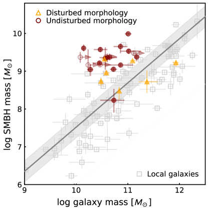
Figure 10: Black hole mass vs. host dynamical mass for $z\gtrsim 6$ quasars (figure from Neeleman et al. 2021). The gray points are local galaxies and the shaded region is the best-fit local relation (Kormendy & Ho, 2013). The $z\gtrsim 6$ sample is divided by their [C ii] morphology (see legend) and it is generally above the local relation.

Multi-line diagnostics: Even though the [C ii] emission line is important for redshift determination and gas dynamics (as discussed above), it cannot constrain the physics of the ISM by itself. A suite of emission lines tracing various phases of the ISM is required to characterize the physical conditions such as temperature, ionization, density, and metallicity. At the time of writing, this is an area of rapid development, and about a dozen quasar hosts have been detected in more than one tracer. Some of the main targeted lines (in addition to [C ii]) are:

• The neutral carbon emission [CI] 369 $\mu$m line, which traces the atomic medium in the external shells of molecular clouds (e.g., Yang et al., 2019a, Pensabene et al., 2021).

• Two transitions of the [NII] line (205 $\mu$m and 122 $\mu$m), which is a pure tracer of the ionized medium and can be used to measure the fraction of [C ii] associated with the neutral medium (e.g., Novak et al. 2019, Li et al. 2020).

• The [OI] 146 $\mu$m line, which is sensitive to the temperature of the atomic gas in the galaxy (e.g., Li et al. 2020, Meyer et al. 2022b).

• The [OIII] 88 $\mu$m line, which provides critical diagnostics for the conditions of star formation and the properties of massive stars (e.g., Walter et al. 2018, Hashimoto et al. 2019, Novak et al. 2019).

• Several rotational CO transitions: considered as the main probe of the molecular gas in dense star-forming regions (e.g., Gallerani et al., 2014, Venemans et al., 2017b, Novak et al., 2019, Decarli et al., 2022, Li et al., 2022b, Pensabene et al., 2021, Yang et al., 2019a)

• Several water lines that arise in the warm, dense phase of the interstellar medium and a number of OH molecular lines that are usually associated with outflows of dense material (e.g., Yang et al. 2019a, Pensabene et al. 2021, 2022).

A combination of these different tracers yields molecular gas masses in the range $M_{\rm H2}\sim 10^{10}-10^{11}\,M_{\odot}$, and ISM metallicities comparable to the solar value. Generally, the observed luminosities are better modeled by photo-dissociation regions instead of X-ray-dominated regions (see the review by Wolfire et al. 2022). The current small sample of quasars with multiple ISM tracers is highly biased towards objects bright in [C ii]. We expect that the characterization of physical conditions of the ISM in early massive galaxies will be expanded to much larger samples.

5.3 Constraints on Galaxy Mass and Black Hole/Galaxy Co-Evolution

Dynamical masses of the quasar hosts can be measured using spatially and kinematically resolved line observations (see Section 5.2). The dynamical mass enclosed within a radius $R$ is typically expressed as:

$$M_{\rm dyn}=\frac{v^{2}_{\rm circ}}{G}R,$$ (11)

where $G$ is the gravitational constant and $v_{\rm circ}$ is the maximum circular velocity of the gas disk. Obtaining $v_{\rm circ}$ is not trivial, as it requires knowing the inclination angle of the galaxy. Estimates of dynamical masses combined with robust BH masses (Section 4.1) make it feasible to push BH/galaxy co-evolution studies to the highest accessible redshifts.

Wang et al. (2010) measured dynamical masses using CO emission from 8 quasar hosts at $z\sim 6$. Assuming an average inclination angle of $40^{\circ}$ and $R=2.5\,$kpc, they found that the $z\sim 6$ quasars have, on average, SMBHs a factor 15 more massive than expected from the local BH – bulge mass relation. This result suggests that BHs in high redshift quasars either got a major head-start or grew faster than their host galaxies; if the M-$\sigma$ relation existed at $z\sim 6$, would show a strong cosmic evolution. Numerous subsequent works have focused on the correlation of SMBH mass and galaxy dynamical mass at these redshifts (e.g., Wang et al. 2016, Decarli et al. 2018). Most of these studies had to assume an inclination angle and/or an average size for the emitting gas. Neeleman et al. (2021) carried out careful dynamic modeling of their [C ii] observations (including inclination and size). They found a mean dynamical mass of $\sim 5\times 10^{10}$ M_⊙ for a sample of luminous $z\sim 6$ quasars with $\sim 10^{9}$ M_⊙ BHs. As shown in Fig. 10, this places them about one order of magnitude above the local relation. It is important to note that the relationship could be strongly affected by potential biases from selection and by using gas tracers (Huang et al. 2018, Volonteri & Stark 2011). Indeed, observations of low luminosity quasars show a narrower [C ii] line width (e.g., Willott et al. 2017, Izumi et al. 2018), placing them close to the local relation.

Habouzit et al. (2022) analyzed the co-evolution of SMBHs and their host galaxies in six cosmological simulations with different models for SMBH growth. Although the simulations are all consistent at $z\sim 0$, they diverge at $z>5$, highlighting the importance of obtaining robust observational constraints at these redshifts. Li et al. (2022a) argued that to robustly confirm whether the highest-redshift quasar population resides above the local BH - bulge mass relation, an improvement in the accuracy of mass measurements and an expansion of the current sample to lower black hole masses is required. We expect that JWST will enable significant advances for BH and galaxy host masses.

5.4 Evidence of Quasar Feedback

Central accreting SMBHs play an important role in shaping galaxy evolution (see review by Fabian, 2012). Indeed, to reproduce the observed distribution of galaxy masses at $z=0$, simulations require that strong AGN feedback was already in place at $z\sim 6$ (e.g., Kaviraj et al. 2017). Below we list some of the observational evidence (with caveats) that these feedback mechanisms are taking place in the $z\gtrsim 6$ quasar population:

UV Line Shifts. High-redshift quasars show asymmetric shape and velocity offset of high ionization lines, in particular the C iv line. The low-redshift quasar population shows an overall blueshifted C iv line ($\sim 800$ km s^-1) compared to the systemic redshift of the quasar (e.g., traced by H$\beta$, Shen et al., 2011). This shift is generally understood in the context of a strong accretion disk wind that contributes to the high-ionization lines (e.g., Richards et al., 2011). At $z>6$, the C iv line velocity shift is much stronger ($\sim$ 1800 km s^-1, Schindler et al., 2020). Meyer et al. (2019) suggested that this redshift evolution can be explained by the C iv winds being launched from the disk with an increased torus opacity at this redshift.

BAL Quasars. A fraction of quasars show broad and highly blue-shifted absorption features in their rest-frame UV transitions. BAL features trace ionized winds in the broad line region and are recognized signatures of SMBH feedback. Bischetti et al. (2022) used high-quality spectra of quasars from the XQR30 survey to show that up to $\sim 50\%$ of luminous quasars at $z\sim 6$ exhibit BAL features (with outflow velocities up to 17% of the speed of light), compared to about 20% observed in low-redshift samples. Yang et al. (2021) studied 37 quasars at $6.3<z<7.64$ and reported a BAL fraction of $\sim 24\%$, smaller than the Bischetti et al. (2022) work but still slightly larger than what is observed at lower redshifts. This potential evolution of the BAL fraction could be a result of the strong feedback associated with the rapid BH growth and galaxy assembly in the early Universe.

Ly$\alpha$ halos. The existence of extended $\text{Ly}\alpha$ nebulae around $z\gtrsim 6$ quasars was discussed in Section 5.1. Recently, Costa et al. (2022) performed a suite of cosmological, radiation-hydrodynamic simulations to understand the origin and properties of the observed Ly$\alpha$ halos. The simulations unambiguously require quasar-powered outflows to match the observed properties at $z\gtrsim 6$, providing indirect evidence for AGN feedback.

Radio jets. Only six galaxies hosting radio-loud quasars at $z\gtrsim 6$ have been studied with ALMA and NOEMA (Rojas-Ruiz et al. 2021, Khusanova et al. 2022). Assuming no AGN contribution, their, their [C ii]- and FIR-derived star-formation properties are consistent with those reported for the much more studied radio-quiet quasars (c.f., Decarli et al. 2018, Venemans et al. 2020; see Fig. 8). However, Rojas-Ruiz et al. (2021) and Khusanova et al. (2022) show indirect evidence that the FIR emission of radio-loud quasars can be strongly affected by synchrotron emission. In that case, their IR-derived star formation rates can be overestimated, implying that we might be witnessing negative AGN feedback at $z>6$. However, more measurements of the FIR continuum and/or an enlarged sample are required to quantify the potential impact on the population.

Broad components of [CII] emission. Broad wings ($\gtrsim 1000\,{\rm\,km\,s^{-1}}$) in the [C ii] emission lines are thought to be caused by AGN outflows. The observational evidence for these [C ii] broad wings remain tentative, as different analyses of similar datasets provide inconsistent results. For example, Maiolino et al. (2012) and Cicone et al. (2015) reported a strong [C ii] outflow in the host galaxy of the quasar J1148+5251 at $z=6.42$. Meyer et al. (2022b), on the other hand, found no evidence of a broad velocity component but reported that J1148+5251 has the most spatially extended [C ii] emission ($\sim 10\,$kpc) among $z\sim 6$ quasar hosts. Izumi et al. (2021) report a broad ($\sim 1000\,{\rm\,km\,s^{-1}}$) [C ii] wing in the spectrum of a quasar at $z=7.07$, and Khusanova et al. (2022) reported a tentative [C ii] broad component that could be as wide as $\sim 1400{\rm\,km\,s^{-1}}$ in a BAL radio-loud quasar at $z=6.12$. Bischetti et al. (2019) stacked the [C ii] spectra of 48 quasars at $4.5<z<7.1$ and reported a broad [C ii] component, while Decarli et al. (2018) stacked the [C ii] spectra of 23 $z\sim 6$ quasar hosts and found no evidence for a [C ii] broad component. Novak et al. (2020) stacked the [C ii] spectra using different techniques (spectral stacking and $uv$-plane stacking) and found no evidence for [C ii] broad-line emission. Novak et al. (2020) argued that the results can depend on the stacking techniques and resolution (e.g., if the resolution is low nearby companions can be confused with [C ii] wings).

OH absorption. The hydroxyl molecule (OH) in absorption traces high-velocity molecular inflow or outflows (see review by Veilleux et al. 2020). Herrera-Camus et al. (2020) report the first tentative detection ($3\sigma$) of the OH 119 $\mu$m doublet in absorption towards a $z\gtrsim 6$ quasar, suggesting the presence of a molecular outflow. Outflow signatures from both atomic and molecular lines will be a focus of future high-quality ALMA observations.

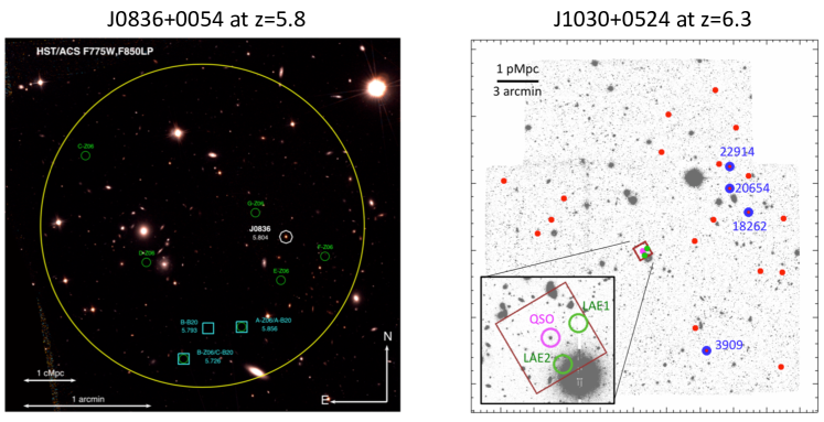
Figure 11: The two $z\gtrsim 6$ quasars with robust overdensities on $\gtrsim 1$ Mpc scales. Left: Field around J0836+0054 at $z=5.8$ (figure from Overzier 2022). Cyan squares (green circles) show spectroscopically-confirmed (photometrically-selected) galaxies at a redshift consistent with the quasar. Right: Field around J1030+0524 at $z=6.3$ (figure from Mignoli et al. 2020). Red dots show photometrically selected galaxies at a redshift consistent with the quasar. Blue and green circles are spectroscopically confirmed galaxies at a redshift consistent with the quasar.

5.5 Protoclusters and Large Scale Structure

Theoretical models predict that $z\gtrsim 6$ quasars should be highly biased tracers of the underlying dark matter distribution, signposting the first overdensities of galaxies on Mpc scales, i.e., protoclusters (e.g., Overzier et al. 2009, Costa et al. 2014; but some scatter is expected, see e.g., Ren et al. 2021). Observationally, this has been challenging to demonstrate. Photometric selection around high-redshift quasars has found evidence for overdensities (e.g., Utsumi et al., 2010, Morselli et al., 2014), densities comparable to random fields (e.g., Bañados et al., 2013, Simpson et al., 2014, Mazzucchelli et al., 2017a), and even underdensities (e.g., Kim et al., 2009).

There are currently two $z\gtrsim 6$ quasar fields with robust overdensities (i.e., including spectroscopic confirmation) on Mpc scales (Overzier 2022, Mignoli et al. 2020; see Fig. 11). These are SDSS J1030+0524 at $z=6.3$ and SDSS J0836+0054 at $z=5.8$. The works by Stiavelli et al. (2005), Kim et al. (2009), Simpson et al. (2014), Balmaverde et al. (2017), Decarli et al. (2019b) were crucial for confirming the overdense environment of J1030+0524. Similarly, Zheng et al. (2006), Ajiki et al. (2006), Bosman et al. (2020) were fundamental for confirming the large-scale structure around J0836+0054. Recently, Yue et al. (2021a) report the first quasar pair known at $z\sim 6$ (with a projected separation $<10\,$kpc), implying a rich environment that still awaits confirmation at larger scales.

ALMA observations of $z\sim 6$ quasars hosts (see Section 5.2) have serendipitously detected a population of [C ii]-bright companion galaxies in the immediate environment of $\sim$20-50% of the targeted quasars (Decarli et al. 2017, Neeleman et al. 2019, Venemans et al. 2020; see also bottom panel of Fig. 9). The large fraction of such quasar-galaxy pairs exceeds by orders of magnitude the expectations based on the current constraints of the number density of [C ii]-bright galaxies at these redshifts. Three out of five quasar companions with deep HST observations remain undetected (Mazzucchelli et al., 2019, Decarli et al., 2019a), implying a significant part of a potential large-scale structure might be obscured. The two HST-detected companions show tentative evidence of AGN activity (Connor et al. 2019, Vito et al. 2019b; but see also Vito et al. 2021).

The field of view of ALMA is too small to study whether these gas-rich companions exist in large numbers over Mpc scales as predicted by simulations. MUSE observations of one of these quasar/companion fields reveal two additional LAEs in close proximity, strengthening the case for an overdensity (Meyer et al., 2022a). It is likely that the next leap on our understanding of the environment of the highest-redshift quasars will come with JWST. JWST deep imaging, multi-object, and slitless spectroscopy capabilities will provide a new opportunity to probe the galaxy population in $z\gtrsim 6$ quasar environments to unprecedented depth over the Mpc scales.

6 QUASARS AS PROBES OF COSMIC REIONIZATION

Quasars are both agents, and powerful probes of the cosmic reionization history. As rare but luminous sources with hard ionizing spectra, they contribute to the overall photon budget driving reionization, together with stellar photons from galaxies. Absorption measured in quasar spectra from foreground gas has yielded many of the most sensitive constraints on the density, ionization, and chemical enrichment of this tenuous intergalactic material. While quasars’ utility as reionization probes has been understood since foundational work by Gunn & Peterson (1965), it has taken 40-50 years for quasar surveys to uncover objects deep into the reionization epoch and fully exploit the information that their absorption spectra encode (Fan et al., 2006b).

While absorption studies have yielded many of the most precise constraints on the IGM opacity and neutral hydrogen fraction, they are subject to limitations on both systematic accuracy, and physical interpretation. These limitations arise from multiple sources, but the most significant factors discussed below are (a) uncertainty in the quasar’s intrinsic/unabsorbed spectral continuum, (b) the large on-resonance oscillator strength of H i $\text{Ly}\alpha$, which leads to a wide gap in sensitivity between neutral fractions of $X_{\text{H\,{i}}}\sim 10^{-4}$ (where resonance absorption saturates) and $\sim 10^{-1}$ (where damping wings appear), and (c) computational challenges of simulating representative volumes with inhomogeneous and rapidly evolving radiation fields.

6.1 AGN and the Ionizing Photon Budget

Quasar accretion produces a hard ionizing spectrum, making the AGN population a contributing source to the budget of photons needed for reionization. However as detailed in the recent review by Robertson (2021) and references therein, there is an emerging consensus that AGN play a subdominant role compared to galaxies as an overall driver of the phase transition, even when one extrapolates observed luminosity functions to thresholds fainter than current detection limits. Jiang et al. (2022) further reinforced this conclusion by placing an upper limit on the contributions of low luminosity AGN to reionization using deep HST survey data. Finkelstein & Bagley (2022) have synthesized measurements across the lierature of galaxy+AGN UV luminosity functions, to estimate their relative contributions to the ionizing photon budget, using strong assumptions about the ionizing radiation escape fractions of each population. They estimate that AGN supply $\sim 10\%$ of the total ionizing photon budget at $z\sim 5$, roughly the lower limit of redshifts considered in our review. They found that this fraction drops rapidly toward higher redshift because of differential downward evolution in the quasar luminosity function relative to galaxies. By $z\sim 7$ they estimate that AGN contribute only $0.3-1.0\%$ of all ionizing photons, declining by yet another order of magnitude by $z\sim 9$. In contrast, Giallongo et al. (2019) suggested that AGN contributions to the UV background can still be significant at $z\sim 5.6$ based on X-ray selected objects.

The quantitative uncertainties in these analyses are still considerable; Finkelstein et al. (2019) found a $10\times$ higher contribution from AGN at $z\sim 7$ using different assumptions. Much of this may be attributed to uncertainties in the faint end slope of the quasar luminosity function. Still, the qualitative picture that reionization is heavily dominated by star-forming galaxies appears to remain fairly robust with respect to these uncertainties. The fractional contribution of quasars and AGN increases toward lower redshift because of their rapidly rising number densities, such that they are more likely to dominate the meta-galactic UV background in the at $z<4$ post-reionization universe. New surveys with the Nancy Grace Roman Space Telescope and JWST should revolutionize this field, providing both deep, near-IR color selected objects deep into the EoR, and also sensitive spectra to confirm the AGN nature of faint candidates and separate them from star-forming galaxies.

6.2 Neutral Hydrogen Absorption in the Diffuse IGM

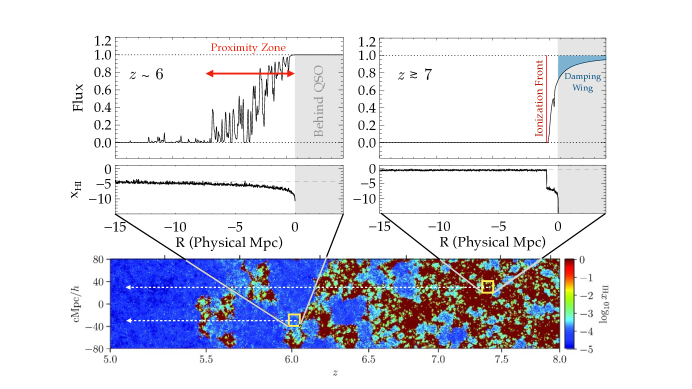
Figure 12: Observable properties and interpretation of Proximity Zones (upper left) and Damping Wings (upper right). In the simulation panel (bottom), each box represents the location of a background quasar whose sightline extends to the left. Proximity zones are studied at $z\sim 5.8-6.5$ and represent regions of enhanced ionization from the quasar in an already-ionized IGM. There is no absorption redward of the quasar’s Ly$\alpha$ emission line (marked with a gray shaded region), and a region of low optical depth extends $R_{p}\sim 5-10$ proper Mpc. Damping wings have only been detected at $z\gtrsim 7$, and represent ionization fronts penetrating into an IGM with a $O(\sim 0.1)$ neutral fraction, shown with red color scale in the simulation. On-resonance absorption is saturated up to and very near the quasar’s emission redshift, and the off-resonance Damping Wing (shaded blue) extends redward of Ly$\alpha$ in the quasar’s rest frame. Constraints on the IGM neutral fraction come from this blue shaded zone, as well as the very short run of unsaturated pixels between the QSO’s systemic redshift and the end of the proximity zone.

The optical depth from neutral Hydrogen in a matter-dominated universe (appropriate for the redshifts considered here) is:

$$\tau(\lambda_{obs})={{\pi e^{2}f_{\rm 12}}\over{m_{e}c}}\left({{{c}\over{H_{0}\Omega_{M}^{1/2}}}\int_{0}^{z}{{n_{\rm HI}(z)\over{(1+z)^{5/2}}}\phi(c/[\lambda_{0}(1+z)])dz}}\right)$$ (12)

The leading fraction has units of cross section per unit frequency in terms of the dimensionless oscillator strength $f_{12}$, which is an atomic constant determined for each ion ($f_{12}=0.416$ for Ly$\alpha$). The expression in brackets reflects a column density, i.e. an integral of the radial line element, weighted by the H i  density field. The function $\phi(\nu)$ is a unity-normalized line shape. It is typically approximated as a Voigt profile, which consists of a deep Gaussian line core whose width is determined by internal velocities, convolved with a much wider but also much weaker Lorentzian wing. This so-called “damping wing” arises from an energy-time uncertainty in the $\text{Ly}\alpha$ transition, leading to a small but non-zero absorption cross section in the rest frame for photons far from the resonance wavelength $\lambda_{\rm rest}=1215.67$ Å. Equation 12 indicates that the optical depth at each observed wavelength $\lambda_{\rm obs}$ contains contributions from neutral hydrogen at every intervening foreground redshift.

However because $\phi(\nu)$ is so sharply peaked around line resonance, the integral is almost always dominated by matter at the redshift where $\lambda_{\rm obs}/(1+z)=\lambda_{\rm rest}$. Directly at this resonance wavelength, the $\text{Ly}\alpha$ cross section is very large—roughly $4\times 10^{-14}$ cm². Moreover the mean baryonic density increases toward high redshift as

$$\bar{n}_{H}(z)\sim{{\Omega_{b}\rho_{c}}\over{\mu m_{H}}}(1+z)^{3}=8.6\times 10^{-5}\left({{1+z}\over{7}}\right)^{3}{\rm cm}^{-3},$$ (13)

which increases both the total gas column density, and also the H i  recombination rate, favoring a higher neutral gas fraction $X_{\text{H\,{i}}}$. Collectively these lead to a very large $\text{Ly}\alpha$ optical depth of $\tau\sim 10^{5}$ if the IGM is 100% neutral.

However, observations show $\tau=O(\sim 1)$ at $2<z<4$; the presence of transmitted flux implies that the $\text{Ly}\alpha$ forest is only neutral at the $X_{\text{H\,{i}}}\sim 10^{-5}$ level. The optical depth increases toward high redshift in tandem with the neutral fraction, but by the time the neutral fraction reaches $X_{\text{H\,{i}}}\sim 10^{-4}$, the optical depth already exceeds $\tau>5$, at which point $>99\%$ of the background quasar’s light is absorbed. On-resonance line absorption is simply too strong to provide useful measurements of the neutral fraction $X_{\text{H\,{i}}}$ above this value.

In contrast, the atomic cross section for a photon with wavelength in the Lorentzian damping wing is suppressed by 5–6 orders of magnitude relative to the peak at line center—even at small velocity offsets (100–200$\,{\rm\,km\,s^{-1}}$). The eponymous Damped Lyman Alpha (DLA) phenomenon is therefore only seen in small, rare high-overdensity environments with large column densities ($N_{\rm HI}>10^{20}$) at $z<5$.

Reionization is characterized by an increasing neutral fraction in the diffuse IGM, which eventually becomes strong enough to produce damping wings (Miralda-Escudé, 1998). However these are convolved with on-resonance absorption from H i at other redshifts, with the unique exception of the quasar’s immediate foreground, where the damping wing can extend redward of the $\text{Ly}\alpha$ emission line.

Bridging this gap between strong on-resonance absorption, whose measurements probe $10^{-6}<X_{\text{H\,{i}}}<10^{-4}$, and weak off-resonance damping wings which only emerge at $X_{\text{H\,{i}}}>10^{-1}$ is a recurring theme for IGM measurements near the reionization epoch. On-resonance measurements are most useful in regions of locally enhanced ionization or at lower redshifts ($z<6.3$) toward the late stages of reionization. Damping wing measurements are most powerful at early times and higher neutral fractions seen for $z>7$. Observational constraints are much less precise for the epochs in the range $6.3<z<6.8$, when the neutral fraction evolved from $0.01\%$ to $10\%$— the $\text{Ly}\alpha$ line absorption is saturated, but damping wings have not yet emerged.

6.2.1 Numerical Simulations

Cosmological simulations play an essential role in interpreting the spectra of reionization-epoch quasars, and placing their associated transmission measurements into a broader physical context. We refer the reader to an excellent recent review (Gnedin & Madau, 2022) on theoretical and numerical reionization models for a comprehensive overview of key methods and simulation projects.

Briefly, simulations must confront several intersecting challenges in the attempt to reproduce the quasar spectral observables summarized below, together with luminosity functions of reionization-era galaxy populations. An idealized simulation should have:

• A large box ($L>100$ cMpc) to cover many scale lengths of the galaxy-galaxy auto-correlation function, and to sample the rare high-density peaks that could plausibly host $M>10^{9}M_{\odot}$ SMBHs.

• Sufficient spatial and mass resolution to model disk galaxies realistically and resolve low-mass halos that produce light and heavy elements, as well as small-scale features in the $\text{Ly}\alpha$forest and Lyman Limit systems that act as ionizing radiation sinks.

• Ray tracing of emergent radiation from individual galaxies, to account for spatial variations in the density and ionizing background, shadowing from optically thick absorbers, or the timing of reionization.

• Full and self-consistent coupling of radiation to hydrodynamics, to capture the effect of ionization heating, pressure smoothing and adiabatic cooling on the evolving density field and ionization fraction. These will also impact the formation of subsequent stars and galaxies.

Computational limits prevent practical simulations from meeting all four these requirements simultaneously, though rapid progress in recent years has allowed some groups to progress from analytic or semi-numerical efforts to meet two or even three of the above bullets in single simulations. The Gnedin & Madau review contains a helpful classification of leading numerical projects according to their box sizes, hydro prescriptions, treatment of the UV background, and radiation-hydro coupling.

While most large-scale simulations focus on reproducing global reionization signals such as the volume-averaged neutral fraction, a separate numerical toolkit has evolved specifically to interpret observations of proximity zones (Sec 6.3.1) and damping wings (Sec 6.3.2) produced in the immediate foreground of luminous quasars.

These investigations begin with global simulations of the reionization-era IGM, and introduce the effect of a high-luminosity quasar by hand in the simulation volume. A large parent simulation is searched for high-mass halos ($M\geq 1-2\times 10^{11}M_{\odot}$) representative of hosts where SMBHs are first thought to form. A bright quasar is then inserted at the center of the halo, emitting ionizing photons with a luminosity scaled to the absolute 1450Å magnitude of known quasars, and extrapolated to the Lyman edge using carefully constructed template SEDs. The simulation is then evolved forward to follow expansion of the ionization front or proximity zone into the IGM. Multiple sightlines are drawn through the simulation box, terminating at the quasar’s host halo, and simulated transmission spectra are extracted using the density, temperature, ionization and velocity cubes.

This methodology has been adapted by several groups to place joint constraints on quasar lifetimes and the IGM neutral fraction at $z>7$ (Bolton et al., 2011, Keating et al., 2015, Davies et al., 2018b, Cen & Haiman, 2000), and to estimate the ages of $z\sim 6$ quasars from their proximity zone sizes (Eilers et al., 2017, Bolton & Haehnelt, 2007, Chen & Gnedin, 2021). In ionized proximity zones, the simulations can also be used to calibrate methods to reconstruct the fluctuating density field near the central host (Chen et al., 2022).

Essentially the simulations are used to generate statistical realizations of the matter distribution around massive quasar host halos, capturing non-linear physics and scale-dependent correlations in a way that analytic PDFs of the optical depth and/or excursion set formalism cannot accomplish.

A completely separate class of simulations is beginning to address challenging questions about heavy element enrichment of the early IGM and CGM (Keating et al., 2016), for comparison with observation of heavy element absorption in $z>6$ QSO spectra. These simulations rely on subgrid feedback prescriptions for metal production, which are then transported with standard hydro treatments as at lower redshift. Translation from metal abundances into observable column densities is more complicated than for HI, because the ionization balance of multi-level ions depends on the UV background at other, often harder energies than the Lyman edge. A notable early effort in multi-frequency treatment of an inhomogeneous background is the Technicolor Dawn simulation (Finlator et al., 2018), which tracks 24 separate frequencies and measures ionization balances of C IV and Si IV in the $z>5.5$ universe, though with a much smaller box size ($L\sim 12$ cMpc) than the aforementioned simulations designed to capture quasar host halos.

6.2.2 Transmission measurements

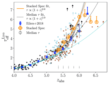
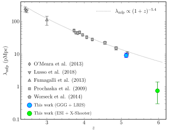
Figure 13: (Left): Evolution of the Ly$\alpha$ optical depth with redshift based on spectroscopy of large quasar samples, adapted from Yang et al. (2020a). The optical depth increases smoothly towards high redshift at $z<5.5$, then appears to evolve more strongly, with the emergence of complete Gunn-Peterson absorption troughs (upper limits). (Right) Evolution of the mean free path for ionizing photons, illustrating the rapid evolution approaching $z\sim 6$. Adapted from Becker et al. (2021).

Before the discovery of $z\gtrsim 6$ quasars, the evolving $\text{Ly}\alpha$ forest optical depth, which gradually increases with $z$, had been measured extensively at lower redshifts (Rauch et al., 1997, Becker et al., 2007) and interpreted as a product of the $\bar{n}\propto(1+z)^{3}$ density field together with a smoothly evolving UV ionizing radiation background (Becker & Bolton, 2013). Early discoveries of $z>6$ SDSS quasars (Fan et al., 2001) led to a reexamination of underlying assumptions about smooth evolution in $X_{\text{H\,{i}}}$ approaching reionization. In particular, deep medium-resolution spectroscopy of one of very first such objects — SDSS J1030+0524 at $z=6.3$ — revealed a region of Lya forest absorption consistent with zero flux at wavelengths corresponding to $5.95<z<6.16$ (Becker et al., 2001). This work has been interpreted as the first detection of a robust Gunn-Peterson absorption trough, and has been followed by many similar analyses to improve how the IGM opacity is quantified (Fan et al., 2006b, Yang et al., 2020a, Bosman et al., 2018, Eilers et al., 2018, Becker et al., 2007, Pentericci et al., 2002).

The simplest absorption indicator from a conceptual standpoint is the $\text{Ly}\alpha$ opacity, $\tau=-\ln(I/I_{0})$, where $I_{0}$ represents an estimate of the unabsorbed continuum flux level. Deeper spectra of SDSS J1030+0524 and many subsequently discovered objects consistently uncover similar spans of total absorption in $\text{Ly}\alpha$ resonance line at $z>6$, implying a large lower bound on $\tau$ limited only by the signal-to-noise ratio (SNR) of the spectral data. This highlights an important challenge in such measurements: the physical information is contained in measuring flux that is not seen. The logarithmic nature of optical depth means that even in spectra with SNR$\sim 100$ one can measure limits of $\tau\gtrsim 4$ (per pixel) at best, and the zero points can be affected by systematic errors in data reduction, including accurate subtraction night sky emission and correction for telluric absorption. Comparison of observations of the same quasars observed with different instruments and reduced with different pipelines indicate discrepancies at the 1–2% flux level, for a mean transmitted flux of 0.5–1.0% at $z\sim 6$ (McGreer et al., 2011, Eilers et al., 2018).

Additional dynamic range can often be achieved by observing Ly$\beta$ or higher order transitions from the Lyman series. These have progressively decreasing oscillator strengths and require correspondingly larger H icolumn to saturate, allowing access to larger values of $\tau$. This advantage is offset by complications arising from unknown blending with $\text{Ly}\alpha$ forest absorption at lower redshift, and uncertainty in extrapolating the intrinsic quasar continuum from $\text{Ly}\alpha$ to Ly$\beta$.

Measurements of the $\text{Ly}\alpha$ opacity are always smoothed to suppress noise and minimize the effect of differing spectral dispersion and resolution among instruments used in the observations. Following Fan et al. (2006b), most early studies have used observationally-motivated redshift bins of $\Delta z=0.15$ for ease of comparison, definining the ”effective optical depth” $\tau_{\rm eff}=-\ln\left<F\right>$ over the smoothing interval. More recent studies advocate for a physically-motivated bin size of 50 cMpc, because a constant redshift interval evolves by $\sim 40$% in comoving length over $5<z<7$ where such measurements are made (Eilers et al., 2018, Becker et al., 2015). The two values ($\Delta z=0.15$ and 50 cMpc) are comparable at $z\sim 7$. Fig 13 (left panel) presents a recent summary of $\text{Ly}\alpha$ optical depth measurements.

Average $\tau$ measurements are simply the first moment of an underlying optical depth distribution, which contains richer information and has therefore been measured extensively and presented as a cumulative distribution function (CDF) of optical depth. Evolution of the CDF is characterized by three phases, again reflecting the logarithmic nature of the measurements. At $z\sim 5.0-5.3$ the distribution is fairly narrow and centered around $\tau\sim 2$, corresponding to a $\text{Ly}\alpha$ forest with significant ($\sim 90\%$) absorption at line resonance, but not yet fully saturated. At $5.5<z<6.0$ the CDF widens to span $2<\tau<6$, as an increasing number of smoothed windows exhibit saturated absorption (i.e. zero transmitted flux or high $\tau$), but many significant transmission/low neutral fraction windows remain. Above $z>6$ it becomes increasingly rare to find unsaturated windows with $\tau<4$, and the distribution once again narrows because spectral SNR renders the $\tau>6$ regime inaccessible.

Several groups have explored alternative ionization metrics that use counts of transmission spikes in the Lya forest, motivated by the many challenges of measuring optical depths in realistic, heavily absorbed data. Garaldi et al. (2019) constructed distribution functions $d^{2}N/dLdz$, capturing the density of spikes per cMpc and unit redshift, above a threshold line flux. These can be counted in spectra of varying resolution and SNR using similar techniques as are used for blind searches for metal absorption lines in quasar spectra. Their analysis indicates that, after accounting for instrumental broadening and noise which suppress the spike count in realistic observed $5<z<6$ spectra by an order of magnitude, the observed spike counts are roughly consistent with their self-consistent simulations of the post-reionization IGM transmission. In the simulation boxes, transmission spikes arise from regions that are under-dense in hydrogen and galaxies, but over-ionized relative to expectations from equilibrium with the average radiation field, likely because of proximity to local ionizing sources.

At $z>6$ one expects transmission spikes to be exceedingly rare, so the detection even of single spikes implies the existence of early ionized cavities. Searches for spikes in high-redshift spectra have yielded several detections at $6<z<6.3$ that provide upper bounds on the local optical depth, complementing the lower bounds derived from measurements of saturated spectral regions (e.g., Yang et al., 2020a).

A very different way to conceptualize reionization is as a rapid increase in the mean-free-path (mfp) of ionizing photons. Although this is physically equivalent to an increase in the volume-averaged ionization fraction, this alternative framing allows a different analysis approach that does not require high-SNR measurements of localized pixels or spikes. Instead, samples of quasar spectra are stacked after shifting into the rest frame. Then a low-dimensional parametric model is fit to the shape of the stacked spectrum below the Lyman limit at $912$Å, corresponding to a probabilistic flight length of ionizing photons traveling from the quasar toward Earth. This model was originally developed at lower redshift to study the evolution of the ionizing background far from the background quasar. At high redshift, additional complexity must be added to the model to account for local ionization effects near the quasar, since the mean free path can approach the length scale of proximity zones of enhanced ionization around the quasar.

Fig 13 (right panel) presents the measurements of IGM mpfp using the most recent stacking analyses from Becker et al. (2021). It suggests a rapid change in the mean free path from $8-10$ pMpc at $z=5.1$ to $0.75-1.5$ pMpc at $z=6.0$ (the range reflects potential fluctuations from cosmic variance/sample size, and also uncertainty in the correlation between the H i opacity and ionization rate). This evolution is much stronger than would be inferred from extrapolation of the evolving mfp at lower redshifts, as one would expect in the late stages of a phase transition like reionization.

6.2.3 Dark Gaps and the late stages of reionization

The inverse phenomenon of $\text{Ly}\alpha$  transmission spikes—which trace the first environments to complete reionization at $z>6$—several quasar sightlines exhibit long, dark gaps of zero flux at $z<6$. These gaps are now understood to represent residual islands of neutral matter during late-stage reionization. As first explored by Becker et al. (2015) after the discovery of a $>110$ cMpc dark span towards the quasar ULAS J0148+0600, measurements of gap length have the advantage of being relatively insensitive to the details of estimating the quasar continuum, or absolute flux levels. Long gaps are not seen at $z\sim 5$, and indeed recent work by Zhu et al. (2021) finds that 90% of quasar spectra at $z\sim 6$ have a dark gap of 30 cMpc or longer, but only 15% do at $z=5.6$.

Gap statistics have generated significant theoretical interest, as they appear to be inconsistent with numerical models approximating the ionizing UV background field as spatially uniform at $z=5.5-6$ (Zhu et al., 2021). Various mechanisms have been proposed to explain the phenomenon, including (a) upward fluctuations in gas density (yielding a higher recombination rate and neutral fraction), (b) downward fluctuations in the ionizing radiation background, or (c) upward fluctuations in galaxy number density, leading to lower-than-average temperatures (D’Aloisio et al., 2015). The latter scenario is less intuitive, arising from a subtle effect where regions of high galaxy density reionize early, and then have more time to cool off from the associated photoionization heating. These first areas to reionize have a lower temperature than surrounding regions that reionize later and have not yet cooled. Because the H i recombination rate scales as $T^{-0.7}$, cooler regions that reionized earliest would have higher neutral fraction and opacity characteristic of dark gaps.

This yields a testable prediction to distinguish between dark gap models arising from UV background versus temperature-driven fluctuations (Davies et al., 2018a). Galaxy surveys along sightlines with gaps should see an enhancement in galaxy counts relative to the field if the gaps arise in cool regions that reionized early; conversely there should be a galaxy deficit if the gaps arise in islands of enhanced neutral fraction and/or low ionizing radiation background (two effects which are not straightforward to distinguish). Christenson et al. (2021), Becker et al. (2018), and Ishimoto et al. (2022) conducted narrowband Lya surveys in fields centered on well-known dark gaps to test this prediction, and found an underdensity of Lyman-alpha emitters within $20h^{-1}$ Mpc of the quasar sightline, favoring a scenario where the dark gaps represent residual neutral islands persisting in the late-reionization universe. Spectroscopic galaxy surveys have been difficult and expensive at these redshifts from the ground, but early observations with JWST indicate that prospects are very favorable for correlating galaxies observed in rest-frame optical emission lines with the IGM Lya opacity.

Overall, a consistent picture emerges from a suite of distinct IGM observations using quasar spectra, including (a) the average $\text{Ly}\alpha$ optical depth and its CDF, (b) dark gaps, (c) transmission spikes, and (d) the mean free path. The first three of these four measurements result from on-resonance $\text{Ly}\alpha$ absorption and the fourth measures the Lyman continuum, making them all most useful toward the tail end of reionization at $5.5<z<6.3$, when the volume-averaged neutral fraction is $\sim 10^{-4}$, but with significant spatial fluctuations. Taken together there is evidence that large neutral islands persisted well after $z\sim 6$, possibly in regions of low galaxy density and ambient ionizing radiation. During this time there was a tenfold increase in the mean free path for ionizing photons, eventually reaching cosmological length scales of 10 pMpc or more. The earliest regions to fully reionize can be traced by transmission spikes at $z\sim 6.3$, and are likely to reside in regions of low gas density that happen by chance to fall near a source of ionizing radiation.

6.2.4 Thermal signatures

Ionizing sources emit a spectrum of radiation including photons with energy above the $E>13.6$ eV Hydrogen ionization potential. The excess photon energy heats the post-reionization IGM, which subsequently cools over time due to adiabatic cosmic expansion. Such heating and cooling is clearly seen during the reionization of He ii at lower redshift (Walther et al., 2019); an even larger effect should be present for Hydrogen reionization. Unfortunately unlike He ii, it is not possible to measure heating from Hydrogen reionization in “real time”, because Gunn-Peterson absorption fully blankets the signal at the redshifts of interest. Nevertheless the temperature of the IGM at lower redshift—after reionization is complete—still encodes information about the past thermal history.

High-resolution quasar spectra are excellent thermometers of the IGM, because thermal gas motions projected along the line of sight smooth or broaden absorption features. At lower redshifts where individual unblended lines can be resolved in the $\text{Ly}\alpha$ forest, temperature maps directly to line profile width through the Voigt profile parameter $b=\sqrt{2kT/m_{\rm ion}}$, though this signature is convolved with similar broadening from turbulence and bulk gas motions.

At $z>4.5$ it becomes impossible to distinguish individual lines, so the IGM’s temperature signal must be measured statistically. Effectively, thermal effects impose a low-pass filter on the power spectrum, smoothing out small scale structure in the pattern of $\text{Ly}\alpha$ transmission. The band limit of this filter is a partly a proxy for the instantaneous temperature, but it also retains a memory of past heating, which is partly manifested through a pressure (i.e. Jeans) broadening beyond the normal Hubble flow. These effects are calibrated by statistical comparison to cosmological simulations.

The simulations are generally run on a grid which varies the mean temperature of the IGM at specified redshifts $T_{0}(z)$, the slope $\gamma$ of the IGM’s temperature-density relation $T(\Delta)=T_{0}\Delta^{\gamma-1}$, and the thermal energy injected into the IGM during reionization $u_{0}$, in units of eV per baryon. Synthetic spectra are drawn directly from simulation volumes and run through identical analysis software as the true quasar spectra, to ascertain which combination of $T_{0},\gamma$ and $u_{0}$ produce 1D flux power spectra most closely matching observed values.

Using these methods, Boera et al. (2019) find IGM temperatures of $T_{0}=7000-8000$ K at $4.2<z<5.0$, which is where the effective optical depth of the forest is $1<\tau_{\rm eff}<2$, making the method most sensitive. Toward higher redshifts where Gunn-Peterson saturation begins to manifest, thermal measurements become increasingly challenging. However recent constraints have been extracted by fitting the widths of emission line spikes, indicating slightly higher $T_{0}=10,000-12,000$K at earlier times $z=5.3-5.9$ as expected according to the paradigm of heating and adiabatic cooling (Gaikwad et al., 2020).

The simulations can also explore a range of different reionization histories to see which parameters best reproduce the post-reionization power spectrum. Toy models of instantaneous reionization provide joint constraints on the redshift of thermal injection and its amplitude, favoring $z\sim 8-10$ as the reionization redshift, and peak post-reionization temperatures of $T=10,000-20,000$ K depending on the choice of ionizing background spectrum. Temperature constraints on the reionization history are limited because the IGM tends to rapidly cool back to its ionization equilibrium temperature, washing out the signal from the initial thermal impulse. As mentioned above, the rapid thermal broadening is accompanied by a pressure broadening that also manifests in the power spectrum, and is somewhat longer lived. It is not possible to fully disentangle pressure and temperature smoothing effects from line-of-sight measurements. However measurements made using pairs of adjacent quasar sightlines can break this degeneracy, since they only measure smoothing on a transverse spatial scale by construction (Rorai et al., 2017).

Summarizing, while the power spectrum and thermal history cannot provide precision constraints on the timing of hydrogen reionization, it supports a general result that by $z\sim 5$, the initial thermal energy injected into the IGM has already cooled substantially, by perhaps a factor of $2-3$. This sets a lower bound on the elapsed time between the period of thermal energy injection and $z\sim 4-5$ where the measurements are made. This in turn implies that the peak heating associated with reionization occurred at $7<z<10$, broadly consistent with CMB results reported by Planck (Planck Collaboration et al., 2020).

6.3 Neutral Hydrogen Absorption in the Quasar Environment

Each quasar spectrum offers the opportunity to study radiative feedback in the neighborhood of a luminous source of ionizing photons: the background object itself. At $2<z<3$, a clear deficit is seen in the density of Lyman alpha forest lines as a quasar’s emission redshift is approached (Murdoch et al., 1986, Bajtlik et al., 1988). For these lower redshifts where the ambient IGM is clearly optically thin, the so-called “proximity effect” reflects a local enhancement of ionization in an already highly-ionized medium, and can be used to derive estimates of the quasar’s ionizing flux over the metagalactic background.

This measurement becomes increasingly valuable at high redshift, because the diffuse IGM is optically thick to $\text{Ly}\alpha$  absorption. However the observational manifestation of interactions between quasar radiation and the IGM differs according to whether the surrounding medium has already undergone reionization — in which case one observes a “proximity zone” — or the surrounding medium still has a high neutral fraction — in which case one observes a damping wing. Both phenomena are now well established; in the sections below we aim to clarify the distinction between the two, reconcile some differences in definitions, and clarify at which redshifts each one is most powerful.

6.3.1 Proximity zones and the effects of quasar radiation on recently reionized matter

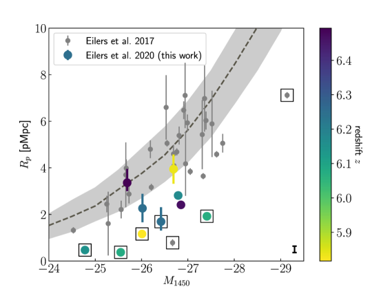
Figure 14: The size distribution of proximity zones at $5.9<z<6.4$ (Eilers et al., 2021), versus their host quasar’s absolute magnitude or luminosity. Shaded region shows expectations from a numerical simulation assuming the quasar has reached ionization equilibrium with its surroundings. This matches a representative sample of quasars at these redshifts (gray points), but separate samples have been identified with small proximity zones that have been interpreted as evidence of recent UV accretion episodes.

At $z_{\rm em}\sim 5.9-6.5$, on-resonance (Gunn-Peterson) $\text{Ly}\alpha$  has sufficient column density to fully absorb a quasar’s continuum. However the volume-averaged neutral fraction is only $\sim 10^{-4}$ during late-stage reionization, so a quasar’s local ionization boost can suppress the local $\text{Ly}\alpha$ opacity to optically thin values $\tau<1$, allowing some flux to transmit at wavelengths just blueward of the $\text{Ly}\alpha$ emission line. In exact analogy to the classic proximity effect at lower redshift, these “proximity zones” at $z\sim 6$ trace a local ionization enhancement in an already ionized medium. They should not be confused with Strömgren spheres, because the outside medium has a neutral fraction $X_{\text{H\,{i}}}\ll 1$.

The size of a quasar’s proximity zone depends on its ionizing photon luminosity, its lifetime (i.e. how long it has been shining in a UV-bright phase), and the density and ionization of the surrounding medium. By convention, observers have defined the proximity zone as the total path from $z_{em}$ to where a quasar’s spectral flux density remains $>10\%$ of the continuum level, after smoothing by a boxcar window of width 20Å  (Fan et al., 2006b). While observationally convenient and consistent, this definition is not motivated by any physical transition or process. It is loosely related to a radius of enhanced ionizing background, but at a 10% flux threshold the enhancement is still very strong — the quasar contribution exceeds the ambient field by an order of magnitude (Eilers et al., 2017). In select cases one may compare $\text{Ly}\alpha$ and Ly$\beta$ measurements to improve dynamic range in analogous fashion to IGM measurements (Mesinger & Haiman, 2004). In this case, one is probing the sharpness of the boundary of enhanced ionization fraction.

Uniformly selected samples have yielded typical proximity zone sizes of 2–6 pMpc, with a strong (expected) dependence on quasar luminosity, and comparatively weak dependence on redshift between $6.0<z<6.5$ (Eilers et al., 2017, 2020). Intriguingly, after adjusting proximity zone sizes to normalize out the effect of quasar luminosity, Eilers et al. (2017) found that $\sim 10\%$ of their sample had exceptionally small proximity zones. They argued that the most likely explanation is that we are observing these quasars before their radiation field has reached ionization equilibrium with the surrounding IGM, i.e. their current UV-luminous period is $t<100,000$ years old, with extreme objects even at $t<10,000$ years (Eilers et al., 2021). Stacking analysis of multiple quasars’ near zones indicates that the median quasar lifetime is larger by approximately an order of magnitude (Morey et al., 2021). Fig 14 presents a summary of proximity zone size measurements, along with “young quasars” identified through this type of measurement.

If this interpretation is correct, then proximity zone size distributions can be used to constrain the UV duty cycle of early quasars. The size is sensitive only to the age of the most recent or current UV-bright episode, which is not necessarily the first in its history. However the growth timescale problem for building SMBHs at $z>6$ is well known (see Sec 4; and Volonteri, 2010), and this challenge is only exacerbated for any accretion duty cycle below unity. It may be that the usual assumed correspondence between robust accretion and UV-bright episodes may need revision, and significant black hole growth can occur during a dusty, obscured phase.

6.3.2 IGM Damping Wings

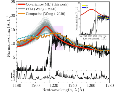
Figure 15: Damping wing measurements for J0252-0503 ($z=7.00$). Quasar spectrum is shows with black curve, and three continuum models are shown for the damping wing analysis. The quasars systemic redshift is shown with a vertical dashed line. Adapted from Greig et al. (2022).

As one penetrates deeper into the reionization epoch near $z\sim 7$, the ambient neutral fraction increases and the corresponding length scale of proximity zones becomes smaller. When the neutral fraction approaches 1–10%, the effects of off-resonance $\text{Ly}\alpha$ damping wings become significant (Miralda-Escudé, 1998). Details of this process have been reviewed in Mortlock (2016). Briefly, high column densities of neutral hydrogen in the nearby foreground of a quasar lead to a non-negligible probability that a photon emitted redward of $\text{Ly}\alpha$ in the quasar’s rest frame will still be absorbed by neutral intergalactic matter en route to Earth. This last fact is critical—in the far-foreground $\text{Ly}\alpha$ forest region there is an unresolvable degeneracy at any wavelength between off-resonance damping wing absorption from neutral gas, and on-resonance absorption from ionized gas at a different redshift. In contrast, absorption redward of the $\text{Ly}\alpha$ emission line can only come from off-resonance interactions.

The IGM damping signature is expected around quasars meeting two conditions: they have recently turned on, and are embedded in an IGM with high global neutral fraction. In contrast to $z\sim 6$ proximity zones that have already been pre-ionized by surrounding galaxies, the $z\sim 7$ quasars with damping wings are driving true ionization fronts into the surrounding IGM with a size that increases with the quasar’s active phase lifetime and ionizing photon flux, and decreases with larger overdensity.

The strength of a damping wing is most sensitive to the neutral fraction of matter just outside the quasar’s ionization front. Gas closer to the quasar is inside the ionization front, so its neutral fraction is too low to produce off-resonance $\text{Ly}\alpha$ absorption wings. Gas that is far outside the ionization front can produce off-resonance absorption, but its line-of-sight velocity offset is too large for the off-resonance wing to produce appreciable optical depth redward of Lya emission.

Damping wing measurements are significantly affected by systematic uncertainties in modeling the detailed shape of quasars’ intrinsic $\text{Ly}\alpha$ profile. Different groups have tackled this challenge using training sets of low-redshift SDSS or HST/COS spectra where the $\text{Ly}\alpha$ emission profile and unabsorbed continuum can be estimated more reliably. The objective is to predict the unabsorbed $\text{Ly}\alpha$ emission line shape and forest continuum (and associated uncertainties) using pixels to the red of the quasar’s $\text{Ly}\alpha$ emission line.

Multiple groups have used Principal Component Analysis (Davies et al., 2018c, Mortlock et al., 2011), Machine/Deep Learning models (Liu & Bordoloi, 2021), Neural Networks (Ďurovčíková et al., 2020), covariance matrices (Greig et al., 2017, 2022), stacking of nearest-neighbor observed spectra (Simcoe et al., 2012, Bosman & Becker, 2015, Bosman et al., 2021), or other hybrid approaches to train and validate continuum+$\text{Ly}\alpha$ software on lower redshift quasars. Most methods also calculate some envelope of formal uncertainty on the continuum estimate before applying them to $z\sim 7$ quasar spectra. When comparing different reconstruction techniques in the Ly$\alpha$/Ly$\beta$ forest region and around the $\text{Ly}\alpha$ emission line, the difference between continuum models for the same object using different codes often exceeds expectations from their formal error estimates, indicating the presence of residual systematics. It has therefore been important to test observations of the same objects taken using different instruments and analysis software to build confidence in the fundamental conclusion about damping wing strengths and the neutral fraction. Fig 15 illustrates some of the different techniques in predicting the quasar intrinsic spectrum in the damping wing region of a quasar at $z=7.0$.

While it is impossible to know if any particular continuum realization is “correct”, a consensus is indeed emerging that certain specific objects — most notably ULASJ1342+0928 ($z=7.54$; Bañados et al., 2018), DESJ0252$-$0503 ($z=7.00$; Wang et al., 2020), J1007+2115 ($z=7.51$; Yang et al., 2020b) and ULASJ1120+0641 ($z=7.09$; Mortlock et al., 2011) — show strong evidence for IGM damping wings for all continuum models explored in the literature. Various analyses derive slightly different IGM neutral fractions for the same objects on account of modeling differences (Greig et al., 2022, 2019, Davies et al., 2018b, Bolton et al., 2011). But a robust result remains that $67\%$ of known quasars at $z>7$ have (a) negligible proximity zone sizes, and (b) flux measurements at wavelengths slightly redder than the Lya emission line that fall below all continuum reconstructions based on low-redshift quasars. This combination of small proximity zone and damping wing has not been measured in a single quasar at $z<7$, despite the much larger sample sizes available for testing.

Because most of the damping wing is generated just outside the ionized bubble, there is a risk that the same signature could arise from chance alignment of a classical damped $\text{Ly}\alpha$ absorber (i.e. from the ISM of a bound proto-galaxy) near the quasar in an otherwise ionized IGM (Section 6.5). Indeed there are examples of such “proximate DLAs” in the literature, including several at $z>6$. The a priori odds of such a chance alignment are small, but were considered carefully in studies of the first damping wing (Simcoe et al., 2012). There are two arguments now suggesting that this phenomenon is not affecting IGM measurements at $z>7$. First, none of the four sightlines listed above exhibit heavy-element absorption at the redshift of the putative DLA, to very sensitive limits. Second, the presence of damping wings in multiple new $z>7$ discoveries points to a global phenomenon, as the joint probability of seeing proximate DLAs in all of these becomes lower still. With very high-SNR data it is in principle possible to distinguish between DLA absorption from the condensed CGM/ISM of a proto-galaxy and an extended patch of neutral but gravitationally unbound IGM using the damping profile alone. However no studies at present have claimed such a detection.

A final unknowable factor in damping wing analysis is the spatial distribution of gas density and accompanying fluctuations in ionization inside and outside the proximity zone. Early papers used analytic models based on distribution functions of overdensity, and assumed that the gas was in ionization equilibrium with a uniform background radiation field (Mortlock et al., 2011, Simcoe et al., 2012). Later and more sophisticated treatments have drawn distributions of sightlines from cosmological simulations to capture the line-of-sight variations in density and ionization (Greig et al., 2019). Large simulation boxes are required for this method, to identify the rare, high-mass halos where early quasars are thought to reside. Many sightlines are constructed which terminate by design at the high-mass halo, to generate many realizations of the damping wing for different viewing orientations.

Summarizing, among all quasar absorption methods, IGM damping wings yield the only two-sided constraint on $X_{\text{H\,{i}}}$ at $z>5.7$, and are therefore one of our most important probes of reionization history. They are nevertheless subject to substantial, and probably unresolvable systematic uncertainties concerning quasar continuum shape and details of the density and ionization fields around each quasar. Nevertheless a tentative consensus has emerged that for the majority of objects yet discovered at $7.0<z<7.5$, the near-zone size and damped absorption rule out models with global ionization fractions $X_{\text{H\,{i}}}<1\%$ or $X_{\text{H\,{i}}}\approx 100\%$, instead favoring values from $20-80\%$. Adding more objects will potentially increase confidence in the result, but may not reduce its fractional uncertainty to better than $\pm 40\%$, since the uncertainty envelope is dominated by model assumptions and is therefore not random.

Still this result is extremely significant because any measurement placing $X_{\text{H\,{i}}}\sim 50\%$ (or at a similar order of magnitude) represents a working definition of the reionization midpoint. Fig 16 summarizes the various reionization constraints from different quasar absorption observations, compared with both constraints from the measuremnts of CMB polarization (Robertson et al., 2015) and a number of empirical reionization history models. Optical depth measurements provide one-sided lower limits on $X_{\text{H\,{i}}}$ at $z<6.3$, transmission spikes provide one-sided upper limits at $5.5<z<6.5$, and damping wings provided two-sided constraints with large errors at $7<z<7.5$. This combination of limits and measurements permits models with a range of reionization histories with midpoints centered anywhere from $6.5<z<8.0$. Future 21-cm experiments will potentially measure these values with more precision and accuracy; these quasar constraints will help such experiments optimize their redshift window. Still, when expressed in terms of lookback time rather than redshift, quasar absorption constraints correspond to a 1–2% measurement of the timing of reionization, to $94.5^{+0.9}_{-0.5}$% lookback, or $760^{+80}_{-120}$ Myr after the Big Bang.

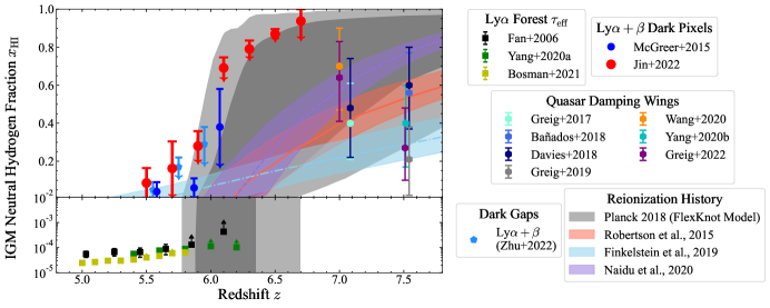
Figure 16: Summary of quasar absorption constraints on the reionization history (all data points; Figure adapted from Jin et al. 2022). The dark (light) gray-shaded region is the 1$\sigma$ (2$\sigma$) constraint from the Cosmic Microwave Background (Planck Collaboration et al., 2020). The red, blue, and purple shaded regions display the 1$\sigma$ reionization histories from the Robertson et al. (2015), Finkelstein et al. (2019), and Naidu et al. (2020) models, respectively. See Jin et al. (2022) and references therein, for more details.

6.4 Heavy Element Enrichment of Intervening Quasar Absorbers

The radiative feedback that drove reionization was accompanied by chemical feedback that can also be observed in the spectra of high redshift quasars. At $z>6$, large samples of high-resolution quasar spectra taken with VLT/XShooter, Magellan/FIRE, Keck/NIRES and Gemini/GNIRS have revealed foreground heavy element absorption lines redward of $\text{Ly}\alpha$  where the quasar’s continuum can be easily modeled. Because H i is saturated in the $\text{Ly}\alpha$ forest at $z>6$, metal absorption lines provide the only accessible information about diffuse gas at these epochs.

Absorption strength in these papers is sometimes reported as column density $N_{\rm ion}$ and other times as a rest-frame equivalent width $W_{r}$. The IR spectrographs listed above have intrinsic resolutions of $\Delta v\sim 50$ km/s or coarser, which is insufficient to resolve the fine $5-10$ km/s velocity structure seen in metal-line absorbers at lower redshift. Equivalent width measurements are therefore conservative and will be consistently measured across all spectrographs. Column densities are easier to interpret physically, but must be approached with care, accounting for the possibility of unresolved saturation in the line core, or blending of unresolved components. The detection sensitivity of current spectrographs limits metal line analyses to column densities characteristic of circumgalactic gas at lower redshift. Deeper spectra or statistical stacks will be needed to search for metals in the diffuse IGM.

Early studies of heavy element enrichment in the reionization epoch (Simcoe et al., 2011, D’Odorico et al., 2013, Ryan-Weber et al., 2006, Becker et al., 2009, Simcoe, 2006) focused on the C iv doublet, which is the most ubiquitous IGM metal line at lower redshifts and a tracer of highly-ionized circumgalactic gas. At $z>5.5$ C iv shifts into the $J$ band. Most surveys focus on a similar set of observables, including the comoving absorption density $dN/dX$, and the equivalent width distribution $d^{2}N/dXdW$.

These surveys established that the frequency of C iv absorbers decreases toward higher redshift, such that individual C iv systems become rare at $z>6$ — most sightlines have no C iv doublets in this range. For example, Codoreanu et al. (2018) surveyed deep spectra of four quasar sightlines, finding a four-fold decrease in comoving line density $dN/dX$ between $z=4.8$ and $z=5.7$, and zero detections above $z>6$, consistent with earlier but smaller studies in the literature (Simcoe et al., 2011). There is very tentative evidence of a steepening in the column density distribution function (CDDF) $f(N)=d^{2}N/dNdX$, because of differential evolution of the strongest C iv absorbers at high redshift. However these analyses still utilize modest numbers of sightlines ($<10$), so shot noise and saturation become significant limitations at the high-$W_{r}$ end. There are now relatively large samples of high quality spectra for $z>6.5$ quasars, which should lead to improved estimates of the CDDF and C iv evolution in the near future.

Evolving enrichment levels are sometimes summarized in terms of the C iv contribution to closure density $\Omega_{\rm CIV}$, which is a mass-weighted integral of the CDDF. Like $dN/dX$ or the normalization of $f(N)$, $\Omega_{\rm CIV}$ declines toward higher redshift. While it is convenient to express global metal enrichment in terms of this single number, the power-law slope $f(N)\propto N^{-1.5}$ of the CDDF is shallower than $\alpha=-2$, implying that the integral $\int Nf(N)dN$ diverges toward high column densities. The single strongest absorber in any sample therefore dominates the integral, meaning that by construction $\Omega_{\rm CIV}$ is affected by shot noise and pathlength searched.

The disappearance of C iv at high redshift could be driven either by a decline in heavy element abundances, or by a change in ionization. If abundance evolution predominates one might also expect to see a decline in the frequency of low-ionization species such as Mg ii, OI, SiII, CII, or FeII. However there have been robust detections of all these low-ionization lines at $z>6$, suggesting an important change in the ionization state of metal absorption line systems coincident with the reionization of intergalactic hydrogen.

The first detections of low-ionization metal absorption at $z>6$ focused on the OI 1302, CII 1334, and SiII 1260 lines, which have rest wavelengths only slightly to the red of $\text{Ly}\alpha$ and can therefore be detected in high-resolution optical (rather than infrared) spectra (Becker et al., 2011). However the small offset between these and $\text{Ly}\alpha$ also leaves a very short search pathlength per sightline; if they are too far in the quasar’s foreground these lines fall within the H i Gunn-Peterson trough and become impossible to detect.

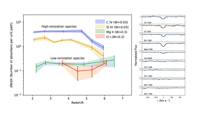
Figure 17: (Left) Evolution in number density $dN/dX$ of heavy element absorption systems, illustrating the different behavior between highly ionized species C iv and SiIV, which decline with increasing redshift, and low-ionization species Mg ii and OI, which do not decline. (Right) A stack of $z>5.7$ absorbers selected individually by MgII detection, which shows other low-ionization lines, but no evidence of C iv or SiIV.

With improved IR spectra it became possible to search systematically for low-ionization Mg ii doublets at $z>6$, albeit with complex selection windows caused by broadband atmospheric absorption between the $J/H$ and $H/K$ bands, discrete telluric absorption, and bright hydroxyl emission lines. After accounting for these effects, Mg ii surveys find trends consistent with the other neutral ions—there is no clear evolution in the comoving line density $dN/dX$ for systems with $W_{r}>0.3$Å (although if one restricts to very strong absorbers, there is a slight excess at $z\sim 3$; Chen et al., 2017, Matejek & Simcoe, 2012). Mg ii absorbers are now detected out to the highest known redshift of an absorption system, at $z=6.84$ (Simcoe et al., 2020).

The statistical decrease in C iv frequency together with statistical non-evolution of low-ionization species requires that as reionization is approached, one should eventually find individual absorbers with CII, OI, SiII, and Mg ii but no detection of a highly ionized C iv phase. This is indeed the case; in fact such low-ionization-only systems predominate at $z>6$, composing over 2/3 of all metal line absorbers (Cooper et al., 2019).

In sharp contrast, “low-ionization only” absorbers are exceedingly rare at all redshifts $z<5.5$, indicating a qualitative change in the CGM’s observable properties during the reionization epoch. At $2<z<4$ OI, CII, and SiII are much more rare than C iv; nearly every known low-ionization absorber is accompanied by stronger C iv and SiIV lines offset by $<100$ km/s, and there are many examples of C iv with no low-ionization lines (Cooper et al., 2019). Because absorption surveys are cross-section selected, the canonical interpretation is that ionized C iv traces a widespread low-density CGM, while OI, CII, and SiII trace cooled and condensed clumps in the ISM of a nearby galaxy, or small, cold precipitates embedded in the warm ionized CGM (Stern et al., 2016). The evolution of the number density of heavy element absorption systems is summarized in Fig 17.

The observational disappearance of the ionized CGM implies that during this epoch where galaxies are in early assembly, their circumgalactic gas has not yet been enriched to observable levels, and/or the ambient radiation field is insufficient in intensity or hardness to maintain a high degree of ionization. Unfortunately it is impossible to calculate abundances directly at $z>6$, because H i column density measurement is prevented by the Gunn-Peterson trough. However the number density of these low-ionization metal lines is similar to extrapolations of $dN/dX$ for DLAs and sub-DLAs (Cooper et al., 2019, Becker et al., 2019) and is either flat or slightly increasing at earlier times. If one assumes H i column densities in this range ($N_{\rm HI}>10^{19.8}$), the detected low-ionization lines are consistent with a metallicity of [C/H]$\sim-2.3$, in a warm neutral medium. If there exists a warm ionized medium of similar metallicity in pressure equilibrium with the warm neutral phase, it would be clearly detected in C iv. To evade detection, the ionized medium must have $\sim 100\times$ lower abundance, or [C/H]$<-4$ (Simcoe et al., 2020). If the heavy elements seen in low ionization lines are produced locally to that environment, this implies that those metals have not yet been mixed into the ionized CGM. Evidently the galactic environments traced by $z>6$ metal absorbers bear some resemblance to metal-poor DLAs at lower redshifts, but they are at an early and immature stage of chemical evolution and mixing.

6.5 Metal Absorption in the Vicinity of QSO Hosts

At all redshifts one can find a rare but important class of metal absorbers in the immediate foreground of their respective quasar hosts (Prochaska et al., 2008). These “proximate DLAs” have a special importance, and four have been discovered at $z>6$. They are the only discrete absorbers in the reionization epoch for which it is possible to constrain $N_{\rm HI}$ directly using the off-resonance wing. Because DLAs with $N_{\rm HI}>10^{20.3}$ cm^-3 are self-shielded and largely neutral, the pDLAs therefore also permit direct measurement of heavy element abundances, with no ionization correction needed.

The pDLAs are distinguished from IGM damping wings on the basis of coincident metal absorption. They are also found at lower redshift than the four $z>7$ IGM damping wing candidates—two pDLAs are at $z\sim 6.3-6.4$ (Bañados et al., 2019b, Andika et al., 2022), one at $z\sim 6$ (Davies, 2020), and one is at $z=5.93$, 40 kpc from a galaxy detected with ALMA at coincident redshift (D’Odorico et al., 2018). At these redshifts no other quasars have exhibited metal-free damping wings, and many observations of transmission spikes indicate that reionization is well underway (Yang et al., 2020a).

The pDLAs studied by Bañados et al. (2019b) and D’Odorico et al. (2018) have abundances near $0.001Z_{\odot}$, which would place them amongst the most metal poor DLAs known at lower redshift (Cooke et al., 2011). Neither shows evidence for anomalies in relative abundances, as might be expected from a medium enriched with Population III supernova debris. High ionization C iv and SiIV are not reported in either system, consistent with the discussion in the previous section about the disappearance of the high-ionization CGM phase. This has been cited as evidence that the pDLA originates outside of the quasar host, where the UV radiation field should be enhanced and an ionized medium would be expected.

The evidence so far suggests that pDLAs in the reionization epoch are representative of randomly intervening metal absorbers at similar redshift.

7 Summary

Since the first discoveries of reionization-era quasars more than twenty years ago, tremendous progress has been made in extending the frontiers of quasar research deeper into the cosmic dawn, in characterizing and understanding these objects in the context of early SMBH growth and galaxy formation, and in using them as beacons to shed light on the evolution of the IGM and the history of cosmic reionization.

[SUMMARY POINTS]

1. The current frontier of quasar research is at $z\sim 7.6$, with a large statistical sample assembled at redshifts up to 7. High-redshift quasar selection is a challenging data mining problem because of the rarity of the targets, the limited training sets, and the overwhelmingly large number of contaminant sources, both astrophysical and instrumental. We provide a database of the properties of all published quasars at $z>5.3$ as Supplementary Material that accompanies this review.

2. The rapid evolution of the quasar LF has been well established. However, the exact shape of the LF is still uncertain, both at the high luminosity end due to small number statistics, and at the low luminosity end due to limitations of deep surveys. In sharp contrast, early quasars “look” almost identical to their low-redshift counterparts in spectral properties. Even the earliest known quasars have a well-established AGN structure.

3. There are more than 100 $z\gtrsim 6$ quasars with robust BH mass measurements. Their masses range from $\sim$$4\times 10^{7}\,M_{\odot}$ to $\sim$$10^{10}\,M_{\odot}$. The BHs are growing at high Eddington ratios ($\lambda_{\rm Eff,median}=0.79$ and $\lambda_{\rm Eff,mean}=0.92$), with mild evidence of an increase of the accretion rate for $z\gtrsim 6.5$ quasars in comparison to luminosity-matched quasar samples at lower redshifts.

4. The UV stellar light in $z\sim 6$ quasar hosts remains undetected, while on the other hand, (sub)mm observations have revealed the existence of copious amounts of gas and cold dust in many of these galaxies. Quasar hosts are massive, star-forming galaxies showing diverse morphology and kinematics; their average dynamical mass appears lower than that based on the local scaling relation between BH and galaxy masses.

5. Ly$\alpha$ absorption in quasars’ foreground IGM provides many of the most stringent constraints on the history of reionization, though the details of the observations vary with redshift. Toward the end of reionization at $z<6$, counts of transmission spikes, dark gaps, and pixel optical depths indicate that universe is mostly ionized, but may harbor substantial islands of neutral matter as late as $z\sim 5.3$. At $z>7$, four quasars have been discovered with prominent, metal-free damping wings that are thought to represent off-resonance absorption from an IGM with neutral fraction $>10\%$, and possibly as high as $80\%$.

6. Heavy element absorption is seen in quasar spectra well into the epoch of reionization, tracing chemical feedback from stars whose radiation is also transforming the global ionization balance. It appears that these absorbers are high-redshift, low-metallicity analogs of damped Ly$\alpha$ absorbers observed at lower redshift. However the highly ionized phase of the circumgalactic medium, seen universally in CIV at $z<6$, abruptly vanishes in the EoR. This either indicates that the metals in the CGM are undergoing their own ionization transition, or that the ionized phase of the CGM has not yet been enriched with heavy elements at $z>6$.

[FUTURE ISSUES]

1. With the new facilities planned for the next decade, we expect the quasar redshift frontier to reach redshift 9–10, when the first generation of luminous quasars is forming. A key challenge will be the spectroscopic confirmation of these faint high-redshift sources.

2. SMBH mass measurements using the H$\beta$ line with JWST and gas-dynamical estimates with ALMA (and eventually the ngVLA) will provide more accurate measurements than what is currently possible. These results will be crucial to test whether the current methods calibrated at low redshift (e.g., Mg ii single-epoch virial mass) still hold at the highest accessible redshifts. To measure the BH masses of the progenitors of the currently observed $z=6-7$ quasar population, NIR spectroscopic follow-up with the ELTs will be key.

3. JWST will likely be able to finally reveal stellar light from $z\gtrsim 6$ quasar hosts. ALMA will continue playing a critical role in understanding and characterizing the interstellar medium of quasar host galaxies via multi-line diagnostics.

4. New quasar samples uncovered by Euclid and the Roman Space Telescope and observed with JWST and ELTs should substantially improve confidence in $z\geq 7$ measurements of IGM damping wings. They will allow studies even deeper into the past.

5. JWST already shows promise of being transformative for surveys of galaxies in fields where high-redshift quasars have been used to constrain the IGM density field. This may open the possibility of studying cross-correlations between $\text{Ly}\alpha$, metals, and galaxies.

DISCLOSURE STATEMENT

The authors are not aware of any affiliations, memberships, funding, or financial holdings that might be perceived as affecting the objectivity of this review.

References

- Abareshi et al. (2022) Abareshi B, Aguilar J, Ahlen S, Alam S, Alexander DM, et al. 2022. arXiv e-prints :arXiv:2205.10939
- Aihara et al. (2018) Aihara H, Armstrong R, Bickerton S, Bosch J, Coupon J, et al. 2018. PASJ 70:S8
- Ajiki et al. (2006) Ajiki M, Taniguchi Y, Murayama T, Shioya Y, Nagao T, et al. 2006. PASJ 58:499–502
- Andika et al. (2022) Andika IT, Jahnke K, Bañados E, Bosman SEI, Davies FB, et al. 2022. AJ 163(6):251
- Andika et al. (2020) Andika IT, Jahnke K, Onoue M, Bañados E, Mazzucchelli C, et al. 2020. ApJ 903(1):34
- Bañados et al. (2021) Bañados E, Mazzucchelli C, Momjian E, Eilers AC, Wang F, et al. 2021. ApJ 909(1):80
- Bañados et al. (2019a) Bañados E, Novak M, Neeleman M, Walter F, Decarli R, et al. 2019a. ApJ 881(1):L23
- Bañados et al. (2019b) Bañados E, Rauch M, Decarli R, Farina EP, Hennawi JF, et al. 2019b. ApJ 885(1):59
- Bañados et al. (2013) Bañados E, Venemans B, Walter F, Kurk J, Overzier R, Ouchi M. 2013. ApJ 773(2):178
- Bañados et al. (2016) Bañados E, Venemans BP, Decarli R, Farina EP, Mazzucchelli C, et al. 2016. ApJS 227(1):11
- Bañados et al. (2018) Bañados E, Venemans BP, Mazzucchelli C, Farina EP, Walter F, et al. 2018. Nature 553(7689):473–476
- Bañados et al. (2015) Bañados E, Venemans BP, Morganson E, Hodge J, Decarli R, et al. 2015. ApJ 804(2):118
- Bahk et al. (2019) Bahk H, Woo JH, Park D. 2019. ApJ 875(1):50
- Bajtlik et al. (1988) Bajtlik S, Duncan RC, Ostriker JP. 1988. ApJ 327:570
- Balmaverde et al. (2017) Balmaverde B, Gilli R, Mignoli M, Bolzonella M, Brusa M, et al. 2017. A&A 606:A23
- Barnett et al. (2021) Barnett R, Warren SJ, Cross NJG, Mortlock DJ, Fan X, et al. 2021. MNRAS 501(2):1663–1676
- Barnett et al. (2019) Barnett R, Warren SJ, Mortlock DJ, Cuby JG, Conselice C, et al. 2019. A&A 631:A85
- Barth et al. (2003) Barth AJ, Martini P, Nelson CH, Ho LC. 2003. ApJ 594(2):L95–L98
- Becker & Bolton (2013) Becker GD, Bolton JS. 2013. MNRAS 436(2):1023–1039
- Becker et al. (2015) Becker GD, Bolton JS, Madau P, Pettini M, Ryan-Weber EV, Venemans BP. 2015. MNRAS 447(4):3402–3419
- Becker et al. (2021) Becker GD, D’Aloisio A, Christenson HM, Zhu Y, Worseck G, Bolton JS. 2021. MNRAS 508(2):1853–1869
- Becker et al. (2018) Becker GD, Davies FB, Furlanetto SR, Malkan MA, Boera E, Douglass C. 2018. ApJ 863(1):92
- Becker et al. (2019) Becker GD, Pettini M, Rafelski M, D’Odorico V, Boera E, et al. 2019. ApJ 883(2):163
- Becker et al. (2007) Becker GD, Rauch M, Sargent WLW. 2007. ApJ 662(1):72–93
- Becker et al. (2009) Becker GD, Rauch M, Sargent WLW. 2009. ApJ 698(2):1010–1019
- Becker et al. (2011) Becker GD, Sargent WLW, Rauch M, Calverley AP. 2011. ApJ 735(2):93
- Becker et al. (2001) Becker RH, Fan X, White RL, Strauss MA, Narayanan VK, et al. 2001. AJ 122(6):2850–2857
- Beelen et al. (2006) Beelen A, Cox P, Benford DJ, Dowell CD, Kovács A, et al. 2006. ApJ 642(2):694–701
- Belladitta et al. (2020) Belladitta S, Moretti A, Caccianiga A, Spingola C, Severgnini P, et al. 2020. A&A 635:L7
- Bertoldi et al. (2003) Bertoldi F, Carilli CL, Cox P, Fan X, Strauss MA, et al. 2003. A&A 406:L55–L58
- Bischetti et al. (2022) Bischetti M, Feruglio C, D’Odorico V, Arav N, Bañados E, et al. 2022. Nature 605(7909):244–247
- Bischetti et al. (2019) Bischetti M, Maiolino R, Carniani S, Fiore F, Piconcelli E, Fluetsch A. 2019. A&A 630:A59
- Boera et al. (2019) Boera E, Becker GD, Bolton JS, Nasir F. 2019. ApJ 872(1):101
- Bolton & Haehnelt (2007) Bolton JS, Haehnelt MG. 2007. MNRAS 374(2):493–514
- Bolton et al. (2011) Bolton JS, Haehnelt MG, Warren SJ, Hewett PC, Mortlock DJ, et al. 2011. MNRAS 416(1):L70–L74
- Bosman & Becker (2015) Bosman SEI, Becker GD. 2015. MNRAS 452(2):1105–1111
- Bosman et al. (2018) Bosman SEI, Fan X, Jiang L, Reed S, Matsuoka Y, et al. 2018. MNRAS 479(1):1055–1076
- Bosman et al. (2020) Bosman SEI, Kakiichi K, Meyer RA, Gronke M, Laporte N, Ellis RS. 2020. ApJ 896(1):49
- Bosman et al. (2021) Bosman SEI, Ďurovčíková D, Davies FB, Eilers AC. 2021. MNRAS 503(2):2077–2096
- Boyle et al. (2000) Boyle BJ, Shanks T, Croom SM, Smith RJ, Miller L, et al. 2000. MNRAS 317(4):1014–1022
- Brandt et al. (2001) Brandt WN, Guainazzi M, Kaspi S, Fan X, Schneider DP, et al. 2001. AJ 121(2):591–597
- Carilli & Shao (2018) Carilli CL, Shao Y. 2018. Imaging Molecular Gas at High Redshift. In Science with a Next Generation Very Large Array, ed. E Murphy, vol. 517 of Astronomical Society of the Pacific Conference Series
- Carilli & Walter (2013) Carilli CL, Walter F. 2013. ARA&A 51(1):105–161
- Cen & Haiman (2000) Cen R, Haiman Z. 2000. ApJ 542(2):L75–L78
- Chambers et al. (2016) Chambers KC, Magnier EA, Metcalfe N, Flewelling HA, Huber ME, et al. 2016. arXiv e-prints :arXiv:1612.05560
- Chen et al. (2022) Chen H, Eilers AC, Bosman SEI, Gnedin NY, Fan X, et al. 2022. ApJ 931(1):29
- Chen & Gnedin (2021) Chen H, Gnedin NY. 2021. ApJ 911(1):60
- Chen et al. (2017) Chen SFS, Simcoe RA, Torrey P, Bañados E, Cooksey K, et al. 2017. ApJ 850(2):188
- Christenson et al. (2021) Christenson HM, Becker GD, Furlanetto SR, Davies FB, Malkan MA, et al. 2021. ApJ 923(1):87
- Cicone et al. (2015) Cicone C, Maiolino R, Gallerani S, Neri R, Ferrara A, et al. 2015. A&A 574:A14
- Codoreanu et al. (2018) Codoreanu A, Ryan-Weber EV, García LÁ, Crighton NHM, Becker G, et al. 2018. MNRAS 481(4):4940–4959
- Cohn et al. (2021) Cohn JH, Walsh JL, Boizelle BD, Barth AJ, Gebhardt K, et al. 2021. ApJ 919(2):77
- Connor et al. (2021) Connor T, Bañados E, Stern D, Carilli C, Fabian A, et al. 2021. ApJ 911(2):120
- Connor et al. (2019) Connor T, Bañados E, Stern D, Decarli R, Schindler JT, et al. 2019. ApJ 887(2):171
- Cooke et al. (2011) Cooke R, Pettini M, Steidel CC, Rudie GC, Nissen PE. 2011. MNRAS 417(2):1534–1558
- Cooper et al. (2019) Cooper TJ, Simcoe RA, Cooksey KL, Bordoloi R, Miller DR, et al. 2019. ApJ 882(2):77
- Costa et al. (2022) Costa T, Arrigoni Battaia F, Farina EP, Keating LC, Rosdahl J, Kimm T. 2022. arXiv e-prints :arXiv:2203.11232
- Costa et al. (2014) Costa T, Sijacki D, Trenti M, Haehnelt MG. 2014. MNRAS 439(2):2146–2174
- D’Aloisio et al. (2015) D’Aloisio A, McQuinn M, Trac H. 2015. ApJ 813(2):L38
- Davies (2020) Davies FB. 2020. MNRAS 494(2):2937–2947
- Davies et al. (2018a) Davies FB, Becker GD, Furlanetto SR. 2018a. ApJ 860(2):155
- Davies et al. (2018b) Davies FB, Hennawi JF, Bañados E, Lukić Z, Decarli R, et al. 2018b. ApJ 864(2):142
- Davies et al. (2018c) Davies FB, Hennawi JF, Bañados E, Simcoe RA, Decarli R, et al. 2018c. ApJ 864(2):143
- Davies et al. (2019) Davies FB, Hennawi JF, Eilers AC. 2019. ApJ 884(1):L19
- De Rosa et al. (2011) De Rosa G, Decarli R, Walter F, Fan X, Jiang L, et al. 2011. ApJ 739(2):56
- De Rosa et al. (2014) De Rosa G, Venemans BP, Decarli R, Gennaro M, Simcoe RA, et al. 2014. ApJ 790(2):145
- Decarli et al. (2019a) Decarli R, Dotti M, Bañados E, Farina EP, Walter F, et al. 2019a. ApJ 880(2):157
- Decarli et al. (2019b) Decarli R, Mignoli M, Gilli R, Balmaverde B, Brusa M, et al. 2019b. A&A 631:L10
- Decarli et al. (2022) Decarli R, Pensabene A, Venemans B, Walter F, Bañados E, et al. 2022. A&A 662:A60
- Decarli et al. (2017) Decarli R, Walter F, Venemans BP, Bañados E, Bertoldi F, et al. 2017. Nature 545(7655):457–461
- Decarli et al. (2018) Decarli R, Walter F, Venemans BP, Bañados E, Bertoldi F, et al. 2018. ApJ 854(2):97
- Decarli et al. (2012) Decarli R, Walter F, Yang Y, Carilli CL, Fan X, et al. 2012. ApJ 756(2):150
- Di Matteo et al. (2017) Di Matteo T, Croft RAC, Feng Y, Waters D, Wilkins S. 2017. MNRAS 467(4):4243–4251
- Diamond-Stanic et al. (2009) Diamond-Stanic AM, Fan X, Brandt WN, Shemmer O, Strauss MA, et al. 2009. ApJ 699(1):782–799
- D’Odorico et al. (2013) D’Odorico V, Cupani G, Cristiani S, Maiolino R, Molaro P, et al. 2013. MNRAS 435(2):1198–1232
- D’Odorico et al. (2018) D’Odorico V, Feruglio C, Ferrara A, Gallerani S, Pallottini A, et al. 2018. ApJ 863(2):L29
- Drake et al. (2019) Drake AB, Farina EP, Neeleman M, Walter F, Venemans B, et al. 2019. ApJ 881(2):131
- Drake et al. (2022) Drake AB, Neeleman M, Venemans BP, Novak M, Walter F, et al. 2022. ApJ 929(1):86
- Duras et al. (2020) Duras F, Bongiorno A, Ricci F, Piconcelli E, Shankar F, et al. 2020. A&A 636:A73
- Eddington (1926) Eddington AS. 1926. The Internal Constitution of the Stars
- Eilers et al. (2018) Eilers AC, Davies FB, Hennawi JF. 2018. ApJ 864(1):53
- Eilers et al. (2017) Eilers AC, Davies FB, Hennawi JF, Prochaska JX, Lukić Z, Mazzucchelli C. 2017. ApJ 840(1):24
- Eilers et al. (2021) Eilers AC, Hennawi JF, Davies FB, Simcoe RA. 2021. ApJ 917(1):38
- Eilers et al. (2020) Eilers AC, Hennawi JF, Decarli R, Davies FB, Venemans B, et al. 2020. ApJ 900(1):37
- Endsley et al. (2022) Endsley R, Stark DP, Lyu J, Wang F, Yang J, et al. 2022. arXiv e-prints :arXiv:2206.00018
- Fabian (2012) Fabian AC. 2012. ARA&A 50:455–489
- Fabian et al. (2014) Fabian AC, Walker SA, Celotti A, Ghisellini G, Mocz P, et al. 2014. MNRAS 442:L81–L84
- Fan (1999) Fan X. 1999. AJ 117(5):2528–2551
- Fan et al. (2019a) Fan X, Barth A, Banados E, De Rosa G, Decarli R, et al. 2019a. BAAS 51(3):121
- Fan et al. (2006a) Fan X, Carilli CL, Keating B. 2006a. ARA&A 44(1):415–462
- Fan et al. (2004) Fan X, Hennawi JF, Richards GT, Strauss MA, Schneider DP, et al. 2004. AJ 128(2):515–522
- Fan et al. (2001) Fan X, Narayanan VK, Lupton RH, Strauss MA, Knapp GR, et al. 2001. AJ 122(6):2833–2849
- Fan et al. (2006b) Fan X, Strauss MA, Becker RH, White RL, Gunn JE, et al. 2006b. AJ 132(1):117–136
- Fan et al. (1999) Fan X, Strauss MA, Schneider DP, Gunn JE, Lupton RH, et al. 1999. AJ 118(1):1–13
- Fan et al. (2019b) Fan X, Wang F, Yang J, Keeton CR, Yue M, et al. 2019b. ApJ 870(2):L11
- Farina et al. (2019) Farina EP, Arrigoni-Battaia F, Costa T, Walter F, Hennawi JF, et al. 2019. ApJ 887(2):196
- Farina et al. (2022) Farina EP, Schindler JT, Walter F, Bañados E, Davies FB, et al. 2022. arXiv e-prints :arXiv:2207.05113
- Finkelstein & Bagley (2022) Finkelstein SL, Bagley MB. 2022. arXiv e-prints :arXiv:2207.02233
- Finkelstein et al. (2019) Finkelstein SL, D’Aloisio A, Paardekooper JP, Ryan Russell J, Behroozi P, et al. 2019. ApJ 879(1):36
- Finlator et al. (2018) Finlator K, Keating L, Oppenheimer BD, Davé R, Zackrisson E. 2018. MNRAS 480(2):2628–2649
- Gaikwad et al. (2020) Gaikwad P, Rauch M, Haehnelt MG, Puchwein E, Bolton JS, et al. 2020. MNRAS 494(4):5091–5109
- Gallerani et al. (2014) Gallerani S, Ferrara A, Neri R, Maiolino R. 2014. MNRAS 445(3):2848–2853
- Garaldi et al. (2019) Garaldi E, Gnedin NY, Madau P. 2019. ApJ 876(1):31
- Ghisellini et al. (2014) Ghisellini G, Celotti A, Tavecchio F, Haardt F, Sbarrato T. 2014. MNRAS 438(3):2694–2700
- Giallongo et al. (2019) Giallongo E, Grazian A, Fiore F, Kodra D, Urrutia T, et al. 2019. ApJ 884(1):19
- Gloudemans et al. (2021) Gloudemans AJ, Duncan KJ, Röttgering HJA, Shimwell TW, Venemans BP, et al. 2021. A&A 656:A137
- Gnedin & Madau (2022) Gnedin NY, Madau P. 2022. arXiv e-prints :arXiv:2208.02260
- Goto et al. (2009) Goto T, Utsumi Y, Furusawa H, Miyazaki S, Komiyama Y. 2009. MNRAS 400(2):843–850
- Greig et al. (2019) Greig B, Mesinger A, Bañados E. 2019. MNRAS 484(4):5094–5101
- Greig et al. (2022) Greig B, Mesinger A, Davies FB, Wang F, Yang J, Hennawi JF. 2022. MNRAS 512(4):5390–5403
- Greig et al. (2017) Greig B, Mesinger A, Haiman Z, Simcoe RA. 2017. MNRAS 466(4):4239–4249
- Gunn & Peterson (1965) Gunn JE, Peterson BA. 1965. ApJ 142:1633–1636
- Habouzit et al. (2022) Habouzit M, Onoue M, Bañados E, Neeleman M, Anglés-Alcázar D, et al. 2022. MNRAS 511(3):3751–3767
- Haiman & Rees (2001) Haiman Z, Rees MJ. 2001. ApJ 556(1):87–92
- Hashimoto et al. (2019) Hashimoto T, Inoue AK, Tamura Y, Matsuo H, Mawatari K, Yamaguchi Y. 2019. PASJ 71(6):109
- Herrera-Camus et al. (2020) Herrera-Camus R, Sturm E, Graciá-Carpio J, Veilleux S, Shimizu T, et al. 2020. A&A 633:L4
- Hewett et al. (2006) Hewett PC, Warren SJ, Leggett SK, Hodgkin ST. 2006. MNRAS 367(2):454–468
- Hopkins et al. (2007) Hopkins PF, Richards GT, Hernquist L. 2007. ApJ 654(2):731–753
- Huang et al. (2018) Huang KW, Di Matteo T, Bhowmick AK, Feng Y, Ma CP. 2018. MNRAS 478(4):5063–5073
- Ighina et al. (2022) Ighina L, Moretti A, Tavecchio F, Caccianiga A, Belladitta S, et al. 2022. A&A 659:A93
- Inayoshi et al. (2020) Inayoshi K, Visbal E, Haiman Z. 2020. ARA&A 58:27–97
- Ishimoto et al. (2022) Ishimoto R, Kashikawa N, Kashino D, Ito K, Liang Y, et al. 2022. MNRAS 515(4):5914–5926
- Ivezić et al. (2019) Ivezić Ž, Kahn SM, Tyson JA, Abel B, Acosta E, et al. 2019. ApJ 873(2):111
- Iwamuro et al. (2004) Iwamuro F, Kimura M, Eto S, Maihara T, Motohara K, et al. 2004. ApJ 614(1):69–74
- Izumi et al. (2021) Izumi T, Matsuoka Y, Fujimoto S, Onoue M, Strauss MA, et al. 2021. ApJ 914(1):36
- Izumi et al. (2019) Izumi T, Onoue M, Matsuoka Y, Nagao T, Strauss MA, et al. 2019. PASJ 71(6):111
- Izumi et al. (2018) Izumi T, Onoue M, Shirakata H, Nagao T, Kohno K, et al. 2018. PASJ 70(3):36
- Jiang et al. (2009) Jiang L, Fan X, Bian F, Annis J, Chiu K, et al. 2009. AJ 138(1):305–311
- Jiang et al. (2010) Jiang L, Fan X, Brandt WN, Carilli CL, Egami E, et al. 2010. Nature 464(7287):380–383
- Jiang et al. (2006) Jiang L, Fan X, Hines DC, Shi Y, Vestergaard M, et al. 2006. AJ 132(5):2127–2134
- Jiang et al. (2007) Jiang L, Fan X, Vestergaard M, Kurk JD, Walter F, et al. 2007. AJ 134(3):1150
- Jiang et al. (2016) Jiang L, McGreer ID, Fan X, Strauss MA, Bañados E, et al. 2016. ApJ 833(2):222
- Jiang et al. (2022) Jiang L, Ning Y, Fan X, Ho LC, Luo B, et al. 2022. Nature Astronomy 6:850–856
- Jin et al. (2022) Jin X, Yang J, Fan X, Wang F, Bañados E, et al. 2022. arXiv e-prints :arXiv:2211.12613
- Jolley & Kuncic (2008) Jolley EJD, Kuncic Z. 2008. MNRAS 386(2):989–994
- Just et al. (2007) Just DW, Brandt WN, Shemmer O, Steffen AT, Schneider DP, et al. 2007. ApJ 665(2):1004–1022
- Kato et al. (2020) Kato N, Matsuoka Y, Onoue M, Koyama S, Toba Y, et al. 2020. PASJ 72(5):84
- Kaviraj et al. (2017) Kaviraj S, Laigle C, Kimm T, Devriendt JEG, Dubois Y, et al. 2017. MNRAS 467(4):4739–4752
- Keating et al. (2015) Keating LC, Haehnelt MG, Cantalupo S, Puchwein E. 2015. MNRAS 454(1):681–697
- Keating et al. (2016) Keating LC, Puchwein E, Haehnelt MG, Bird S, Bolton JS. 2016. MNRAS 461(1):606–626
- Khusanova et al. (2022) Khusanova Y, Bañados E, Mazzucchelli C, Rojas-Ruiz S, Momjian E, et al. 2022. A&A 664:A39
- Kim et al. (2009) Kim S, Stiavelli M, Trenti M, Pavlovsky CM, Djorgovski SG, et al. 2009. ApJ 695(2):809–817
- Kormendy & Ho (2013) Kormendy J, Ho LC. 2013. ARA&A 51(1):511–653
- Kulkarni et al. (2019) Kulkarni G, Worseck G, Hennawi JF. 2019. MNRAS 488(1):1035–1065
- Kurk et al. (2007) Kurk JD, Walter F, Fan X, Jiang L, Riechers DA, et al. 2007. ApJ 669(1):32–44
- Lai et al. (2022) Lai S, Bian F, Onken CA, Wolf C, Mazzucchelli C, et al. 2022. MNRAS 513(2):1801–1819
- Lang et al. (2009) Lang D, Hogg DW, Jester S, Rix HW. 2009. AJ 137(5):4400–4411
- Lawrence et al. (2007) Lawrence A, Warren SJ, Almaini O, Edge AC, Hambly NC, et al. 2007. MNRAS 379(4):1599–1617
- Leipski et al. (2014) Leipski C, Meisenheimer K, Walter F, Klaas U, Dannerbauer H, et al. 2014. ApJ 785(2):154
- Li et al. (2022a) Li J, Silverman JD, Izumi T, He W, Akiyama M, et al. 2022a. ApJ 931(1):L11
- Li et al. (2022b) Li J, Venemans BP, Walter F, Decarli R, Wang R, Cai Z. 2022b. ApJ 930(1):27
- Li et al. (2020) Li J, Wang R, Cox P, Gao Y, Walter F, et al. 2020. ApJ 900(2):131
- Liu & Bordoloi (2021) Liu B, Bordoloi R. 2021. MNRAS 502(3):3510–3532
- Liu et al. (2021) Liu Y, Wang R, Momjian E, Bañados E, Zeimann G, et al. 2021. ApJ 908(2):124
- Lyu & Rieke (2022) Lyu J, Rieke G. 2022. Universe 8(6):304
- Lyu et al. (2017) Lyu J, Rieke GH, Shi Y. 2017. ApJ 835(2):257
- Maiolino et al. (2005) Maiolino R, Cox P, Caselli P, Beelen A, Bertoldi F, et al. 2005. A&A 440(2):L51–L54
- Maiolino et al. (2012) Maiolino R, Gallerani S, Neri R, Cicone C, Ferrara A, et al. 2012. MNRAS 425(1):L66–L70
- Maiolino et al. (2004) Maiolino R, Schneider R, Oliva E, Bianchi S, Ferrara A, et al. 2004. Nature 431(7008):533–535
- Marshall et al. (2020) Marshall MA, Mechtley M, Windhorst RA, Cohen SH, Jansen RA, et al. 2020. ApJ 900(1):21
- Marshall et al. (2021) Marshall MA, Wyithe JSB, Windhorst RA, Matteo TD, Ni Y, et al. 2021. MNRAS 506(1):1209–1228
- Martocchia et al. (2017) Martocchia S, Piconcelli E, Zappacosta L, Duras F, Vietri G, et al. 2017. A&A 608:A51
- Matejek & Simcoe (2012) Matejek MS, Simcoe RA. 2012. ApJ 761(2):112
- Matsuoka et al. (2022) Matsuoka Y, Iwasawa K, Onoue M, Izumi T, Kashikawa N, et al. 2022. ApJS 259(1):18
- Matsuoka et al. (2019a) Matsuoka Y, Iwasawa K, Onoue M, Kashikawa N, Strauss MA, et al. 2019a. ApJ 883(2):183
- Matsuoka et al. (2016) Matsuoka Y, Onoue M, Kashikawa N, Iwasawa K, Strauss MA, et al. 2016. ApJ 828(1):26
- Matsuoka et al. (2019b) Matsuoka Y, Onoue M, Kashikawa N, Strauss MA, Iwasawa K, et al. 2019b. ApJ 872(1):L2
- Matsuoka et al. (2018) Matsuoka Y, Strauss MA, Kashikawa N, Onoue M, Iwasawa K, et al. 2018. ApJ 869(2):150
- Mazzucchelli et al. (2017a) Mazzucchelli C, Bañados E, Decarli R, Farina EP, Venemans BP, et al. 2017a. ApJ 834(1):83
- Mazzucchelli et al. (2017b) Mazzucchelli C, Bañados E, Venemans BP, Decarli R, Farina EP, et al. 2017b. ApJ 849(2):91
- Mazzucchelli et al. (2019) Mazzucchelli C, Decarli R, Farina EP, Bañados E, Venemans BP, et al. 2019. ApJ 881(2):163
- McGreer et al. (2006) McGreer ID, Becker RH, Helfand DJ, White RL. 2006. ApJ 652(1):157–162
- McGreer et al. (2013) McGreer ID, Jiang L, Fan X, Richards GT, Strauss MA, et al. 2013. ApJ 768(2):105
- McGreer et al. (2011) McGreer ID, Mesinger A, Fan X. 2011. MNRAS 415(4):3237–3246
- McQuinn (2016) McQuinn M. 2016. ARA&A 54:313–362
- Mechtley et al. (2012) Mechtley M, Windhorst RA, Ryan RE, Schneider G, Cohen SH, et al. 2012. ApJ 756(2):L38
- Mejía-Restrepo et al. (2018) Mejía-Restrepo JE, Trakhtenbrot B, Lira P, Netzer H. 2018. MNRAS 478(2):1929–1941
- Merloni (2019) Merloni A. 2019. Consortium Survey 6: AGN Survey. In Preparing for 4MOST
- Mesinger & Haiman (2004) Mesinger A, Haiman Z. 2004. ApJ 611(2):L69–L72
- Meyer et al. (2019) Meyer RA, Bosman SEI, Ellis RS. 2019. MNRAS 487(3):3305–3323
- Meyer et al. (2022a) Meyer RA, Decarli R, Walter F, Li Q, Wang R, et al. 2022a. ApJ 927(2):141
- Meyer et al. (2022b) Meyer RA, Walter F, Cicone C, Cox P, Decarli R, et al. 2022b. ApJ 927(2):152
- Mignoli et al. (2020) Mignoli M, Gilli R, Decarli R, Vanzella E, Balmaverde B, et al. 2020. A&A 642:L1
- Miralda-Escudé (1998) Miralda-Escudé J. 1998. ApJ 501(1):15–22
- Momjian et al. (2018) Momjian E, Carilli CL, Bañados E, Walter F, Venemans BP. 2018. ApJ 861(2):86
- Momose et al. (2019) Momose R, Goto T, Utsumi Y, Hashimoto T, Chiang CY, et al. 2019. MNRAS 488(1):120–134
- Morey et al. (2021) Morey KA, Eilers AC, Davies FB, Hennawi JF, Simcoe RA. 2021. ApJ 921(1):88
- Morselli et al. (2014) Morselli L, Mignoli M, Gilli R, Vignali C, Comastri A, et al. 2014. A&A 568:A1
- Mortlock (2016) Mortlock D. 2016. Quasars as Probes of Cosmological Reionization. In Understanding the Epoch of Cosmic Reionization: Challenges and Progress, ed. A Mesinger, vol. 423 of Astrophysics and Space Science Library
- Mortlock et al. (2012) Mortlock DJ, Patel M, Warren SJ, Hewett PC, Venemans BP, et al. 2012. MNRAS 419(1):390–410
- Mortlock et al. (2011) Mortlock DJ, Warren SJ, Venemans BP, Patel M, Hewett PC, et al. 2011. Nature 474(7353):616–619
- Murdoch et al. (1986) Murdoch HS, Hunstead RW, Pettini M, Blades JC. 1986. ApJ 309:19
- Naidu et al. (2020) Naidu RP, Tacchella S, Mason CA, Bose S, Oesch PA, Conroy C. 2020. ApJ 892(2):109
- Nanni et al. (2022) Nanni R, Hennawi JF, Wang F, Yang J, Schindler JT, Fan X. 2022. MNRAS 515(3):3224–3248
- Nanni et al. (2017) Nanni R, Vignali C, Gilli R, Moretti A, Brandt WN. 2017. A&A 603:A128
- Neeleman et al. (2019) Neeleman M, Bañados E, Walter F, Decarli R, Venemans BP, et al. 2019. ApJ 882(1):10
- Neeleman et al. (2021) Neeleman M, Novak M, Venemans BP, Walter F, Decarli R, et al. 2021. ApJ 911(2):141
- Ni et al. (2020) Ni Y, Di Matteo T, Gilli R, Croft RAC, Feng Y, Norman C. 2020. MNRAS 495(2):2135–2151
- Novak et al. (2019) Novak M, Bañados E, Decarli R, Walter F, Venemans B, et al. 2019. ApJ 881(1):63
- Novak et al. (2020) Novak M, Venemans BP, Walter F, Neeleman M, Kaasinen M, et al. 2020. ApJ 904(2):131
- Onoue et al. (2019) Onoue M, Kashikawa N, Matsuoka Y, Kato N, Izumi T, et al. 2019. ApJ 880(2):77
- Osmer (1982) Osmer PS. 1982. ApJ 253:28
- Overzier (2022) Overzier RA. 2022. ApJ 926(2):114
- Overzier et al. (2009) Overzier RA, Guo Q, Kauffmann G, De Lucia G, Bouwens R, Lemson G. 2009. MNRAS 394(2):577–594
- Pacucci & Loeb (2022) Pacucci F, Loeb A. 2022. MNRAS 509(2):1885–1891
- Park et al. (2017) Park D, Barth AJ, Woo JH, Malkan MA, Treu T, et al. 2017. ApJ 839(2):93
- Park et al. (2012) Park D, Woo JH, Treu T, Barth AJ, Bentz MC, et al. 2012. ApJ 747(1):30
- Pensabene et al. (2021) Pensabene A, Decarli R, Bañados E, Venemans B, Walter F, et al. 2021. A&A 652:A66
- Pensabene et al. (2022) Pensabene A, van der Werf P, Decarli R, Bañados E, Meyer RA, et al. 2022. arXiv e-prints :arXiv:2208.04335
- Pentericci et al. (2002) Pentericci L, Fan X, Rix HW, Strauss MA, Narayanan VK, et al. 2002. AJ 123(5):2151–2158
- Peterson et al. (2004) Peterson BM, Ferrarese L, Gilbert KM, Kaspi S, Malkan MA, et al. 2004. ApJ 613(2):682–699
- Planck Collaboration et al. (2020) Planck Collaboration, Aghanim N, Akrami Y, Ashdown M, Aumont J, et al. 2020. A&A 641:A6
- Plotkin et al. (2015) Plotkin RM, Shemmer O, Trakhtenbrot B, Anderson SF, Brandt WN, et al. 2015. ApJ 805(2):123
- Pons et al. (2020) Pons E, McMahon RG, Banerji M, Reed SL. 2020. MNRAS 491(3):3884–3890
- Prochaska et al. (2008) Prochaska JX, Hennawi JF, Herbert-Fort S. 2008. ApJ 675(2):1002–1013
- Rauch et al. (1997) Rauch M, Miralda-Escudé J, Sargent WLW, Barlow TA, Weinberg DH, et al. 1997. ApJ 489(1):7–20
- Reed et al. (2017) Reed SL, McMahon RG, Martini P, Banerji M, Auger M, et al. 2017. MNRAS 468(4):4702–4718
- Ren et al. (2021) Ren K, Trenti M, Marshall MA, Di Matteo T, Ni Y. 2021. ApJ 917(2):89
- Richards et al. (2002) Richards GT, Fan X, Newberg HJ, Strauss MA, Vanden Berk DE, et al. 2002. AJ 123(6):2945–2975
- Richards et al. (2011) Richards GT, Kruczek NE, Gallagher SC, Hall PB, Hewett PC, et al. 2011. AJ 141(5):167
- Richards et al. (2006a) Richards GT, Lacy M, Storrie-Lombardi LJ, Hall PB, Gallagher SC, et al. 2006a. ApJS 166(2):470–497
- Richards et al. (2006b) Richards GT, Strauss MA, Fan X, Hall PB, Jester S, et al. 2006b. AJ 131(6):2766–2787
- Robertson (2021) Robertson BE. 2021. arXiv e-prints :arXiv:2110.13160
- Robertson et al. (2015) Robertson BE, Ellis RS, Furlanetto SR, Dunlop JS. 2015. ApJ 802(2):L19
- Roche et al. (2014) Roche N, Humphrey A, Binette L. 2014. MNRAS 443(4):3795–3808
- Rojas-Ruiz et al. (2021) Rojas-Ruiz S, Bañados E, Neeleman M, Connor T, Eilers AC, et al. 2021. ApJ 920(2):150
- Rorai et al. (2017) Rorai A, Hennawi JF, Oñorbe J, White M, Prochaska JX, et al. 2017. Science 356(6336):418–422
- Runnoe et al. (2012) Runnoe JC, Brotherton MS, Shang Z. 2012. MNRAS 422(1):478–493
- Ryan-Weber et al. (2006) Ryan-Weber EV, Pettini M, Madau P. 2006. MNRAS 371(1):L78–L82
- Scaramella et al. (2022) Scaramella R, Amiaux J, Mellier Y, Burigana C, Carvalho CS, et al. 2022. A&A 662:A112
- Schindler et al. (2022) Schindler JT, Bañados E, Connor T, Decarli R, Fan X, et al. 2022. arXiv e-prints :arXiv:2212.04179
- Schindler et al. (2020) Schindler JT, Farina EP, Bañados E, Eilers AC, Hennawi JF, et al. 2020. ApJ 905(1):51
- Schmidt (1963) Schmidt M. 1963. Nature 197(4872):1040
- Schmidt (1968) Schmidt M. 1968. ApJ 151:393
- Schmidt et al. (1995) Schmidt M, Schneider DP, Gunn JE. 1995. AJ 110:68
- Schneider et al. (1989) Schneider DP, Schmidt M, Gunn JE. 1989. AJ 98:1951
- Schneider et al. (1999) Schneider DP, Schmidt M, Gunn JE. 1999. AJ 117(1):40–55
- Shao et al. (2017) Shao Y, Wang R, Jones GC, Carilli CL, Walter F, et al. 2017. ApJ 845(2):138
- Shen et al. (2020) Shen X, Hopkins PF, Faucher-Giguère CA, Alexander DM, Richards GT, et al. 2020. MNRAS 495(3):3252–3275
- Shen et al. (2011) Shen Y, Richards GT, Strauss MA, Hall PB, Schneider DP, et al. 2011. ApJS 194(2):45
- Shen et al. (2019) Shen Y, Wu J, Jiang L, Bañados E, Fan X, et al. 2019. ApJ 873(1):35
- Simcoe (2006) Simcoe RA. 2006. ApJ 653(2):977–987
- Simcoe et al. (2011) Simcoe RA, Cooksey KL, Matejek M, Burgasser AJ, Bochanski J, et al. 2011. ApJ 743(1):21
- Simcoe et al. (2020) Simcoe RA, Onoue M, Eilers AC, Banados E, Cooper TJ, et al. 2020. arXiv e-prints :arXiv:2011.10582
- Simcoe et al. (2012) Simcoe RA, Sullivan PW, Cooksey KL, Kao MM, Matejek MS, Burgasser AJ. 2012. Nature 492(7427):79–82
- Simpson et al. (2014) Simpson C, Mortlock D, Warren S, Cantalupo S, Hewett P, et al. 2014. MNRAS 442(4):3454–3461
- Stark (2016) Stark DP. 2016. ARA&A 54:761–803
- Stern et al. (2016) Stern J, Hennawi JF, Prochaska JX, Werk JK. 2016. ApJ 830(2):87
- Stiavelli et al. (2005) Stiavelli M, Djorgovski SG, Pavlovsky C, Scarlata C, Stern D, et al. 2005. ApJ 622(1):L1–L4
- Temple et al. (2021) Temple MJ, Hewett PC, Banerji M. 2021. MNRAS 508(1):737–754
- Trakhtenbrot & Netzer (2012) Trakhtenbrot B, Netzer H. 2012. MNRAS 427(4):3081–3102
- Utsumi et al. (2010) Utsumi Y, Goto T, Kashikawa N, Miyazaki S, Komiyama Y, et al. 2010. ApJ 721(2):1680–1688
- Vanden Berk et al. (2001) Vanden Berk DE, Richards GT, Bauer A, Strauss MA, Schneider DP, et al. 2001. AJ 122(2):549–564
- Ďurovčíková et al. (2020) Ďurovčíková D, Katz H, Bosman SEI, Davies FB, Devriendt J, Slyz A. 2020. MNRAS 493(3):4256–4275
- Veilleux et al. (2020) Veilleux S, Maiolino R, Bolatto AD, Aalto S. 2020. A&A Rev. 28(1):2
- Venemans et al. (2018) Venemans BP, Decarli R, Walter F, Bañados E, Bertoldi F, et al. 2018. ApJ 866(2):159
- Venemans et al. (2013) Venemans BP, Findlay JR, Sutherland WJ, De Rosa G, McMahon RG, et al. 2013. ApJ 779(1):24
- Venemans et al. (2019) Venemans BP, Neeleman M, Walter F, Novak M, Decarli R, et al. 2019. ApJ 874(2):L30
- Venemans et al. (2017a) Venemans BP, Walter F, Decarli R, Bañados E, Hodge J, et al. 2017a. ApJ 837(2):146
- Venemans et al. (2017b) Venemans BP, Walter F, Decarli R, Ferkinhoff C, Weiß A, et al. 2017b. ApJ 845(2):154
- Venemans et al. (2020) Venemans BP, Walter F, Neeleman M, Novak M, Otter J, et al. 2020. ApJ 904(2):130
- Vestergaard & Osmer (2009) Vestergaard M, Osmer PS. 2009. ApJ 699(1):800–816
- Vito et al. (2019a) Vito F, Brandt WN, Bauer FE, Calura F, Gilli R, et al. 2019a. A&A 630:A118
- Vito et al. (2019b) Vito F, Brandt WN, Bauer FE, Gilli R, Luo B, et al. 2019b. A&A 628:L6
- Vito et al. (2021) Vito F, Brandt WN, Ricci F, Congiu E, Connor T, et al. 2021. A&A 649:A133
- Volonteri (2010) Volonteri M. 2010. The Astronomy and Astrophysics Review 18(3):279–315
- Volonteri & Stark (2011) Volonteri M, Stark DP. 2011. MNRAS 417(3):2085–2093
- Wagenveld et al. (2022) Wagenveld JD, Saxena A, Duncan KJ, Röttgering HJA, Zhang M. 2022. A&A 660:A22
- Walter et al. (2003) Walter F, Bertoldi F, Carilli C, Cox P, Lo KY, et al. 2003. Nature 424(6947):406–408
- Walter et al. (2022) Walter F, Neeleman M, Decarli R, Venemans B, Meyer R, et al. 2022. ApJ 927(1):21
- Walter et al. (2018) Walter F, Riechers D, Novak M, Decarli R, Ferkinhoff C, et al. 2018. ApJ 869(2):L22
- Walther et al. (2019) Walther M, Oñorbe J, Hennawi JF, Lukić Z. 2019. ApJ 872(1):13
- Wang et al. (2020) Wang F, Davies FB, Yang J, Hennawi JF, Fan X, et al. 2020. ApJ 896(1):23
- Wang et al. (2021a) Wang F, Fan X, Yang J, Mazzucchelli C, Wu XB, et al. 2021a. ApJ 908(1):53
- Wang et al. (2017) Wang F, Fan X, Yang J, Wu XB, Yang Q, et al. 2017. ApJ 839(1):27
- Wang et al. (2021b) Wang F, Yang J, Fan X, Hennawi JF, Barth AJ, et al. 2021b. ApJ 907(1):L1
- Wang et al. (2019) Wang F, Yang J, Fan X, Wu XB, Yue M, et al. 2019. ApJ 884(1):30
- Wang et al. (2018) Wang F, Yang J, Fan X, Yue M, Wu XB, et al. 2018. ApJ 869(1):L9
- Wang et al. (2007) Wang R, Carilli CL, Beelen A, Bertoldi F, Fan X, et al. 2007. AJ 134(2):617–627
- Wang et al. (2010) Wang R, Carilli CL, Neri R, Riechers DA, Wagg J, et al. 2010. ApJ 714(1):699–712
- Wang et al. (2008) Wang R, Carilli CL, Wagg J, Bertoldi F, Walter F, et al. 2008. ApJ 687(2):848–858
- Wang et al. (2013) Wang R, Wagg J, Carilli CL, Walter F, Lentati L, et al. 2013. ApJ 773(1):44
- Wang et al. (2016) Wang R, Wu XB, Neri R, Fan X, Walter F, et al. 2016. ApJ 830(1):53
- Warren et al. (1987) Warren SJ, Hewett PC, Irwin MJ, McMahon RG, Bridgeland MT. 1987. Nature 325(6100):131–133
- Wenzl et al. (2021) Wenzl L, Schindler JT, Fan X, Andika IT, Bañados E, et al. 2021. AJ 162(2):72
- Willott et al. (2017) Willott CJ, Bergeron J, Omont A. 2017. ApJ 850(1):108
- Willott et al. (2011) Willott CJ, Chet S, Bergeron J, Hutchings JB. 2011. AJ 142(6):186
- Willott et al. (2010) Willott CJ, Delorme P, Reylé C, Albert L, Bergeron J, et al. 2010. AJ 139(3):906–918
- Willott et al. (2003) Willott CJ, McLure RJ, Jarvis MJ. 2003. ApJ 587(1):L15–L18
- Willott et al. (2013) Willott CJ, Omont A, Bergeron J. 2013. ApJ 770(1):13
- Wolf et al. (2021) Wolf J, Nandra K, Salvato M, Liu T, Buchner J, et al. 2021. A&A 647:A5
- Wolfire et al. (2022) Wolfire MG, Vallini L, Chevance M. 2022. ARA&A 60:247–318
- Wright et al. (2010) Wright EL, Eisenhardt PRM, Mainzer AK, Ressler ME, Cutri RM, et al. 2010. AJ 140(6):1868–1881
- Wu et al. (2015) Wu XB, Wang F, Fan X, Yi W, Zuo W, et al. 2015. Nature 518(7540):512–515
- Yang et al. (2019a) Yang J, Venemans B, Wang F, Fan X, Novak M, et al. 2019a. ApJ 880(2):153
- Yang et al. (2021) Yang J, Wang F, Fan X, Barth AJ, Hennawi JF, et al. 2021. ApJ 923(2):262
- Yang et al. (2020a) Yang J, Wang F, Fan X, Hennawi JF, Davies FB, et al. 2020a. ApJ 904(1):26
- Yang et al. (2020b) Yang J, Wang F, Fan X, Hennawi JF, Davies FB, et al. 2020b. ApJ 897(1):L14
- Yang et al. (2019b) Yang J, Wang F, Fan X, Yue M, Wu XB, et al. 2019b. AJ 157(6):236
- York et al. (2000) York DG, Adelman J, Anderson John E. J, Anderson SF, Annis J, et al. 2000. AJ 120(3):1579–1587
- Yue et al. (2021a) Yue M, Fan X, Yang J, Wang F. 2021a. ApJ 921(2):L27
- Yue et al. (2021b) Yue M, Yang J, Fan X, Wang F, Spilker J, et al. 2021b. ApJ 917(2):99
- Zeimann et al. (2011) Zeimann GR, White RL, Becker RH, Hodge JA, Stanford SA, Richards GT. 2011. ApJ 736(1):57
- Zheng et al. (2006) Zheng W, Overzier RA, Bouwens RJ, White RL, Ford HC, et al. 2006. ApJ 640(2):574–578
- Zhu et al. (2021) Zhu Y, Becker GD, Bosman SEI, Keating LC, Christenson HM, et al. 2021. ApJ 923(2):223