Flexible Regularized Estimation in High-Dimensional Mixed Membership Models

Abstract

Mixed membership models are an extension of finite mixture models, where each observation can partially belong to more than one mixture component. A probabilistic framework for mixed membership models of high-dimensional continuous data is proposed with a focus on scalability and interpretability. The novel probabilistic representation of mixed membership is based on convex combinations of dependent multivariate Gaussian random vectors. In this setting, scalability is ensured through approximations of a tensor covariance structure through multivariate eigen-approximations with adaptive regularization imposed through shrinkage priors. Conditional weak posterior consistency is established on an unconstrained model, allowing for a simple posterior sampling scheme while keeping many of the desired theoretical properties of our model. The model is motivated by two biomedical case studies: a case study on functional brain imaging of children with autism spectrum disorder (ASD) and a case study on gene expression data from breast cancer tissue. These applications highlight how the typical assumption made in cluster analysis, that each observation comes from one homogeneous subgroup, may often be restrictive in several applications, leading to unnatural interpretations of data features.

Keywords: Bayesian Analysis, Breast Cancer, Clustering, Mixed Membership Models. Neruoimaging

1 Introduction

Cluster analysis is generally thought of as an exploratory task aimed at assigning observations to homogeneous subgroups, so that the latent features characterizing the data distributions can better describe the heterogeneity observed in the data (Hennig et al., 2015). In cluster analysis, we often posit that there exists a finite number of these subgroups and that each observation belongs to only one distinct subgroup or cluster. Probabilistic cluster analysis aims to specify the probability that an observation belongs to one of the finitely many clusters, leading to the notion of uncertain membership. In many applications, the assumption that each observation only belongs to one cluster is restrictive, and generalizations of the clustering framework have led to the formulation of mixed membership models or partial membership models (Heller et al., 2008; Erosheva et al., 2004). In mixed membership models, each observation can partially belong to multiple clusters, leading to the idea of mixed membership. This manuscript aims to derive a probabilistic modeling framework for mixed membership models of high-dimensional continuous data that is both flexible and easily interpretable while retaining features of scalable and regularized inference.

The idea that observations may be allowed to belong to more than one cluster is not novel. Starting from the seminal concept of fuzzy sets by Zadeth (1965), several methodological contributions have been made under the nomenclature of fuzzy clustering (Ruspini et al., 2019). Historically, fuzzy clustering has referred to cost-based algorithms, meaning probabilistic uncertainty on the memberships to each cluster is unobtainable. In this manuscript, we will use the term mixed membership models to refer to probabilistic representations of the general concept of fuzzy clustering. In the context of biological applications, one of the first uses of mixed membership models was to model individuals into sub-populations using genotype data (Pritchard et al., 2000). The added flexibility of a mixed membership model allowed for the study of admixed individuals, or individuals that have parents that belong to two separate sub-populations. The use of mixed membership models in the field of genetics, sometimes referred to as admixture models in the genetics literature, became a popular model for reconstructing ancestries from genotype data (Tang et al., 2005; Alexander et al., 2009). Mixed membership models also became popular in topic modeling with the advent of the latent Dirichlet allocation (LDA) model (Blei et al., 2003), specifically within topic modeling of text corpora.

Although a mature body of work has focused on the probabilistic characterization of latent allocation structures (Broderick et al., 2013), the associated representation of mixed membership sampling models has been largely application or domain specific (Xu et al., 2016; Lee et al., 2016; Yuening et al., 2012). In particular, the extension of mixed membership models to continuous and mixed data remains a challenge (Galyardt, 2014). Some important exceptions include the work of Heller et al. (2008) and Ghahramani et al. (2014) who introduced a fully probabilistic mixed membership framework for exponential family distributions. Although the continuous case is covered in their framework through Gaussian mixed membership, the implied sampling model remains quite rigid, and the model parameters lead to a potentially unwieldy substantive interpretation (Gruhl and Erosheva, 2014). The same issue remains true in more recent generalizations of the same modeling framework (Hou-Liu and Browne, 2022).

This manuscript introduces the following elements of innovation in the definition of coherent probabilistic representations of mixed or partial membership: (i) a flexible and easily interpreted representation of mixed membership is introduced through convex combinations of dependent Gaussian random vectors, (ii) regularized estimation in high-dimensional settings is achieved through a parsimonious eigen-representation of the latent features distribution, combined with multiplicative gamma shrinkage priors, and (iii) some theoretical guarantees are derived by proving weak conditional posterior consistency in generally regular settings. The rest of the manuscript is organized as follows. Once the general from of our proposed mixed membership model is derived in Section 2.1, we propose a concise eigendecomposition of the latent Gaussian features to ensure scalability and regularization in high-dimensional estimation. Statistical inference is based on posterior simulation. Our proposal leverages the multiplicative gamma process shrinkage prior proposed by Bhattacharya and Dunson (2011), allowing us to relax the orthogonality constraints on the eigenvectors and obtain efficient Markov chain exploration of the posterior target. In Section 2.4 we discuss potential identifiability issues and show how the proposed model maintains desired theoretical properties independent of the relaxations on the requisite of orthogonality. Section 3 explores the operating characteristics of the proposed modeling framework through two simulation studies and two case studies on real data. The first simulation study focuses on the recovery of our model parameters, while the second one focuses on the performance of various information criteria in choosing the number of features in our proposed model. We conclude this manuscript with a critical discussion in Section 4.

2 Finite Mixture and Mixed Membership Models

Let $\mathbf{y}_{1},\dots,\mathbf{y}_{N}$ be the observed data, where $\mathbf{y}_{i}\in\mathbb{R}^{P}$ is the $P$-dimensional outcome for the observational unit $i$, $(i=1,2,\ldots,N)$. We denote by $K$, the number of pure mixture components or latent features and defer to Section 3.2 for an in-depth discussion on the use of information criteria to select the number of features.

In the framework of finite mixture models, a typical assumption is that each observation is drawn from one of $K$ sub-populations. When $\mathbf{y}_{i}$ is continuous, a popular sampling model assumes a mixture of multivariate Gaussian distributions. In this case, the sampling model for each mixture component $k$ is fully determined by a mean vector $\boldsymbol{\nu}_{k}\in\mathbb{R}^{P}$, and a covariance matrix $\mathbf{C}_{k}\in S^{P}_{+}$ (where $S^{P}_{+}$ denotes the set of all symmetric positive semi-definite $P\times P$ matrices). Letting $\rho_{k}\in(0,1)$, $(k=1,2,\ldots,K)$, be the marginal probability for any $\mathbf{y}_{i}$ to be drawn from the component $k$, the final sampling model assumes

$$p\left(\mathbf{y}_{i}\mid\rho_{(1:K)},\boldsymbol{\nu}_{(1:K)},\mathbf{C}_{(1:K)}\right)=\sum_{k=1}^{K}\rho_{k}\mathcal{N}\left(\mathbf{y}_{i}\mid\boldsymbol{\nu}_{k},\mathbf{C}_{k}\right),$$ (1)

s.t. $\sum_{k=1}^{K}\rho_{k}=1$. The mixing proportion, $\rho_{k}$, quantifies the uncertain membership of any observation $\mathbf{y}_{i}$ to the mixture component $k$. An equivalent representation of the finite mixture model in Equation (1) relies on the introduction of latent membership indicator variables, $\boldsymbol{\pi}_{i}=[\pi_{i1},\dots,\pi_{iK}]\sim\mbox{Cat}(K,\boldsymbol{\rho}=(\rho_{1},\dots,\rho_{K}))$, s.t.

$$p\left(\mathbf{y}_{i}\mid\boldsymbol{\pi}_{i},\boldsymbol{\nu}_{(1:K)},\mathbf{C}_{(1:K)}\right)=\prod_{k=1}^{K}\mathcal{N}\left(\mathbf{y}_{i}\mid\boldsymbol{\nu}_{k},\mathbf{C}_{k}\right)^{\pi_{ik}},$$ (2)

where $\pi_{ik}\in\{0,1\}$ is interpreted as the $i^{th}$ observations membership indicator to the $k^{th}$ mixture component ($\sum_{k=1}^{K}\pi_{ik}=1$). While, in this setting, probabilistic finite mixture models provide little room for ambiguity in interpretation, their generalizations to probability models that describe mixed or partial membership are open to alternative conceptualizations (Galyardt, 2014; Gruhl and Erosheva, 2014). A popular and direct generalization approach simply replaces the binary membership indicator variables $\pi_{ik}\in\{0,1\}$ with continuous membership scores $Z_{ik}\in(0,1)$. Heller et al. (2008) and, similarly, Ghahramani et al. (2014), propose a direct application of the membership scores $\mathbf{z}_{i}=[Z_{i1},\cdots,Z_{ik}]$ to the latent membership representation in Equation (2), obtaining:

$$p\left(\mathbf{y}_{i}\mid\mathbf{z}_{i},\boldsymbol{\nu}_{(1:K)},\mathbf{C}_{(1:K)}\right)\propto\prod_{k=1}^{K}\mathcal{N}\left(\mathbf{y}_{i}\mid\boldsymbol{\nu}_{k},\mathbf{C}_{k}\right)^{Z_{ik}},$$ (3)

s.t $\sum_{k=1}^{K}Z_{ik}=1$. From this, defining $\mathbf{h}_{i}=\sum_{k=1}^{K}Z_{ik}\mathbf{C}_{k}^{-1}\boldsymbol{\nu}_{k}$ and $\mathbf{H}_{i}=\left(\sum_{k=1}^{K}Z_{ik}\mathbf{C}_{k}^{-1}\right)^{-1}$ as convex combinations of the natural parameters, $\left(\mathbf{C}^{-1}_{k}\boldsymbol{\nu}_{k},\,\mathbf{C}^{-1}_{k}\right)$ , of a multivariate Gaussian distribution, we obtain:

$$\mathbf{y}_{i}\mid\mathbf{z}_{i},\boldsymbol{\nu}_{(1:K)},\mathbf{C}_{(1:K)}\sim\mathcal{N}\left(\mathbf{H}_{i}\mathbf{h}_{i},\mathbf{H}_{i}\right).$$ (4)

In the following section, we argue that while seemingly natural, this probabilistic conceptualization of mixed membership may prove too rigid for many applications. We propose an alternative representation based on convex combinations of dependent Gaussian random vectors.

2.1 Mixed Membership through Convex Combinations of Dependent Gaussian Features

The proposed probabilistic representation of mixed membership for continuous data starts with the introduction of $K$ dependent latent Gaussian feature vectors $\mathbf{f}_{k}\sim\mathcal{N}(\boldsymbol{\nu}_{k},\mathbf{C}_{k})$, with cross-covariance $\text{Cov}(\mathbf{f}_{k},\mathbf{f}_{k^{\prime}})=\mathbf{C}^{(k,k^{\prime})}$, for $k\neq k^{\prime}=(1,2,\ldots,K)$.

Like before, our representation maintains reliance on unit-specific mixed membership scores $\mathbf{z}_{i}=[Z_{i1},\cdots,Z_{iK}]$, defined on the $K$-dimensional standard simplex $\Delta^{K}$. However, in contrast to the representation found in Section 2, the application of our continuous membership scores does not rely on the latent membership representation of Equation (2), but exploits the direct convex combination of our latent Gaussian features. Specifically, we note that conditioning on the membership indicator variables $\boldsymbol{\pi}_{1},\dots,\boldsymbol{\pi}_{N}$, the model in Equation (2) may be restated through equivalence in distribution as follows:

$$\mathbf{y}_{i}\mid\boldsymbol{\pi}_{i}=_{d}\sum_{k=1}^{K}\pi_{ik}\mathbf{f}_{k},$$ (5)

leading to the idea that $\mathbf{y}_{i}\mid\{\pi_{ik}=1\}=_{d}\mathbf{f}_{k}\sim\mathcal{N}\left(\boldsymbol{\nu}_{k},\mathbf{C}_{k}\right)$.

At this point, a direct application of the continuous membership scores to Equation (5), rather than Equation (2), leads to the natural definition of a sampling model through distributional equivalence with a convex combination of dependent Gaussian random vectors s.t.

$$\mathbf{y}_{i}\mid\mathbf{z}_{i}=_{d}\sum_{k=1}^{K}Z_{ik}\mathbf{f}_{k}.$$ (6)

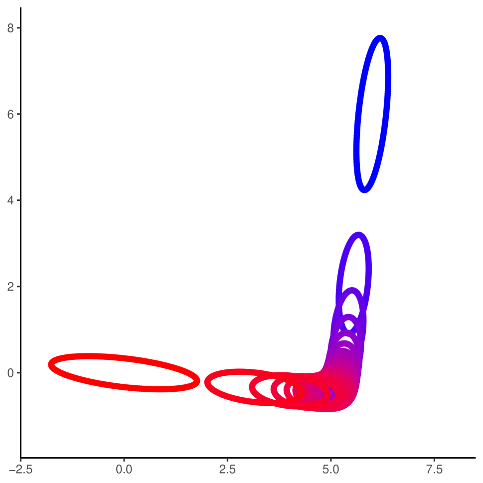
(a)

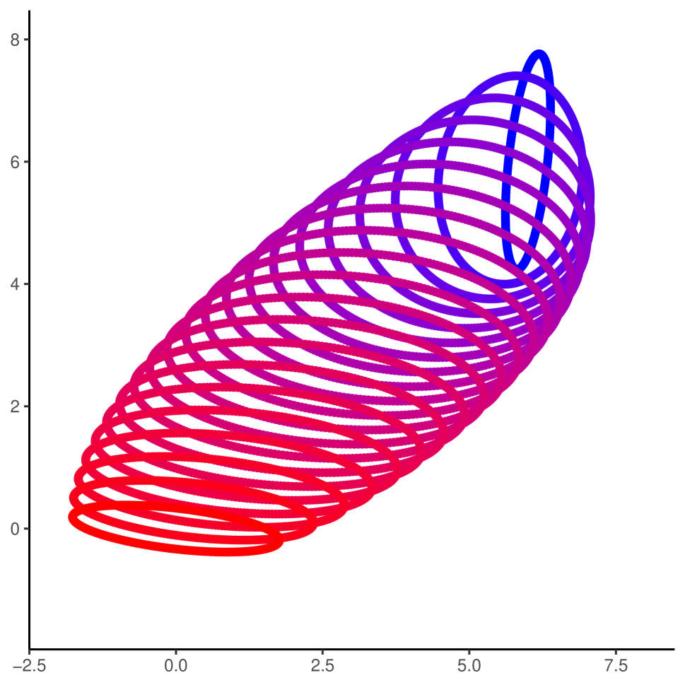
(b)

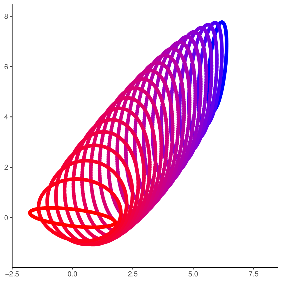
(c)

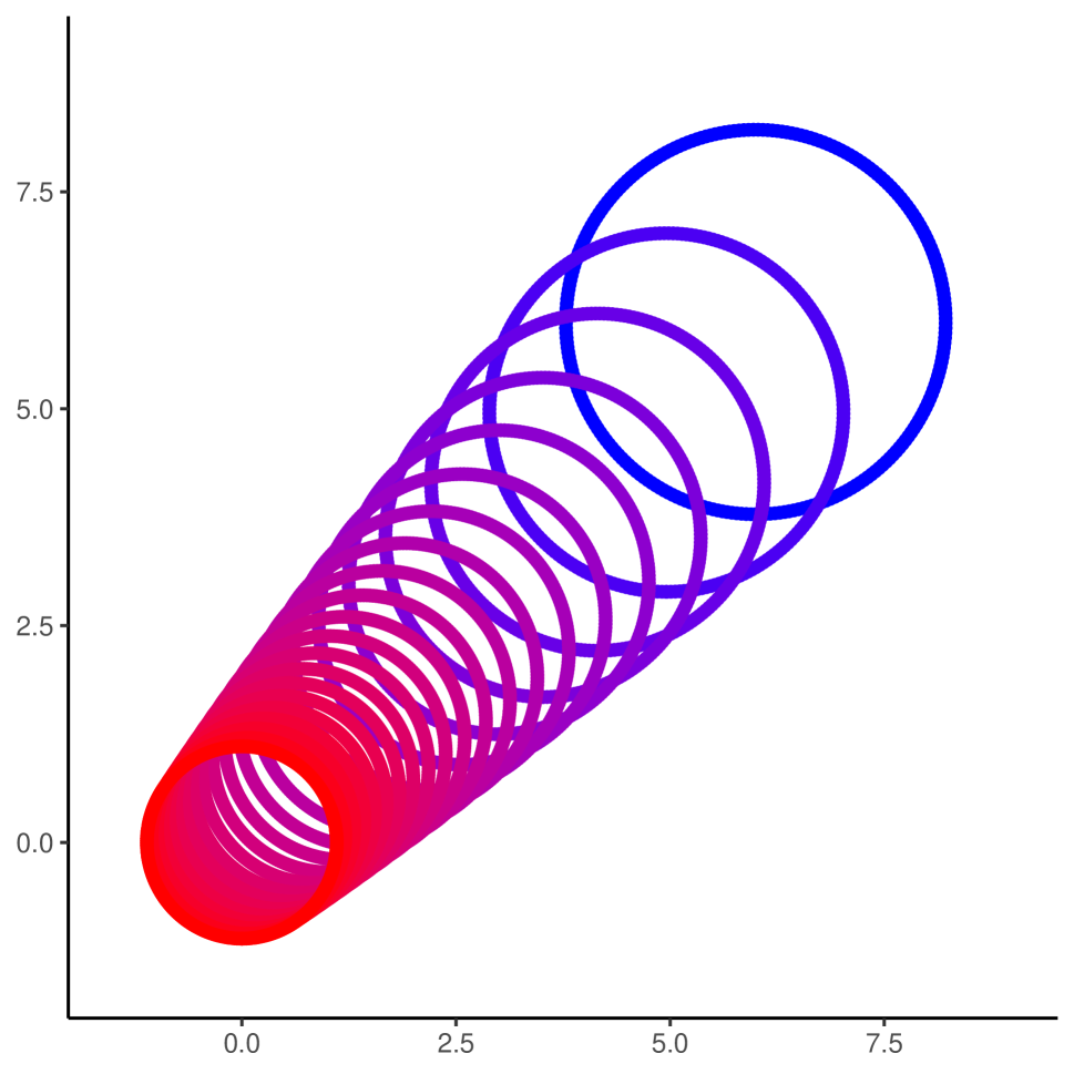
(d)

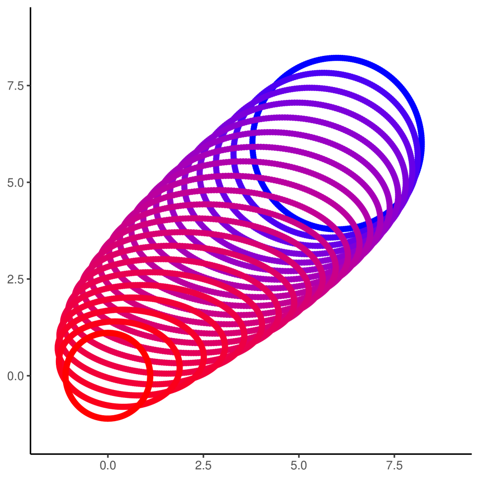
(e)

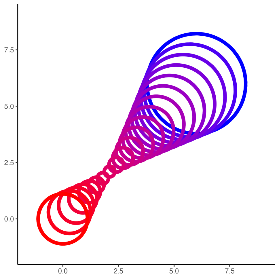
(f)

Figure 1: Subfigures 1(a) and 1(d) depict two examples of the generative distribution of a two-feature Gaussian mixed membership model as specified in Heller et al. (2008). Subfigures 1(b) and 1(c) show two examples of the generative distribution of our proposed mixed membership model with the same mean vectors and covariance matrices as the clusters in Subfigure 1(a), but with varying cross-covariance matrices. Similarly, the generative distributions of Subfigures 1(e) and 1(f) were constructed with the same mean vectors and covariance matrices as the clusters in Subfigure 1(d), but with varying cross-covariance matrices.

In this context, the latent membership scores $Z_{ik}$ can be interpreted, arguably more naturally, as the $i^{th}$ observation’s proportion of membership to the $k^{th}$ feature. Furthermore, denoting with $\boldsymbol{\mathcal{C}}$ the collection of covariance and cross-covariance matrices, we obtain a sampling model defined in terms of the original means and covariances, s.t.

$$\mathbf{y}_{i}\mid\mathbf{z}_{i},\boldsymbol{\nu}_{(1:K)},\boldsymbol{\mathcal{C}}\sim\mathcal{N}\left(\sum_{k=1}^{K}Z_{ik}\boldsymbol{\nu}_{k},\sum_{k=1}^{K}Z_{ik}^{2}\mathbf{C}_{k}+\sum_{k=1}^{K}\sum_{k\neq k^{\prime}}Z_{ik}Z_{ik^{\prime}}\mathbf{C}^{(k,k^{\prime})}\right).$$ (7)

While the random variables $\mathbf{f}_{k}$ could be assumed independent, the inclusion of cross-covariance components allows for greater expressivity and flexibility of the subsequent sampling model. A comparative visualization of the representation offered in Equation (4) versus the model proposed in Equation (7), including the effects of cross-covariance components can be seen in Figure 1. Subfigures 1(a) and 1(d) visualize the distribution of data generated from the Gaussian mixed membership model proposed by Heller et al. (2008). Both scenarios have the same cluster-specific means; however, they have different covariances associated with each cluster. We note that when the major axes of concentration for each cluster are close to orthogonal (Subfigure 1(a)), the generated data appear to lie on a manifold. Alternatively, Subfigures 1(b) and 1(c) show data generated from the proposed mixed membership model. In these two scenarios, each feature has the same mean and covariance as in Subfigure 1(a), but with varying cross-covariance matrices. Even in less extreme settings, such as when component mixtures are spherical (Subfigure 1(d)), our model generalizes sampling expressivity through the introduction of cross-covariance components (Subfigures 1(e) and 1(f)).

From this simple visualization, it is evident that the mixed membership model specified by Equation (4) may lead to mean structures that are hard to interpret, especially in higher dimensions. This interpretability challenge is largely due to the individual feature covariances appearing in the mean term in Equation (4). In contrast, the mean structure in our model is a simple convex combination of individual feature means, where the weighting is directly determined by the membership proportions. More details on our analysis of alternative mixed membership representations are offered in Section 4.

However, increased representational flexibility comes at the cost of an increased dimensional parameter space. Therefore, a concise representation of the covariance structure is needed in order to ensure scalability and regularizability in estimation. In particular, if we were to implement a naïve characterization of the covariance structure, we would need $\mathcal{O}(K^{2}P^{2})$ parameters just to represent the covariance structure, which does not scale well as we increase the dimension of the data ($P$) or the number of clusters ($K$). Instead, we will use a joint decomposition of the $K$ features described in Section 2.2, which will allow us to represent the covariance structure with $\mathcal{O}(KPM)$ parameters, where $M$ is a user-determined variable that controls the accuracy of our representation of the covariance structure. Once we have a concise representation of our $K$ features, we will fully specify a Bayesian version of our proposed mixed membership model in Section 2.3.

2.2 Joint Feature Decomposition

In this section, we construct a joint representation of the $K$ features based on a multivariate eigendecomposition. This joint representation allows for a scalable representation of the underlying high-dimensional covariance structure.

Let $\mathbf{F}=\left[\mathbf{f}_{1},\dots,\mathbf{f}_{K}\right]\in\mathbb{R}^{P\times K},$ be a random matrix that stacks the $K$ latent Gaussian features. We define the corresponding mean matrix, $\boldsymbol{\mu}=\left[\boldsymbol{\nu}_{1},\dots,\boldsymbol{\nu}_{K}\right]$, where $\boldsymbol{\nu}_{k}$ is the mean corresponding to the $k^{th}$ feature. Let $\mathbf{C}^{(k,k^{\prime})}=\text{Cov}\left(\mathbf{f}_{k},\mathbf{f}_{k^{\prime}}\right)$ for $1\leq k,k^{\prime}\leq K$. By vectorizing the matrix $\mathbf{F}$, we obtain

$$\text{Cov}(\text{vec}(\mathbf{F}))=\boldsymbol{\Sigma}=\begin{bmatrix}\mathbf{C}^{(1,1)}&\dots&\mathbf{C}^{(1,K)}\\ \vdots&\ddots&\vdots\\ \mathbf{C}^{(K,1)}&\dots&\mathbf{C}^{(K,K)}\end{bmatrix}.$$ (8)

Since $\boldsymbol{\Sigma}$ is a positive semi-definite matrix, we know that there exists a set of eigenvalues, $\lambda_{1}\geq\lambda_{2},\geq\dots\geq\lambda_{KP}\geq 0$, and a set of eigenvectors, $\boldsymbol{\Psi}_{1},\dots,\boldsymbol{\Psi}_{KP}$, such that

$$\boldsymbol{\Sigma}\boldsymbol{\Psi}_{m}=\lambda_{m}\boldsymbol{\Psi}_{m}.$$

Since the $\boldsymbol{\Psi}_{m}$ are eigenvectors, we know that they are orthonormal. We will define a set of parameters $\boldsymbol{\Phi}_{m}$ such that $\boldsymbol{\Phi}_{m}=\sqrt{\lambda_{m}}\boldsymbol{\Psi}_{m}$. Thus, we can see that $\boldsymbol{\Phi}_{m}$ are still mutually orthogonal, but are scaled by the square root of the corresponding eigenvalue. Consider partitioning $\boldsymbol{\Phi}_{m}$ so that

$$\boldsymbol{\Phi}_{m}=\begin{bmatrix}\boldsymbol{\phi}_{1m}\\ \vdots\\ \boldsymbol{\phi}_{Km}\end{bmatrix}.$$

From Equation (8), by using a spectral decomposition on $\boldsymbol{\Sigma}$, we can see that

$$\mathbf{C}^{(k,k^{\prime})}=\sum_{m=1}^{KP}\boldsymbol{\phi}_{km}\boldsymbol{\phi}_{k^{\prime}m}^{\prime}.$$ (9)

Since $\boldsymbol{\Phi}_{m}$ form a basis for $\mathbb{R}^{KP}$, we have that

$$\text{vec}(\mathbf{F})-\text{vec}(\boldsymbol{\mu}) =\mathbf{P}\circ\left(\text{vec}(\mathbf{F})-\text{vec}(\boldsymbol{\mu})\right)$$

$$=\sum_{m=1}^{KP}\lambda_{m}^{-1}\left\langle\text{vec}(\mathbf{F})-\text{vec}(\boldsymbol{\mu}),\boldsymbol{\Phi}_{m}\right\rangle\boldsymbol{\Phi}_{m},$$ (10)

where $\mathbf{P}$ is the projection operator on $\mathbb{R}^{KP}$. Letting $\chi_{m}=\lambda_{m}^{-1}\left\langle\text{vec}(\mathbf{F})-\text{vec}(\boldsymbol{\mu}),\boldsymbol{\Phi}_{m}\right\rangle$, we can see that

$$\mathbb{E}(\chi_{m}) =\lambda_{m}^{-1}\boldsymbol{\Phi}_{m}^{\prime}\mathbb{E}\left(\text{vec}(\mathbf{F})-\text{vec}(\boldsymbol{\mu})\right)=0,$$

$$\text{Var}\left(\chi_{m}\right) =\text{Cov}\left(\lambda_{m}^{-1}\langle\text{vec}(\mathbf{F}),\boldsymbol{\Phi}_{m}\rangle\right)$$

$$=\lambda_{m}^{-2}\boldsymbol{\Phi}_{m}^{\prime}\text{Cov}(\mathbf{F})\boldsymbol{\Phi}_{m}$$

$$=\lambda_{m}^{-2}\boldsymbol{\Phi}_{m}^{\prime}\left(\sum_{j=1}^{KP}\boldsymbol{\Phi}_{j}\boldsymbol{\Phi}_{j}^{\prime}\right)\boldsymbol{\Phi}_{m}=1.$$

Therefore, using the decomposition in Equation (10), we have that

$$\text{vec}(\mathbf{F})=\text{vec}(\boldsymbol{\mu})+\sum_{m=1}^{KP}\chi_{m}\boldsymbol{\Phi}_{m},$$

where $\chi_{m}\sim\mathcal{N}(0,1)$. To reduce the dimension of the model, we often approximate $\mathbf{F}$ by only using the first $M$ scaled eigenvectors, where $M\leq KP$. Using the first $M$ eigencomponents to approximate $\boldsymbol{\Sigma}$ will give us the best rank $M$ approximation of $\boldsymbol{\Sigma}$ as measured by the Frobenius norm (Eckart-Young-Mirsky Theorem (Eckart and Young, 1936)). Thus, for sufficiently large $M$, we have

$$\text{vec}(\mathbf{F})\approx\text{vec}(\boldsymbol{\mu})+\sum_{m=1}^{M}\chi_{m}\boldsymbol{\Phi}_{m}.$$

Equivalently, we can express this in terms of the $K$ partitioned vectors, such that

$$\mathbf{f}_{k}\approx\boldsymbol{\nu}_{k}+\sum_{m=1}^{M}\chi_{m}\boldsymbol{\phi}_{km}.$$ (11)

From Equation (11), we can see that each feature can be represented by a mean component, $\boldsymbol{\nu}_{k}$, and deviations from the mean controlled by the eigenstructure of the covariance structure of our model, $\boldsymbol{\phi}_{km}$. In this context, the hyperparameter $M$ is defined by the user and controls the approximation accuracy of the covariance structure. If $M=KP$, we are able to recover the true covariance structure. However, in most applications, a relatively small $M$, allows for a good fit to large models, while still ensuring relatively good approximations to the true covariance structure. In the following section, we discuss Bayesian estimation and adopt a regularization approach to select the effective dimension of $M$.

2.3 Sampling Model and Prior Distributions

In this section we combine the convolutional representation of mixed membership introduced in Section 2.1, with the multivariate eigen-approximation of Section 2.2 to define a probability model of mixed membership amenable to formal Bayesian analysis. Using our approximation in Equation (11), we let $\boldsymbol{\Theta}$ be the full collection of model parameters and define the following sampling model:

$$\mathbf{y}_{i}\mid\boldsymbol{\Theta}\sim\mathcal{N}\left\{\sum_{k=1}^{K}Z_{ik}\left(\boldsymbol{\nu}_{k}+\sum_{m=1}^{M}\chi_{im}\boldsymbol{\phi}_{km}\right),\;\sigma^{2}\mathbf{I}_{P}\right\},$$ (12)

where we assume $\chi_{im}\sim_{iid}\mathcal{N}(0,1)$, $(i=1,2,\ldots,N;\;m=1,2,\ldots,M)$. Marginally, integrating out $\chi_{im}$, we recover an approximation to the model in (7):

$$\mathbf{y}_{i}\mid\boldsymbol{\Theta}_{-\chi}\sim\mathcal{N}\left\{\sum_{k=1}^{K}Z_{ik}\boldsymbol{\nu}_{k},\;\sum_{k=1}^{K}\sum_{k^{\prime}=1}^{K}Z_{ik}Z_{ik^{\prime}}\left(\sum_{m=1}^{M}\boldsymbol{\phi}_{km}\boldsymbol{\phi}_{k^{\prime}m}^{\prime}\right)+\sigma^{2}\mathbf{I}_{P}\right\},$$ (13)

where $\boldsymbol{\Theta}_{-\chi}$ denotes the full collection of model parameters excluding the $\chi_{im}$ parameters. Using Equation (9), we can see that the covariance in Equation (13) is a weighted sum of the individual feature covariances and the cross-covariances between the features, with an additional diagonal matrix to capture any residual noise. Similarly, the mean is a weighted sum of the individual feature means. Thus, the model in Equation (13) is what we would expect from a traditional additive model; however, we only need $\mathcal{O}(KPM)$ parameters to estimate the covariance structure. Selecting the number of eigencomponents, $M$, allows one to balance computational cost and model flexibility.

From our derivations in Section 2.2, we know that $\boldsymbol{\Phi}_{k}$ parameters are often assumed to be orthogonal. While aiding likelihood identifiability of the $\boldsymbol{\Phi}$ parameters, this constraint would require posterior simulation on a non-compact Stiefel manifold, which would be computationally challenging, and negatively affect mixing of algorithms using Markov chain Monte Carlo (MCMC) simulations. Section 2.4 shows that we can sample in an unconstrained space while still maintaining many of the desired theoretical properties of our model. Although the $\boldsymbol{\Phi}$ parameters can no longer be interpreted as scaled eigenvectors, posterior samples of the eigenpairs can still be obtained through the posterior samples of the covariance matrix $\boldsymbol{\Sigma}$ in Equation (8).

Furthermore, the eigen-representation of our model in Equation (13), allows for adaptive regularization through shrinkage priors. Specifically, we know that the $\boldsymbol{\phi}_{km}$ should shrink in magnitude as they are scaled by the corresponding eigenvalues. Thus, we leverage the multiplicative gamma process shrinkage prior proposed by Bhattacharya and Dunson (2011). Letting $\phi_{kpm}$ be the $p^{th}$ element of $\boldsymbol{\phi}_{km}$, we can specify our prior as:

$$\phi_{kpm}|\gamma_{kpm},\tilde{\tau}_{mk}\sim\mathcal{N}\left(0,\gamma_{kpm}^{-1}\tilde{\tau}_{mk}^{-1}\right),\;\;\;\gamma_{kpm}\sim\Gamma\left(\nu_{\gamma}/2,\nu_{\gamma}/2\right),\;\;\;\tilde{\tau}_{mk}=\prod_{n=1}^{m}\delta_{nk},$$

$$\delta_{1k}|a_{1k}\sim\Gamma(a_{1k},1),\;\;\;\delta_{jk}|a_{2k}\sim\Gamma(a_{2k},1),\;\;\;a_{1k}\sim\Gamma(\alpha_{1},\beta_{1}),\;\;\;a_{2k}\sim\Gamma(\alpha_{2},\beta_{2}),$$

where $1\leq k\leq K$, $1\leq p\leq P$, $1\leq m\leq M$, and $2\leq j\leq M$ and the gamma distribution is specified by the shape and rate parameters. Since the $\boldsymbol{\Phi}$ parameters can be thought of as eigenvectors scaled by the square root of their corresponding eigenvalues, we would like a prior that promotes shrinkage as $m$ increases. By setting $\alpha_{2}>\beta_{2}$, we have $\mathbb{E}(\delta_{jk})>1$, which will promote shrinkage in $\boldsymbol{\Phi}_{i}$ as $m$ increases. Although we utilize the multiplicative gamma process shrinkage prior (Bhattacharya and Dunson, 2011), alternative methods for regularized inference in factor models (Schiavon et al., 2022; Matuk et al., 2022) can be used to obtain the desired regularized inference.

The model is completed through a conjugate prior for the mean parameters, s.t.

$$\boldsymbol{\nu}_{k}|\tau_{k}\sim\mathcal{N}\left(\mathbf{0}_{P},\tau_{k}\mathbf{I}_{P}\right)\;\;\text{and}\;\;\tau_{k}\sim IG(\alpha,\beta),$$

and, following Heller et al. (2008) and Ghahramani et al. (2014), we assume that

$$\mathbf{z}_{i}|\boldsymbol{\pi},\alpha_{3}\sim Dir(\alpha_{3}\boldsymbol{\pi}),\;\;\;\boldsymbol{\pi}\sim Dir(\mathbf{c}),\;\;\;\alpha_{3}\sim exp(b),$$

for $i=1,\dots,N$. The parameter $\boldsymbol{\pi}$ mainly controls where the prior probability is centered for the allocation parameters. In practice, we often assume that all features are equally likely to be present in the data, and set $\mathbf{c}=\mathbf{1}_{K}$, corresponding to a uniform prior. The concentration of the prior probability on the allocation parameters is controlled by $\alpha_{3}$. In practice, we set $b=10$, which puts slightly higher prior probability that the allocation parameters are close to the vertices of the simplex. In practice, we found that our model was not sensitive to the choice of $\mathbf{c}$ and $b$. Lastly, we assume that $\sigma^{2}\sim IG(\alpha_{0},\beta_{0})$.

2.4 Identifiability and Posterior Consistency

Mixed membership models are subject to non-identifiability problems similar to the ones affecting finite mixture models. As in finite mixture models, a common source of non-identifiability in mixed membership models is what is commonly known as the label switching problem. To solve this problem, we leverage the work of Stephens (2000) and implement relabelling algorithms to post-process the posterior samples after running MCMC simulations.

A second form of non-identifiability stems from the additional flexibility of the allocation parameters, namely that $Z_{ik}\in(0,1)$ rather than just being a binary variable like in a finite mixture model. Consider a two-feature model, where $\boldsymbol{\Theta}_{0}$ denotes the set of “true” parameters (i.e. $(Z_{ik})_{0}$ denotes the true value of $Z_{ik}$). Let $Z_{i1}^{*}=\frac{1}{3}(Z_{i1})_{0}$ and $Z_{i2}^{*}=(Z_{i2})_{0}+\frac{2}{3}(Z_{i1})_{0}$ (transformation preserves the constraint that $Z_{i1}^{*}+Z_{i2}^{*}=1$). If we let $\boldsymbol{\nu}_{1}^{*}=3(\boldsymbol{\nu}_{1})_{0}-2(\boldsymbol{\nu}_{2})_{0}$, $\boldsymbol{\nu}_{2}^{*}=(\boldsymbol{\nu}_{2})_{0}$, $\boldsymbol{\phi}_{1m}^{*}=3(\boldsymbol{\phi}_{1m})_{0}-2(\boldsymbol{\phi}_{2m})_{0}$, $\boldsymbol{\phi}_{2m}^{*}=(\boldsymbol{\phi}_{2m})_{0}$, $\chi_{im}^{*}=(\chi_{im})_{0}$, and $(\sigma^{2})^{*}=\sigma^{2}_{0}$, then from Equation (12), we have $P(\mathbf{y}_{i}|\boldsymbol{\Theta}_{0})=P(\mathbf{y}_{i}|\boldsymbol{\Theta}^{*})$. We will refer to this type of non-identifiability as the rescaling problem. To mitigate the effects of the rescaling problem, we derived the membership rescale algorithm (Algorithm 2 in Section 2.4 of the Supplementary Materials). In a two-feature mixed membership model, the membership rescale algorithm ensures that at least one observation completely lies in each of the features. This assumption that at least one observation completely belongs to each of the features is known as the separability condition (Papadimitriou et al., 1998; McSherry, 2001; Azar et al., 2001; Chen et al., 2022). In the case of the two-feature mixed membership model, this assumption is relatively minor; however, when considering mixed membership models with three or more features, the separability assumption makes relatively strong geometric assumptions. The sufficiently scattered condition (Huang et al., 2016; Jang and Hero, 2019; Chen et al., 2022) makes weaker geometric assumptions, however, it is often more complicated to implement into sampling schemes. In the case when we have more than two features, we leverage the work of Chen et al. (2022), which essentially rescales the allocation parameters so that they cover as much of the unit simplex as possible.

A final source of non-identifiability arises due to the additional flexibility of the allocation parameters. Specifically, when $(\boldsymbol{\nu}_{k^{\prime}})_{0}\propto(\boldsymbol{\phi}_{km})_{0}$ in Equation (12), we can see that the mean vector and covariance matrices are unidentifiable. By assuming the separability condition, we no longer have this non-identifiability issue; however, as stated above, this can be a relatively strong assumption when $K\geq 2$. When assuming weaker assumptions and when $(\boldsymbol{\nu}_{k^{\prime}})_{0}\propto(\boldsymbol{\phi}_{km})_{0}$, then we may not be able to identify the relative magnitude of the parameters. An underestimate of the magnitude of $(\boldsymbol{\phi}_{km})_{0}$ will lead to additional variability in the allocation parameters, leading to wider credible intervals of the $Z_{ik}$ parameters. On the contrary, an overestimate of $(\boldsymbol{\phi}_{km})_{0}$ will lead to smaller credible intervals of the allocation parameters. Since the model is still capturing the variability of the data in this direction, this form of non-identifiability may not be of great concern in practice.

In Section 2.3, we formulated a model where the $\boldsymbol{\Phi}_{m}$ parameters are no longer mutually orthogonal. Therefore, the $\boldsymbol{\Phi}_{m}$ parameters can no longer be interpreted as scaled eigenvectors. However, the relaxation of the orthogonality constraint facilitates easier sampling schemes and the use of “black-box” samplers to obtain samples from the posterior distribution. Relaxation of the orthogonality constraint also tends to lead to better mixing of the Markov chain. Assuming that we can still recover the mean and covariance structure, we can still obtain posterior samples of the eigenvectors by reconstructing posterior draws of the covariance matrix and then calculating the eigenvectors of the sampled covariance matrices. The remaining part of this section will focus on proving that we can recover the mean and covariance structure. However, due to the identifiability issues described earlier in this section, we will be proving weak posterior consistency conditional on knowing the mixing allocation parameters.

Since our main goal is to prove that we can recover the mean and covariance structure, we will be proving weak posterior consistency using the likelihood in Equation (13) (integrating out the $\chi$ parameters). Since $\boldsymbol{\phi}_{km}$ are not identifiable, we will prove posterior consistency with respect to $\boldsymbol{\Sigma}_{kk^{\prime}}:=\sum_{p=1}^{KP}\left(\boldsymbol{\phi}_{kp}\boldsymbol{\phi}^{\prime}_{k^{\prime}p}\right)$. Let $\boldsymbol{\Pi}$ be the prior distribution on $\boldsymbol{\omega}:=\left\{\boldsymbol{\nu}_{1},\dots,\boldsymbol{\nu}_{K},\boldsymbol{\Sigma}_{11},\dots,\boldsymbol{\Sigma}_{1K},\dots,\boldsymbol{\Sigma}_{KK},\sigma^{2}\right\}$. We will denote the set of true parameters as

$$\boldsymbol{\omega}_{0}=\left\{(\boldsymbol{\nu}_{1})_{0},\dots,(\boldsymbol{\nu}_{K})_{0},(\boldsymbol{\Sigma}_{11})_{0},\dots,(\boldsymbol{\Sigma}_{1K})_{0},\dots,(\boldsymbol{\Sigma}_{KK})_{0},\sigma^{2}_{0}\right\}.$$

In order to prove weak posterior consistency, we will have to make the following two assumptions:

Assumption 1

The variables $Z_{ik}$ are known a-priori for $i=1,\dots,N$ and $k=1,\dots,K$.

Assumption 2

The true parameter that models random noise is positive ($\sigma^{2}_{0}>0$).

Under assumptions 1 and 2, we would like to prove that the posterior distribution $\boldsymbol{\Pi}_{N}(.|\mathbf{y}_{1},\dots,\mathbf{y}_{N})$, is weakly consistent at $\boldsymbol{\omega}_{0}\in\boldsymbol{\Omega}$. To do that, we will have to show that there is positive prior probability around the set of true parameters. To do this, we will first define some quantities related to the Kullback–Leibler (KL) divergence. Following the notation of Choi and Schervish (2007), we will define the following quantities:

$$\Lambda_{i}(\boldsymbol{\omega}_{0},\boldsymbol{\omega})=\log\left(\frac{f_{i}(\mathbf{y}_{i};\boldsymbol{\omega}_{0})}{f_{i}(\mathbf{y}_{i};\boldsymbol{\omega})}\right),\;\;K_{i}(\boldsymbol{\omega}_{0},\boldsymbol{\omega})=\mathbb{E}_{\boldsymbol{\omega}_{0}}(\Lambda_{i}(\boldsymbol{\omega}_{0},\boldsymbol{\omega})),\;\;V_{i}(\boldsymbol{\omega}_{0},\boldsymbol{\omega})=\text{Var}_{\boldsymbol{\omega}_{0}}(\Lambda_{i}(\boldsymbol{\omega}_{0},\boldsymbol{\omega})),$$

where $f_{i}(\mathbf{y}_{i};\boldsymbol{\omega}_{0})$ is the likelihood when we have the parameters $\boldsymbol{\omega}_{0}$. To simplify the notation, we will let

$$\boldsymbol{\mu}_{i} =\sum_{k=1}^{K}Z_{ik}\boldsymbol{\nu}_{k},$$

$$\boldsymbol{\Sigma}_{i} =\sum_{k=1}^{K}\sum_{k^{\prime}=1}^{K}Z_{ik}Z_{ik^{\prime}}\left(\sum_{p=1}^{KP}\left(\boldsymbol{\phi}_{kp}\boldsymbol{\phi}^{\prime}_{k^{\prime}p}\right)\right)+\sigma^{2}\mathbf{I}_{P}=\mathbf{U}_{i}^{\prime}\mathbf{D}_{i}\mathbf{U}_{i}+\sigma^{2}\mathbf{I}_{P},$$

where $\mathbf{U}_{i}^{\prime}\mathbf{D}_{i}\mathbf{U}_{i}$ is the spectral decomposition of $\sum_{k=1}^{K}\sum_{k^{\prime}=1}^{K}Z_{ik}Z_{ik^{\prime}}\left(\sum_{p=1}^{KP}\left(\boldsymbol{\phi}_{kp}\boldsymbol{\phi}^{\prime}_{k^{\prime}p}\right)\right)$. Let $\boldsymbol{\Omega}_{\epsilon}(\boldsymbol{\omega}_{0})$ be the set of parameters such that $\boldsymbol{\Omega}_{\epsilon}(\boldsymbol{\omega}_{0}):=\{\boldsymbol{\omega}:K_{i}(\boldsymbol{\omega}_{0},\boldsymbol{\omega})<\epsilon\text{ for all i}\}$. Thus, we have that $\boldsymbol{\Omega}_{\epsilon}(\boldsymbol{\omega}_{0})$ is the set of parameters such that the KL divergence is less than $\epsilon$. We will let $\mathcal{B}(\boldsymbol{\omega}_{0})$ be the set of parameters such that

$$\mathcal{B}(\boldsymbol{\omega}_{0}):=\left\{\boldsymbol{\omega}:\frac{1}{a}\left((d_{il})_{0}+\sigma^{2}_{0}\right)\leq d_{il}+\sigma^{2}\leq a\left((d_{il})_{0}+\sigma^{2}_{0}\right),\|\left(\boldsymbol{\mu}_{i}\right)_{0}-\boldsymbol{\mu}_{i}\|\leq b\right\},$$

for some $a,b\in\mathbb{R}$, where $d_{il}$ is the $l^{th}$ diagonal element of $\mathbf{D}_{i}$.

Lemma 2.1

Let $\mathcal{C}(\boldsymbol{\omega}_{0},\epsilon):=\mathcal{B}(\boldsymbol{\omega}_{0})\cap\boldsymbol{\Omega}_{\epsilon}(\boldsymbol{\omega}_{0})$. Thus, for $\boldsymbol{\omega}_{0}\in\boldsymbol{\Omega}$ and $\epsilon>0$, there exist $a>1$ and $b>0$ such that

1. $\sum_{i=1}^{\infty}\frac{V_{i}(\boldsymbol{\omega}_{0},\boldsymbol{\omega})}{i^{2}}<\infty$, for any $\boldsymbol{\omega}\in\mathcal{C}(\boldsymbol{\omega}_{0},\epsilon)$,

2. $\boldsymbol{\Pi}\left(\boldsymbol{\omega}\in\mathcal{C}(\boldsymbol{\omega}_{0},\epsilon)\right)>0$.

Lemma 2.1 shows us that there are neighborhoods around $\boldsymbol{\omega}_{0}$ that have positive prior probability. Since $\mathbf{y}_{1},\dots,\mathbf{y}_{N}$ are not identically distributed, the first condition of Lemma 2.1 is needed to prove weak posterior consistency.

Lemma 2.2

Under assumptions 1 and 2, the posterior distribution, $\boldsymbol{\Pi}_{N}(.|\mathbf{y}_{1},\dots,\mathbf{y}_{N})$, is weakly consistent at $\boldsymbol{\omega}_{0}\in\boldsymbol{\Omega}$.

Lemma 2.2 states that given the known allocation structure, we are able to recover the mean and covariance structure. Thus, while we cannot directly make inference on the eigenvectors of the covariance structure, we can still recover the covariance structure without enforcing the orthogonality constraint on the $\boldsymbol{\Phi}$ parameters. Although the allocation parameters are usually not known, Lemma 2.1 shows that we have large KL support of the prior in our model specified in Section 2.3. Thus, without enforcing orthogonality constraints on the $\boldsymbol{\Phi}$ and using shrinkage priors on the $\boldsymbol{\Phi}$ parameters to give us the desired regularized estimation, we still have large KL support of the prior; supporting that the modeling decisions of the mean and covariance structures are not restrictive. Due to the complex identifiability problems discussed earlier in this section, it remains elusive to establish weak posterior consistency when $\mathbf{z}_{i}$ are unknown. Although the allocation parameters are usually not known, the empirical evidence in Section 3.1 shows that the mean and covariance structures converge as we obtain more information.

3 Simulations and Case Studies

We conducted two simulation studies to explore the empirical performance of our model and two case studies to illustrate the application of mixed membership models to substantive scientific applications in functional brain imaging and cancer genomics. The first simulation study in Section 3.1 explores the empirical convergence of our model with simulated data. We then look at how information criteria can aid in choosing the number of features in Section 3.2. In Section 3.3, we look at using a mixed membership model to model electroencephalography (EEG) signals in children with Autism spectrum disorder (ASD) and typically developing (TD) children. Lastly, in Section 3.4, we look at how a mixed membership model can be used to classify different breast cancer subtypes using targeted gene expression data.

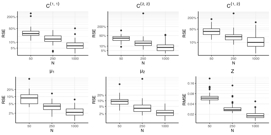
Figure 2: The relative squared error (RSE) for the mean and covariance structure evaluated under various sample sizes. To evaluate the recovery of the allocation parameters, we used the root mean squared error (RMSE).

3.1 Simulation Study 1: Operating Characteristics under Increasing Sample Size

This simulation study focuses on how well we can recover the mean, covariance, and allocation structures under different sample sizes. In this simulation study, we will specifically look at the case when we have 50, 250, and 1000 observations. For each of the three different sample sizes, we generated 50 different datasets with observations $\mathbf{y}_{i}\in\mathbb{R}^{10}$. The data were generated from a two-feature model with $M=4$. More information on how the simulation study was conducted can be found in Section 3.1 of the Supplementary Materials.

To measure how well we can recover the mean vector, covariance matrices, and cross-covariance matrices, we will use the relative squared error (RSE). The RSE is defined as

$$\text{RSE}=\frac{\|f-\hat{f}\|_{2}}{\|f\|_{2}}\times 100\%,$$

where $\|\cdot\|_{2}$ is the Euclidean norm if $f$ is a vector and the Frobenius norm if $f$ is a matrix. In this simulation study, we will use the posterior median as our estimate, $\hat{f}$. To measure how well we can recover the allocation parameters, we will use the root mean squared error (RMSE).

From Figure 2, we can see that our recovery of the mean and covariance structure improves as we obtain more data. While the RSE was relatively large in the simulations when $N=50$, the credible intervals were also significantly wider to account for the uncertainty in the estimate. Specifically, the average credible interval width for the mean vectors when 50 observations were observed was roughly 4.8 times wider than the average credible interval width for the mean vectors when 1000 observations were observed. Overall, this simulation study provides empirical support that the mean and covariance structure converges to the true parameters, even when the allocation parameters are unknown.

3.2 Simulation Study 2: Information Criteria for the Number of Latent Features

In the finite mixed membership setting, inference and interpretation depend on the chosen number of features. To aid in this choice, practitioners often use information criteria (IC) to employ a data-driven approach for the selection of the number of clusters or features for their model. In this section, we study how IC such as AIC (Akaike, 1974), BIC (Schwarz, 1978), and DIC (Celeux et al., 2006; Spiegelhalter et al., 2002) perform in choosing the optimal number of mixtures. In this section, we will also observe how heuristics such as the “elbow-method” perform in choosing the optimal number of clusters.

To evaluate the performance of the IC, we simulated 50 different data sets, where the true number of features was 3. For each data set, four mixed membership models were fit using a varying number of features ($K=2,3,4,$ and $5$). Once the models were fit, we calculated the BIC, AIC, and DIC for each of the models and evaluated the performance of these IC. The definitions of the IC used in this section, as well as detailed information on how the simulation study was conducted, can be found in Section 3.2 of the Supplementary Materials.

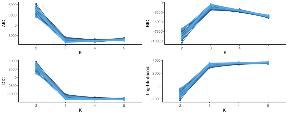
Figure 3: Information Criteria evaluated on our proposed Bayesian mixed membership model for $K=2,3,4,$ and $5$. Information criteria were evaluated on 50 different data sets simulated from a three-feature model.

From Figure 3, we note that the BIC exhibited the most reliable performance, selecting the true number of features all 50 times. Since AIC does not penalize excess parameters as much as BIC, we can see that AIC sometimes selected a model with 4 features over a model with 3 features. Overall, the AIC selected the true number of features only 23 times out of the 50 different datasets and selected a model with four features in 27 of the 50 datasets. In this setting, the DIC was shown to be the least reliable IC, selecting a model with four or more features all 50 times. These results seem to support previous findings that AIC and DIC tend to overestimate the number of features in a model (Frühwirth-Schnatter, 2006; Meyer, 2014). On the contrary, BIC has been shown to be asymptotically consistent for i.i.d. observations from exponential families (Kass and Raftery, 1995) and asymptotically consistent for estimating the number of clusters in Gaussian finite mixture models (Keribin, 2000). From Figure 3, we can see that all the IC considered in this section were unlikely to underestimate the number of features in our model, supporting the results of Leroux (1992) who showed that AIC and BIC asymptotically do not underestimate the number of components in mixture models.

As discussed in Marco et al. (2022), the average log-likelihood can aid in the selection of the optimal number of features in mixed membership models. From Figure 3, we can see that there is a distinct “elbow” at $K=3$. Using the elbow method, we would correctly identify the correct number of features all 50 times. Although BIC had the same performance as the “elbow-method”, we can see from Figure 3 that BIC sometimes returned very similar values for three-feature and four-feature models, suggesting that there may be a slight tendency to choose an overfit model. However, the results from the “elbow-method” were more definitive, as there is a distinct elbow at $K=3$ for each dataset. However, the “elbow-method” cannot be used when deciding between two-feature and three-feature models. Therefore, we recommend using BIC in conjunction with the “elbow-method” to select the optimal number of features for our proposed model.

3.3 A Case Study on Functional Brain Imaging through EEG

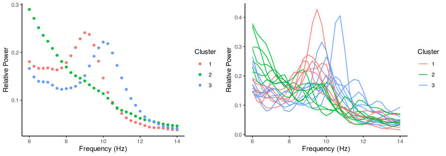
Figure 4: (Left Panel) Recovered means from fitting a $k$-means model with 3 clusters. (Right Panel) Data from the T8 electrode of 20 individuals with varying clinical diagnosis (TD vs. ASD), colored by the estimated cluster membership.

Autism spectrum disorder (ASD) is a disorder characterized by social communication deficits and/or unusual sensory-motor behaviors (Lord et al., 2018; Edition, 2013). Although once a more narrowly defined disorder, autism is now seen as a wide spectrum of symptoms, ranging from very mild symptoms to severe symptoms that can require lifelong care. In this case study, we analyze electroencephalogram (EEG) data collected in 39 typically developing (TD) children and 58 children diagnosed with ASD, between the ages of 2 and 12 years old (Dickinson et al., 2018). EEG data in the present analysis are considered spontaneous because they reflect intrinsic functional brain dynamics under task-free conditions. EEG data were recorded for two minutes using a 128-channel HydroCel Geodesic Sensory net. During the recording, the children were seated in front of a computer monitor that displayed floating bubbles, a commonly used approach to collect resting EEG data in developmental populations (Dawson et al., 1995; Stroganova et al., 1999; Tierney et al., 2012; McEvoy et al., 2015). The signals from the sensors were filtered to remove signals outside of the 0.1 to 100 Hz band range and then interpolated to match the international 10-20 system 25 channel montage. A fast Fourier transform was then applied to the data to transform the data into the frequency domain. In this analysis, we consider the relative power in the frequency domain, which means that each function is scaled to integrate to 1. Visualizations of the data, as well as the results of a $k$-means analysis (Lloyd, 1982), can be seen in Figure 4.

When neuroscientists evaluate resting-state EEG data, one area of interest is the location of a single prominent peak in the spectral density located in the alpha band of frequencies (6-14 Hz), called the peak alpha frequency (PAF). The emergence of this peak has been shown to be a biomarker of neural development in typically developing children (Rodríguez-Martínez et al., 2017). A clear alpha peak gradually emerges during the first year of life in typically developing children and increases in frequency over childhood before reaching stability in adolescence/early adulthood (Rodríguez-Martínez et al., 2017; Scheffler et al., 2019). On the other hand, both the emergence of peak alpha frequency and developmental frequency shifts have been shown to be atypical in children diagnosed with ASD. More specifically, children are less likely to display a clear alpha peak than age-matched peers, and do not show the same age-related increase that is well documented in typical children (Scheffler et al., 2019).

In this case study, we performed a multivariate analysis of the EEG analysis using the average power of the 25 electrodes at 33 frequencies of interest in the alpha frequency band (from 6 Hz to 14 Hz with step sizes of 0.25 Hz). Using the information criteria discussed in Section 3.2, we found that a mixed membership model with 2 features seemed to be optimal. Thus, we fit a two-feature mixed membership model ($K=2$) with five eigenvectors ($M=5$), and ran our chain for 500,000 iterations. To save computational resources, the Markov chain was thinned, saving every $10^{th}$ iteration.

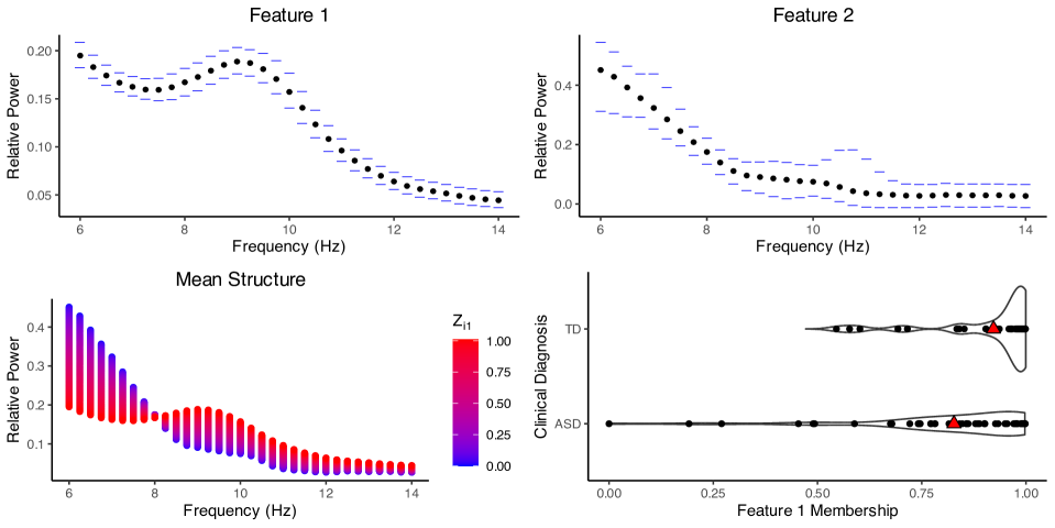
Figure 5: (Top Panels) Posterior median estimates of the mean vectors of the features, with corresponding 95% credible intervals. (Bottom Left Panel) Posterior median estimates of the mean structure conditional on feature membership. (Bottom Right Panel) Posterior median estimates of the membership to the first feature, stratified by clinical cohort. The red triangles represent the mean membership to the first feature.

From Figure 5, we can see that the first functional feature can be interpreted as a distinct alpha peak. On the other hand, the second feature can be interpreted as a $1/f$ trend, or pink noise. These two features help to differentiate between periodic (alpha waves) and aperiodic ($1/f$ trend) neural activity patterns, which coexist in the EEG spectra. Loading heavily on feature 2 suggests that the 1/f trend is the most prominent in an individual’s EEG recording, suggesting that a clear alpha peak has not yet emerged. From Figure 5, we can see that typically developing children seem to heavily load on the first feature, representing individuals with a distinct alpha peak. On the other hand, children with ASD seem to have relatively high heterogeneity in their loadings. We can see that on average children with ASD tend to have a more attenuated alpha peak (more loading on feature 2), with some individuals having no discernible alpha peak at all. These results closely match the results obtained by Marco et al. (2022), who used a functional mixed membership model to model the spectral density as a random function.

Given that the presence and/or emergence of an alpha peak is a developmental biomarker, objectively quantifying the presence of a peak is important. By allowing individuals to partially belong to both features, we are able to objectively quantify the presence of a clear alpha peak over and above $1/f$ aperiodic patterns. This approach offers a novel way to quantify the progression of alpha peak emergence in individuals where the peak has not yet reached maturity. Visualizations of the recovered covariance structure can be found in Section 3.3 of the Supplementary Materials.

Figures 4 and 5 clearly depict the differences between traditional clustering models, like a $k$-means model (Lloyd, 1982), and our proposed mixed membership model. Information criteria determined that 3 clusters were the optimal number of clusters for a $k$-means analysis, illustrating how the increased flexibility of mixed membership models can potentially represent data using fewer clusters than traditional clustering. In the $k$-means analysis, the first and third clusters can be interpreted as distinct alpha peaks, while the second cluster can be interpreted as primarily $1/f$ aperiodic patterns. Although the cluster means found in the $k$-means analysis are relatively interpretable, we lose the ability to quantify the ratio of periodic signals to aperiodic signals, which is of significant scientific interest. From a modeling standpoint, traditional clustering models assume that each observation comes from one of the three clusters, meaning that children who have a developing alpha peak are not represented by any of the three clusters. Alternatively, the mixed membership model assumes that each observation can be represented by a continuous mixture of periodic and aperiodic neural activity patterns, leading to a more natural sampling model that is supported by previous scientific literature.

3.4 A Case Study on Molecular Subtypes in Breast Cancer

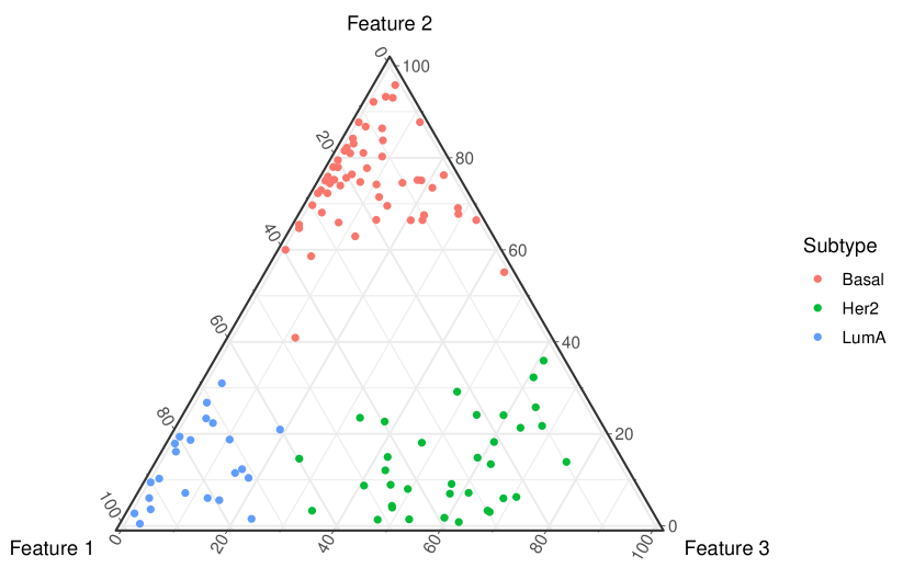
Figure 6: Estimated feature membership stratified by cancer subtype.

As of 2015, breast cancer is the $29^{th}$ leading cause of death in the world, with an estimated 534,000 deaths per year (Wang et al., 2016). Although there has been a significant increase in the number of deaths between 2005 and 2015 (21.3%), the age-adjusted death rate has decreased by 6.8% mainly due to our increased understanding of how to treat breast cancer. In the last two decades, five molecular subtypes of breast cancer have been discovered; each with a different prognosis, risk factors, and treatment sensitivity (Prat et al., 2015). Parker et al. (2009) discovered that the cancer subtype can be accurately classified using centroid-based prediction methods using gene expression data from 50 genes (known as PAM50). Although there are five commonly accepted subtypes, newer studies have found up to ten molecular subtypes (Curtis et al., 2012), while others theorize that multiple cancer subtypes can coexist within a tumor (Yeo and Guan, 2017). Although the number of subgroups and even the definition of the subgroups have evolved over the years (Orrantia-Borunda et al., 2022), the main purpose of creating these subgroups is to explain the inter- and intratumoral heterogeneity leading to differential treatments to elicit the best response in patients (Yeo and Guan, 2017). In this case study, we propose modeling heterogeneity through a mixed membership model, which allows for a more expressive model while building upon the well-accepted idea of five molecular subtypes.

Following Xu et al. (2016), we will use the PAM50 dataset to fit a mixed membership model on patients with LumA, Basal, and Her2 cancer subtypes. When restricting the PAM50 dataset to these three cancer subtypes, we have 115 patients with breast cancer ($N=115$), and 50 genes of interest ($P=50$). To build on the idea of the three well-accepted cancer subtypes, we fit a three-feature mixed membership model ($K=3$) with four eigenvectors to approximate the covariance structure ($M=4$).

From Figure 6, we can see that each feature corresponds to a specific breast cancer subtype. While the data are still separable by cancer subtype, we can see that there is considerable overlap between features 1 and 3 for some of the patients who were classified with the Her2 cancer subtype. The added flexibility of a mixed membership model is crucial as physicians can offer more personalized treatment plans for each patient. Since each cancer subtype has particular risk factors and treatment sensitivity, physicians who have patients that load heavily on two or more features will be aware that they should be monitoring all risk factors in the corresponding features. Treatment plans can also be customized to account for the treatment sensitivity of two or more cancer subtypes.

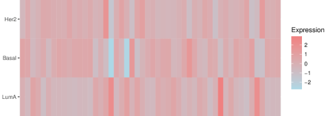
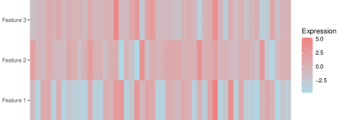
Figure 7: Cluster centroids for the model constructed by Parker et al. (2009)(left) and the feature means for our mixed membership model (right).

From Figure 7, we can see that there is more heterogeneity in the mean structure of our model than in the cluster centroids found in Parker et al. (2009). Conceptually, these mean structures represent two different ideas. In centroid-based clustering, the data is assumed to belong to only one of the cancer subtypes. Therefore, the mean structure in the centroid-based clustering model represents the average gene expression values for an individual belonging to that cluster. On the other hand, our model assumes that each individual can simultaneously belong to multiple cancer subtype groups. Therefore, the mean for a particular feature represents the average gene expression values for an individual that only belongs to that feature. Thus, the mean structure for the mixed membership model is more heterogeneous because they represent the “extreme” cases, or cases that are the most dissimilar from the other cancer subtypes. Overall, the added flexibility offered by our proposed mixed membership model allows us to maintain the well-accepted subgroups of LumA, Basal, and Her2, while having a more expressive model that explains more heterogeneity than comparable centroid-based models. The ability to explain more heterogeneity is advantageous from a clinical perspective as more personalized treatment plans can be constructed. Moreover, the use of mixed membership model over adding more clusters to a centroid-based model is advantageous as it will be more parsimonious. Lastly, the idea that multiple cancer subtypes can exist within a tumor (Yeo and Guan, 2017) is closely related to our model; since the mixed membership model in this section suggests that each individual can be represented as a continuous mixture of the three cancer subtypes modeled in this section. Visualizations of the correlation structure of features can be found in Section 3.4 of the Supplementary Materials.

4 Discussion

This manuscript introduces a flexible, yet scalable mixed membership model for continuous multivariate data. Mixed membership models, sometimes referred to as partial membership models or admixture models, can be thought of as a generalization of clustering, where each observation can partially belong to multiple clusters. In Section 2, we derive our mixed membership model by extending the framework of finite mixture models. To have a scalable framework, we use a spectral decomposition of the $K$ features, leveraging the multiplicative gamma shrinkage prior to ensure that the scaled eigenvectors are stochastically shrunk. To facilitate the use of simple sampling methods, we removed the constraint that the scaled eigenvectors, $\boldsymbol{\Phi}_{m}$, had to be mutually orthogonal. Within this context, we proved that the model had conditional weak posterior consistency of our mean and covariance structures, allowing us to facilitate relatively simple sampling schemes. Compared to previous work on mixed membership models, our proposed model has an easily interpretable mean and covariance structure, allowing practitioners to easily and effectively communicate their findings from the model.

For the case of continuous data, the mixed membership model representation proposed by Heller et al. (2008) and discussed by (Ghahramani et al., 2014; Gruhl and Erosheva, 2014) is seemingly natural and generally applicable to data assumed to be sampled from a multivariate exponential family of distributions. We note that for the case of Normally distributed mixture components, this framework may prove to be too rigid to model more complex datasets. The Subfigures 1(a) and 1(d) contain visualizations of the distribution of data generated from the Gaussian mixed membership model proposed by Heller et al. (2008). Both scenarios have the same cluster-specific means; however, they have different covariances associated with each cluster. In this setting, the generated data follow the direction associated with the eigenvectors of the pure mixture covariance matrices, which can lead to unwieldy implied trajectories for plausible data realizations, e.g. data lying on a manifold (Subfigure 1(a)). Alternatively, Subfigures 1(b) and 1(c) show the data generated from our proposed mixed membership model. In these two scenarios, each feature has the same mean and covariance as in Subfigure 1(a), but they have different cross-covariance matrices. In these cases, we can see a more natural trajectory of the data, where an assumption of a Euclidean metric seems appropriate. In less extreme settings, such as assuming spherical contours for the pure mixture components (Subfigure 1(d)), the representation in Equation (4) still leads to natural trajectories for the generated data, where the variance monotonically grows as the observation moves from the red to the blue cluster. Crucially, the proposed mixed membership model in Equation (7) recovers the model in Equation (4) as a special case, by setting the cross-covariance matrix equal to the zero matrix. However, the inclusion of cross-covariance elements can express more flexible sampling scenarios, as shown in Subfigures 1(e) and 1(f). Specifically, in Subfigure 1(e) we show the distribution of data where the symmetric part of the cross-covariance matrix has positive eigenvalues, while 1(f) shows the distribution of data where the symmetric part of the cross-covariance matrix has negative eigenvalues. Overall, the inclusion of explicit cross-covariance elements and the additive nature of our model leads to more natural trajectories of the implied model and an increased expressivity of the implied data generating process.

Mixed membership models for continuous data, as encoded in our representation in Equation (5), are related to latent factor models, as they rely on similar additive structures. Nevertheless, mixed membership models obtain an alternative decomposition of data variation, leading to a different interpretation of the model parameters. An illustration of the differences between Gaussian finite mixture models, factor models, and our proposed mixed membership model can be seen in Figure 8. The principal difference between factor models and mixed membership models being that mixed membership models restrict mixing between latent features to be defined on the standard simplex. As a consequence, the ensuing model defines margins which are not constrained to be elliptically symmetric, as in the case of factor models. An in-depth discussion of how factor analysis compares to mixed membership modeling is provided in Section 4 of the Supplementary Materials.

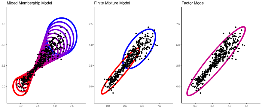
Figure 8: Comparative visualization of the differences between mixed membership models, finite mixture models, and factor models. Each of the models were fit on the same set of data, illustrated by the black dots.

Although flexibility is crucial to ensure that the model fits the data adequately, interpretability of a model is paramount when communicating scientific findings. Under the Gaussian mixed membership model framework described by Heller et al. (2008), each observation is distributed normally, where the natural parameters of the distribution are a convex combination of the natural parameters associated with each cluster. The natural parameter representation can be particularly difficult to work with because the mean structure is influenced by the covariance matrices of each individual cluster, leading to unnatural trajectories as seen in Subfigure 1(a). Although the mean structure can be easily visualized in low dimensions, visualization of the mean structure can be particularly challenging in a high-dimensional model, leading to challenges in communicating the overall scientific findings. In our proposed model, each observation is also normally distributed; however, the mean parameter is simply a convex combination of the individual features’ mean parameters. Similarly, the covariance of each observation can be written as a weighted sum of the covariance and cross-covariance functions of the features. Overall, this simple structure allows practitioners to easily describe the distribution of observations that belong to multiple features while maintaining a relatively flexible model.

From a practitioner’s perspective, the main challenge in fitting a mixed membership model is choosing the number of features ($K$). Similarly to finite mixture models (Frühwirth-Schnatter, 2006), mixed membership models also suffer from non-identifiability problems due to overfitting. Therefore, choosing the correct number of features in a mixed membership model is crucial, as underspecifying the number of features will lead to a model that lacks the required flexibility needed to model the variability of the data, while overspecifying the number of features can lead to a lack of interpretability. As shown in Section 3.2, information criteria and simple heuristics, such as the “elbow” method, can be very informative in choosing the number of features in a mixed membership model. In traditional finite mixture models, Rousseau and Mengersen (2011) and Nguyen (2013) have shown that under certain conditions, an overfit mixture model would have a posterior distribution where only the “true” parameters would have positive weight, and the rest of the parameters would converge to zero. In both manuscripts, they assumed that the parameters were identifiable if we disregard the non-identifiability caused by the label-switching problem. However, as discussed in Section 2.4, the continuous nature of the allocation parameters create multiple non-identifiability problems. These types of non-identifiability problems make applying the results from Rousseau and Mengersen (2011) and Nguyen (2013) non-trivial. An alternative non-parametric approach can be used by leveraging the Indian Buffet Process (Griffiths and Ghahramani, 2011), allowing for an infinite number of potential clusters. However, implementing and conducting inference across changing dimensions is a non-trivial task and still an active area of research. In addition to the number of features, users are also tasked with choosing the number of eigenvectors ($M$) to use in the mixed membership model. The number of eigenvectors controls how accurately we can approximate the covariance structure of the model. If $M=KP$, then we have a fully saturated model, and we can have an exact representation of the covariance structure. In large models, setting $M=KP$ may be computationally intractable, which means that we will have to approximate the covariance structure by using a low-rank approximation of the covariance structure. Thus, the choice of $M$ is a user-defined choice that depends primarily on the computational budget afforded to fit the model.

Due to the added flexibility of mixed membership models in general, we are often faced with multiple modal posterior distributions. Due to the potential multiple-modal nature of the posterior distribution, we implemented tempered transitions (Section 2.3 of the Supplementary Materials) to ensure adequate exploration of the posterior distribution by allowing the chain to traverse areas of low posterior probability. Although tempered transitions theoretically allow you to move between modes of the posterior distribution, they can be computationally expensive and sometimes tricky to tune. To limit the computational burden, we suggest a mixture of tempered transitions and untempered transitions when performing MCMC. To speed up convergence of the Markov chain, we pick an informative starting position for our parameters using the multiple start algorithm (Algorithm 1) described in Section 2.2 of the Supplementary Materials. The added flexibility of the allocation parameters also causes the rescaling problem described in Section 2.4. To make interpretation easier for practitioners, we recommend using the membership rescale algorithm (Algorithm 2) described in Section Section 2.4 of the Supplementary Materials. In the two-feature case, this algorithm ensures that at least one observation belongs entirely to one feature. In the case where we have more than two features, the algorithm can be reformulated as an optimization problem. An R package for our proposed Gaussian mixed membership model is available for download at https://github.com/ndmarco/BayesFMMM.

Acknowledgements
The authors gratefully acknowledge funding from the NIH/NIMH R01MH122428-01 (DS,DT).

References

- Akaike (1974) Akaike, H., 1974. A new look at the statistical model identification. IEEE transactions on automatic control 19, 716–723.
- Alexander et al. (2009) Alexander, D.H., Novembre, J., Lange, K., 2009. Fast model-based estimation of ancestry in unrelated individuals. Genome research 19, 1655–1664.
- Azar et al. (2001) Azar, Y., Fiat, A., Karlin, A., McSherry, F., Saia, J., 2001. Spectral analysis of data, in: Proceedings of the thirty-third annual ACM symposium on Theory of computing, pp. 619–626.
- Bhattacharya and Dunson (2011) Bhattacharya, A., Dunson, D.B., 2011. Sparse bayesian infinite factor models. Biometrika , 291–306.
- Blei et al. (2003) Blei, D., Ng, A., Jordan, M., 2003. Latent Dirichlet allocation. JMLR .
- Broderick et al. (2013) Broderick, T., Pitman, J., Jordan, M., 2013. Feature allocations, probability functions, and paintboxes. Bayesian Analysis 8, 801–836.
- Celeux et al. (2006) Celeux, G., Forbes, F., Robert, C.P., Titterington, D.M., 2006. Deviance information criteria for missing data models. Bayesian analysis 1, 651–673.
- Chen et al. (2022) Chen, Y., He, S., Yang, Y., Liang, F., 2022. Learning topic models: Identifiability and finite-sample analysis. Journal of the American Statistical Association , 1–16.
- Choi and Schervish (2007) Choi, T., Schervish, M.J., 2007. On posterior consistency in nonparametric regression problems. Journal of Multivariate Analysis 98, 1969–1987. doi:https://doi.org/10.1016/j.jmva.2007.01.004.
- Curtis et al. (2012) Curtis, C., Shah, S.P., Chin, S.F., Turashvili, G., Rueda, O.M., Dunning, M.J., Speed, D., Lynch, A.G., Samarajiwa, S., Yuan, Y., et al., 2012. The genomic and transcriptomic architecture of 2,000 breast tumours reveals novel subgroups. Nature 486, 346–352.
- Dawson et al. (1995) Dawson, G., Klinger, L.G., Panagiotides, H., Lewy, A., Castelloe, P., 1995. Subgroups of autistic children based on social behavior display distinct patterns of brain activity. Journal of abnormal child psychology 23, 569–583.
- Dickinson et al. (2018) Dickinson, A., DiStefano, C., Senturk, D., Jeste, S.S., 2018. Peak alpha frequency is a neural marker of cognitive function across the autism spectrum. European Journal of Neuroscience 47, 643–651.
- Eckart and Young (1936) Eckart, C., Young, G., 1936. The approximation of one matrix by another of lower rank. Psychometrika 1, 211–218.
- Edition (2013) Edition, F., 2013. Diagnostic and statistical manual of mental disorders. Am Psychiatric Assoc 21, 591–643.
- Erosheva et al. (2004) Erosheva, E., Fienberg, S., Lafferty, J., 2004. Mixed membership models of scientific publications. PNAS .
- Frühwirth-Schnatter (2006) Frühwirth-Schnatter, S., 2006. Finite mixture and Markov switching models. Springer.
- Galyardt (2014) Galyardt, A., 2014. Interpreting mixed membership: Implications of Erosheva’s representation theorem.. CRC Press. chapter 3.
- Ghahramani et al. (2014) Ghahramani, Z., Mohamed, S., Heller, K., 2014. A Simple and General Exponential Family Framework for Partial Membership and Factor Analysis. CRC Press. chapter 4.
- Griffiths and Ghahramani (2011) Griffiths, T., Ghahramani, Z., 2011. The Indian buffet process: An introduction and review. Journal of Machine Learning Research 12, 1185–1224.
- Gruhl and Erosheva (2014) Gruhl, J., Erosheva, E., 2014. A Tale of Two (Types of) Memberships: Comparing Mixed and Partial Membership with a Continuous Data Example. CRC Press. chapter 2.
- Heller et al. (2008) Heller, K.A., Williamson, S., Ghahramani, Z., 2008. Statistical models for partial membership, in: Proceedings of the 25th International Conference on Machine learning, pp. 392–399.
- Hennig et al. (2015) Hennig, C., Meila, M., Murtagh, F., Rocci, r., 2015. Handbook of Cluster Analysis. CRC Press.
- Hou-Liu and Browne (2022) Hou-Liu, J., Browne, R.P., 2022. Chimeral clustering. Journal of Classification , 1–20.
- Huang et al. (2016) Huang, K., Fu, X., Sidiropoulos, N.D., 2016. Anchor-free correlated topic modeling: Identifiability and algorithm. Advances in Neural Information Processing Systems 29.
- Jang and Hero (2019) Jang, B., Hero, A., 2019. Minimum volume topic modeling, in: The 22nd International Conference on Artificial Intelligence and Statistics, PMLR. pp. 3013–3021.
- Kass and Raftery (1995) Kass, R.E., Raftery, A.E., 1995. Bayes factors. Journal of the american statistical association 90, 773–795.
- Keribin (2000) Keribin, C., 2000. Consistent estimation of the order of mixture models. Sankhyā: The Indian Journal of Statistics, Series A , 49–66.
- Lee et al. (2016) Lee, J., Müller, P., Sengupta, S., Gulukota, K., Ji, Y., 2016. Bayesian inference for intratumour heterogeneity in mutations and copy number variation. Journal of the Royal Statistical Society: Series C (Applied Statistics) 65, 547–563. URL: https://rss.onlinelibrary.wiley.com/doi/abs/10.1111/rssc.12136, doi:https://doi.org/10.1111/rssc.12136, arXiv:https://rss.onlinelibrary.wiley.com/doi/pdf/10.1111/rssc.12136.
- Leroux (1992) Leroux, B.G., 1992. Consistent estimation of a mixing distribution. The Annals of Statistics , 1350–1360.
- Lloyd (1982) Lloyd, S., 1982. Least squares quantization in pcm. IEEE transactions on information theory 28, 129–137.
- Lord et al. (2018) Lord, C., Elsabbagh, M., Baird, G., Veenstra-Vanderweele, J., 2018. Autism spectrum disorder. The Lancet 392, 508–520.
- Marco et al. (2022) Marco, N., Şentürk, D., Jeste, S., DiStefano, C., Dickinson, A., Telesca, D., 2022. Functional mixed membership models. arXiv preprint arXiv:2206.12084 .
- Matuk et al. (2022) Matuk, J., Herring, A.H., Dunson, D.B., 2022. Bayesian functional principal components analysis using relaxed mutually orthogonal processes. arXiv preprint arXiv:2205.12361 .
- McEvoy et al. (2015) McEvoy, K., Hasenstab, K., Senturk, D., Sanders, A., Jeste, S.S., 2015. Physiologic artifacts in resting state oscillations in young children: methodological considerations for noisy data. Brain imaging and behavior 9, 104–114.
- McSherry (2001) McSherry, F., 2001. Spectral partitioning of random graphs, in: Proceedings 42nd IEEE Symposium on Foundations of Computer Science, IEEE. pp. 529–537.
- Meyer (2014) Meyer, R., 2014. Deviance information criterion (dic). Wiley StatsRef: Statistics Reference Online , 1–6.
- Nguyen (2013) Nguyen, X., 2013. Convergence of latent mixing measures in finite and infinite mixture models. The Annals of Statistics 41, 370–400.
- Orrantia-Borunda et al. (2022) Orrantia-Borunda, E., Anchondo-Nuñez, P., Acuña-Aguilar, L.E., Gómez-Valles, F.O., Ramírez-Valdespino, C.A., 2022. Subtypes of breast cancer. Breast Cancer [Internet] .
- Papadimitriou et al. (1998) Papadimitriou, C.H., Tamaki, H., Raghavan, P., Vempala, S., 1998. Latent semantic indexing: A probabilistic analysis, in: Proceedings of the seventeenth ACM SIGACT-SIGMOD-SIGART symposium on Principles of database systems, pp. 159–168.
- Parker et al. (2009) Parker, J.S., Mullins, M., Cheang, M.C., Leung, S., Voduc, D., Vickery, T., Davies, S., Fauron, C., He, X., Hu, Z., et al., 2009. Supervised risk predictor of breast cancer based on intrinsic subtypes. Journal of clinical oncology 27, 1160.
- Prat et al. (2015) Prat, A., Pineda, E., Adamo, B., Galván, P., Fernández, A., Gaba, L., Díez, M., Viladot, M., Arance, A., Muñoz, M., 2015. Clinical implications of the intrinsic molecular subtypes of breast cancer. The Breast 24, S26–S35.
- Pritchard et al. (2000) Pritchard, J.K., Stephens, M., Donnelly, P., 2000. Inference of population structure using multilocus genotype data. Genetics 155, 945–959.
- Rodríguez-Martínez et al. (2017) Rodríguez-Martínez, E., Ruiz-Martínez, F., Paulino, C.B., Gómez, C.M., 2017. Frequency shift in topography of spontaneous brain rhythms from childhood to adulthood. Cognitive neurodynamics 11, 23–33.
- Rousseau and Mengersen (2011) Rousseau, J., Mengersen, K., 2011. Asymptotic behaviour of the posterior distribution in overfitted mixture models. Journal of the Royal Statistical Society: Series B (Statistical Methodology) 73, 689–710.
- Ruspini et al. (2019) Ruspini, E.H., Bezdek, J.C., Keller, J.M., 2019. Fuzzy clustering: A historical perspective. IEEE Computational Intelligence Magazine 14, 45–55.
- Scheffler et al. (2019) Scheffler, A.W., Telesca, D., Sugar, C.A., Jeste, S., Dickinson, A., DiStefano, C., Şentürk, D., 2019. Covariate-adjusted region-referenced generalized functional linear model for eeg data. Statistics in medicine 38, 5587–5602.
- Schiavon et al. (2022) Schiavon, L., Canale, A., Dunson, D.B., 2022. Generalized infinite factorization models. Biometrika 109, 817–835.
- Schwarz (1978) Schwarz, G., 1978. Estimating the dimension of a model. The annals of statistics , 461–464.
- Spiegelhalter et al. (2002) Spiegelhalter, D.J., Best, N.G., Carlin, B.P., Van Der Linde, A., 2002. Bayesian measures of model complexity and fit. Journal of the royal statistical society: Series B (statistical methodology) 64, 583–639.
- Stephens (2000) Stephens, M., 2000. Dealing with label switching in mixture models. Journal of the Royal Statistical Society: Series B (Statistical Methodology) 62, 795–809.
- Stroganova et al. (1999) Stroganova, T.A., Orekhova, E.V., Posikera, I.N., 1999. Eeg alpha rhythm in infants. Clinical neurophysiology 110, 997–1012.
- Tang et al. (2005) Tang, H., Peng, J., Wang, P., Risch, N.J., 2005. Estimation of individual admixture: analytical and study design considerations. Genetic Epidemiology: The Official Publication of the International Genetic Epidemiology Society 28, 289–301.
- Tierney et al. (2012) Tierney, A.L., Gabard-Durnam, L., Vogel-Farley, V., Tager-Flusberg, H., Nelson, C.A., 2012. Developmental trajectories of resting eeg power: an endophenotype of autism spectrum disorder. PloS one 7, e39127.
- Wang et al. (2016) Wang, H., Naghavi, M., Allen, C., Barber, R.M., Bhutta, Z.A., Carter, A., Casey, D.C., Charlson, F.J., Chen, A.Z., Coates, M.M., et al., 2016. Global, regional, and national life expectancy, all-cause mortality, and cause-specific mortality for 249 causes of death, 1980–2015: a systematic analysis for the global burden of disease study 2015. The lancet 388, 1459–1544.
- Xu et al. (2016) Xu, Y., Müller, P., Telesca, D., 2016. Bayesian inference for latent biologic structure with determinantal point processes (dpp). Biometrics 72, 955–964.
- Yeo and Guan (2017) Yeo, S.K., Guan, J.L., 2017. Breast cancer: multiple subtypes within a tumor? Trends in cancer 3, 753–760.
- Yuening et al. (2012) Yuening, H., Ke, Z., Sinead, W., Jordan, B.G., 2012. Modeling images using transformed Indian buffet processes, in: International Conference of Machine Learning. URL: http://umiacs.umd.edu/~jbg//docs/mtibp_icml_2012.pdf.
- Zadeth (1965) Zadeth, L., 1965. Fuzzy sets. Information and control 8, 338–353.