Global Fit of Modified Quark Couplings to EW Gauge Bosons and Vector-Like Quarks in Light of the Cabibbo Angle Anomaly

Abstract

There are two tensions related to the Cabibbo angle of the CKM matrix. First, the determinations of $V_{us}$ from $K_{\mu 2}$, $K_{\ell 3}$, and $\tau$ decays disagree at the $3\sigma$ level. Second, using the average of these results in combination with $\beta$ decays (including super-allowed $\beta$ decays and neutron decay), a deficit in first-row CKM unitarity with a significance of again about $3\sigma$ is found. These discrepancies, known as the Cabibbo Angle anomaly, can in principle be solved by modifications of $W$ boson couplings to quarks. However, due to $SU(2)_{L}$ invariance, $Z$ couplings to quarks are also modified and flavour changing neutral currents can occur. In order to consistently assess the agreement of a new physics hypothesis with data, we perform a combined analysis for all dimension-six Standard Model Effective Field Theory operators that generate modified $W$ couplings to first and second generation quarks. We then study models with vector-like quarks, which are prime candidates for a corresponding UV completion as they can affect $W$-quark couplings at tree level, and we perform a global fit including flavour observables (in particular loop effects in $\Delta F=2$ processes). We find that the best fit can be obtained for the $SU(2)_{L}$ doublet vector-like quark $Q$ as it can generate right-handed $W$-$u$-$d$ and $W$-$u$-$s$ couplings as preferred by data.

1 Introduction

The Standard Model (SM) of particle physics has been very successfully tested and confirmed in the last decades with the Higgs discovery in 2012 providing the last missing constituent ATLAS:2012yve ; CMS:2012qbp . As the Large Hadron Collider (LHC) at CERN has not (yet) found any new particles directly, precision experiments are becoming increasingly important to discover physics beyond the SM. In particular, an intriguing set of anomalies related to the violation of lepton flavour universality (see, e.g., Refs. Crivellin:2021sff ; Crivellin:2022qcj ; Fischer:2021sqw ; Artuso:2022ijh for recent reviews) exist.

Among them, there is the so-called Cabibbo Angle Anomaly (CAA) Belfatto:2019swo ; Grossman:2019bzp ; Seng:2020wjq ; Coutinho:2019aiy ; Manzari:2020eum ; Crivellin:2020ebi ; Kirk:2020wdk ; Crivellin:2020lzu ; Capdevila:2020rrl ; Belfatto:2021jhf ; Crivellin:2021njn with a significance of currently around the $3\sigma$ level Bryman:2021teu ; Cirigliano:2022yyo ; Seng:2022ufm . The CAA consists of two tensions related to the determination of the Cabibbo angle: First, the different determinations of $|V_{us}|$ from $K_{\mu 2}$, $K_{\ell 3}$, and $\tau$ decays disagree at the $3\sigma$ level. Second, using the average of these results in combination with $\beta$ decays, a deficit in first-row Cabibbo-Kobayashi-Maskawa (CKM) unitarity appears with a significance at the $3\sigma$ level. While the deficit in the first-row unitarity could be related to lepton-flavour-universality violating new physics (NP), see Refs. Manzari:2021kma ; Crivellin:2022ctt for reviews, such a setup cannot solve the tensions between the different determinations of $|V_{us}|$. Intriguingly, however, both discrepancies (the CKM unitarity deficit and the tensions within $|V_{us}|$) could be explained via a modified $W$ couplings to quarks.

Importantly, due to SU(2)_L invariance, such a modified $W$ coupling to quarks in general leads to modified $Z$-quark-quark couplings as well, that enter electroweak precision observables, affect low-energy parity violation and can give contributions to the flavour changing neutral current (FCNC) processes. Therefore, a global fit is required to consistently assess the agreement of a specific NP scenario with data. The necessity of such a combined analysis becomes even more obvious when considering a UV complete model that can generate modified $W$ couplings to quarks.

Here, we will study vector-like quarks (VLQs) as they give rise to such modifications already at tree level. While a new $4^{\rm th}$ generation of chiral fermions has been ruled out due to the combined constraints from LHC searches and flavour observables Eberhardt:2012ck ; Eberhardt:2012gv , vector-like fermions can be added consistently without generating gauge anomalies. In fact, VLQs appear in many extensions of the SM such as grand unified theories Hewett:1988xc ; Langacker:1980js ; delAguila:1982fs , composite models or models with extra dimensions Antoniadis:1990ew ; Arkani-Hamed:1998cxo and little Higgs models Arkani-Hamed:2002ikv ; Han:2003wu . Furthermore, they have recently been studied intensively for phenomenological reasons since they can be considered part of the solution to $b\to s\ell^{+}\ell^{-}$ data Altmannshofer:2014cfa ; Gripaios:2015gra ; Arnan:2016cpy ; Arnan:2019uhr ; Crivellin:2020oup ; Bobeth:2016llm , the tension in $(g-2)_{\mu}$ Czarnecki:2001pv ; Kannike:2011ng ; Dermisek:2013gta ; Freitas:2014pua ; Belanger:2015nma ; Aboubrahim:2016xuz ; Kowalska:2017iqv ; Raby:2017igl ; Choudhury:2017fuu ; Calibbi:2018rzv ; Crivellin:2018qmi ; Capdevilla:2020qel ; Capdevilla:2021rwo ; Crivellin:2021rbq ; Calibbi:2021pyh ; Arcadi:2021glq ; Paradisi:2022vqp ; Allwicher:2021jkr and the $W$ mass Crivellin:2022fdf ; Balkin:2022glu ; Chowdhury:2022dps ; Branco:2022gja and are prime candidates for explaining the CAA Belfatto:2019swo ; Branco:2021vhs ; Belfatto:2021jhf ; Balaji:2021lpr . In this case, not only the effect of modified $Z$ couplings to quarks, like in the effective field theory (EFT) case, must be taken into account, but also loop effects in flavour observables have to be included in a global analysis.

In this paper we will perform such a global analysis, first for the Standard Model Effective Field Theory (SMEFT), and then for models with VLQs coupling to first and second generation quarks. We start by summarising the current status of the anomalies related to the Cabibbo angle in the next section. In Section 3 we will describe the set up of our global fit, the matching of VLQs to the SMEFT, and discuss the relevant observables. Then in Section 4.1 we use the global fit to analyse various EFT scenarios that correspond to modified gauge boson couplings to quarks, and see which scenarios provide the best fit to the current data. We then consider the different VLQ representations and their couplings to quarks in Section 4.2 and conclude in Section 5. Various useful results and further details are given in Appendices A, B, C and D.

2 Current Status of Cabibbo Angle Anomaly

In this section, we review the current situations of the $|V_{ud}|$ and $|V_{us}|$ determinations (which give rise to the CAA) summarized in Figs. 2–4 and Table 1.

Figure 1: Summary of the determinations of $|V_{ud}|$ from the various types of $\beta$ decays. The red band represents our world average (2.1). The details of the extractions from neutron decay (best) and the super-allowed $\beta$ decays (reduced uncertainty) are given in the main text. Note that the pion $\beta$ decay, even though it is currently not competitive, is theoretically clean and will be strikingly improved by the PIONEER experiment PIONEER:2022alm .

Figure 2: Summary of the determinations of $|V_{us}|$ from various processes. The global fit value of $|V_{us}|$ is obtained in Eq. (2.11). Note that the global fit does not include the CKM unitarity constraint.

First, the CKM element $|V_{ud}|$ can be determined from various types of $\beta$ decays. The latest determinations are $|V_{ud}|_{0^{+}\to 0^{+}}=0.97367(32)$ from the super-allowed $0^{+}\to 0^{+}$ nuclear $\beta$ decay Hardy:2020qwl ; Cirigliano:2022yyo , $|V_{ud}|_{n{\rm(PDG)}}=0.97441(88)$ from the neutron decay ParticleDataGroup:2022pth , $|V_{ud}|_{\rm mirror}=0.9739(10)$ from $\beta$ transitions of the mirror nuclei Hayen:2020cxh , and $|V_{ud}|_{\pi_{e3}}=0.9739(29)$ from the pion $\beta$ decay ($\pi^{+}\to\pi^{0}e^{+}\nu;\leavevmode\nobreak\ \pi_{e3}$) Feng:2020zdc ; Cirigliano:2022yyo . In these determinations, we use an estimation of Ref. Cirigliano:2022yyo for universal nuclear-independent radiative corrections from $\gamma W$-box diagrams $\Delta^{V}_{R}$ Marciano:2005ec (see Table 2). For the neutron decay, it is known that the uncertainty of $|V_{ud}|_{n{\rm(PDG)}}$ is inflated by scale factors which come from inconsistencies in the data. By using the single most precise result for the neutron lifetime $\tau_{n}$ UCNt:2021pcg and the nucleon isovector axial charge $g_{A}/g_{V}$ Markisch:2018ndu , a better determination of $|V_{ud}|_{n{\rm(best)}}=0.97413(43)$ is possible Cirigliano:2022yyo . Combining $|V_{ud}|_{0^{+}\to 0^{+}}$, $|V_{ud}|_{n{\rm(best)}}$, $|V_{ud}|_{\rm mirror}$, and $|V_{ud}|_{\pi_{e3}}$, we obtain a weighted average of

$$|V_{ud}|_{\beta}=0.973\,84(25)\,.$$ (2.1)

Here, any correlation among systematic uncertainties of the radiative corrections is discarded, which should be a good approximation because uncertainties of $|V_{ud}|$ are dominated by the experimental one except for the super-allowed $\beta$ decays.

	Value	Observables	Label
$V_{ud}$	$0.973\,67\pm 0.000\,32$	$Q$ value and lifetime $ft$ of super-allowed $0^{+}\to 0^{+}$ nuclear $\beta$ decays	$0^{+}\!\to 0^{+}$
$V_{ud}$	$0.974\,13\pm 0.000\,43$	$\tau_{n}\leavevmode\nobreak\ \text{\cite[cite]{\@@bibref{Authors Phrase1YearPhrase2}{UCNt:2021pcg}{\@@citephrase{(}}{\@@citephrase{)}}} \leavevmode\nobreak\ and\leavevmode\nobreak\ }g_{A}/g_{V}\leavevmode\nobreak\ \text{\cite[cite]{\@@bibref{Authors Phrase1YearPhrase2}{Markisch:2018ndu}{\@@citephrase{(}}{\@@citephrase{)}}}}$	$n\text{\,(best)}$
$V_{ud}$	$0.974\,41\pm 0.000\,88$	$\tau_{n}\text{\leavevmode\nobreak\ and\leavevmode\nobreak\ }g_{A}/g_{V}$ in PDG fit ParticleDataGroup:2022pth	$n\text{\,(PDG)}$
$V_{ud}$	$0.9739\pm 0.0010$	$ft$ of mirror nuclei decay	mirror
$V_{ud}$	$0.9739\pm 0.0029$	$\Gamma(\pi^{+}\to\pi^{0}e^{+}\nu)$	$\pi_{e3}$
$V_{ud}$	$0.973\,84\pm 0.000\,25$	world average w/o $\pi_{e3}$ input	$\beta$
$V_{ud}$	$0.973\,84\pm 0.000\,25$	world average	$\beta$
$V_{us}$	$0.223\,30\pm 0.000\,53$	$\Gamma(K_{S,L}\to\pi^{-}\ell^{+}\nu),\,\Gamma(K^{+}\to\pi^{0}\ell^{+}\nu)$	$K_{\ell 3}$
$V_{us}$	$0.2195\pm 0.0021$	$\Gamma(\tau\to X_{s}\nu)/\Gamma(\tau\to e\nu\bar{\nu})$	$\tau_{X_{s}}$
$V_{us}$	$0.2250\pm 0.0027$	$\Lambda^{0}\to p,\,\Sigma^{-}\to n,\,\Xi^{-}\to\Lambda^{0},\,\Xi^{0}\to\Sigma^{+}$ semi-leptonic decays	hyperon
$V_{us}$	$0.223\,14\pm 0.000\,51$	world average	$K,\tau,\Lambda$
$V_{us}/V_{ud}$	$0.231\,08\pm 0.000\,51$	$\Gamma(K^{+}\to\mu^{+}\nu)/\Gamma(\pi^{+}\to\mu^{+}\nu)$	$K_{\mu 2}/\pi_{\mu 2}$
$V_{us}/V_{ud}$	$0.229\,08\pm 0.000\,88$	$\Gamma(K\to\pi\ell\nu)/\Gamma(\pi^{+}\to\pi^{0}e^{+}\nu)$	$K_{\ell 3}/\pi_{e3}$
$V_{us}/V_{ud}$	$0.2293\pm 0.0015$	$\Gamma(\tau\to K^{-}\nu)/\Gamma(\tau\to\pi^{-}\nu)$	$\tau_{K}/\tau_{\pi}$
$V_{us}/V_{ud}$	$0.230\,47\pm 0.000\,43$	world average	${\rm ratios}$
$V_{ud}$	$0.973\,79\pm 0.000\,25$	global fit	${\rm global}$
$V_{us}$	$0.224\,05\pm 0.000\,35$	global fit	${\rm global}$

Table 1: Up-to-date extractions of the CKM elements needed to test the first-row unitarity.

Parameter	Value	Source
$f_{+}^{K^{0}\to\pi^{-}}(0)$	$0.9698\pm 0.0017$	FLAG 2021 $N_{f}=2+1+1$ average, Eq. (76) in Aoki:2021kgd
$f_{K^{\pm}}/f_{\pi^{\pm}}$	$1.1932\pm 0.0021$	FLAG 2021 $N_{f}=2+1+1$ average, Eq. (81) in Aoki:2021kgd
$f_{K}/f_{\pi}$	$1.1978\pm 0.0022$	Isospin-limit $N_{f}=2+1+1$ average, Slide 34 of Moulson:CKM21
$\Delta_{R}^{V}\,(0^{+}\!\to 0^{+})$	$0.024\,67\pm 0.000\,27$	Average of Seng:2018yzq ; Seng:2018qru ; Czarnecki:2019mwq ; Seng:2020wjq ; Hayen:2020cxh ; Shiells:2020fqp from Cirigliano:2022yyo
$\delta_{\text{EM}}^{K^{0}e}\,(K_{\ell 3})$	$0.0116\pm 0.0003$	Table VI in Seng:2021wcf
$\delta_{\text{EM}}^{K^{+}e}\,(K_{\ell 3})$	$0.0021\pm 0.0005$	Table VI in Seng:2021wcf
$\delta_{\text{EM}}^{K^{0}\mu}\,(K_{\ell 3})$	$0.0154\pm 0.0004$	Table IV in Seng:2022wcw
$\delta_{\text{EM}}^{K^{+}\mu}\,(K_{\ell 3})$	$0.0005\pm 0.0005$	Table IV in Seng:2022wcw
$\delta_{\text{SU(2)}}^{K^{+}\pi^{0}}\,(K_{\ell 3})$	$0.0252\pm 0.0011$	Given in Cirigliano:2022yyo as $\Delta_{\text{SU(2)}}$
$\delta_{\text{EM+SU(2)}}(K_{\mu 2}/\pi_{\mu 2})$	$-0.0126\pm 0.0014$	Eq. (106) in DiCarlo:2019thl

Table 2: Updated values of the theoretical parameters which are used in this work. $\Delta^{V}_{R}$ is the universal nuclear-independent radiative correction to $\beta$ decays (see main text for more details), $\delta_{\text{EM}}$ are the electromagnetic corrections to $K_{\ell 3}$ decays (see references for details), $\delta_{\text{SU(2)}}$ is the isospin-breaking corrections to $K_{\ell 3}$ decays, and $\delta_{\text{EM+SU(2)}}$ is the difference in combined lattice calculations for electromagnetic and strong isospin-breaking corrections to $K_{\mu 2}$ and $\pi_{\mu 2}$.

Next, the matrix element $|V_{us}|$ can be determined from semi-leptonic decays of kaons and hyperons and from inclusive hadronic $\tau$ decays. By comparing theoretical predictions with data of the semi-leptonic kaon decays $K_{S,L}\to\pi^{-}\ell^{+}\,\nu$ and $K^{+}\to\pi^{0}\ell^{+}\,\nu$ with $\ell=e,\mu$ (labelled $K_{\ell 3}$), one can obtain Cirigliano:2022yyo ,

$$|V_{us}|_{K_{\ell 3}}=0.223\,30(53)\,,$$ (2.2)

where the latest evaluations of the long-distance electromagnetic (EM) correction Seng:2021boy ; Seng:2021wcf ; Seng:2021nar ; Seng:2022wcw , the strong isospin-breaking correction Cirigliano:2022yyo (see Table 2), and the recent $K_{S}$ data from the KLOE-2 collaboration KLOE-2:2019rev ; KLOE-2:2022dot are used. Here, we also used the FLAG 2021 $N_{f}=2+1+1$ value for $f_{+}^{K^{0}\to\pi^{-}}(0)$, and the form-factor parameters from Ref. Moulson:CKM21 , see Tables 2 and 3. Beyond kaons, one can also use the hyperon semi-leptonic decays, $(\Lambda\to p,\Sigma\to n,\Xi\to\Lambda,\Xi\to\Sigma)\,\ell\,\overline{\nu}$, which however lead to a slightly different yet less precise value Cabibbo:2003ea ; Geng:2009ik ; ParticleDataGroup:2022pth

$$|V_{us}|_{\rm hyperon}=0.2250(27)\,.$$ (2.3)

Parameter	Value	Source
$\overline{\mathcal{F}t}\,(0^{+}\to 0^{+})$	$3072.24\pm 1.85\text{\,}\mathrm{s}$	Eq. (22) in Hardy and Towner Hardy:2020qwl
	$3072.24\pm 1.21\text{\,}\mathrm{s}$	Hardy and Towner Hardy:2020qwl without uncertainty of $\delta_{{\rm NS},E}$, Eq. (21) in Gorchtein:2018fxl
$\Lambda_{+}\,(K_{\ell 3})$	$(25.55\pm 0.38)\text{\times}{10}^{-3}$	Slide 21 of Moulson:CKM21
$\ln C\,(K_{\ell 3})$	$0.1992\pm 0.0078$	Slide 21 of Moulson:CKM21

Table 3: Updated experimental inputs for the CKM determinations used in this work.

Inclusive hadronic $\tau$ decays also provide an opportunity to extract the matrix element $|V_{us}|$ by separating the strange and non-strange hadronic states. Two representative determinations are reported: $|V_{us}|_{\rm HFLAV}=0.2184(21)$ Gamiz:2006xx ; HFLAV:2022pwe ; Lusiani:2022 and $|V_{us}|_{\rm OPE+lattice}=0.2212(23)$ Hudspith:2017vew ; Maltman:2019xeh . The former is based on the conventional operator product expansion (OPE) with using the vacuum saturation approximation Pich:1999hc , while the later is based on improved OPE series by fitting the lattice result RBC:2010qam . Although they almost agree, there is no common consensus on which value, $|V_{us}|_{\rm HFLAV}$ or $|V_{us}|_{\rm lattice}$, to use Lusiani . Accordingly, we perform a weighted average of the two values

$$|V_{us}|_{\tau_{X_{s}}}=0.2195(21)\,.$$ (2.4)

Here, a $100\%$ correlation of the statistical uncertainty and a naive average of systematics uncertainty are taken into account for simplicity because they are based on the same data. By using these $|V_{us}|$ determinations, we obtain a weighted average of $|V_{us}|_{K_{\ell 3}}$, $|V_{us}|_{\rm hyperon}$, and $|V_{us}|_{\tau_{X_{s}}}$,

$$|V_{us}|_{K,\tau,\Lambda}=0.223\,14(51)\,.$$ (2.5)

These $|V_{us}|$ values are summarized in Fig. 2 and Table 1.

Third, the ratio $|V_{us}/V_{ud}|$ can be extracted from the several ratios of leptonic decay rates of kaon, pion and $\tau$ leptons. The leptonic kaon-decay rate over the pion one, $K_{\mu 2}/\pi_{\mu 2}=\Gamma(K^{+}\to\mu^{+}\nu)/\Gamma(\pi^{+}\to\mu^{+}\nu)$ provides Moulson:CKM21

$$\left|\frac{V_{us}}{V_{ud}}\right|_{K_{\mu 2}/\pi_{\mu 2}}=0.231\,08(51)\,,$$ (2.6)

where the latest evaluation of the long-distance EM and strong isospin-breaking corrections Giusti:2017dwk ; DiCarlo:2019thl is used, see Table 2. Furthermore, the exclusive $\tau$-decay ratio $\Gamma(\tau\to K^{-}\nu)/\Gamma(\tau\to\pi^{-}\nu)$ (labelled by $\tau_{K}/\tau_{\pi}$) provides Lusiani:2022wcp (see also Refs. Arroyo-Urena:2021nil ; Arroyo-Urena:2021dfe )

$$\left|\frac{V_{us}}{V_{ud}}\right|_{\tau_{K}/\tau_{\pi}}=0.2293(15)\,.$$ (2.7)

In both cases, to avoid the double counting of strong isospin-breaking contribution, we have made use of the isospin-limit $N_{f}=2+1+1$ average for $f_{K}/f_{\pi}$, taken from Ref. Moulson:CKM21 , see Table 2.

In addition, it is recently pointed out in Ref. Czarnecki:2019iwz that the semi-leptonic kaon-decay rate over the pion $\beta$ decay, $\Gamma(K\to\pi\ell\nu)/\Gamma(\pi^{+}\to\pi^{0}e^{+}\nu)$ (labelled by $K_{\ell 3}/\pi_{e3}$), provides Seng:2021nar

$$\left|\frac{V_{us}}{V_{ud}}\right|_{K_{\ell 3}/\pi_{e3}}=0.229\,08(88)\,,$$ (2.8)

where the FLAG 2021 $N_{f}=2+1+1$ average for $f_{+}^{K^{0}\to\pi^{-}}(0)$ is used. Again, we obtain a weighted average of $|V_{us}/V_{ud}|_{K_{\mu 2}/\pi_{\mu 2}}$, $|V_{us}/V_{ud}|_{\tau_{K}/\tau_{\pi}}$ and $|V_{us}/V_{ud}|_{K_{\ell 3}/\pi_{e3}}$,

$$\left|\frac{V_{us}}{V_{ud}}\right|_{\rm ratios}=0.230\,47(43)\,.$$ (2.9)

Here, a correlation via the form factor $f_{K}/f_{\pi}$ should be negligible because the uncertainty of $|V_{us}/V_{ud}|_{\tau_{K}/\tau_{\pi}}$ is dominated by the experimental data.

Figure 3: Global fit of all the available CKM determinations with $\Delta\chi^{2}=1$ (blue shaded) and $\Delta\chi^{2}=2.3$ (dashed circle). Only the $1\sigma$ regions from $\beta$ decays, $K_{\ell 3}$, $K_{\mu 2}/\pi_{\mu 2}$ and $K_{\ell 3}/\pi_{e3}$ observables are shown. The black line represents the unitarity condition.

Figure 4: Same as Fig. 4, but the $1\sigma$ regions of $|V_{us}|_{\rm hyperon}$, $|V_{us}|_{\tau_{X_{s}}}$ and $|V_{us}/V_{ud}|_{\tau_{K}/\tau_{\pi}}$ observables are also shown.

Finally, we perform a global analysis within the SM. In Figs 4 and 4, the global fit result including $|V_{ud}|_{\beta}$, $|V_{us}|_{K,\tau,\Lambda}$ and $|V_{us}/V_{ud}|_{\rm ratios}$ is shown by the blue circles. In Fig. 4, only $\beta$ decays, $K_{\ell 3}$, $K_{\mu 2}/\pi_{\mu 2}$ and $K_{\ell 3}/\pi_{e3}$ are displayed (but all data are included in the global fit), while Fig. 4 shows all data. The black line stands for the unitarity condition: $|V_{ud}|^{2}+|V_{us}|^{2}+|V_{ub}|^{2}=1$ with $|V_{ub}|\approx 0.00377$ (from Charles:2004jd , one could also use UTfit:2022hsi , however the actual value is irrelevant due to its smallness). The blue shaded circle corresponds to $\Delta\chi^{2}\leq 1$, while the dashed circle is $\Delta\chi^{2}=2.3$. In the $\chi^{2}$ analysis, we included a correlation between $K_{\ell 3}$ and $K_{\ell 3}/\pi_{e3}$ because they share the same kaon data and common form factor $f_{+}^{K^{0}\to\pi^{-}}(0)$. We set $100\%$ correlation for these common uncertainties.

Our global fit results are

$$|V_{ud}|_{\text{global}} =0.973\,79(25)\,,$$ (2.10)

$$|V_{us}|_{\text{global}} =0.224\,05(35)\,,$$ (2.11)

and

$$\Delta_{\text{CKM}}^{\text{global}} \equiv|V_{ud}|^{2}_{\text{global}}+|V_{us}|^{2}_{\text{global}}+|V_{ub}|^{2}-1=-0.001\,51(53)\,,$$ (2.12)

with a $|V_{ud}|_{\text{global}}$–$|V_{us}|_{\text{global}}$ correlation of $0.09$. This $\Delta_{\text{CKM}}^{\text{global}}$ implies $-2.8\sigma$ deviation from the unitarity condition of the CKM matrix.

Also, one can define different CKM unitarity tests by taking each pair of the best measurements ($\beta$ and the kaon decays) individually Cirigliano:2022yyo , which could distinguish each NP scenario,

$$\begin{aligned} \Delta_{\text{CKM}}^{(1)}&\equiv|V_{ud}|^{2}_{\beta}+|V_{us}|^{2}_{K_{\ell 3}}+|V_{ub}|^{2}-1&=&-0.001\,76(54)\,,\\ \Delta_{\text{CKM}}^{(2)}&\equiv|V_{ud}|^{2}_{\beta}+|V_{us}|^{2}_{K_{\mu 2}/\pi_{\mu 2},\,\beta}+|V_{ub}|^{2}-1\leavevmode\nobreak\ &=&-0.000\,98(56)\,,\\ \Delta_{\text{CKM}}^{(3)}&\equiv|V_{ud}|^{2}_{K_{\mu 2}/\pi_{\mu 2},\,K_{\ell 3}}+|V_{us}|^{2}_{K_{\ell 3}}+|V_{ub}|^{2}-1&=&-0.0163(62)\,,\end{aligned}$$ (2.13)

corresponding to $-3.3\sigma,\,-1.8\sigma,\,-2.6\sigma$ discrepancies, respectively.

We summarize the determinations of $|V_{us}|$ from various observables in Fig. 2. There, the blue band represents the global fit of $|V_{us}|$ in Eq. (2.11) in which the CKM unitarity condition is not included. It is shown that $|V_{us}|_{\tau_{X_{s}}}$ (orange bar) is a little bit smaller than the other determinations; $3.3\sigma,\,2.6\sigma,\,1.8\sigma$ discrepancies by comparing to $\beta$ decays with unitarity (magenta), $K_{\mu 2}/\pi_{\mu 2}$ with $\beta$ decays (brown), and $K_{\ell 3}$ (green), respectively.

Before closing this section, we give a brief summary of the status of first-column CKM unitarity, i.e., $|V_{ud}|^{2}+|V_{cd}|^{2}+|V_{td}|^{2}=1$. The CKM element $|V_{cd}|$ can be determined from leptonic and semi-leptonic $D$-meson decays and by a charmed-hadron production via neutrino-nucleon scattering CHORUS:2008vjb . The world average is $|V_{cd}|=0.221(4)$ ParticleDataGroup:2022pth , which is dominated by $D^{+}\to\mu^{+}\nu$ BESIII:2013iro . The element $|V_{td}|$ can be determined indirectly by global CKM fit. The current world average is $|V_{td}|=0.0086(2)$ ParticleDataGroup:2022pth , however, the actual value is irrelevant due to its smallness. Combining this in a global fit with $|V_{ud}|$ of Eq. (2.10), we find the first-column CKM unitarity

$$\Delta_{\rm CKM}^{1^{\rm st}{\rm column}}\,\equiv|V_{ud}|^{2}_{\rm global}+|V_{cd}|^{2}+|V_{td}|^{2}-1=-0.0028(18)\,,$$ (2.14)

implying deviation of $1.5\sigma$. Here, the statistical uncertainty of $D^{+}\to\mu^{+}\nu$ HFLAV:2022pwe dominates, which will be reduced by the Belle II Belle-II:2018jsg and BES III experiments BESIII:2020nme .

3 Setup

In this section we first establish our conventions for the SMEFT and the extensions of the SM by VLQs. We then discuss our fit method and the most important constraints used in the global analysis.

3.1 SMEFT

We write the SMEFT Lagrangian as

$$\mathcal{L}_{\text{SMEFT}}=\mathcal{L}_{\rm SM}+\sum_{i}C_{i}Q_{i}\,,$$ (3.1)

such that the SMEFT coefficients have dimensions of inverse mass squared. We use the Warsaw basis Grzadkowski:2010es , as well as the corresponding conventions, in which the operators generating modified gauge-boson couplings to quarks (at tree-level) are given by

$$Q_{Hq}^{(1)ij} =(H^{\dagger}i\overset{\leftrightarrow}{D_{\mu}}H)(\bar{q}_{i}\gamma^{\mu}P_{L}q_{j})\,, Q_{Hq}^{(3)ij} =(H^{\dagger}i\overset{\leftrightarrow}{D_{\mu}^{I}}H)(\bar{q}_{i}\tau^{I}\gamma^{\mu}P_{L}q_{j})\,,$$

$$Q_{Hu}^{ij} =(H^{\dagger}i\overset{\leftrightarrow}{D_{\mu}}H)(\bar{u}_{i}\gamma^{\mu}P_{R}u_{j})\,, Q_{Hd}^{ij} =(H^{\dagger}i\overset{\leftrightarrow}{D_{\mu}}H)(\bar{d}_{i}\gamma^{\mu}P_{R}d_{j})\,,$$

$$Q_{Hud}^{ij} =i(\tilde{H}^{\dagger}D_{\mu}H)(\bar{u}_{i}\gamma^{\mu}P_{R}d_{j})\,.$$ (3.2)

We work in the down-basis such that CKM elements appear in transitions involving left-handed up-type quarks after electroweak (EW) symmetry breaking. This means we write the left-handed quarks doublet as $q^{T}_{i}=\begin{pmatrix}(V^{\dagger}u_{L})_{i}&d_{L,i}\end{pmatrix}$, where $V$ is the CKM matrix. With this conventions, the modified $W$ and $Z$ couplings are given by

$$\mathcal{L}_{W,Z}=\begin{aligned} &-\frac{g_{2}}{\sqrt{2}}W^{+}_{\mu}\,\bar{u}_{i}\gamma^{\mu}\left(\left[V\cdot\left(\mathbbm{1}+v^{2}C^{(3)}_{Hq}\right)\right]_{ij}P_{L}+\frac{v^{2}}{2}\left[C_{Hud}\right]_{ij}P_{R}\right)d_{j}+\mathrm{h.c.}\\ &-\frac{g_{2}}{6c_{W}}Z_{\mu}\,\bar{u}_{i}\gamma^{\mu}\begin{aligned} \Bigg{(}&\left[(3-4s_{W}^{2})\mathbbm{1}+3v^{2}\,V\cdot\left\{C^{(3)}_{Hq}-C^{(1)}_{Hq}\right\}\cdot V^{\dagger}\right]_{ij}P_{L}\\ -&\left[4s_{W}^{2}\mathbbm{1}+3v^{2}C_{Hu}\right]_{ij}P_{R}\Bigg{)}u_{j}\end{aligned}\\ &-\frac{g_{2}}{6c_{W}}Z_{\mu}\,\bar{d}_{i}\gamma^{\mu}\begin{aligned} \Bigg{(}&\left[(2s_{W}^{2}-3)\mathbbm{1}+3v^{2}\left\{C^{(3)}_{Hq}+C^{(1)}_{Hq}\right\}\right]_{ij}P_{L}\\ +&\left[2s_{W}^{2}\mathbbm{1}+3v^{2}C_{Hd}\right]_{ij}P_{R}\Bigg{)}d_{j}\,,\end{aligned}\end{aligned}$$ (3.3)

where $v\approx$246\text{\,}\mathrm{GeV}$$.

3.2 Vector-Like Quarks

There are seven possible VLQs that can mix with SM quarks after EW symmetry breaking:

$$U :(\mathbf{3},\mathbf{1},\nicefrac{{2}}{{3}})\,, D :(\mathbf{3},\mathbf{1},-\nicefrac{{1}}{{3}})\,, Q :(\mathbf{3},\mathbf{2},\nicefrac{{1}}{{6}})\,,$$ (3.4)

$$Q_{5} :(\mathbf{3},\mathbf{2},-\nicefrac{{5}}{{6}})\,, Q_{7} :(\mathbf{3},\mathbf{2},\nicefrac{{7}}{{6}})\,,$$

$$T_{1} :(\mathbf{3},\mathbf{3},-\nicefrac{{1}}{{3}})\,, T_{2} :(\mathbf{3},\mathbf{3},\nicefrac{{2}}{{3}})\,.$$

The numbers in the brackets denote the representation under the SM gauge group $SU(3)\times SU(2)_{L}\times U(1)_{Y}$. The Lagrangian describing their interactions with the Higgs and SM quarks is

$$-\mathcal{L}_{\rm VLQ}= \xi_{fi}^{U}\bar{U}_{f}\tilde{H}^{\dagger}q_{i}+\xi_{fi}^{D}\bar{D}_{f}H^{\dagger}q_{i}+\xi_{fi}^{u}\bar{Q}_{f}\tilde{H}u_{i}+\xi_{fi}^{d}\bar{Q}_{f}Hd_{i}$$ (3.5)

$$+ \xi_{fi}^{Q_{5}}\bar{Q}_{5,f}\tilde{H}d_{i}+\xi_{fi}^{Q_{7}}\bar{Q}_{7,f}Hu_{i}+\frac{1}{2}\xi_{fi}^{T_{1}}H^{\dagger}\tau\cdot\bar{T}_{1,f}q_{i}+\frac{1}{2}\xi_{fi}^{T_{2}}\tilde{H}^{\dagger}\tau\cdot\bar{T}_{2,f}q_{i}+\text{h.c.}\,,$$

where $q$ is the left-handed quark doublet, $u,d$ are the right handed quark singlets, and $i$ and $f$ are flavour indices for the SM quarks and new VLQs, respectively. Note that therefore $f$ does not necessarily need to run from 1 to 3 as the number of generations of VLQs is arbitrary (i.e. unknown). We disregard possible couplings between two VLQs representations and the SM Higgs as they are not relevant (at the dimension-six level) for the modification of gauge boson couplings to quarks.

With these conventions, the matching obtained by integrating out the VLQs at tree level onto the SMEFT is

$$\left[C_{Hu}\right]_{ij} =-\frac{\xi^{u}_{fj}\xi^{u*}_{fi}}{2M_{Q_{f}}^{2}}+\frac{\xi^{Q_{7}}_{fj}\xi^{Q_{7}*}_{fi}}{2M_{Q_{7f}}^{2}}\,,$$ (3.6)

$$\left[C_{Hd}\right]_{ij} =\frac{\xi^{d}_{fj}\xi^{d*}_{fi}}{2M_{Q_{f}}^{2}}-\frac{\xi^{Q_{5}}_{fj}\xi^{Q_{5}*}_{fi}}{2M_{Q_{5f}}^{2}}\,,$$

$$\left[C_{Hud}\right]_{ij} =\frac{\xi^{d}_{fj}\xi^{u*}_{fi}}{M_{Q_{f}}^{2}}\,,$$

$$\left[C^{(1)}_{Hq}\right]_{ij} =\frac{\xi^{U}_{fj}\xi^{U*}_{fi}}{4M_{U_{f}}^{2}}-\frac{\xi^{D}_{fj}\xi^{D*}_{fi}}{4M_{D_{f}}^{2}}-\frac{3\xi^{T_{1}}_{fj}\xi^{T_{1}*}_{fi}}{16M_{T_{1f}}^{2}}+\frac{3\xi^{T_{2}}_{fj}\xi^{T_{2}*}_{fi}}{16M_{T_{2f}}^{2}}\,,$$

$$\left[C^{(3)}_{Hq}\right]_{ij} =-\frac{\xi^{U}_{fj}\xi^{U*}_{fi}}{4M_{U_{f}}^{2}}-\frac{\xi^{D}_{fj}\xi^{D*}_{fi}}{4M_{D_{f}}^{2}}+\frac{\xi^{T_{1}}_{fj}\xi^{T_{1}*}_{fi}}{16M_{T_{1f}}^{2}}+\frac{\xi^{T_{2}}_{fj}\xi^{T_{2}*}_{fi}}{16M_{T_{2f}}^{2}}\,.$$

Note that $C_{uH}$ and $C_{dH}$ are also generated at tree-level, but as being proportional to the tiny masses of first and second generation quarks, they are not relevant for our study (if the couplings of the Higgs to two different VLQs are neglected). In Higgs decays, this suppression is removed when normalising to the SM rate, however these decays have not been measured (nor are they expected to be in the near future), and for flavour observables the quark mass suppression compared to the effects from the modified gauge boson couplings is restored. At one-loop, there are also contributions to the $\Delta F=2$ operators $Q_{qq}^{(1,3)}$, $Q_{qu}^{(1,8)}$, and $C_{uu}$ which affect $\mathit{{D}{}_{\mspace{-3.0mu}\scriptstyle{}}^{\mspace{-1.0mu}\scriptstyle{}}}^{0}$–$\kern 1.99997pt\overline{\kern-1.99997pt\mathit{{D}{}_{\mspace{-3.0mu}\scriptstyle{}}^{\mspace{-1.0mu}\scriptstyle{}}}}{}^{0}$ and kaon mixing and give rise to relevant bounds.The full expressions for the related Wilson coefficients can be found in Appendix A.

3.3 Fit Method and Observables

We use smelli v2.3.2 Aebischer:2018iyb ; smelli_2_3_2 (which is built on flavio Straub:2018kue for the observable calculations, and wilson Aebischer:2018bkb for the RG evolution in the SMEFT and the low-energy EFT (LEFT)) for our global fit. To efficiently sample the likelihood in our scenarios with more than two free parameters, we use an MCMC library PyMultiNest Buchner:2014nha ; Feroz:2008xx ; Feroz:2013hea with the software package corner Foreman-Mackey2016 for visualisation.

Since our NP effects change the extraction of the CKM elements, the theory predictions of CKM dependent observables are non-trivial and a consistent treatment is necessary. Following Ref. Descotes-Genon:2018foz we determine the Cabibbo angle, at each parameter point in parameters space using $K_{\mu 2}/\pi_{\mu 2}$ as input and take into account the NP effects, and then calculate $V_{ud}$ and $V_{us}$ using the unitarity of the CKM matrix of the SM Lagrangian. This then fixes the theory parameters necessary for the calculation of the other observables that depend on CKM elements which are then compared to their measured values when performing the fit.

In our fit we include all $\beta$ decays, along with $K_{\ell 3}$. The two exclusive $\tau$ decays $\tau\to\pi\nu$ and $\tau\to K\nu$ are included separately, rather than as a single ratio. We also include charged-current $D$ decays (since these are strongly sensitive to $V_{cd}\approx-V_{us}$), with both total branching ratios and individual $q^{2}$-binned data. Furthermore, in the later figures we refer to a single “CKM” region, this means the region in which all the different charged-current observables (listed explicitly in Tables 5, 6, 8 and 7 and Eq. (2.4)) are in best agreement with data. Note also that this extraction of the CKM elements, is also used later in the calculation of the SM prediction for CP violation in kaon mixing ($\epsilon_{K}$).

The most relevant observables already contained within smelli, which we updated with our input (see Tables 2 and 3), are listed in Appendix C. Concerning kaon FCNC observables, both $\Delta S=2$ ($\epsilon_{K}$) and $\Delta S=1$ ($K\to\pi\nu\nu$ and $K\to\ell^{+}\ell^{-}$) are included. Specifically concerning $\epsilon_{K}$, using our input parameters, flavio gives a SM prediction for $\epsilon_{K}$ of $(2.12\pm 0.32)\text{\times}{10}^{-3}$. Compared to the prediction in Ref. Brod:2022har , we have an $80\text{\,}\mathrm{\char 37\relax}$ larger error, which can be mainly attributed to larger CKM uncertainties due to our BSM CKM treatment described above. It has previously been shown in Refs. Endo:2016tnu ; Bobeth:2017xry ; Endo:2018gdn that the dominant NP contribution to $\epsilon_{K}$ comes through diagrams with a $Z$-$s$-$d$ on one side, and a SM one-loop correction on the other, which leads to enhanced sensitivity to right-handed $Z$-$s$-$d$ couplings. In our fit, these effects are taken into account through the one-loop matching of the SMEFT onto the LEFT, as implemented in wilson. Finally, for the effects in $\mathit{{D}{}_{\mspace{-3.0mu}\scriptstyle{}}^{\mspace{-1.0mu}\scriptstyle{}}}^{0}$–$\kern 1.99997pt\overline{\kern-1.99997pt\mathit{{D}{}_{\mspace{-3.0mu}\scriptstyle{}}^{\mspace{-1.0mu}\scriptstyle{}}}}{}^{0}$ mixing, we include the one-loop induced $\Delta F=2$ coefficients, along with contributions from two insertions of the $\Delta F=1$ modified $Z$ couplings, which are formally of dimension-eight in the SMEFT power counting. However, since a reliable SM prediction for $\Delta M_{D}$ is still unavailable, to be conservative (and also in light of our partial inclusion of dimension-eight SMEFT effects) we use a Gaussian likelihood for the NP contribution with mean 0 and standard deviation equal to the current experimental central value HFLAV:2022pwe ; hflav-charm-2021 .

In addition to these observables already present in smelli, we implemented low-energy parity violation in flavio, based on Ref. Crivellin:2021bkd , which can provide similarly strong bounds on VLQs as electroweak precision measurements. For this we added to the likelihood a contribution which comes from the $Q_{\text{weak}}$ experiment Qweak:2018tjf and the measurement of atomic parity violation in ${}^{133}\text{Cs}$ Cadeddu:2021dqx ; Wood:1997zq ; Guena:2004sq . We also include a contribution from inclusive $\tau$ decays, based on our combination detailed above.

4 Analysis and Results

We now perform our global analysis with the method and observables discussed in the last section. We start with the SMEFT where we use the Wilson coefficients as input at a scale of $1\text{\,}\mathrm{TeV}$ and evolve them to the scale of the observables, while for the VLQs we consider a matching scale of $2\text{\,}\mathrm{TeV}$.

4.1 SMEFT results for modified gauge boson couplings

First of all, according to Eq. (3.3), while both $\left[C^{(3)}_{Hq}\right]_{11}$ (which generates a modification of the left-handed $W$-$u$-$d$ coupling) and $\left[C_{Hud}\right]_{11}$ (which generates a right-handed $W$-$u$-$d$ coupling) can in principle explain the deficit in first-row CKM unitarity, the disagreement between $V_{us}$ from $K_{\mu 2}$, $K_{\ell 3}$ and $\tau$ decays can only be accounted for by $\left[C_{Hud}\right]_{12}$, i.e. a right-handed $W$-$u$-$s$ coupling is necessary Bernard:2007cf (see appendix B for details). Therefore, we will focus on scenarios with these coefficients in the following.

1-D scenarios

First, we consider a non-zero value of the Wilson coefficient $\left[C^{(3)}_{Hq}\right]_{11}$, where from our global fit we find

$$\left[C^{(3)}_{Hq}\right]_{11}\times v^{2}=$(-0.50\pm 0.25)\text{\times}{10}^{-3}$\,.$$ (4.1)

As we are working in the down-basis, no constraints from kaon physics arise, however, CKM rotations lead to effects in $\mathit{{D}{}_{\mspace{-3.0mu}\scriptstyle{}}^{\mspace{-1.0mu}\scriptstyle{}}}^{0}$–$\kern 1.99997pt\overline{\kern-1.99997pt\mathit{{D}{}_{\mspace{-3.0mu}\scriptstyle{}}^{\mspace{-1.0mu}\scriptstyle{}}}}{}^{0}$ mixing, which are (despite our very conservative bound and the fact that it is a dimension-eight effect) stronger than the electroweak precision observables (EWPO) (see top-left panel in Fig. 5). However, the bounds from $\mathit{{D}{}_{\mspace{-3.0mu}\scriptstyle{}}^{\mspace{-1.0mu}\scriptstyle{}}}^{0}$–$\kern 1.99997pt\overline{\kern-1.99997pt\mathit{{D}{}_{\mspace{-3.0mu}\scriptstyle{}}^{\mspace{-1.0mu}\scriptstyle{}}}}{}^{0}$ mixing can be weakened or avoided by using a flavour structure that respects $U(2)$ flavour ($\left[C^{(3)}_{Hq}\right]_{11}=\left[C^{(3)}_{Hq}\right]_{22}$) or by cancelling the effect in $Z$ couplings to up quarks via $\left[C^{(3)}_{Hq}\right]_{11}=\left[C^{(1)}_{Hq}\right]_{11}$, respectively. For these two scenarios, shown in the top-middle and top-right panel of Fig. 5, we find

$$\left[C^{(3)}_{Hq}\right]_{11}=\left[C^{(3)}_{Hq}\right]_{22}\times v^{2} =$(-0.27\pm 0.25)\text{\times}{10}^{-3}$\,,$$ (4.2)

$$\left[C^{(3)}_{Hq}\right]_{11}=\left[C^{(1)}_{Hq}\right]_{11}\times v^{2} =$(-0.55\pm 0.28)\text{\times}{10}^{-3}$\,.$$ (4.3)

Considering instead modifications of the right-handed $W$-$u$-$d$ or $W$-$u$-$s$ vertex, no effects in $\mathit{{D}{}_{\mspace{-3.0mu}\scriptstyle{}}^{\mspace{-1.0mu}\scriptstyle{}}}^{0}$–$\kern 1.99997pt\overline{\kern-1.99997pt\mathit{{D}{}_{\mspace{-3.0mu}\scriptstyle{}}^{\mspace{-1.0mu}\scriptstyle{}}}}{}^{0}$ mixing and $Z$-pole observables arise (see bottom panels in Fig. 5) and we find

$$\left[C_{Hud}\right]_{11}\times v^{2} =$(-1.0\pm 0.6)\text{\times}{10}^{-3}$\,,$$ (4.4)

$$\left[C_{Hud}\right]_{12}\times v^{2} =$(-2.0\pm 0.7)\text{\times}{10}^{-3}$\,,$$ (4.5)

The corresponding pulls for all scenarios are given in Table 4.

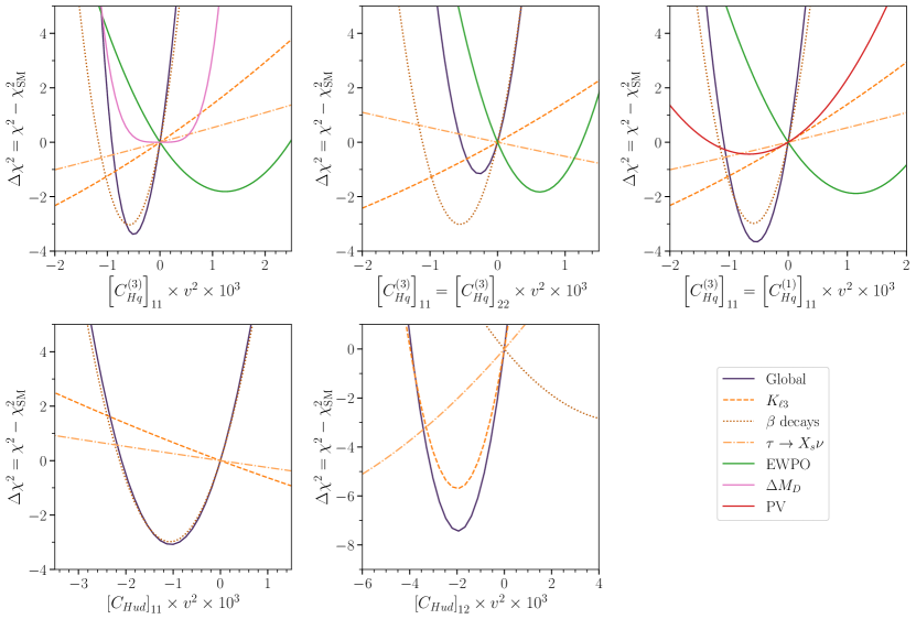
Figure 5: $\Delta\chi^{2}$ w.r.t. the SM as a function of the values of the Wilson coefficients for the 1D scenarios considered in the main text.

2-D scenarios

As we have seen in the previous paragraph, non-zero values of $\left[C_{Hud}\right]_{11}$ and $\left[C_{Hud}\right]_{12}$ lead to modifications of right-handed $W$-$u$-$d$ and $W$-$u$-$s$ couplings and are able to solve and alleviate the tensions within $V_{us}$ and the unitarity deficit, respectively. The resulting preferred regions in the corresponding plane are shown in the left panel of Fig. 6. Note that while inclusive $\tau$ decays are not directly sensitive to right-handed currents, we get a constraint here since they modify the extraction of $V_{us}$ (in our scheme), leading to an indirect sensitivity. On the other hand, despite exclusive $\tau$ decays being more precise, they do not present a constraint here as their theoretical prediction is affected in the same way as $K_{\mu 2}/\pi_{\mu 2}$ used as an input in our scheme.

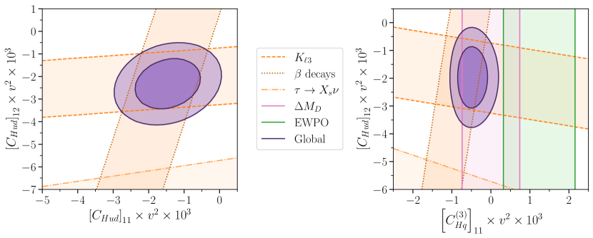
Figure 6: Preferred regions for our two 2-D scenarios, see main text for details.

Alternatively we can consider non-zero values of $\left[C^{(3)}_{Hq}\right]_{11}$ and $\left[C_{Hud}\right]_{12}$ if we aim at explaining both tensions, leading to modifications of the left-handed $W$-$u$-$d$ and a right-handed $W$-$u$-$s$ couplings. The resulting preferred regions are shown on the right of Fig. 6. The best fit points of these two dimensional scenarios together with the pulls are given in Table 4.

3-D scenario

Here we consider the modifications induced if $\left[C^{(3)}_{Hq}\right]_{11}$, $\left[C_{Hud}\right]_{11}$, and $\left[C_{Hud}\right]_{12}$ are simultaneously non-zero. The results are shown in Fig. 7 from where we see that, similar to our 2-D scenarios, there is a strong preference for NP here, but also the significant correlation between left-handed and right-handed $W$-$u$-$d$ modifications. In the appendix D, we consider the 4-D scenarios in which we avoid or weaken the bounds from $\mathit{{D}{}_{\mspace{-3.0mu}\scriptstyle{}}^{\mspace{-1.0mu}\scriptstyle{}}}^{0}$–$\kern 1.99997pt\overline{\kern-1.99997pt\mathit{{D}{}_{\mspace{-3.0mu}\scriptstyle{}}^{\mspace{-1.0mu}\scriptstyle{}}}}{}^{0}$ mixing by adding $\left[C^{(3)}_{Hq}\right]_{11}$ or a $\left[C^{(3)}_{Hq}\right]_{22}$ as free parameters. However, the situation does not change significantly compared to the 3-D scenario as can also be seen from the pulls given in Table 4.

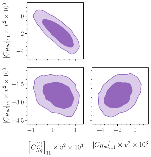
Figure 7: Global fit to our 3-D scenario with non-zero Wilson coefficients $\left[C^{(3)}_{Hq}\right]_{11}$, $\left[C_{Hud}\right]_{11}$, and $\left[C_{Hud}\right]_{12}$.

Summary

The scenarios with modifications of right-handed $W$-$u$-$s$ couplings provide the best improvement relative to the SM (which roughly agrees with the results in Ref. Grossman:2019bzp ) and do not lead to problems in flavour physics or electroweak precision measurements since constraints from $SU(2)_{L}$ invariance are not present. The scenarios with both left-handed and right-handed modifications displays a slightly larger $\Delta\chi^{2}$ (which can be understood by the fact left-handed operators change the EW fit by modifying $Z$-quark couplings) as summarized in Table 4.

EFT Scenario	Best fit point	$-\Delta\chi^{2}$	Pull
$\left[C^{(3)}_{Hq}\right]_{11}$	$-0.50$	$3.3$	$1.8\text{\,}\sigma$
$\left[C^{(3)}_{Hq}\right]_{11}=\left[C^{(3)}_{Hq}\right]_{22}$	$-0.27$	$1.1$	$1.1\text{\,}\sigma$
$\left[C^{(3)}_{Hq}\right]_{11}=\left[C^{(1)}_{Hq}\right]_{11}$	$-0.55$	$3.7$	$1.9\text{\,}\sigma$
$\left[C_{Hud}\right]_{11}$	$-1.0$	$3.1$	$1.8\text{\,}\sigma$
$\left[C_{Hud}\right]_{12}$	$-2.0$	$7.4$	$2.7\text{\,}\sigma$
$\left(\left[C_{Hud}\right]_{11},\left[C_{Hud}\right]_{12}\right)$	$(-1.4,-2.1)$	$13$	$3.2\text{\,}\sigma$
$\left(\left[C^{(3)}_{Hq}\right]_{11},\left[C_{Hud}\right]_{12}\right)$	$(-0.43,-2.0)$	$11$	$2.8\text{\,}\sigma$
$\left(\left[C^{(3)}_{Hq}\right]_{11},\left[C_{Hud}\right]_{11},\left[C_{Hud}\right]_{12}\right)$	$(0.27,-1.9,-2.4)$	$16$	$2.9\text{\,}\sigma$
$\left(\left[C^{(3)}_{Hq}\right]_{11},\left[C^{(3)}_{Hq}\right]_{22},\left[C_{Hud}\right]_{11},\left[C_{Hud}\right]_{12}\right)$	$(0.59,0.76,-2.6,-2.5)$	$17$	$2.9\text{\,}\sigma$
$\left(\left[C^{(3)}_{Hq}\right]_{11},\left[C^{(1)}_{Hq}\right]_{11},\left[C_{Hud}\right]_{11},\left[C_{Hud}\right]_{12}\right)$	$(0.29,0.11,-2.0,-2.4)$	$13$	$2.6\text{\,}\sigma$

Table 4: Best fit points, $\Delta\chi^{2}$ and pulls w.r.t. the SM hypothesis for the various EFT scenarios. The best fit points are in units of $10^{-3}v^{-2}$.

4.2 Vector-like Quark models

Now we examine VLQs coupling to first and second generation quarks in general, and the representations providing a potential solution to the tensions in the CKM matrix in particular. We fix the masses of the VLQs to $2\text{\,}\mathrm{TeV}$, which is compatible with LHC searches ATLAS:2011tvb ; ATLAS:2012apa ; ATLAS:2015lpr ; CMS:2017asf (a recent study has shown that the high-luminosity LHC could exclude a first generation $U$ VLQ at this mass for $\xi^{U}_{1}\gtrsim 0.25$ Cui:2022hjg ). Note that the scaling of the bounds (with the exception of $\Delta F=2$ processes) is just proportional to coupling squared over mass squared, modulus logarithmic effects from the renormalization group evolution. For $\mathit{{D}{}_{\mspace{-3.0mu}\scriptstyle{}}^{\mspace{-1.0mu}\scriptstyle{}}}^{0}$–$\kern 1.99997pt\overline{\kern-1.99997pt\mathit{{D}{}_{\mspace{-3.0mu}\scriptstyle{}}^{\mspace{-1.0mu}\scriptstyle{}}}}{}^{0}$ and kaon mixing, we have included the one-loop matching which becomes relevant for larger masses and breaks the simple scaling observed in the other processes.

In the Figs. 8, 9, 10, 11, 12 and 13 we show in the left-handed panels the preferred regions assuming multiple generations of VLQs, coupling separately to first and second generations quarks, thus avoiding tree-level effects in kaon FCNC processes (despite effects from CKM rotations in $\mathit{{D}{}_{\mspace{-3.0mu}\scriptstyle{}}^{\mspace{-1.0mu}\scriptstyle{}}}^{0}$–$\kern 1.99997pt\overline{\kern-1.99997pt\mathit{{D}{}_{\mspace{-3.0mu}\scriptstyle{}}^{\mspace{-1.0mu}\scriptstyle{}}}}{}^{0}$ mixing). In the right-handed panels the same fit for a single LQ representations, coupling simultaneously to first and second generations quarks is shown. Here, as explained in Sec. 3.3, “CKM” stands for the combined region from the observables listed in Tables 5, 6, 7 and 8 as well as from inclusive $\tau$ decay, while the “$K$ FCNC” includes the observables listed in Table 9. Let us now discuss the various representations separately.

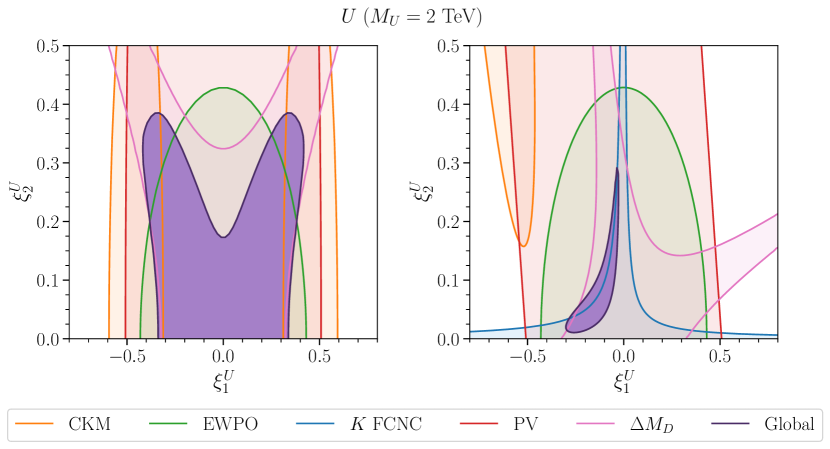
Figure 8: Global fit to $1^{\rm st}$ and $2^{\rm st}$ generation couplings of the VLQ $U$. The left-hand side assumes multiple generations of VLQs, each only coupling to a single generation (i.e. effectively removing constraints from kaon physics), while on the right side this assumption is removed.

$U$ (Fig. 8)

The $SU(2)_{L}$ singlet $U$ (with quantum numbers of a right-handed up-type quark of the SM) leads to modified left-handed $W$ coupling to quarks, so that the CKM tensions favour a non-zero first generation coupling. However, EW precision measurements and data from PV experiments limit the possible size of this coupling, even in the absence of direct contributions to $\mathit{{D}{}_{\mspace{-3.0mu}\scriptstyle{}}^{\mspace{-1.0mu}\scriptstyle{}}}^{0}$–$\kern 1.99997pt\overline{\kern-1.99997pt\mathit{{D}{}_{\mspace{-3.0mu}\scriptstyle{}}^{\mspace{-1.0mu}\scriptstyle{}}}}{}^{0}$ mixing (left panel). In the right panel, the best fit point is at $\xi^{U}_{1}=-0.2,\xi^{U}_{2}=0.045$ with a pull w.r.t. the SM of $2.2\text{\,}\sigma$.

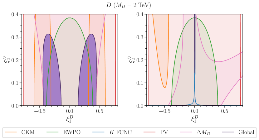
Figure 9: Global fit to $1^{\rm st}$ and $2^{\rm st}$ generation couplings of the VLQ $D$. The left-hand side assumes multiple generations of VLQs, each only coupling to a single generation (i.e. effectively removing constraints from kaon physics), while on the right side this assumption is removed.

$D$ (Fig. 9)

The allowed regions for the Yukawa couplings of $D$ (which has the quantum numbers of a right-handed down-type quark in the SM). We see that while for a single generation kaon FCNC constraints are very severe, (right panel) while in the situation with two generations the allowed regions are much more sizable (left panel). We see that in either case, the data favours a single non-zero coupling, with a best fit at $\xi^{D}_{1}=-0.34$ and a one-dimensional pull w.r.t. the SM of $1.8\text{\,}\sigma$.

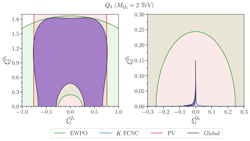
Figure 10: Global fit to $1^{\rm st}$ and $2^{\rm st}$ generation couplings of the VLQ $Q_{5}$. The left-hand side assumes multiple generations of VLQs, each only coupling to a single generation (i.e. effectively removing constraints from kaon physics), while on the right side this assumption is removed.

$Q_{5}$ (Fig. 10)

This $SU(2)_{L}$ doublet VLQ with exotic hypercharge only generates modified $Z$ couplings (but no $W$ couplings) at tree-level, and hence there is no sensitivity to the CKM anomalies. In fact, as the modifications are only to the right-handed $Z$-$d$-$d$ couplings, the current bounds on this VLQ are very weak, as can be seen in the left-hand side of the figure. While PV provides some bounds, there is a small preference for non-zero couplings from EW precision measurements due to the current small tensions in $Z$ width and hadronic cross-section results. Once we allow for a single VLQ to couple to both generations however, we find that kaon physics drastically reduces the allowed region – this occurs due to the RG and matrix element enhancement of $(\bar{s}\gamma^{\mu}P_{L}d)(\bar{s}\gamma_{\mu}P_{R}d)$ four-quark operators in $\epsilon_{K}$.

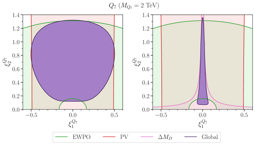
Figure 11: Global fit to $1^{\rm st}$ and $2^{\rm st}$ generation couplings of the VLQ $Q_{7}$. The left-hand side assumes multiple generations of VLQs, each only coupling to a single generation (i.e. effectively removing constraints from kaon physics), while on the right side this assumption is removed.

$Q_{7}$ (Fig. 11)

The results for this VLQ are very similar to the ones for $Q_{5}$, even though this VLQ modifies right-handed $Z$-$u$-$u$ couplings, instead of $Z$-$d$-$d$ ones, although now the main bounds, in case it couples to both first and second generation, originate from $\mathit{{D}{}_{\mspace{-3.0mu}\scriptstyle{}}^{\mspace{-1.0mu}\scriptstyle{}}}^{0}$–$\kern 1.99997pt\overline{\kern-1.99997pt\mathit{{D}{}_{\mspace{-3.0mu}\scriptstyle{}}^{\mspace{-1.0mu}\scriptstyle{}}}}{}^{0}$ mixing.

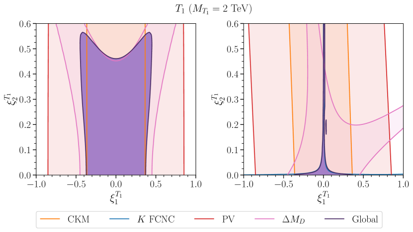
Figure 12: Global fit to $1^{\rm st}$ and $2^{\rm st}$ generation couplings of the VLQ $T_{1}$. The left-hand side assumes multiple generations of VLQs, each only coupling to a single generation (i.e. effectively removing constraints from kaon physics), while on the right side this assumption is removed.

$T_{1}$ (Fig. 12)

This $SU(2)_{L}$ triplet modifies the left-handed charged current, thus affecting the CKM determinations, but in the wrong direction to resolve the first-row unitarity deviations. Therefore, the CKM measurements merely provide a constraint on its interactions, alongside $\mathit{{D}{}_{\mspace{-3.0mu}\scriptstyle{}}^{\mspace{-1.0mu}\scriptstyle{}}}^{0}$–$\kern 1.99997pt\overline{\kern-1.99997pt\mathit{{D}{}_{\mspace{-3.0mu}\scriptstyle{}}^{\mspace{-1.0mu}\scriptstyle{}}}}{}^{0}$ mixing and parity violation. The modifications to $Z$-quark couplings are smaller than in case of the $SU(2)_{L}$ singlet VLQs, and so the corresponding bounds cannot be seen in our region shown. Once we allow the triplet to couple to both generations at once, $\mathit{{D}{}_{\mspace{-3.0mu}\scriptstyle{}}^{\mspace{-1.0mu}\scriptstyle{}}}^{0}$–$\kern 1.99997pt\overline{\kern-1.99997pt\mathit{{D}{}_{\mspace{-3.0mu}\scriptstyle{}}^{\mspace{-1.0mu}\scriptstyle{}}}}{}^{0}$ mixing becomes stronger and kaon constraints are extremely tight.

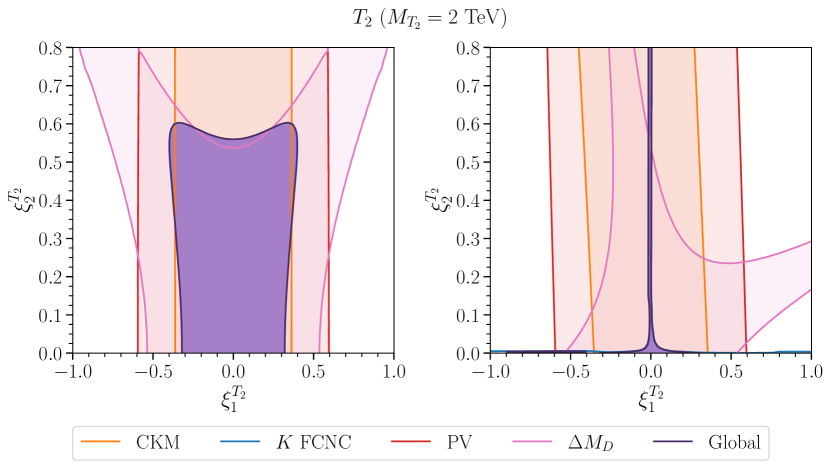
Figure 13: Global fit to $1^{\rm st}$ and $2^{\rm st}$ generation couplings of the VLQ $T_{2}$. The left-hand side assumes multiple generations of VLQs, each only coupling to a single generation (i.e. effectively removing constraints from kaon physics), while on the right side this assumption is removed.

$T_{2}$ (Fig. 13)

The other triplet $T_{2}$ has essentially the same bounds as the first, but bounds from low-energy parity violation are slightly stronger while $\mathit{{D}{}_{\mspace{-3.0mu}\scriptstyle{}}^{\mspace{-1.0mu}\scriptstyle{}}}^{0}$–$\kern 1.99997pt\overline{\kern-1.99997pt\mathit{{D}{}_{\mspace{-3.0mu}\scriptstyle{}}^{\mspace{-1.0mu}\scriptstyle{}}}}{}^{0}$ mixing slightly weaker. Again, once we include couplings to both generations of a single VLQ, kaon decays prove to be very strong and the globally allowed region is quite small.

$Q$ (Fig. 14)

For the $SU(2)_{L}$ doublet $Q$, since it can have both couplings to right-handed up and down quarks, we instead show two fits, for either purely $1^{\rm st}$ or purely $2^{\rm nd}$ generation down quark interactions. The $Q$ doublet is unique in generating modifications to the right-handed $W$ couplings and, as expected from our previous EFT results, there is a strong preference towards non-zero couplings to both right-handed $u$ and $d$ (left) or $u$ and $s$ (right). However, unlike in our simple EFT scenario, the $Q$ field generates additional correlated effects in $Z$ couplings through $SU(2)$ invariance, and so PV and EWPO partially limit the parameter space. In the left panel, the best fit point is $\xi^{u}_{1}=-0.29$, $\xi^{d}_{1}=0.21$ and has a pull w.r.t. the SM of $1.1\text{\,}\sigma$. For the right panel, we find a best fit at $\xi^{u}_{1}=-0.33$, $\xi^{d}_{2}=0.38$ and a pull of $2.1\text{\,}\sigma$.

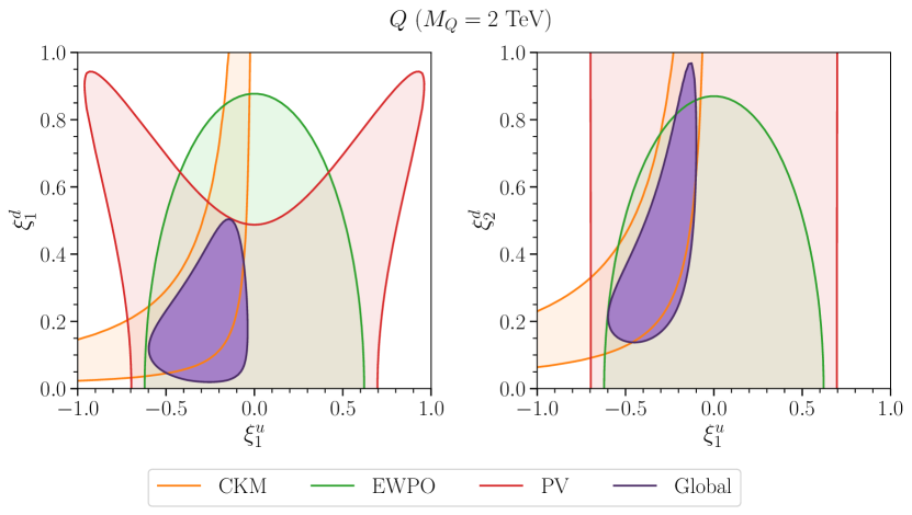
Figure 14: Preferred regions for the VLQ $Q$ with either couplings to $u$ and $d$ (left) or $u$ and $s$ (right).

VLQs and tensions in the Cabibbo angle

In our SMEFT analysis we saw that resolving the CAA via modified gauge boson couplings requires NP in $\left[C^{(3)}_{Hq}\right]_{11}$ and/or $\left[C_{Hud}\right]_{11}$ as well as in $\left[C_{Hud}\right]_{12}$ for the $V_{us}$ tension. From the tree-level matching of VLQs on the SMEFT (see Eq. (3.6)), we see that only the $SU(2)_{L}$ doublet $Q$ can generate the coefficients $C_{Hud}$ that generate right-handed $W$ couplings. Furthermore, for a single generation of the doublet, NP in the right-handed $W$-$u$-$d$ and $W$-$u$-$s$ vertices (at the same time) lead to significant NP in right-handed $Z$-$d$-$s$ couplings, stringently constrained by $\epsilon_{K}$ Endo:2016tnu ; Bobeth:2017xry . Updating their result, we find that a single $Q$ doublet coupled to both $d$ and $s$ would have to obey $M_{Q}/\sqrt{\xi^{d}_{1}\xi^{d}_{2}}>$175\text{\,}\mathrm{TeV}$$ to be consistent with experiment, and therefore far too heavy to be relevant to the CAA.

Thus, a full explanation of the tensions in the Cabibbo angle determination require a modified $W$-$u$-$d$ and $W$-$u$-$s$ coupling and thus multiple generations of $Q$. Similarly, one can solve the CAA via a modified left-handed $W$-$u$-$d$ coupling and a right-handed $W$-$u$-$s$ coupling which again requires at least two VLQs. This means that a full solution of the CAA demands the presence of at least two VLQs.

5 Conclusions

In this article we studied modified couplings of light quarks to EW gauge bosons, both in the SMEFT and in models with VLQs. We paid particular attention to the different determinations of the Cabibbo angle that are in disagreement with each other, pointing towards such modified $W$ couplings to quarks. We performed a global analysis using smelli, taking into account the constraints for EW precision and flavour observables.

In more detail, we first summarised the current status of the determinations of the CKM elements $V_{ud}$ and $V_{us}$. For $V_{ud}$, where super-allowed $\beta$ decays continue to provide the most precise determination, neutron decays is quickly approaching competitively, and its current central value is only slightly larger than (and therefore perfectly consistent with) the one from super-allowed decays. For the direct determination of $V_{us}$ the leading decay mode is $K\to\pi\ell\nu$ as there are still questions to be resolved regarding theory prediction for inclusive $\tau$ decays and how this should be applied to data. Finally, the ratio $V_{us}$/$V_{ud}$ is dominated by $K\to\mu\nu/\pi\to\mu\nu$ as the ratios $\tau\to K\nu/\tau\to\pi\nu$ and $K\to\pi\ell\nu/\pi\to\pi e\nu$ are currently limited by the experimental data. We tested the CKM unitarity prediction of the SM by taking each pair of the best measurements individually, and find that it is violated between $1.8\text{\,}\sigma$ and $3.3\text{\,}\sigma$ (see Eq. (2.13)). This agrees with the result of the global fit to all available data where we find the unitarity violation at the $2.8\text{\,}\sigma$ level (see Eq. (2.12)). Furthermore, a tension between the different determinations of $V_{us}$ exists, which can only be explained by non-standard right-handed interactions and can be tested through a $K\to\pi\mu\nu/K\to\mu\nu$ measurement in the near future by NA62 Cirigliano:2022yyo .

In our global SMEFT fit, we found that several scenarios can solve or alleviate the tensions in the determinations of the Cabibbo angle, as summarized in Table 4. The simplest and least problematic case is that of right-handed charged currents (both in $W$-$u$-$d$ and $W$-$u$-$s$ couplings) which can bring all the main determinations into agreement without being in conflict with EW precision or flavour observables, and is therefore favoured over the SM hypothesis by $3.2\text{\,}\sigma$ ($2.7\text{\,}\sigma$) in the best 2-D (1-D) scenario. Other scenarios with modified left-handed charged currents (only) are also preferred over the SM hypothesis, but cannot account for the discrepancies within $V_{us}$ and face constraints from EW precision measurements as well as $\mathit{{D}{}_{\mspace{-3.0mu}\scriptstyle{}}^{\mspace{-1.0mu}\scriptstyle{}}}^{0}$–$\kern 1.99997pt\overline{\kern-1.99997pt\mathit{{D}{}_{\mspace{-3.0mu}\scriptstyle{}}^{\mspace{-1.0mu}\scriptstyle{}}}}{}^{0}$ mixing. While the latter bounds can be weakened or avoided by considering a $U(2)$ flavour symmetry or a specific combination of Wilson coefficients, respectively, the global fit displays a maximal pull of $1.9\sigma$ if only left-handed currents are considered.

The most natural extension of the SM that leads to modified EW gauge couplings to quarks are VLQs. They affect these couplings already at tree-level and are also theoretically well-motivated, e.g., by grand unified theories, composite and extra-dimensional models and little Higgs models etc. We first matched the different VLQ representations under the SM gauge group on the SMEFT (at tree-level for the charged current and EW precision observables and at loop-level for $\Delta F=2$ processes) and used these results to calculate the relevant effects in the related observables. We then performed a global fit for the different representations of VLQs, taking into account couplings to first and second generation quarks. While a single VLQ coupling simultaneously to first and second generation quarks will lead to FCNCs and is hence very constrained, these bounds can be avoided or weakened for multiple generations of VLQs.

The $SU(2)_{L}$ singlet VLQs can improve the fit w.r.t. the CAA, but EW precision and $\mathit{{D}{}_{\mspace{-3.0mu}\scriptstyle{}}^{\mspace{-1.0mu}\scriptstyle{}}}^{0}$–$\kern 1.99997pt\overline{\kern-1.99997pt\mathit{{D}{}_{\mspace{-3.0mu}\scriptstyle{}}^{\mspace{-1.0mu}\scriptstyle{}}}}{}^{0}$ mixing (as well as PV measurements for the $U$) prevent a better description of data. The $SU(2)_{L}$ triplet VLQs generate the wrong sign to match our left-handed EFT scenario for the CAA, so that here CKM unitarity acts as a constraint but the tension cannot be explained. The $SU(2)_{L}$ doublets with non-SM-like hypercharges do not contribute to CKM observables, as they only generate modified $Z$ but not $W$ couplings to quarks. The heavy SM-like doublet $Q$ proves the most interesting case, as this is the only VLQ that generates the right-handed $W$ couplings to quarks. As expected from our EFT fits, this VLQ is strongly favoured by the CKM measurements, but now faces bounds from EWPO and PV as modified right-handed $Z$ couplings to quarks are also induced, removing some of the parameter space and reducing the improvement to the $\chi^{2}$ of the fit to data. In fact, if one compares the $\left[C_{Hud}\right]_{11}$ scenario with a best fit pull of $1.8\text{\,}\sigma$ to the corresponding $Q$ UV model with only $1.1\text{\,}\sigma$, and similarly the $\left[C_{Hud}\right]_{12}$ scenario has a best fit pull of $2.7\text{\,}\sigma$, compared to only $2.1\text{\,}\sigma$ in the second $Q$ scenario. We note however the best fit points remains consistent with the right-handed EFT fit.

In conclusion, the tensions related to the determination of the Cabibbo angle can be most easily explained by new physics leading to right-handed charged currents and therefore by vector-like quark $Q$. Therefore, while collider bounds for third generations VLQs have been well studied, the CAA provides strong motivation for searches for VLQs coupling to first and second generation quarks.

Appendix A SMEFT matching

Here we present the matching expressions at one-loop for the four-quarks operators which contribute to $\mathit{{D}{}_{\mspace{-3.0mu}\scriptstyle{}}^{\mspace{-1.0mu}\scriptstyle{}}}^{0}$–$\kern 1.99997pt\overline{\kern-1.99997pt\mathit{{D}{}_{\mspace{-3.0mu}\scriptstyle{}}^{\mspace{-1.0mu}\scriptstyle{}}}}{}^{0}$ mixing, which we calculated using matchmakereft Carmona:2021xtq .

$$\left[C_{qq}^{(1)}\right]_{ijkl} =\begin{aligned} &-\frac{\xi^{U*}_{fi}\xi^{U}_{fj}\xi^{U*}_{gk}\xi^{U}_{gl}}{256\pi^{2}M_{U}^{2}}+\frac{3(Y^{u}Y^{u,\dagger})_{ij}\xi^{U*}_{fk}\xi^{U}_{fl}}{512\pi^{2}M_{U}^{2}}+\frac{3(Y^{u}Y^{u,\dagger})_{kl}\xi^{U*}_{fi}\xi^{U}_{fj}}{512\pi^{2}M_{U}^{2}}\\ &-\frac{\xi^{D*}_{fi}\xi^{D}_{fj}\xi^{D*}_{gk}\xi^{D}_{gl}}{256\pi^{2}M_{D}^{2}}-\frac{3(Y^{u}Y^{u,\dagger})_{ij}\xi^{D*}_{fk}\xi^{D}_{fl}}{512\pi^{2}M_{D}^{2}}-\frac{3(Y^{u}Y^{u,\dagger})_{kl}\xi^{D*}_{fi}\xi^{D}_{fj}}{512\pi^{2}M_{D}^{2}}\\ &-\frac{9\xi^{T_{1}*}_{i}\xi^{T_{2}}_{j}\xi^{T_{1}*}_{k}\xi^{T_{2}}_{l}}{4096\pi^{2}M_{T_{1}}^{2}}-\frac{9(Y^{u}Y^{u,\dagger})_{ij}\xi^{T_{1}*}_{fk}\xi^{T_{1}}_{fl}}{2048\pi^{2}M_{T_{1}}^{2}}-\frac{9(Y^{u}Y^{u,\dagger})_{kl}\xi^{T_{1}*}_{fi}\xi^{T_{1}}_{fj}}{2048\pi^{2}M_{T_{1}}^{2}}\\ &-\frac{9\xi^{T_{2}*}_{fi}\xi^{T_{2}}_{fj}\xi^{T_{2}*}_{gk}\xi^{T_{2}}_{gl}}{4096\pi^{2}M_{T_{2}}^{2}}+\frac{9(Y^{u}Y^{u,\dagger})_{ij}\xi^{T_{2}*}_{fk}\xi^{T_{2}}_{fl}}{2048\pi^{2}M_{T_{2}}^{2}}+\frac{9(Y^{u}Y^{u,\dagger})_{kl}\xi^{T_{2}*}_{fi}\xi^{T_{2}}_{fj}}{2048\pi^{2}M_{T_{2}}^{2}}\,,\end{aligned}$$ (A.1)

$$\left[C_{qq}^{(3)}\right]_{ijkl} =\begin{aligned} &-\frac{\xi^{U*}_{fi}\xi^{U}_{fj}\xi^{U*}_{gk}\xi^{U}_{gl}}{256\pi^{2}M_{U}^{2}}+\frac{3(Y^{u}Y^{u,\dagger})_{ij}\xi^{U*}_{fk}\xi^{U}_{fl}}{512\pi^{2}M_{U}^{2}}+\frac{3(Y^{u}Y^{u,\dagger})_{kl}\xi^{U*}_{fi}\xi^{U}_{fj}}{512\pi^{2}M_{U}^{2}}\\ &-\frac{\xi^{D*}_{fi}\xi^{D}_{fj}\xi^{D*}_{gk}\xi^{D}_{gl}}{256\pi^{2}M_{D}^{2}}+\frac{3(Y^{u}Y^{u,\dagger})_{ij}\xi^{D*}_{fk}\xi^{D}_{fl}}{512\pi^{2}M_{D}^{2}}+\frac{3(Y^{u}Y^{u,\dagger})_{kl}\xi^{D*}_{fi}\xi^{D}_{fj}}{512\pi^{2}M_{D}^{2}}\\ &-\frac{\xi^{T_{1}*}_{fi}\xi^{T_{2}}_{fj}\xi^{T_{1}*}_{gk}\xi^{T_{2}}_{gl}}{4096\pi^{2}M_{T_{1}}^{2}}-\frac{3(Y^{u}Y^{u,\dagger})_{ij}\xi^{T_{1}*}_{fk}\xi^{T_{1}}_{fl}}{2048\pi^{2}M_{T_{1}}^{2}}-\frac{3(Y^{u}Y^{u,\dagger})_{kl}\xi^{T_{1}*}_{fi}\xi^{T_{1}}_{fj}}{2048\pi^{2}M_{T_{1}}^{2}}\\ &-\frac{\xi^{T_{2}*}_{fi}\xi^{T_{2}}_{fj}\xi^{T_{2}*}_{gk}\xi^{T_{2}}_{gl}}{4096\pi^{2}M_{T_{2}}^{2}}-\frac{3(Y^{u}Y^{u,\dagger})_{ij}\xi^{T_{2}*}_{fk}\xi^{T_{2}}_{fl}}{2048\pi^{2}M_{T_{2}}^{2}}-\frac{3(Y^{u}Y^{u,\dagger})_{kl}\xi^{T_{2}*}_{fi}\xi^{T_{2}}_{fj}}{2048\pi^{2}M_{T_{2}}^{2}}\,,\end{aligned}$$ (A.2)

$$\left[C_{qu}^{(1)}\right]_{ijkl} =\begin{aligned} &-\frac{3(Y^{u,\dagger}Y^{u})_{kl}\xi^{U*}_{fi}\xi^{U}_{fj}}{128\pi^{2}M_{U}^{2}}-\frac{Y^{u}_{il}Y^{u,\dagger}_{kj}\xi^{U*}_{fm}\xi^{U}_{fm}}{96\pi^{2}M_{U}^{2}}+\frac{3(Y^{u,\dagger}Y^{u})_{kl}\xi^{D*}_{fi}\xi^{D}_{fj}}{128\pi^{2}M_{D}^{2}}\\ &+\frac{Y^{u}_{il}\xi^{D}_{fj}(Y^{u,\dagger}\xi^{D\dagger})_{kf}}{192\pi^{2}M_{D}^{2}}+\frac{\xi^{D*}_{fi}Y^{u,\dagger}_{kj}(\xi^{D}Y^{u})_{fl}}{192\pi^{2}M_{D}^{2}}-\frac{Y^{u}_{il}Y^{u,\dagger}_{kj}\xi^{D*}_{fm}\xi^{D}_{fm}}{96\pi^{2}M_{D}^{2}}\\ &-\frac{3(Y^{u}Y^{u,\dagger})_{ij}\xi^{u*}_{fk}\xi^{u}_{fl}}{128\pi^{2}M_{Q}^{2}}-\frac{Y^{u}_{il}Y^{u,\dagger}_{jk}\xi^{d*}_{fm}\xi^{d}_{fm}}{96\pi^{2}M_{Q}^{2}}-\frac{Y^{u}_{il}Y^{u,\dagger}_{jk}\xi^{u*}_{fm}\xi^{u}_{fm}}{96\pi^{2}M_{Q}^{2}}-\frac{\xi^{Q_{5}}_{fm}\xi^{Q_{5}*}_{fm}Y^{u}_{il}Y^{u,\dagger}_{kj}}{96\pi^{2}M_{Q_{5}}^{2}}\\ &+\frac{3(Y^{u}Y^{u,\dagger})_{ij}\xi^{Q_{7}*}_{fk}\xi^{Q_{7}}_{fl}}{128\pi^{2}M_{Q_{7}}^{2}}-\frac{Y^{u}_{il}(\xi^{Q_{7}}Y^{u,\dagger})_{fj}\xi^{Q_{7}*}_{fk}}{192\pi^{2}M_{Q_{7}}^{2}}-\frac{(Y^{u}\xi^{Q_{7}\dagger})_{fi}Y^{u,\dagger})_{kj}\xi^{Q_{7}}_{fl}}{192\pi^{2}M_{Q_{7}}^{2}}\\ &-\frac{\xi^{Q_{7}}_{fm}\xi^{Q_{7}*}_{fm}Y^{u}_{il}Y^{u,\dagger}_{kj}}{96\pi^{2}M_{Q_{7}}^{2}}\\ &+\frac{9(Y^{u,\dagger}Y^{u})_{kl}\xi^{T_{1}*}_{fi}\xi^{T_{1}}_{fj}}{512\pi^{2}M_{T_{1}}^{2}}-\frac{Y^{u}_{il}\xi^{D}_{fj}(Y^{u,\dagger}\xi^{T_{1}\dagger})_{kf}}{256\pi^{2}M_{T_{1}}^{2}}-\frac{\xi^{T_{1}*}_{fi}Y^{u,\dagger}_{kj}(\xi^{T_{1}}Y^{u})_{fl}}{256\pi^{2}M_{T_{1}}^{2}}\\ &-\frac{Y^{u}_{il}Y^{u,\dagger}_{kj}\xi^{T_{1}*}_{fm}\xi^{T_{1}}_{fm}}{128\pi^{2}M_{T_{1}}^{2}}-\frac{9(Y^{u,\dagger}Y^{u})_{kl}\xi^{T_{2}*}_{fi}\xi^{T_{2}}_{fj}}{512\pi^{2}M_{T_{2}}^{2}}-\frac{Y^{u}_{il}Y^{u,\dagger}_{kj}\xi^{T_{2}*}_{fm}\xi^{T_{2}}_{fm}}{128\pi^{2}M_{T_{2}}^{2}}\,,\end{aligned}$$ (A.3)

$$\left[C_{qu}^{(8)}\right]_{ijkl} =\begin{aligned} &-\frac{Y^{u}_{il}Y^{u,\dagger}_{kj}\xi^{U*}_{fm}\xi^{U}_{fm}}{16\pi^{2}M_{U}^{2}}\\ &+\frac{Y^{u}_{il}\xi^{D}_{fj}(Y^{u,\dagger}\xi^{D\dagger})_{kf}}{32\pi^{2}M_{D}^{2}}+\frac{\xi^{D*}_{fi}Y^{u,\dagger}_{kj}(\xi^{D}Y^{u})_{fl}}{32\pi^{2}M_{D}^{2}}-\frac{Y^{u}_{il}Y^{u,\dagger}_{kj}\xi^{D*}_{fm}\xi^{D}_{fm}}{16\pi^{2}M_{D}^{2}}\\ &-\frac{Y^{u}_{il}Y^{u,\dagger}_{jk}\xi^{d*}_{fm}\xi^{d}_{fm}}{16\pi^{2}M_{Q}^{2}}-\frac{Y^{u}_{il}Y^{u,\dagger}_{jk}\xi^{u*}_{fm}\xi^{u}_{fm}}{16\pi^{2}M_{Q}^{2}}-\frac{\xi^{Q_{5}}_{fm}\xi^{Q_{5}*}_{fm}Y^{u}_{il}Y^{u,\dagger}_{kj}}{16\pi^{2}M_{Q_{5}}^{2}}\\ &-\frac{Y^{u}_{il}(\xi^{Q_{7}}Y^{u,\dagger})_{fj}\xi^{Q_{7}*}_{fk}}{32\pi^{2}M_{Q_{7}}^{2}}-\frac{(Y^{u}\xi^{Q_{7}\dagger})_{if}Y^{u,\dagger})_{kj}\xi^{Q_{7}}_{fl}}{32\pi^{2}M_{Q_{7}}^{2}}-\frac{\xi^{Q_{7}}_{fm}\xi^{Q_{7}*}_{fm}Y^{u}_{il}Y^{u,\dagger}_{kj}}{16\pi^{2}M_{Q_{7}}^{2}}\\ &+\frac{Y^{u}_{il}\xi^{T_{1}}_{fj}(Y^{u,\dagger}\xi^{T_{1}\dagger})_{kf}}{128\pi^{2}M_{T_{1}}^{2}}+\frac{\xi^{T_{1}*}_{fi}Y^{u,\dagger}_{kj}(\xi^{T_{1}}Y^{u})_{fl}}{128\pi^{2}M_{T_{1}}^{2}}-\frac{Y^{u}_{il}Y^{u,\dagger}_{kj}\xi^{T_{1}*}_{fm}\xi^{T_{1}}_{fm}}{64\pi^{2}M_{T_{1}}^{2}}\\ &-\frac{3Y^{u}_{il}Y^{u,\dagger}_{kj}\xi^{T_{2}*}_{fm}\xi^{T_{2}}_{fm}}{64\pi^{2}M_{T_{2}}^{2}}\,,\end{aligned}$$ (A.4)

$$\left[C_{uu}\right]_{ijkl} =\begin{aligned} &-\frac{\xi^{u*}_{fi}\xi^{u}_{fj}\xi^{u*}_{gk}\xi^{u}_{gl}}{64\pi^{2}M_{Q}^{2}}+\frac{3(Y^{u,\dagger}Y^{u})_{ij}\xi^{u*}_{fk}\xi^{u}_{fl}}{128\pi^{2}M_{Q}^{2}}+\frac{3(Y^{u,\dagger}Y^{u})_{kl}\xi^{u*}_{fi}\xi^{u}_{fj}}{128\pi^{2}M_{Q}^{2}}\\ &-\frac{\xi^{q_{7}*}_{fi}\xi^{Q_{7}}_{fj}\xi^{Q_{7}*}_{gk}\xi^{Q_{7}}_{gl}}{64\pi^{2}M_{Q_{7}}^{2}}-\frac{3(Y^{u,\dagger}Y^{u})_{ij}\xi^{Q_{7}*}_{fk}\xi^{Q_{7}}_{fl}}{128\pi^{2}M_{Q_{7}}^{2}}-\frac{3(Y^{u,\dagger}Y^{u})_{kl}\xi^{Q_{7}*}_{fi}\xi^{Q_{7}}_{fj}}{128\pi^{2}M_{Q_{7}}^{2}}\,,\end{aligned}$$ (A.5)

where $f,g$ are flavour indices for the new VLQs, we have assumed equal masses for multiple generations of VLQs to simplify the loop functions, and the matching conditions have been specified at the VLQ mass scale, such that $\ln(\mu^{2}/M^{2})$ terms vanish.

In the down-basis we have adopted, it is useful to note that products of Yukawa matrices can be simplified as

$$\left(Y^{u}Y^{u,\dagger}\right)_{ij}=y_{t}^{2}V_{*}{3i}V_{3j}+\mathcal{O}\left(y_{c}^{2}\right)\,,\quad\left(Y^{u,\dagger}Y^{u}\right)_{ij}=y_{t}^{2}\delta_{3i}\delta_{3j}+\mathcal{O}\left(y_{c}^{2}\right)\,.$$ (A.6)

Note though that we keep the full expressions in our numerical analyses.

Appendix B Effective CKM elements

In the presence of non-zero SMEFT coefficients, the effective CKM elements as extracted from $\beta$ decay, semi-leptonic kaon decay, and leptonic kaon and pion decay are:

$$V_{ud}^{\beta} =V_{ud}+v^{2}\left[V_{\text{CKM}}\cdot C^{(3)}_{Hq}\right]_{11}+\frac{v^{2}}{2}\left[C_{Hud}\right]_{11}\,,$$ (B.1)

$$V_{us}^{K_{\ell 3}} =V_{us}+v^{2}\left[V_{\text{CKM}}\cdot C^{(3)}_{Hq}\right]_{12}+\frac{v^{2}}{2}\left[C_{Hud}\right]_{12}\,,$$ (B.2)

$$V_{uq}^{M_{\mu 2}} =V_{uq}+v^{2}\left[V_{\text{CKM}}\cdot C^{(3)}_{Hq}\right]_{1q}-\frac{v^{2}}{2}\left[C_{Hud}\right]_{1q}\,,$$ (B.3)

for $q=d,s$ and $M=K,\pi$ in the final equation. (Notice that we obviously see here how right-handed currents are needed to resolve the tension between $V_{us}$ determinations.)

Rearranging, and assuming small NP contributions in only the four coefficients $\left[C^{(3)}_{Hq}\right]_{11,12}$ and $\left[C_{Hud}\right]_{11,12}$ we find:

$$V_{ud} =V_{ud}^{\beta}-v^{2}\left(V_{ud}^{\beta}\left[C^{(3)}_{Hq}\right]_{11}+\frac{1}{2}\left[C_{Hud}\right]_{11}\right)\,,$$ (B.4)

$$V_{us} =V_{us}^{K_{\ell 3}}-v^{2}\left(V_{ud}^{\beta}\left[C^{(3)}_{Hq}\right]_{12}+\frac{1}{2}\left[C_{Hud}\right]_{12}\right)\,,$$ (B.5)

$$\frac{V_{us}}{V_{ud}} =\frac{V_{us}^{K_{\mu 2}}-v^{2}\left(V_{ud}\left[C^{(3)}_{Hq}\right]_{12}-\frac{1}{2}\left[C_{Hud}\right]_{12}\right)}{V_{ud}^{\pi_{\mu 2}}-v^{2}\left(V_{ud}\left[C^{(3)}_{Hq}\right]_{11}-\frac{1}{2}\left[C_{Hud}\right]_{11}\right)}$$ (B.6)

$$=\left(\frac{V_{us}}{V_{ud}}\right)^{M_{\mu 2}}\!\!\!\!+v^{2}\left(\left(\frac{V_{us}}{V_{ud}}\right)^{M_{\mu 2}}\left[C^{(3)}_{Hq}\right]_{11}-\left[C^{(3)}_{Hq}\right]_{12}-\left(\frac{V_{us}}{V_{ud}}\right)^{M_{\mu 2}}\frac{\left[C_{Hud}\right]_{11}}{2V_{ud}^{\beta}}+\frac{\left[C_{Hud}\right]_{12}}{2V_{ud}^{\beta}}\right)\,.$$ (B.7)

Appendix C smelli observables

In Tables 5, 6, 7, 8, 9 and 10 we list the observables shown in our global fits, along with the relevant experimental measurements and theory papers used in the computation.

Observable	Exp.	Theory	Observable	Exp.	Theory
$\text{BR}(K_{L}\to\pi^{+}e^{+}\nu)$	ParticleDataGroup:2022pth	Antonelli:2010yf ; Bernard:2009zm	$\text{BR}(K_{S}\to\pi^{+}e^{+}\nu)$	KLOE-2:2022dot	Antonelli:2010yf ; Bernard:2009zm
$\text{BR}(K^{+}\to\pi^{0}e^{+}\nu)$	ParticleDataGroup:2022pth	Antonelli:2010yf ; Bernard:2009zm	$\text{BR}(K_{L}\to\pi^{+}\mu^{+}\nu)$	ParticleDataGroup:2022pth	Antonelli:2010yf ; Bernard:2009zm
$\text{BR}(K_{S}\to\pi^{+}\mu^{+}\nu)$	KLOE-2:2019rev	Antonelli:2010yf ; Bernard:2009zm	$\text{BR}(K^{+}\to\pi^{0}\mu^{+}\nu)$	ParticleDataGroup:2022pth	Antonelli:2010yf ; Bernard:2009zm
$\ln(C)(K^{+}\to\pi^{0}\mu^{+}\nu)$	Moulson:2014cra	Antonelli:2010yf ; Bernard:2009zm	$R_{T}(K^{+}\to\pi^{0}\mu^{+}\nu)$	Yushchenko:2003xz	Antonelli:2010yf ; Bernard:2009zm

Table 5: The “$K_{\ell 3}$” observables used in smelli, along with the relevant experimental measurements and theory papers used in the computation.

Observable	Exp.	Theory	Observable	Exp.	Theory
$\mathcal{F}t({}^{10}\text{C})$	Hardy:2020qwl	Gonzalez-Alonso:2018omy	$\mathcal{F}t({}^{14}\text{O})$	Hardy:2020qwl	Gonzalez-Alonso:2018omy
$\mathcal{F}t({}^{22}\text{Mg})$	Hardy:2020qwl	Gonzalez-Alonso:2018omy	$\mathcal{F}t({}^{26m}\text{Al})$	Hardy:2020qwl	Gonzalez-Alonso:2018omy
$\mathcal{F}t({}^{34}\text{Cl})$	Hardy:2020qwl	Gonzalez-Alonso:2018omy	$\mathcal{F}t({}^{34}\text{Ar})$	Hardy:2020qwl	Gonzalez-Alonso:2018omy
$\mathcal{F}t({}^{38m}\text{K})$	Hardy:2020qwl	Gonzalez-Alonso:2018omy	$\mathcal{F}t({}^{38}\text{Ca})$	Hardy:2020qwl	Gonzalez-Alonso:2018omy
$\mathcal{F}t({}^{42}\text{Sc})$	Hardy:2020qwl	Gonzalez-Alonso:2018omy	$\mathcal{F}t({}^{46}\text{V})$	Hardy:2020qwl	Gonzalez-Alonso:2018omy
$\mathcal{F}t({}^{50}\text{Mn})$	Hardy:2020qwl	Gonzalez-Alonso:2018omy	$\mathcal{F}t({}^{54}\text{Co})$	Hardy:2020qwl	Gonzalez-Alonso:2018omy
$\mathcal{F}t({}^{62}\text{Ga})$	Hardy:2020qwl	Gonzalez-Alonso:2018omy	$\mathcal{F}t({}^{74}\text{Rb})$	Hardy:2020qwl	Gonzalez-Alonso:2018omy
$\tau_{n}$	UCNt:2021pcg	Gonzalez-Alonso:2018omy	$\tilde{A}_{n}$	Markisch:2018ndu ; Brown:2017mhw ; Mund:2012fq	Gonzalez-Alonso:2018omy
$R_{n}$	Kozela:2011mc	Gonzalez-Alonso:2018omy	$\lambda_{AB}$	Mostovoi:2001ye	Gonzalez-Alonso:2018omy
$a_{n}$	Gonzalez-Alonso:2018omy	Gonzalez-Alonso:2018omy	$\tilde{a}_{n}$	Darius:2017arh	Gonzalez-Alonso:2018omy
$\tilde{B}_{n}$	Gonzalez-Alonso:2018omy	Gonzalez-Alonso:2018omy	$D_{n}$	Gonzalez-Alonso:2018omy	Gonzalez-Alonso:2018omy

Table 6: The “beta” observables used in smelli, along with the relevant experimental measurements and theory papers used in the computation.

Observable	Exp.	Observable	Exp.
$\text{BR}(\tau^{+}\to\pi^{+}\bar{\nu})$	ParticleDataGroup:2022pth	$\text{BR}(\tau^{+}\to K^{+}\bar{\nu})$	ParticleDataGroup:2022pth

Table 7: The exclusive $\tau$ decays observables used in smelli, along with the relevant experimental measurements and theory papers used in the computation.

Observable	Exp.	Theory	Observable	Exp.	Theory
$\text{BR}(D^{+}\to e^{+}\nu_{e})$	ParticleDataGroup:2022pth		$\text{BR}(D^{+}\to\mu^{+}\nu_{\mu})$	ParticleDataGroup:2022pth
$\text{BR}(D^{+}\to\tau^{+}\nu_{\tau})$	ParticleDataGroup:2022pth		$\text{BR}(D_{s}\to e^{+}\nu_{e})$	ParticleDataGroup:2022pth
$\text{BR}(D_{s}\to\mu^{+}\nu_{\mu})$	ParticleDataGroup:2022pth		$\text{BR}(D_{s}\to\tau^{+}\nu_{\tau})$	ParticleDataGroup:2022pth
$\text{BR}(D^{0}\to\pi^{-}\mu^{+}\nu_{\mu})$	ParticleDataGroup:2022pth	Gubernari:2018wyi	$\text{BR}(D^{0}\to\pi^{-}e^{+}\nu_{e})$	ParticleDataGroup:2022pth	Gubernari:2018wyi
$\text{BR}(D^{0}\to K^{-}e^{+}\nu_{e})$	ParticleDataGroup:2022pth	Gubernari:2018wyi	$\text{BR}(D^{0}\to K^{-}\mu^{+}\nu_{\mu})$	ParticleDataGroup:2022pth	Gubernari:2018wyi
$\langle\text{BR}\rangle(D^{0}\to\pi^{-}e^{+}\nu_{e})$	CLEO:2009svp ; BESIII:2015tql	Gubernari:2018wyi	$\text{BR}(D^{+}\to\pi^{0}\mu^{+}\nu_{\mu})$	ParticleDataGroup:2022pth	Gubernari:2018wyi
$\langle\text{BR}\rangle(D^{0}\to K^{-}e^{+}\nu_{e})$	CLEO:2009svp ; BESIII:2015tql	Gubernari:2018wyi	$\text{BR}(D^{+}\to K^{0}\mu^{+}\nu_{\mu})$	ParticleDataGroup:2022pth	Gubernari:2018wyi
$\langle\text{BR}\rangle(D^{+}\to K^{0}e^{+}\nu_{e})$	CLEO:2009svp ; BESIII:2017ylw	Gubernari:2018wyi	$\text{BR}(D^{+}\to\pi^{0}e^{+}\nu_{e})$	ParticleDataGroup:2022pth	Gubernari:2018wyi
$\langle\text{BR}\rangle(D^{+}\to\pi^{0}e^{+}\nu_{e})$	CLEO:2009svp ; BESIII:2017ylw	Gubernari:2018wyi	$\text{BR}(D^{+}\to K^{0}e^{+}\nu_{e})$	ParticleDataGroup:2022pth	Gubernari:2018wyi

Table 8: The $D$ decay observables used in smelli, along with the relevant experimental measurements and theory papers used in the computation. $\langle\text{BR}\rangle$ are $q^{2}$-binned branching ratios.

Observable	Exp.	Theory	Observable	Exp.	Theory
$\text{BR}(K^{+}\to\pi^{+}\nu\bar{\nu})$	NA62:2021zjw	Brod:2010hi ; Buras:2006gb ; Buchalla:1998ba ; Isidori:2005xm ; Mescia:2007kn	$\text{BR}(K_{L}\to\pi^{0}\nu\bar{\nu})$	Ahn:2018mvc	Brod:2010hi ; Buras:2006gb ; Buchalla:1998ba ; Isidori:2005xm ; Mescia:2007kn
$\text{BR}(K_{L}\to e^{+}e^{-})$	ParticleDataGroup:2022pth	Bobeth:2013uxa ; Gorbahn:2006bm ; Chobanova:2017rkj	$\text{BR}(K_{S}\to e^{+}e^{-})$	ParticleDataGroup:2022pth	Bobeth:2013uxa ; Gorbahn:2006bm ; Chobanova:2017rkj
$\text{BR}(K_{L}\to\mu^{+}\mu^{-})$	ParticleDataGroup:2022pth	Bobeth:2013uxa ; Gorbahn:2006bm ; Chobanova:2017rkj	$\text{BR}(K_{S}\to\mu^{+}\mu^{-})$	LHCb:2020ycd	Bobeth:2013uxa ; Gorbahn:2006bm ; Chobanova:2017rkj
$|\epsilon_{K}|$	ParticleDataGroup:2022pth	Blum:2011ng ; Brod:2011ty ; Brod:2010mj ; Carrasco:2015pra

Table 9: The “$K$ FCNC” observables used in smelli, along with the relevant experimental measurements and theory papers used in the computation.

Observable	Exp.	Theory	Observable	Exp.	Theory
$\Gamma_{Z}$	Janot:2019oyi	Brivio:2017vri ; Freitas:2014hra	$\sigma_{\text{had}}^{0}$	Janot:2019oyi	Brivio:2017vri ; Freitas:2014hra
$R_{e}^{0}$	Janot:2019oyi	Brivio:2017vri ; Freitas:2014hra	$R_{\mu}^{0}$	Janot:2019oyi	Brivio:2017vri ; Freitas:2014hra
$R_{\tau}^{0}$	Janot:2019oyi	Brivio:2017vri ; Freitas:2014hra	$A_{\text{FB}}^{0,e}$	Janot:2019oyi	Brivio:2017vri
$A_{\text{FB}}^{0,\mu}$	Janot:2019oyi	Brivio:2017vri	$A_{\text{FB}}^{0,\tau}$	Janot:2019oyi	Brivio:2017vri
$A_{e}$	ALEPH:2005ab	Brivio:2017vri	$A_{\mu}$	ALEPH:2005ab	Brivio:2017vri
$A_{\tau}$	ALEPH:2005ab	Brivio:2017vri	$R_{b}^{0}$	ALEPH:2005ab	Brivio:2017vri ; Freitas:2014hra
$R_{c}^{0}$	ALEPH:2005ab	Brivio:2017vri ; Freitas:2014hra	$A_{\text{FB}}^{0,b}$	ALEPH:2005ab	Brivio:2017vri
$A_{\text{FB}}^{0,c}$	ALEPH:2005ab	Brivio:2017vri	$A_{b}$	ALEPH:2005ab	Brivio:2017vri
$A_{c}$	ALEPH:2005ab	Brivio:2017vri	$m_{W}$	Aaltonen:2013iut ; Aaboud:2017svj	Awramik:2003rn ; Bjorn:2016zlr ; Brivio:2017vri
$\Gamma_{W}$	ParticleDataGroup:2022pth	Brivio:2017vri	$\text{BR}(W^{\pm}\to e^{\pm}\nu)$	Schael:2013ita	Brivio:2017vri
$\text{BR}(W^{\pm}\to\mu^{\pm}\nu)$	Schael:2013ita	Brivio:2017vri	$\text{BR}(W^{\pm}\to\tau^{\pm}\nu)$	Schael:2013ita	Brivio:2017vri
$\text{R}(W^{+}\to cX)$	ParticleDataGroup:2022pth	Brivio:2017vri	$\text{R}_{\mu e}(W^{\pm}\to\ell^{\pm}\nu)$	Aaij:2016qqz	Brivio:2017vri
$\text{R}_{\tau e}(W^{\pm}\to\ell^{\pm}\nu)$	Abbott:1999pk	Brivio:2017vri	$\text{R}_{\tau\mu}(W^{\pm}\to\ell^{\pm}\nu)$	Aad:2020ayz	Brivio:2017vri
$A_{s}$	Abe:2000uc	Brivio:2017vri	$R_{uc}^{0}$	ParticleDataGroup:2022pth	Brivio:2017vri ; Freitas:2014hra

Table 10: The EWPO observables used in smelli, along with the relevant experimental measurements and theory papers used in the computation.

Appendix D Plots for 4-D EFT scenarios

As $\mathit{{D}{}_{\mspace{-3.0mu}\scriptstyle{}}^{\mspace{-1.0mu}\scriptstyle{}}}^{0}$–$\kern 1.99997pt\overline{\kern-1.99997pt\mathit{{D}{}_{\mspace{-3.0mu}\scriptstyle{}}^{\mspace{-1.0mu}\scriptstyle{}}}}{}^{0}$ mixing is a serious bound when considering left-handed modifications, we go beyond the 3-D scenario by allowing a $U(2)$ flavour symmetry for $C^{(3)}_{Hq}$ as well as the possibility of cancellation between $C^{(3)}_{Hq}$ and $C^{(1)}_{Hq}$ in $Z$ couplings to up quarks, as done earlier in our 1-D scenarios. We therefore performed a global fit to the two scenarios

1. $\left[C^{(3)}_{Hq}\right]_{11}$, $\left[C_{Hud}\right]_{11}$, $\left[C_{Hud}\right]_{12}$ plus $\left[C^{(3)}_{Hq}\right]_{22}$, with the results shown in Fig. 15

2. and

3. $\left[C^{(3)}_{Hq}\right]_{11}$, $\left[C_{Hud}\right]_{11}$, $\left[C_{Hud}\right]_{12}$ plus $\left[C^{(1)}_{Hq}\right]_{11}$, with the results shown in Fig. 16.

Figure 15: 4-D scenario with $\left[C^{(3)}_{Hq}\right]_{11}$, $\left[C^{(3)}_{Hq}\right]_{22}$, $\left[C_{Hud}\right]_{11}$, and $\left[C_{Hud}\right]_{12}$ being non-zero.

Figure 16: 4-D scenario with $\left[C^{(3)}_{Hq}\right]_{11}$, $\left[C^{(1)}_{Hq}\right]_{11}$, $\left[C_{Hud}\right]_{11}$, and $\left[C_{Hud}\right]_{12}$ being non-zero.

References

- (1) ATLAS Collaboration, “Observation of a new particle in the search for the Standard Model Higgs boson with the ATLAS detector at the LHC,” Phys. Lett. B 716 (2012) 1–29 [arXiv:1207.7214].
- (2) CMS Collaboration, “Observation of a New Boson at a Mass of 125 GeV with the CMS Experiment at the LHC,” Phys. Lett. B 716 (2012) 30–61 [arXiv:1207.7235].
- (3) A. Crivellin and M. Hoferichter, “Hints of lepton flavor universality violations,” Science 374 (2021) 1051 [arXiv:2111.12739].
- (4) A. Crivellin and J. Matias, “Beyond the Standard Model with Lepton Flavor Universality Violation,” in 1st Pan-African Astro-Particle and Collider Physics Workshop. 2022. arXiv:2204.12175.
- (5) O. Fischer et al., “Unveiling hidden physics at the LHC,” Eur. Phys. J. C 82 (2022) 665 [arXiv:2109.06065].
- (6) M. Artuso, G. Isidori, and S. Stone, New Physics in b Decays. World Scientific, 2022.
- (7) B. Belfatto, R. Beradze, and Z. Berezhiani, “The CKM unitarity problem: A trace of new physics at the TeV scale?” Eur. Phys. J. C 80 (2020) 149 [arXiv:1906.02714].
- (8) Y. Grossman, E. Passemar, and S. Schacht, “On the Statistical Treatment of the Cabibbo Angle Anomaly,” JHEP 07 (2020) 068 [arXiv:1911.07821].
- (9) C.-Y. Seng, X. Feng, M. Gorchtein, and L.-C. Jin, “Joint lattice QCD–dispersion theory analysis confirms the quark-mixing top-row unitarity deficit,” Phys. Rev. D 101 (2020) 111301 [arXiv:2003.11264].
- (10) A. M. Coutinho, A. Crivellin, and C. A. Manzari, “Global Fit to Modified Neutrino Couplings and the Cabibbo-Angle Anomaly,” Phys. Rev. Lett. 125 (2020) 071802 [arXiv:1912.08823].
- (11) B. Mansoulie, G. Marchiori, R. Salern, and T. Bos, eds., “Modified lepton couplings and the Cabibbo-angle anomaly,” PoS LHCP2020 (2021) 242 [arXiv:2009.03877].
- (12) A. Crivellin, F. Kirk, C. A. Manzari, and M. Montull, “Global Electroweak Fit and Vector-Like Leptons in Light of the Cabibbo Angle Anomaly,” JHEP 12 (2020) 166 [arXiv:2008.01113].
- (13) M. Kirk, “Cabibbo anomaly versus electroweak precision tests: An exploration of extensions of the Standard Model,” Phys. Rev. D 103 (2021) 035004 [arXiv:2008.03261].
- (14) A. Crivellin and M. Hoferichter, “ Decays as Sensitive Probes of Lepton Flavor Universality,” Phys. Rev. Lett. 125 (2020) 111801 [arXiv:2002.07184].
- (15) B. Capdevila, A. Crivellin, C. A. Manzari, and M. Montull, “Explaining and the Cabibbo angle anomaly with a vector triplet,” Phys. Rev. D 103 (2021) 015032 [arXiv:2005.13542].
- (16) B. Belfatto and Z. Berezhiani, “Are the CKM anomalies induced by vector-like quarks? Limits from flavor changing and Standard Model precision tests,” JHEP 10 (2021) 079 [arXiv:2103.05549].
- (17) A. Crivellin, M. Hoferichter, and C. A. Manzari, “Fermi Constant from Muon Decay Versus Electroweak Fits and Cabibbo-Kobayashi-Maskawa Unitarity,” Phys. Rev. Lett. 127 (2021) 071801 [arXiv:2102.02825].
- (18) D. Bryman, V. Cirigliano, A. Crivellin, and G. Inguglia, “Testing Lepton Flavor Universality with Pion, Kaon, Tau, and Beta Decays,” Ann. Rev. Nucl. Part. Sci. 72 (2022) 69–91 [arXiv:2111.05338].
- (19) V. Cirigliano, A. Crivellin, M. Hoferichter, and M. Moulson, “Scrutinizing CKM unitarity with a new measurement of the branching fraction.” arXiv:2208.11707.
- (20) C.-Y. Seng, “First row CKM unitarity,” in 20th Conference on Flavor Physics and CP Violation . 2022. arXiv:2207.10492.
- (21) C. A. Manzari, “Explaining the Cabibbo Angle Anomaly,” PoS EPS-HEP2021 (2022) 526 [arXiv:2111.04519].
- (22) A. Crivellin, “Explaining the Cabibbo Angle Anomaly,” 2022. arXiv:2207.02507.
- (23) O. Eberhardt, A. Lenz, A. Menzel, U. Nierste, and M. Wiebusch, “Status of the fourth fermion generation before ICHEP2012: Higgs data and electroweak precision observables,” Phys. Rev. D 86 (2012) 074014 [arXiv:1207.0438].
- (24) O. Eberhardt, et al., “Impact of a Higgs boson at a mass of 126 GeV on the standard model with three and four fermion generations,” Phys. Rev. Lett. 109 (2012) 241802 [arXiv:1209.1101].
- (25) J. L. Hewett and T. G. Rizzo, “Low-Energy Phenomenology of Superstring Inspired E(6) Models,” Phys. Rept. 183 (1989) 193.
- (26) P. Langacker, “Grand Unified Theories and Proton Decay,” Phys. Rept. 72 (1981) 185.
- (27) F. del Aguila and M. J. Bowick, “The Possibility of New Fermions With I = 0 Mass,” Nucl. Phys. B 224 (1983) 107.
- (28) I. Antoniadis, “A Possible new dimension at a few TeV,” Phys. Lett. B 246 (1990) 377–384.
- (29) N. Arkani-Hamed, S. Dimopoulos, and J. March-Russell, “Stabilization of submillimeter dimensions: The New guise of the hierarchy problem,” Phys. Rev. D 63 (2001) 064020 [hep-th/9809124].
- (30) N. Arkani-Hamed, A. G. Cohen, E. Katz, and A. E. Nelson, “The Littlest Higgs,” JHEP 07 (2002) 034 [hep-ph/0206021].
- (31) T. Han, H. E. Logan, B. McElrath, and L.-T. Wang, “Phenomenology of the little Higgs model,” Phys. Rev. D 67 (2003) 095004 [hep-ph/0301040].
- (32) W. Altmannshofer, S. Gori, M. Pospelov, and I. Yavin, “Quark flavor transitions in models,” Phys. Rev. D 89 (2014) 095033 [arXiv:1403.1269].
- (33) B. Gripaios, M. Nardecchia, and S. A. Renner, “Linear flavour violation and anomalies in B physics,” JHEP 06 (2016) 083 [arXiv:1509.05020].
- (34) P. Arnan, L. Hofer, F. Mescia, and A. Crivellin, “Loop effects of heavy new scalars and fermions in ,” JHEP 04 (2017) 043 [arXiv:1608.07832].
- (35) P. Arnan, A. Crivellin, M. Fedele, and F. Mescia, “Generic Loop Effects of New Scalars and Fermions in , and a Vector-like Generation,” JHEP 06 (2019) 118 [arXiv:1904.05890].
- (36) A. Crivellin, C. A. Manzari, M. Alguero, and J. Matias, “Combined Explanation of the Z→bb¯ Forward-Backward Asymmetry, the Cabibbo Angle Anomaly, and → and b→s+- Data,” Phys. Rev. Lett. 127 (2021) 011801 [arXiv:2010.14504].
- (37) C. Bobeth, A. J. Buras, A. Celis, and M. Jung, “Patterns of Flavour Violation in Models with Vector-Like Quarks,” JHEP 04 (2017) 079 [arXiv:1609.04783].
- (38) A. Czarnecki and W. J. Marciano, “The Muon anomalous magnetic moment: A Harbinger for ’new physics’,” Phys. Rev. D 64 (2001) 013014 [hep-ph/0102122].
- (39) K. Kannike, M. Raidal, D. M. Straub, and A. Strumia, “Anthropic solution to the magnetic muon anomaly: the charged see-saw,” JHEP 02 (2012) 106 [arXiv:1111.2551]. [Erratum: JHEP 10, 136 (2012)].
- (40) R. Dermisek and A. Raval, “Explanation of the Muon g-2 Anomaly with Vectorlike Leptons and its Implications for Higgs Decays,” Phys. Rev. D 88 (2013) 013017 [arXiv:1305.3522].
- (41) A. Freitas, J. Lykken, S. Kell, and S. Westhoff, “Testing the Muon g-2 Anomaly at the LHC,” JHEP 05 (2014) 145 [arXiv:1402.7065]. [Erratum: JHEP 09, 155 (2014)].
- (42) G. Bélanger, C. Delaunay, and S. Westhoff, “A Dark Matter Relic From Muon Anomalies,” Phys. Rev. D 92 (2015) 055021 [arXiv:1507.06660].
- (43) A. Aboubrahim, T. Ibrahim, and P. Nath, “Leptonic moments, CP phases and the Higgs boson mass constraint,” Phys. Rev. D 94 (2016) 015032 [arXiv:1606.08336].
- (44) K. Kowalska and E. M. Sessolo, “Expectations for the muon g-2 in simplified models with dark matter,” JHEP 09 (2017) 112 [arXiv:1707.00753].
- (45) S. Raby and A. Trautner, “Vectorlike chiral fourth family to explain muon anomalies,” Phys. Rev. D 97 (2018) 095006 [arXiv:1712.09360].
- (46) A. Choudhury, L. Darmé, L. Roszkowski, E. M. Sessolo, and S. Trojanowski, “Muon g 2 and related phenomenology in constrained vector-like extensions of the MSSM,” JHEP 05 (2017) 072 [arXiv:1701.08778].
- (47) L. Calibbi, R. Ziegler, and J. Zupan, “Minimal models for dark matter and the muon g2 anomaly,” JHEP 07 (2018) 046 [arXiv:1804.00009].
- (48) A. Crivellin, M. Hoferichter, and P. Schmidt-Wellenburg, “Combined explanations of and implications for a large muon EDM,” Phys. Rev. D 98 (2018) 113002 [arXiv:1807.11484].
- (49) R. Capdevilla, D. Curtin, Y. Kahn, and G. Krnjaic, “Discovering the physics of at future muon colliders,” Phys. Rev. D 103 (2021) 075028 [arXiv:2006.16277].
- (50) R. Capdevilla, D. Curtin, Y. Kahn, and G. Krnjaic, “No-lose theorem for discovering the new physics of (g-2) at muon colliders,” Phys. Rev. D 105 (2022) 015028 [arXiv:2101.10334].
- (51) A. Crivellin and M. Hoferichter, “Consequences of chirally enhanced explanations of for and ,” JHEP 07 (2021) 135 [arXiv:2104.03202].
- (52) L. Calibbi, X. Marcano, and J. Roy, “Z lepton flavour violation as a probe for new physics at future colliders,” Eur. Phys. J. C 81 (2021) 1054 [arXiv:2107.10273].
- (53) G. Arcadi, L. Calibbi, M. Fedele, and F. Mescia, “Systematic approach to B-physics anomalies and t-channel dark matter,” Phys. Rev. D 104 (2021) 115012 [arXiv:2103.09835].
- (54) P. Paradisi, O. Sumensari, and A. Valenti, “The high-energy frontier of the muon g-2.” arXiv:2203.06103.
- (55) L. Allwicher, L. Di Luzio, M. Fedele, F. Mescia, and M. Nardecchia, “What is the scale of new physics behind the muon g-2?” Phys. Rev. D 104 (2021) 055035 [arXiv:2105.13981].
- (56) A. Crivellin, M. Kirk, T. Kitahara, and F. Mescia, “Large as a sign of vectorlike quarks in light of the W mass,” Phys. Rev. D 106 (2022) L031704 [arXiv:2204.05962].
- (57) R. Balkin, et al., “On the implications of positive W mass shift,” JHEP 05 (2022) 133 [arXiv:2204.05992].
- (58) T. A. Chowdhury and S. Saad, “Leptoquark-vectorlike quark model for the CDF mW, (g-2), RK(*) anomalies, and neutrino masses,” Phys. Rev. D 106 (2022) 055017 [arXiv:2205.03917].
- (59) G. C. Branco and M. N. Rebelo, “Vector-like Quarks,” PoS DISCRETE2020-2021 (2022) 004 [arXiv:2208.07235].
- (60) G. C. Branco, J. T. Penedo, P. M. F. Pereira, M. N. Rebelo, and J. I. Silva-Marcos, “Addressing the CKM unitarity problem with a vector-like up quark,” JHEP 07 (2021) 099 [arXiv:2103.13409].
- (61) S. Balaji, “Asymmetry in flavour changing electromagnetic transitions of vector-like quarks,” JHEP 05 (2022) 015 [arXiv:2110.05473].
- (62) W. Altmannshofer et al., on behalf of PIONEER Collaboration, “Testing Lepton Flavor Universality and CKM Unitarity with Rare Pion Decays in the PIONEER experiment,” in 2022 Snowmass Summer Study. 2022. arXiv:2203.05505.
- (63) J. C. Hardy and I. S. Towner, “Superallowed nuclear decays: 2020 critical survey, with implications for Vud and CKM unitarity,” Phys. Rev. C 102 (2020) 045501.
- (64) Particle Data Group Collaboration, “Review of Particle Physics,” PTEP 2022 (2022) 083C01.
- (65) L. Hayen, “Standard model renormalization of and its impact on new physics searches,” Phys. Rev. D 103 (2021) 113001 [arXiv:2010.07262].
- (66) X. Feng, M. Gorchtein, L.-C. Jin, P.-X. Ma, and C.-Y. Seng, “First-principles calculation of electroweak box diagrams from lattice QCD,” Phys. Rev. Lett. 124 (2020) 192002 [arXiv:2003.09798].
- (67) W. J. Marciano and A. Sirlin, “Improved calculation of electroweak radiative corrections and the value of V(ud),” Phys. Rev. Lett. 96 (2006) 032002 [hep-ph/0510099].
- (68) UCN Collaboration, “Improved neutron lifetime measurement with UCN,” Phys. Rev. Lett. 127 (2021) 162501 [arXiv:2106.10375].
- (69) B. Märkisch et al., “Measurement of the Weak Axial-Vector Coupling Constant in the Decay of Free Neutrons Using a Pulsed Cold Neutron Beam,” Phys. Rev. Lett. 122 (2019) 242501 [arXiv:1812.04666].
- (70) M. Gorchtein, “W Box Inside Out: Nuclear Polarizabilities Distort the Beta Decay Spectrum,” Phys. Rev. Lett. 123 (2019) 042503 [arXiv:1812.04229].
- (71) C.-Y. Seng and M. Gorchtein, “Dispersive formalism for the nuclear structure correction to the beta decay rate .” arXiv:2211.10214.
- (72) Flavour Lattice Averaging Group (FLAG) Collaboration, “FLAG Review 2021,” Eur. Phys. J. C 82 (2022) 869 [arXiv:2111.09849].
- (73) M. Moulson, “Vus from Kaons,” in CKM 2021. 2021. https://indico.cern.ch/event/891123/contributions/4601856/.
- (74) C.-Y. Seng, M. Gorchtein, H. H. Patel, and M. J. Ramsey-Musolf, “Reduced Hadronic Uncertainty in the Determination of ,” Phys. Rev. Lett. 121 (2018) 241804 [arXiv:1807.10197].
- (75) C. Y. Seng, M. Gorchtein, and M. J. Ramsey-Musolf, “Dispersive evaluation of the inner radiative correction in neutron and nuclear decay,” Phys. Rev. D 100 (2019) 013001 [arXiv:1812.03352].
- (76) A. Czarnecki, W. J. Marciano, and A. Sirlin, “Radiative Corrections to Neutron and Nuclear Beta Decays Revisited,” Phys. Rev. D 100 (2019) 073008 [arXiv:1907.06737].
- (77) K. Shiells, P. G. Blunden, and W. Melnitchouk, “Electroweak axial structure functions and improved extraction of the Vud CKM matrix element,” Phys. Rev. D 104 (2021) 033003 [arXiv:2012.01580].
- (78) C.-Y. Seng, D. Galviz, M. Gorchtein, and U.-G. Meißner, “Improved Ke3 radiative corrections sharpen the Kμ2–Kl3 discrepancy,” JHEP 11 (2021) 172 [arXiv:2103.04843].
- (79) C.-Y. Seng, D. Galviz, M. Gorchtein, and U.-G. Meißner, “Complete theory of radiative corrections to Kℓ3 decays and the Vus update,” JHEP 07 (2022) 071 [arXiv:2203.05217].
- (80) M. Di Carlo, et al., “Light-meson leptonic decay rates in lattice QCD+QED,” Phys. Rev. D 100 (2019) 034514 [arXiv:1904.08731].
- (81) C.-Y. Seng, D. Galviz, M. Gorchtein, and U. G. Meißner, “High-precision determination of the Ke3 radiative corrections,” Phys. Lett. B 820 (2021) 136522 [arXiv:2103.00975].
- (82) C.-Y. Seng, D. Galviz, W. J. Marciano, and U.-G. Meißner, “Update on |Vus| and |Vus/Vud| from semileptonic kaon and pion decays,” Phys. Rev. D 105 (2022) 013005 [arXiv:2107.14708].
- (83) KLOE-2 Collaboration, “Measurement of the branching fraction for the decay with the KLOE detector,” Phys. Lett. B 804 (2020) 135378 [arXiv:1912.05990].
- (84) KLOE-2 Collaboration, “Measurement of the branching fraction with the KLOE experiment.” arXiv:2208.04872.
- (85) N. Carrasco, et al., “ semileptonic form factors with twisted mass fermions,” Phys. Rev. D 93 (2016) 114512 [arXiv:1602.04113].
- (86) Fermilab Lattice, MILC Collaboration, “ from decay and four-flavor lattice QCD,” Phys. Rev. D 99 (2019) 114509 [arXiv:1809.02827].
- (87) N. Cabibbo, E. C. Swallow, and R. Winston, “Semileptonic hyperon decays and CKM unitarity,” Phys. Rev. Lett. 92 (2004) 251803 [hep-ph/0307214].
- (88) L. S. Geng, J. Martin Camalich, and M. J. Vicente Vacas, “SU(3)-breaking corrections to the hyperon vector coupling f(1)(0) in covariant baryon chiral perturbation theory,” Phys. Rev. D 79 (2009) 094022 [arXiv:0903.4869].
- (89) F. Cei, I. Ferrante, and A. Lusiani, eds., “|V(us)| and m(s) from hadronic tau decays,” Nucl. Phys. B Proc. Suppl. 169 (2007) 85–89 [hep-ph/0612154].
- (90) HFLAV Collaboration, “Averages of -hadron, -hadron, and -lepton properties as of 2021.” arXiv:2206.07501.
- (91) A. Lusiani, “Prospects for determinations from tau decays,” in Electroweak Precision Physics from Beta Decays to the Z Pole. 2022. https://indico.mitp.uni-mainz.de/event/272/contributions/4119/.
- (92) R. J. Hudspith, R. Lewis, K. Maltman, and J. Zanotti, “A resolution of the inclusive flavor-breaking puzzle,” Phys. Lett. B 781 (2018) 206–212 [arXiv:1702.01767].
- (93) K. Maltman et al., “Current Status of inclusive hadronic determinations of |V|,” SciPost Phys. Proc. 1 (2019) 006.
- (94) A. Pich and J. Prades, “Strange quark mass determination from Cabibbo suppressed tau decays,” JHEP 10 (1999) 004 [hep-ph/9909244].
- (95) RBC, UKQCD Collaboration, “Continuum Limit Physics from 2+1 Flavor Domain Wall QCD,” Phys. Rev. D 83 (2011) 074508 [arXiv:1011.0892].
- (96) RBC, UKQCD Collaboration, “Novel |Vus| Determination Using Inclusive Strange Decay and Lattice Hadronic Vacuum Polarization Functions,” Phys. Rev. Lett. 121 (2018) 202003 [arXiv:1803.07228].
- (97) A. Lusiani. Private communication.
- (98) D. Giusti, et al., “First lattice calculation of the QED corrections to leptonic decay rates,” Phys. Rev. Lett. 120 (2018) 072001 [arXiv:1711.06537].
- (99) A. Lusiani, “Updated determinations of with tau decays using new recent estimates of radiative corrections for light-meson leptonic decay rates.” arXiv:2201.03272.
- (100) M. A. Arroyo-Ureña, G. Hernández-Tomé, G. López-Castro, P. Roig, and I. Rosell, “Radiative corrections to →(K)[]: A reliable new physics test,” Phys. Rev. D 104 (2021) L091502 [arXiv:2107.04603].
- (101) M. A. Arroyo-Ureña, G. Hernández-Tomé, G. López-Castro, P. Roig, and I. Rosell, “One-loop determination of branching ratios and new physics tests,” JHEP 02 (2022) 173 [arXiv:2112.01859].
- (102) A. Czarnecki, W. J. Marciano, and A. Sirlin, “Pion beta decay and Cabibbo-Kobayashi-Maskawa unitarity,” Phys. Rev. D 101 (2020) 091301 [arXiv:1911.04685].
- (103) CKMfitter Group Collaboration, “CP violation and the CKM matrix: Assessing the impact of the asymmetric factories,” Eur. Phys. J. C 41 (2005) 1–131 [hep-ph/0406184]. Moriond Spring 2021 results: http://ckmfitter.in2p3.fr/www/results/plots_spring21/ckm_res_spring21.html.
- (104) UTfit Collaboration, “New UTfit Analysis of the Unitarity Triangle in the Cabibbo-Kobayashi-Maskawa scheme.” arXiv:2212.03894.
- (105) CHORUS Collaboration, “Leading order analysis of neutrino induced dimuon events in the CHORUS experiment,” Nucl. Phys. B 798 (2008) 1–16 [arXiv:0804.1869].
- (106) BESIII Collaboration, “Precision measurements of , the pseudoscalar decay constant , and the quark mixing matrix element ,” Phys. Rev. D 89 (2014) 051104 [arXiv:1312.0374].
- (107) E. Kou and P. Urquijo, eds., “The Belle II Physics Book,” PTEP 2019 (2019) 123C01 [arXiv:1808.10567]. [Erratum: PTEP 2020, 029201 (2020)].
- (108) BESIII Collaboration, “Future Physics Programme of BESIII,” Chin. Phys. C 44 (2020) 040001 [arXiv:1912.05983].
- (109) B. Grzadkowski, M. Iskrzynski, M. Misiak, and J. Rosiek, “Dimension-Six Terms in the Standard Model Lagrangian,” JHEP 10 (2010) 085 [arXiv:1008.4884].
- (110) CDF Collaboration, “High-precision measurement of the boson mass with the CDF II detector,” Science 376 (2022) 170–176.
- (111) B. Belfatto and S. Trifinopoulos, “The remarkable role of the vector-like quark doublet in the Cabibbo angle and -mass anomalies.” arXiv:2302.14097.
- (112) J. Aebischer, J. Kumar, P. Stangl, and D. M. Straub, “A Global Likelihood for Precision Constraints and Flavour Anomalies,” Eur. Phys. J. C 79 (2019) 509 [arXiv:1810.07698].
- (113) D. Straub, P. Stangl, M. Hudec, and M. Kirk, “smelli/smelli: v2.3.2,” 2021. doi:10.5281/zenodo.5544228.
- (114) D. M. Straub, “flavio: a Python package for flavour and precision phenomenology in the Standard Model and beyond.” arXiv:1810.08132.
- (115) J. Aebischer, J. Kumar, and D. M. Straub, “Wilson: a Python package for the running and matching of Wilson coefficients above and below the electroweak scale,” Eur. Phys. J. C 78 (2018) 1026 [arXiv:1804.05033].
- (116) J. Buchner, et al., “X-ray spectral modelling of the AGN obscuring region in the CDFS: Bayesian model selection and catalogue,” Astron. Astrophys. 564 (2014) A125 [arXiv:1402.0004].
- (117) F. Feroz, M. P. Hobson, and M. Bridges, “MultiNest: an efficient and robust Bayesian inference tool for cosmology and particle physics,” Mon. Not. Roy. Astron. Soc. 398 (2009) 1601–1614 [arXiv:0809.3437].
- (118) F. Feroz, M. P. Hobson, E. Cameron, and A. N. Pettitt, “Importance Nested Sampling and the MultiNest Algorithm,” Open J. Astrophys. 2 (2019) 10 [arXiv:1306.2144].
- (119) D. Foreman-Mackey, “corner.py: Scatterplot matrices in Python,” Journal of Open Source Software 1 (2016) 24, https://doi.org/10.21105/joss.00024.
- (120) S. Descotes-Genon, A. Falkowski, M. Fedele, M. González-Alonso, and J. Virto, “The CKM parameters in the SMEFT,” JHEP 05 (2019) 172 [arXiv:1812.08163].
- (121) J. Brod, S. Kvedaraite, Z. Polonsky, and A. Youssef, “Electroweak Corrections to the Charm-Top-Quark Contribution to ,” JHEP 12 (2022) 014 [arXiv:2207.07669].
- (122) M. Endo, T. Kitahara, S. Mishima, and K. Yamamoto, “Revisiting Kaon Physics in General Scenario,” Phys. Lett. B 771 (2017) 37–44 [arXiv:1612.08839].
- (123) C. Bobeth, A. J. Buras, A. Celis, and M. Jung, “Yukawa enhancement of -mediated new physics in and processes,” JHEP 07 (2017) 124 [arXiv:1703.04753].
- (124) M. Endo, T. Kitahara, and D. Ueda, “SMEFT top-quark effects on observables,” JHEP 07 (2019) 182 [arXiv:1811.04961].
- (125) HFLAV Collaboration, “CHARM21 Global Fit (allowing for CPV).” https://hflav-eos.web.cern.ch/hflav-eos/charm/CHARM21/results_mix_cpv.html.
- (126) A. Crivellin, M. Hoferichter, M. Kirk, C. A. Manzari, and L. Schnell, “First-generation new physics in simplified models: from low-energy parity violation to the LHC,” JHEP 10 (2021) 221 [arXiv:2107.13569].
- (127) Qweak Collaboration, “Precision measurement of the weak charge of the proton,” Nature 557 (2018) 207–211 [arXiv:1905.08283].
- (128) M. Cadeddu, N. Cargioli, F. Dordei, C. Giunti, and E. Picciau, “Muon and electron g-2 and proton and cesium weak charges implications on dark Zd models,” Phys. Rev. D 104 (2021) 011701 [arXiv:2104.03280].
- (129) C. S. Wood, et al., “Measurement of parity nonconservation and an anapole moment in cesium,” Science 275 (1997) 1759–1763.
- (130) J. Guena, M. Lintz, and M. A. Bouchiat, “Measurement of the parity violating 6S-7S transition amplitude in cesium achieved within 2 x 10(-13) atomic-unit accuracy by stimulated-emission detection,” Phys. Rev. A 71 (2005) 042108 [physics/0412017].
- (131) V. Bernard, M. Oertel, E. Passemar, and J. Stern, “Tests of non-standard electroweak couplings of right-handed quarks,” JHEP 01 (2008) 015 [arXiv:0707.4194].
- (132) ATLAS Collaboration, “Search for heavy vector-like quarks coupling to light quarks in proton-proton collisions at TeV with the ATLAS detector,” Phys. Lett. B 712 (2012) 22–39 [arXiv:1112.5755].
- (133) ATLAS Collaboration, “Search for Single Production of Vector-like Quarks Coupling to Light Generations in fb-1 of Data at TeV.” https://cds.cern.ch/record/1480628.
- (134) ATLAS Collaboration, “Search for pair production of a new heavy quark that decays into a boson and a light quark in collisions at TeV with the ATLAS detector,” Phys. Rev. D 92 (2015) 112007 [arXiv:1509.04261].
- (135) CMS Collaboration, “Search for vectorlike light-flavor quark partners in proton-proton collisions at =8 TeV,” Phys. Rev. D 97 (2018) 072008 [arXiv:1708.02510].
- (136) X.-M. Cui, Y.-Q. Li, and Y.-B. Liu, “Search for pair production of the heavy vectorlike top partner in same-signa dilepton signature at the HL-LHC.” arXiv:2212.01514.
- (137) A. Carmona, A. Lazopoulos, P. Olgoso, and J. Santiago, “Matchmakereft: automated tree-level and one-loop matching,” SciPost Phys. 12 (2022) 198 [arXiv:2112.10787].
- (138) FlaviaNet Working Group on Kaon Decays Collaboration, “An Evaluation of and precise tests of the Standard Model from world data on leptonic and semileptonic kaon decays,” Eur. Phys. J. C 69 (2010) 399–424 [arXiv:1005.2323].
- (139) V. Bernard, M. Oertel, E. Passemar, and J. Stern, “Dispersive representation and shape of the form factors: Robustness,” Phys. Rev. D 80 (2009) 034034 [arXiv:0903.1654].
- (140) M. Moulson, “Experimental determination of from kaon decays,” in 8th International Workshop on the CKM Unitarity Triangle. 2014. arXiv:1411.5252.
- (141) O. P. Yushchenko et al., “High statistic study of the decay,” Phys. Lett. B 581 (2004) 31–38 [hep-ex/0312004].
- (142) M. González-Alonso, O. Naviliat-Cuncic, and N. Severijns, “New physics searches in nuclear and neutron decay,” Prog. Part. Nucl. Phys. 104 (2019) 165–223 [arXiv:1803.08732].
- (143) UCNA Collaboration, “New result for the neutron -asymmetry parameter from UCNA,” Phys. Rev. C 97 (2018) 035505 [arXiv:1712.00884].
- (144) D. Mund, et al., “Determination of the Weak Axial Vector Coupling from a Measurement of the Beta-Asymmetry Parameter A in Neutron Beta Decay,” Phys. Rev. Lett. 110 (2013) 172502 [arXiv:1204.0013].
- (145) A. Kozela et al., “Measurement of transverse polarization of electrons emitted in free neutron decay,” Phys. Rev. C 85 (2012) 045501 [arXiv:1111.4695].
- (146) Y. A. Mostovoi et al., “Experimental value of from a measurement of both P-odd correlations in free-neutron decay,” Phys. Atom. Nucl. 64 (2001) 1955–1960.
- (147) G. Darius et al., “Measurement of the Electron-Antineutrino Angular Correlation in Neutron Decay,” Phys. Rev. Lett. 119 (2017) 042502.
- (148) N. Gubernari, A. Kokulu, and D. van Dyk, “ and Form Factors from -Meson Light-Cone Sum Rules beyond Leading Twist,” JHEP 01 (2019) 150 [arXiv:1811.00983].
- (149) CLEO Collaboration, “Improved measurements of D meson semileptonic decays to pi and K mesons,” Phys. Rev. D 80 (2009) 032005 [arXiv:0906.2983].
- (150) BESIII Collaboration, “Study of Dynamics of and Decays,” Phys. Rev. D 92 (2015) 072012 [arXiv:1508.07560].
- (151) BESIII Collaboration, “Analysis of and semileptonic decays,” Phys. Rev. D 96 (2017) 012002 [arXiv:1703.09084].
- (152) NA62 Collaboration, “Measurement of the very rare K+→ decay,” JHEP 06 (2021) 093 [arXiv:2103.15389].
- (153) J. Brod, M. Gorbahn, and E. Stamou, “Two-Loop Electroweak Corrections for the Decays,” Phys. Rev. D 83 (2011) 034030 [arXiv:1009.0947].
- (154) A. J. Buras, M. Gorbahn, U. Haisch, and U. Nierste, “Charm quark contribution to at next-to-next-to-leading order,” JHEP 11 (2006) 002 [hep-ph/0603079]. [Erratum: JHEP 11, 167 (2012)].
- (155) G. Buchalla and A. J. Buras, “The rare decays , and : An Update,” Nucl. Phys. B 548 (1999) 309–327 [hep-ph/9901288].
- (156) G. Isidori, F. Mescia, and C. Smith, “Light-quark loops in K — pi nu anti-nu,” Nucl. Phys. B 718 (2005) 319–338 [hep-ph/0503107].
- (157) F. Mescia and C. Smith, “Improved estimates of rare K decay matrix-elements from Kl3 decays,” Phys. Rev. D 76 (2007) 034017 [arXiv:0705.2025].
- (158) KOTO Collaboration, “Search for the and decays at the J-PARC KOTO experiment,” Phys. Rev. Lett. 122 (2019) 021802 [arXiv:1810.09655].
- (159) C. Bobeth, et al., “ in the Standard Model with Reduced Theoretical Uncertainty,” Phys. Rev. Lett. 112 (2014) 101801 [arXiv:1311.0903].
- (160) M. Gorbahn and U. Haisch, “Charm Quark Contribution to at Next-to-Next-to-Leading,” Phys. Rev. Lett. 97 (2006) 122002 [hep-ph/0605203].
- (161) V. Chobanova, et al., “Probing SUSY effects in ,” JHEP 05 (2018) 024 [arXiv:1711.11030].
- (162) LHCb Collaboration, “Constraints on the Branching Fraction,” Phys. Rev. Lett. 125 (2020) 231801 [arXiv:2001.10354].
- (163) T. Blum et al., “The Decay Amplitude from Lattice QCD,” Phys. Rev. Lett. 108 (2012) 141601 [arXiv:1111.1699].
- (164) J. Brod and M. Gorbahn, “Next-to-Next-to-Leading-Order Charm-Quark Contribution to the Violation Parameter and ,” Phys. Rev. Lett. 108 (2012) 121801 [arXiv:1108.2036].
- (165) J. Brod and M. Gorbahn, “ at Next-to-Next-to-Leading Order: The Charm-Top-Quark Contribution,” Phys. Rev. D 82 (2010) 094026 [arXiv:1007.0684].
- (166) ETM Collaboration, “S=2 and C=2 bag parameters in the standard model and beyond from Nf=2+1+1 twisted-mass lattice QCD,” Phys. Rev. D 92 (2015) 034516 [arXiv:1505.06639].
- (167) P. Janot and S. Jadach, “Improved Bhabha cross section at LEP and the number of light neutrino species,” Phys. Lett. B 803 (2020) 135319 [arXiv:1912.02067].
- (168) I. Brivio and M. Trott, “The Standard Model as an Effective Field Theory,” Phys. Rept. 793 (2019) 1–98 [arXiv:1706.08945].
- (169) A. Freitas, “Higher-order electroweak corrections to the partial widths and branching ratios of the Z boson,” JHEP 04 (2014) 070 [arXiv:1401.2447].
- (170) ALEPH, DELPHI, L3, OPAL, SLD, LEP Electroweak Working Group, SLD Electroweak Group, SLD Heavy Flavour Group Collaboration, “Precision electroweak measurements on the resonance,” Phys. Rept. 427 (2006) 257–454 [hep-ex/0509008].
- (171) CDF, D0 Collaboration, “Combination of CDF and D0 -Boson Mass Measurements,” Phys. Rev. D 88 (2013) 052018 [arXiv:1307.7627].
- (172) ATLAS Collaboration, “Measurement of the -boson mass in pp collisions at TeV with the ATLAS detector,” Eur. Phys. J. C 78 (2018) 110 [arXiv:1701.07240]. [Erratum: Eur.Phys.J.C 78, 898 (2018)].
- (173) M. Awramik, M. Czakon, A. Freitas, and G. Weiglein, “Precise prediction for the W boson mass in the standard model,” Phys. Rev. D 69 (2004) 053006 [hep-ph/0311148].
- (174) M. Bjørn and M. Trott, “Interpreting mass measurements in the SMEFT,” Phys. Lett. B 762 (2016) 426–431 [arXiv:1606.06502].
- (175) ALEPH, DELPHI, L3, OPAL, LEP Electroweak Collaboration, “Electroweak Measurements in Electron-Positron Collisions at W-Boson-Pair Energies at LEP,” Phys. Rept. 532 (2013) 119–244 [arXiv:1302.3415].
- (176) LHCb Collaboration, “Measurement of forward production in collisions at TeV,” JHEP 10 (2016) 030 [arXiv:1608.01484].
- (177) D0 Collaboration, “A measurement of the production cross section in collisions at TeV,” Phys. Rev. Lett. 84 (2000) 5710–5715 [hep-ex/9912065].
- (178) ATLAS Collaboration, “Test of the universality of and lepton couplings in -boson decays with the ATLAS detector,” Nature Phys. 17 (2020) 813–818 [arXiv:2007.14040].
- (179) SLD Collaboration, “First direct measurement of the parity violating coupling of the Z0 to the s quark,” Phys. Rev. Lett. 85 (2000) 5059–5063 [hep-ex/0006019].