Truly Bayesian Entropy Estimation

Abstract

Estimating the entropy rate of discrete time series is a challenging problem with important applications in numerous areas including neuroscience, genomics, image processing and natural language processing. A number of approaches have been developed for this task, typically based either on universal data compression algorithms, or on statistical estimators of the underlying process distribution. In this work, we propose a fully-Bayesian approach for entropy estimation. Building on the recently introduced Bayesian Context Trees (BCT) framework for modelling discrete time series as variable-memory Markov chains, we show that it is possible to sample directly from the induced posterior on the entropy rate. This can be used to estimate the entire posterior distribution, providing much richer information than point estimates. We develop theoretical results for the posterior distribution of the entropy rate, including proofs of consistency and asymptotic normality. The practical utility of the method is illustrated on both simulated and real-world data, where it is found to outperform state-of-the-art alternatives.

I Introduction

The task of estimating the entropy rate of a discrete-valued stochastic process from empirical data is an important and challenging problem which dates back to the original work of Shannon on the entropy of English text [40]. Since then it has received a lot of attention, perhaps most notably in connection with neuroscience [1, 41, 23, 30, 31, 3], where the entropy rate plays a crucial role in efforts to describe and quantify the amount of information communicated between neurons. Other important areas of applications include genomics [38], image processing [16], and web navigation [22].

Throughout the years, a very wide variety of approaches have been developed for this task. A recent extensive review of the relevant literature is given in [43]. Perhaps the simplest method is the plug-in estimator, which uses the empirical probability estimates of blocks to approximate the entropy rate. However, this approach is well-known to perform poorly in practice, mainly because of the undersampling problem, i.e., the difficulty in obtaining accurate probability estimates for large block-lengths [32, 43, 30, 12]. A different family of estimators is based on string-matching and the fundamental results of Lempel-Ziv (LZ) [46, 45] for the relation of match-lengths with the entropy rate; the most effective such estimators are described in [19] and [12].

In view of the Shannon-McMillan-Breiman theorem [9], it is easy to see that, for a string $x_{1}^{n}=(x_{1},\ldots,x_{n})$, any consistent probability estimate $\widehat{p}_{n}(x_{1}^{n})$ leads to an estimate for the entropy rate as $\widehat{H}=-(1/n)\log\widehat{p}_{n}(x_{1}^{n})$. In this setting, the adaptive probability assignments of universal compressors like the context-tree weighting (CTW) algorithm [44] and prediction by partial matching (PPM) [8] are natural choices for the probability estimates to be employed. Finally, a different approach is proposed in [6], based on block sorting [5]. [Throughout the paper, $\log$ denotes the natural logarithm.]

The first contribution of this work is the introduction of a new, fully-Bayesian approach for estimating the entropy rate, building on the recently introduced Bayesian Context Trees (BCT) framework for discrete time series [20]. The BCT framework is a Bayesian modelling framework for the class of variable-memory Markov chains, which has been found to be very effective in a range of statistical tasks for discrete time series, including model selection and prediction [20, 36] as well as change-point detection [25, 24]. Context-trees in data compression were also recently studied in [26, 29].

Our second contribution is the introduction of a Monte Carlo algorithm that produces independent and identically distributed (i.i.d.) samples from the induced posterior on the entropy rate. This facilitates fully-Bayesian estimation: The Monte Carlo samples can be used to estimate the entire posterior distribution of the entropy rate, which contains significantly richer information than simple point estimates.

Our third contribution is in stating and proving provide theoretical results for the asymptotic behaviour of this posterior distribution, giving strong theoretical justifications for the use of our methods. We show that the posterior asymptotically concentrates on the true underlying value of the entropy with probability 1, and that it is asymptotically normal.

Finally, we present experimental results on both simulated and real-world data, illustrating the performance of our methods in practice. We provide estimates of the entire posterior of the entropy rate, as well as specific point estimates with associated ‘Bayesian confidence intervals’ or ‘credible regions’. Compared with previous approaches, our proposed point estimates outperform state-of-the-art alternatives.

II Background: Entropy Estimation

The entropy rate $\bar{H}$ of a process $\{X_{n}\}$ on a finite alphabet is $\bar{H}=\lim_{n\to\infty}(1/n)H(X_{1}^{n})$, whenever the limit exists, where $H(X_{1}^{n})$ denotes the usual Shannon entropy of the discrete random vector $X_{1}^{n}=(X_{1},\ldots,X_{n})$.

Plug-in estimator. Motivated by the definition of the entropy rate, the simplest and one of the most commonly used estimators of the entropy rate is the per-sample entropy of the empirical distribution of $k$-blocks. Letting $\widehat{p}_{k}(y_{1}^{k})$, $y_{1}^{k}\in A^{k}$, denote the empirical distribution of $k$-blocks induced by the data on $A^{k}$, the plug-in or maximum-likelihood estimator is simply, $\widehat{H}_{k}=(1/k)H(\widehat{p}_{k})$. The main advantage of this estimator is its simplicity. Well-known drawbacks include its high variance due to undersampling, and the difficulty in choosing appropriate block-lengths $k$ effectively. Another limitation is its always negative bias, with a number of different approaches developed to correct for it; see [43, 12, 31] for more details.

Lempel-Ziv estimators. Among the numerous match-length-based entropy estimators that have been derived from the Lempel-Ziv family of data compression algorithms, the increasing-window estimator of [12], has been identified as the most effective one, and it will be used in our comparisons.

Naive CTW estimator. This uses the marginalised probability estimate $P_{\rm CTW}(x_{1}^{n})$ computed by the CTW algorithm, to define $\widehat{H}_{\text{CTW}}=-(1/n)\log P_{\rm CTW}(x_{1}^{n})$. This estimator was found in [12, 43] to achieve good performance in practice. Its consistency and asymptotic normality follow easily from standard results, and its (always positive) bias is of $O((\log n)/n)$.

PPM estimator. Using a different adaptive probability assignment, $Q(x_{1}^{n})$, this method forms the entropy estimate $\widehat{H}_{\text{PPM}}=-(1/n)\log Q(x_{1}^{n})$, where prediction by partial matching is used to fit the model that leads to $Q(x_{1}^{n})$. Here we use the interpolated smoothing variant of PPM introduced by [4].

III Bayesian Context Trees

The BCT model class consists of variable-memory Markov chains, where the memory length of the process may depend on the most recently observed symbols. Variable-memory chains admit natural representations as context trees. Let $\{X_{n}\}$ be a $d$th order Markov chain, with values in the alphabet $A=\{0,1,\ldots,m-1\}$. The model describing $\{X_{n}\}$ as a variable-memory chain is represented by a proper $m$-ary tree $T$ as the one shown below, where $T$ is proper if any node in $T$ that is not a leaf has exactly $m$ children. At each leaf $s$ there is an associated parameter $\theta_{s}$ given by a probability vector, $\theta_{s}=(\theta_{s}(0),\ldots,\theta_{s}(m-1))$. The conditional distribution of $X_{n}$ given the past $d$ observations $(x_{n-1},\ldots,x_{n-d})$, is given by the vector $\theta_{s}$ associated to the unique leaf $s$ of $T$ that is a suffix of $(x_{n-1},\ldots,x_{n-d})$.

Model prior. Let $\mathcal{T}(D)$ denote the collection of all proper $m$-ary trees with depth no greater than $D$. Following [20], we use the following prior distribution on $\mathcal{T}(D)$,

$$\pi(T)=\pi_{D}(T;\beta)=\alpha^{|T|-1}\beta^{|T|-L_{D}(T)}\ ,$$ (1)

where $\beta\in(0,1)$ is a hyperparameter, $\alpha=(1-\beta)^{1/(m-1)}$, $|T|$ is the number of leaves of $T$, and $L_{D}(T)$ is the number of leaves of $T$ at depth $D$. We adopt the default value of $\beta=1-2^{-m+1}$ [20].

Prior on parameters. Given a model $T\in\mathcal{T}(D)$, an independent Dirichlet prior with parameters $(1/2,1/2,\ldots,1/2)$ is placed on each $\theta_{s}$, $s\in T$.

CTW: The context tree weighting algorithm. Given observations $x_{1}^{n}$ with an initial context $x_{-D+1}^{0}$:

1) Build the tree $T_{\text{MAX}}$, which is the smallest proper tree that contains all the contexts $x_{i-D+1}^{i},\ i=1,2,\ldots,n$, as leaves.

2) Compute the estimated probabilities $P_{e,s}$,

$$P_{e,s}=\frac{\prod_{j=0}^{m-1}[(1/2)(3/2)\cdots(a_{s}(j)-1/2)]}{(m/2)(m/2+1)\cdots(m/2+M_{s}-1)},$$ (2)

for each node $s$ of $T_{\text{MAX}}$; the count vectors $a_{s}=(a_{s}(0),a_{s}(1),\ldots,a_{s}(m-1))$ are given by $a_{s}(j)=\#$ times symbol $j\in A$ follows context $s$ in $x_{1}^{n}$, and $M_{s}=a_{s}(0)+a_{s}(1)+\cdots+a_{s}(m-1)$.

3) Starting at the leaves and proceeding recursively towards the root, for each node $s$ of $T_{\text{MAX}}$ compute the weighted probabilities $P_{w,s}$, given by,

$$P_{w,s}\!=\!\left\{\begin{array}[]{ll}P_{e,s},&\mbox{$s$ is a leaf,}\\ \beta P_{e,s}+(1-\beta)\prod_{j=0}^{m-1}P_{w,sj},&\mbox{otherwise.}\end{array}\!\!\right.\!\!$$ (3)

Prior predictive likelihood. As shown in [20], the weighted probability at the root $P_{w,\lambda}$ is equal to the prior predictive likelihood, namely, the probability of $x_{1}^{n}$ averaged over both models and parameters:

$$P(x)=\sum_{T\in\mathcal{T}(D)}\int_{\theta}P(x|T,\theta)\pi(\theta|T)\pi(T)d\theta,$$ (4)

where we omit the sub-/super-scripts of $x=x_{-D+1}^{n}$ for clarity.

Sampling from the joint posterior on $(T,\theta)$. The following procedure [35, 34] can be followed to produce i.i.d. samples $T^{(i)}$ from the model posterior $\pi(T|x)$. For any context $s$, let $P_{b,s}=\beta P_{e,s}/P_{w,s}$, and $\lambda$ be the root node.

Let $T=\{\lambda\}$; if $D=0$, stop; if $D>0$, then, with probability $P_{b,\lambda}$, mark the root as a leaf and stop, or, with probability $(1-P_{b,\lambda})$, add all $m$ children of $\lambda$ at depth $1$ to $T$. If $D=1$, stop; otherwise, examine each of the $m$ new nodes and either mark a node $s$ as a leaf with probability $P_{b,s}$, or add all $m$ of its children to $T$ with probability $(1-P_{b,s})$, independently from node to node. Proceeding recursively, at each step examining all non-leaf nodes at depths strictly smaller than $D$ until no more eligible nodes remain, produces a random tree $T\in\mathcal{T}(D)$, with probability $\pi(T|x)$.

Next, since the full conditional density of the parameters is $\pi(\theta|T,x)=\prod_{s\in T}\text{Dir}\left(1/2+a_{s}(0),\ldots,1/2+a_{s}(m-1)\right),$ for each $T^{(i)}$ we can draw a conditionally independent sample $\theta^{(i)}$ from $\pi(\theta|T^{(i)},x)$, producing a sequence of exact i.i.d. samples $(T^{(i)},\theta^{(i)})$ from the joint posterior $\pi(T,\theta|x)$.

IV The Bayesian Entropy Estimator

Our starting point is the following observation. Suppose $\{X_{n}\}$ is an ergodic variable-memory chain with model $T$ and parameters $\theta=\{\theta_{s};s\in T\}$. Viewing $\{X_{n}\}$ as a full $D$th order chain, its entropy rate can be written in terms of its transition probabilities and its unique stationary distribution [9]. That is, $\bar{H}$ can be expressed as an explicit function $\bar{H}=H(T,\theta)$. Therefore, given a time series $x$, using the sampler of the previous section to produce samples $(T^{(i)},\theta^{(i)})$ from $\pi(T,\theta|x)$, we can obtain i.i.d. samples $H^{(i)}=H(T^{(i)},\theta^{(i)})$ from the posterior $\pi(\bar{H}|x)$ of the entropy rate.

The calculation of each $H^{(i)}=H(T^{(i)},\theta^{(i)})$ is straightforward and only requires the computation of the stationary distribution $\pi$ of the induced first-order chain that corresponds to taking blocks of size [depth$(T^{(i)})+1$]. The only potential difficulty is if either the depth of $T^{(i)}$ or the alphabet size $m$ are so large that the computation of $\pi$ becomes computationally expensive. In such cases, $H^{(i)}$ can be computed approximately by including an additional Monte Carlo step: Generate a sufficiently long random sample $Y_{-D+1}^{M}$ from the chain $(T^{(i)},\theta^{(i)})$, and calculate:

$$H^{(i)}\approx-\frac{1}{M}\log P(Y_{1}^{M}|Y_{-D+1}^{0},T^{(i)},\theta^{(i)}).$$ (5)

The ergodic theorem and the central limit theorem for Markov chains [7, 28] then guarantee the accuracy of (5).

Our first theoretical result shows that the posterior of the entropy rate asymptotically concentrates on the true underlying value. Theorem 2 shows that it is asymptotically normal. In order to avoid inessential technicalities, we assume throughout that the data-generating process $\{X_{n}\}$ is a positive ergodic variable-memory chain with memory no greater than $D$, i.e., that all the parameters $\theta_{s}(j)$ are strictly positive.

Theorem 1.

Let $X_{-D+1}^{n}$ be generated by a positive-ergodic, variable-memory chain $\{X_{n}\}$ with model $T^{*}\in\mathcal{T}(D)$, parameters $\theta^{*}$, and entropy rate $H^{*}=H(T^{*},\theta^{*})$; let $\beta$ be arbitrary. The posterior distribution of the entropy rate $\pi(\bar{H}|X_{-D+1}^{n})$ concentrates around the true value $H^{*}$, i.e.,

$$\pi(\cdot|X_{-D+1}^{n})\xrightarrow[]{\mathcal{D}}\delta_{H^{*}},\;\;\;\;\text{a.s., as}\ n\to\infty,$$ (6)

where $\xrightarrow[]{\mathcal{D}}$ denotes weak convergence of probability measures, and $\delta_{H^{*}}$ is the unit mass at $H^{*}$.

Proof.

This is an immediate consequence of the concentration of the joint posterior $\pi(T,\theta|X_{-D+1}^{n})$ around the true values $(T^{*},\theta^{*})$, which is proven as Theorem 3.7 in [18]. ∎

Theorem 2.

Under the assumptions of Theorem 1, let $H^{(n)}$ be distributed according to the posterior distribution $\pi(\bar{H}|X_{-D+1}^{n})$, and let $\bar{\theta}_{T^{*}}^{(n)}$ denote the mean of the posterior of the parameters $\pi(\theta|T^{*},X_{-D+1}^{n})$. Then, as $n\to\infty$,

$$\sqrt{n}\big{(}H^{(n)}-\widetilde{H}^{(n)}\big{)}\xrightarrow[]{\mathcal{D}}Z\sim\mathcal{N}(0,\sigma_{H}^{2}),\;\;\;\;a.s.,$$ (7)

where $\widetilde{H}^{(n)}=H(T^{*},\bar{\theta}_{T^{*}}^{(n)})\to H^{*}$, a.s. as $n\to\infty$.

Proof.

First, denoting $x=X_{-D+1}^{n}$ for simplicity, for the entropy rate posterior density $\pi(\bar{H}|x)$ we can write,

$$\pi(\bar{H}|x)=\sum_{T\in\mathcal{T}(D)}\pi(\bar{H}|T,x)\pi(T|x),$$ (8)

where for every given $T$, the conditional density $\pi(\bar{H}|T,x)$ arises from the conditional density of the parameters $\pi(\theta|T,x)$ through the transformation of variables $\bar{H}=H(T,\theta)$.

Denoting the posterior density $\pi_{\bar{H}|x}(h)$ from (8) as $f_{\bar{H},n}(h)$, in order to prove the theorem it suffices to show that,

$$\frac{1}{\sqrt{n}}f_{\bar{H},n}\left(\frac{h}{\sqrt{n}}+\widetilde{H}^{(n)}\right)\to\phi_{\sigma_{H}}(h),\;\;\text{as}\ n\to\infty,$$ (9)

uniformly on compact sets in $\mathbb{R}$, where $\phi_{\sigma}(z)$ denotes the density of a zero mean Gaussian with variance $\sigma^{2}$.

From the central limit theorem (CLT) on the parameters, proven as Theorem 3.8 in [18], we have that, for $\theta_{T^{*}}^{(n)}$ distributed according to the posterior $\pi(\theta|T^{*},x)$, as $n\to\infty$,

$$\sqrt{n}\big{(}\theta_{T^{*}}^{(n)}-\bar{\theta}_{T^{*}}^{(n)}\big{)}\xrightarrow[]{\mathcal{D}}Z\sim\mathcal{N}(0,J),\;\;\;\;a.s.,$$ (10)

where the covariance matrix $J$ is given in [18]. Similarly, we can get for every $T$ that,

$$\sqrt{n}\big{(}\theta_{T}^{(n)}-\bar{\theta}_{T}^{(n)}\big{)}\xrightarrow[]{\mathcal{D}}Z\sim\mathcal{N}(0,J_{T}),\;\;\;\;a.s.,$$ (11)

where $\theta_{T}^{(n)}$ is distributed according to the posterior $\pi(\theta|T,x)$ with mean $\bar{\theta}_{T}^{(n)}$. Now, given $T$, $\bar{H}$ is just a function of the parameters $\theta$, so applying the delta method [42] we get that,

$$\sqrt{n}\big{(}H_{T}^{(n)}-\widetilde{H}_{T}^{(n)}\big{)}\xrightarrow[]{\mathcal{D}}Z\sim\mathcal{N}(0,\sigma_{T}^{2}),\;\;\;\;a.s.,$$ (12)

where $\widetilde{H}_{T}^{(n)}=H(T,\bar{\theta}_{T}^{(n)})$, and $H_{T}^{(n)}$ is distributed according to $\pi(\bar{H}|T,x)$. We note that in order to use the delta method, implicitly we are using the differentiability of $H$, which reduces to the differentiability of the stationary distribution $\pi$ as a function of $\theta$; this condition is satisfied for a positive-ergodic chain, see, e.g. [13, 39, 11, 27] and the references therein for more details.

Considering the conditional density $f_{\bar{H}|T,n}$ of the random variables in (12), we get that, uniformly on compact sets,

$$\frac{1}{\sqrt{n}}f_{\bar{H}|T,n}\left(\frac{h}{\sqrt{n}}+\widetilde{H}_{T}^{(n)}\right)\to\phi_{\sigma_{T}}(h),\;\;\text{as}\ n\to\infty.$$ (13)

Finally, from Theorem 3.6 in [18], the model posterior concentrates on $T^{*}$, i.e., $\pi(T^{*}|x)\to 1$ and $\pi(T|x)\to 0$ for $T\neq T^{*}$, a.s. as $n\to\infty$. Combining this with (13) and (8) gives (9) with $\sigma_{H}=\sigma_{T^{*}}$ and $\widetilde{H}^{(n)}=\widetilde{H}_{T^{*}}^{(n)}$, completing the proof. ∎

Remarks. 1. The delta method also gives an expression for the asymptotic variance $\sigma_{H}^{2}=\nabla_{\theta}H^{\text{T}}J\nabla_{\theta}H$. This involves the covariance matrix $J$ [18] and the partial derivatives ${\partial H}/{\partial\theta}$, which in turn involve the partial derivatives of the stationary distribution with respect to $\theta$ [13, 39].

2. Theorem 2 shows that the posterior $\pi(\bar{H},x)$ is asymptotically normal around $\widetilde{H}^{(n)}$. A CLT also holds for the convergence of $\widetilde{H}^{(n)}$ to the true value $H^{*}$, so it is easy to see that $H^{(n)}=H^{*}+O_{p}(1/\sqrt{n})$.

Finally, we give some theoretical results for the naive CTW entropy estimator $\hat{H}_{\text{CTW}}$ described in Section II. Although this was used in [12] only for binary data, here we prove its consistency and asymptotic normality for finite alphabets.

Theorem 3.

Under the assumptions of Theorem 1, the naive CTW entropy estimator is consistent, i.e.,

$$\hat{H}_{\rm CTW}=-\frac{1}{n}\log P_{\rm CTW}(x_{1}^{n})\to H^{*},\;\;\text{a.s., as}\ n\to\infty,$$ (14)

where $P_{\rm CTW}(x_{1}^{n})$ is the prior predictive likelihood in (4).

Theorem 4.

Under the assumptions of Theorem 1, the naive CTW entropy estimator is asymptotically normal: As $n\to\infty$,

$$\sqrt{n}\left(\hat{H}_{\rm CTW}-H^{*}\right)\to Z\sim\mathcal{N}(0,\sigma_{\rm CTW}^{2}),\;\;\text{a.s.}$$ (15)

Proof.

Denoting the likelihood of the data $P(x_{1}^{n}|T^{*},\theta^{*})$, both theorems follow immediately from the observation that,

$$\log P_{\text{CTW}}(x_{1}^{n})=\log P(x_{1}^{n}|T^{*},\theta^{*})+O(\log n),\;\;\text{a.s.},$$ (16)

which follows directly from the explicit upper and lower bounds on $P_{\text{CTW}}(x_{1}^{n})$ given as Theorem 3.1 in [18] and “Barron’s lemma” in [17]. The ergodic theorem and the CLT for Markov chains [7, 28] then directly give Theorems 3 and 4, respectively. Note that positive ergodicity is not strictly needed for these results, we just need the ergodic theorem and CLT to hold respectively; see [7, 28] for general conditions. ∎

V Experimental Results

In this section, the BCT entropy estimator (with $D=10$) is compared with state-of-the-art approaches as identified by [43] and summarised in Section II. The BCT estimator is found to give the most reliable estimates on a variety of simulated and real-world data. Moreover, compared to most existing approaches that give simple point estimates (sometimes with confidence intervals), it has the additional advantage that it provides the entire posterior distribution $\pi(\bar{H}|x)$. Throughout this section, all entropies are expressed in nats.

A ternary chain. We consider $n=1000$ observations generated from the 5th order, ternary chain in the example shown in Section III; see [35] for the complete specification of the associated parameters. The entropy rate of this chain is $\bar{H}=1.02$. In Figure 1 we show estimates of the prior distribution $\pi(\bar{H})$, and of the posterior $\pi(\bar{H}|x)$ based on $n=100$ and $n=1000$ observations. With $n=1000$, the posterior is close to a Gaussian with mean $\mu=1.005$ and standard deviation $\sigma=0.017$. For each histogram $N=10^{5}$ Monte Carlo samples were used, and in each case (and in all subsequent examples), the vertical axis of the histograms shows the frequency of the bins in the Monte Carlo sample.

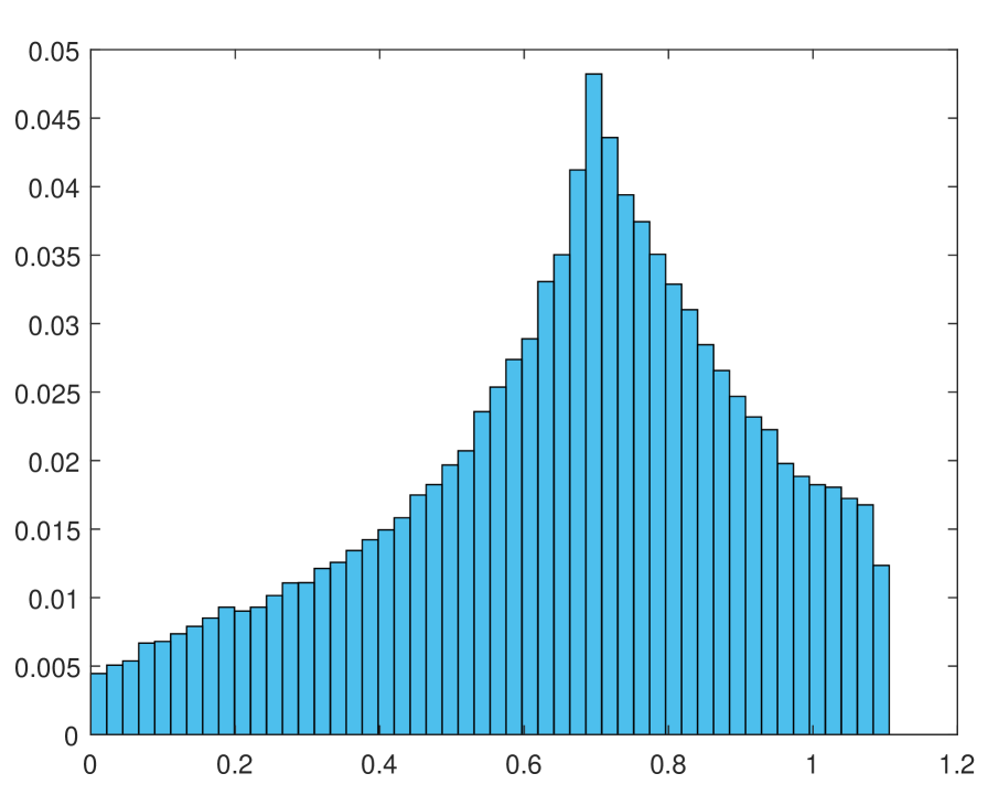
(a) prior

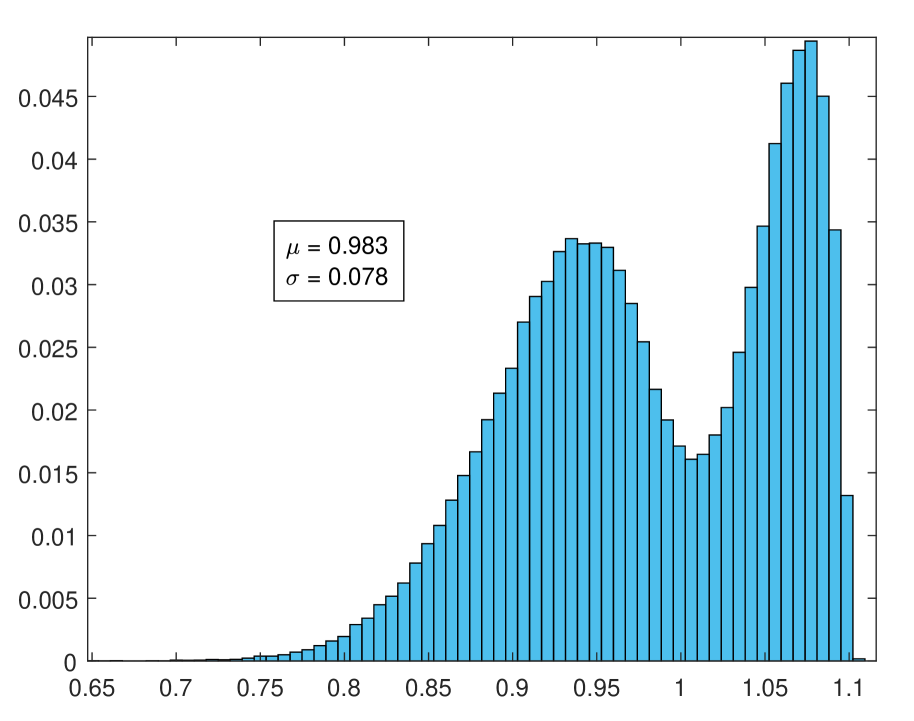
(b) $n=100$

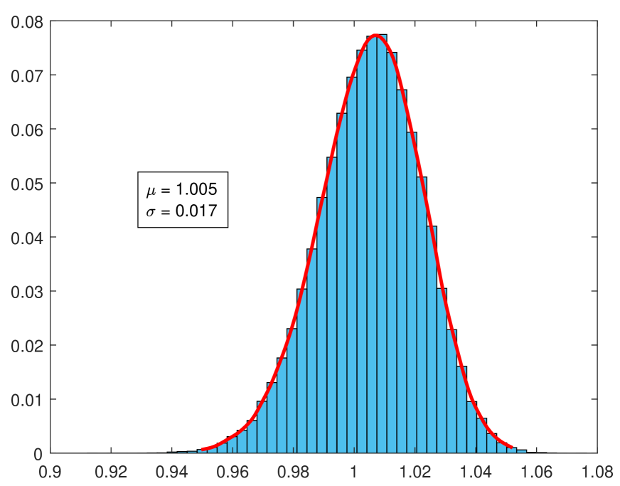
(c) $n=1000$

Figure 1: Prior $\pi(\bar{H})$ and posterior $\pi(\bar{H}|x)$ of the entropy rate $\bar{H}$ with $n=100$ and $n=1000$ observations $x$.

Figure 2 shows the performance of the BCT estimator compared with the other estimators described above, as a function of the length $n$ of the available observations $x$. For BCT we plot the posterior mean. For the plug-in we plot estimates with block-lengths $k=5,6,7$. It is easily observed that the BCT estimator outperforms all the alternatives, and converges faster and closer to the true value of $\bar{H}$.

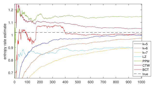
Figure 2: Entropy rate estimates for the 5th order ternary chain, as the number of observations increases.

A third order binary chain. Here, we consider $n=1000$ observations generated from an example of a third order binary chain from [2]. The underlying model is the complete binary tree of depth $3$ pruned at node $s=11$; the tree model $T$ and the parameter values $\theta=\{\theta_{s};s\in T\}$ are given in [35]. The entropy rate of this chain is $\bar{H}=0.4815$. Figure 3 shows the performance of all estimators, where BCT (using the posterior mean again) is found to have the best performance. The histogram of the BCT posterior after $n=1000$ observations is close to a Gaussian with mean $\mu=0.4806$ and standard deviation $\sigma=0.0405$.

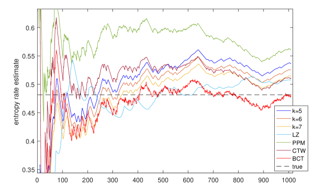
Figure 3: Entropy rate estimates for the third order binary chain, as the number of observations increases.

A bimodal posterior. We examine a simulated time series from [20], consisting of $n=1450$ observations generated from a $3$rd order chain with alphabet size $m=6$ and with the property that each $X_{n}$ depends on past observations only via $X_{n-3}$. The complete specification of the chain can be found in [20, 35]; its entropy rate is $\bar{H}=1.355$. An interesting aspect of this data set is that the model posterior is bimodal, with one mode corresponding to the empty tree (describing i.i.d. observations) and the other consisting of tree models of depth 3. As shown in Figure 4(a), the posterior of the entropy rate is also bimodal, with two approximately-Gaussian modes corresponding to the two model posterior modes.

The dominant mode is the one corresponding to models of depth 3; it has mean $\mu_{1}=1.406$, standard deviation $\sigma_{1}=0.031$, and relative weight $w_{1}=0.91$. The second mode corresponding to the empty tree has mean $\mu_{2}=1.632$, standard deviation $\sigma_{2}=0.020$, and a much smaller weight $w_{2}=1-w_{1}=0.09$. In this case, the mode of $\pi(\bar{H}|x)$ gives a more reasonable choice for a point estimate than the posterior mean. Like in the previous two examples, the BCT estimator performs better than most benchmarks.

(a) bimodal example

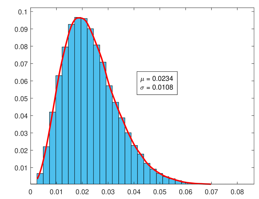
(b) spike train

Figure 4: Histograms of the posterior distribution $\pi(\bar{H}|x)$ of the entropy rate, constructed from $N=10^{5}$ i.i.d. samples.

Neural spike train. We consider $n=1000$ binary observations from a spike train recorded from a single neuron in region V4 of a monkey’s brain. The BCT posterior is shown in Figure 4(b): Its mean is $\mu=0.0234$, its standard deviation is $\sigma=0.0108$, and is skewed to the right.

This dataset is the first part of a long spike train of length $n=3,919,361$ from [15, 14]. Although there is no “true” value of the entropy rate here, for the purposes of comparison we use the estimate obtained by the naive CTW estimator (identified as the most effective method by [12] and [43]) when all $n=3,919,361$ samples are used, giving $\bar{H}=0.0241$. The resulting estimates for all five methods (with the posterior mean given for BCT) are summarised in Table I, verifying again that BCT outperforms all the other methods. For the plug-in estimator (and in all subsequent examples), we only show the best block-lengths $k$.

	“True”	BCT	CTW	PPM	LZ	$k=5$
$\widehat{H}$	0.0241	0.0234	0.0249	0.0360	0.0559	0.0204

TABLE I: Entropy rate estimates for the neural spike train.

Financial data. Here, we consider $n=2000$ observations from the financial dataset F.2 of [20]. This consists of tick-by-tick price changes of the Facebook stock price, quantised to three values: $x_{i}=0$ if the price goes down, $x_{i}=1$ if it stays the same, and $x_{i}=2$ if it goes up. The BCT entropy-rate posterior is shown in Figure 5(a): It has mean $\mu=0.921$, and standard deviation $\sigma=0.028$.

Once again, as the “true” value of the entropy rate we take the estimate produced by the naive CTW estimator on a longer sequence with $n=10^{4}$ observations, giving $\bar{H}=0.916$. The results of all five estimators are summarised in Table II, where for the BCT estimator we once again give the posterior mean, which is again found to outperform the alternatives.

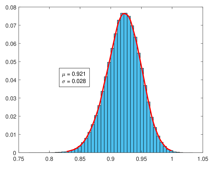
(a) financial dataset

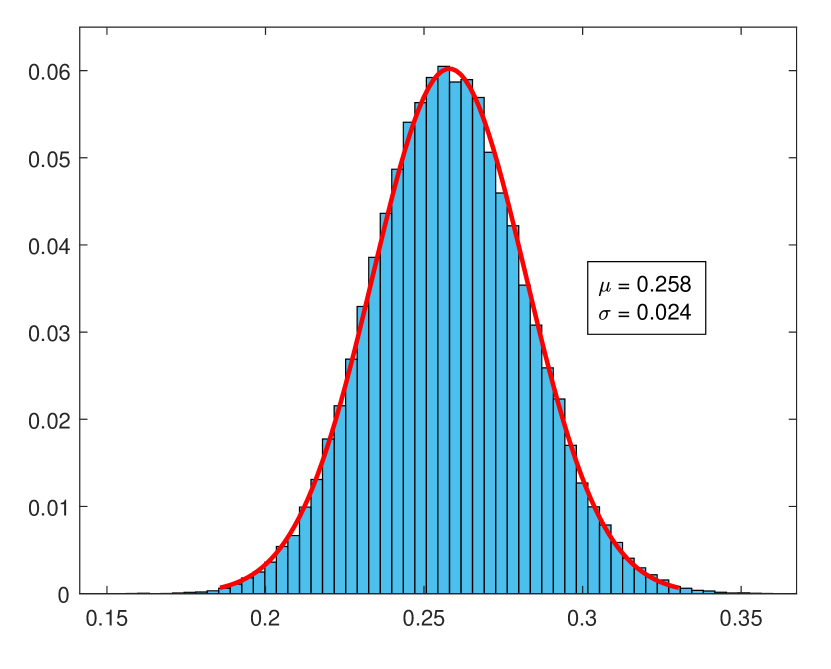
(b) pewee birdsong

Figure 5: Histograms of the posterior distribution $\pi(\bar{H}|x)$ of the entropy rate, constructed from $N=10^{5}$ i.i.d. samples.

	“True”	BCT	CTW	PPM	LZ	$k=5$	$k=6$
$\widehat{H}$	0.916	0.921	0.939	1.049	0.846	0.930	0.907

TABLE II: Entropy rate estimates for the financial data set.

Pewee birdsong. The last data set examined is a time series $x$ describing the twilight song of the wood pewee bird [10, 37]. It consists of $n=1327$ observations from an alphabet of size $m=3$. The BCT posterior is shown in Figure 5(b): It is approximately Gaussian with mean $\mu=0.258$ and standard deviation $\sigma=0.024$. The fact that the standard deviation is small suggests “confidence” in the resulting estimates, which is important because here (as in most real applications) there is no knowledge of a “true” underlying value. Table III shows all the resulting estimates; the posterior mean is shown for the BCT estimator.

	BCT	CTW	PPM	LZ	$k=5$	$k=10$	$k=15$
$\widehat{H}$	0.258	0.278	0.318	0.275	0.467	0.336	0.272

TABLE III: Entropy rate estimates for the pewee song data.

VI Concluding Remarks

The main conclusion from the results on the six data sets examined in the experimental section is that the BCT entropy estimator gives the most accurate and reliable results among the five estimators considered. In addition to the fact that the BCT point estimates typically outperform those produced by other methods, the BCT estimator is accompanied by the entire posterior distribution $\pi(\bar{H}|x)$ of the entropy rate, induced by the observations $x$. As usual, this distribution can be used to quantify the uncertainty in estimating $\bar{H}$, and it contains significantly more information than simple point estimates and their associated confidence intervals.

In closing, we note a few possible directions for future research extending this work. First, the proposed entropy estimator could be employed for the estimation of mutual information and directed information rates between processes, which come with important applications, as for example in testing for temporal causality [21]. Also, as the BCT framework has recently been extended to the setting of real-valued time series [33], it would be interesting to extend our methods for entropy estimation in the real-valued case.

References

- [1] E.W. Archer, I.M. Park, and J.W. Pillow. Bayesian entropy estimation for binary spike train data using parametric prior knowledge. Advances in neural information processing systems, 26, 2013.
- [2] A. Berchtold and A.E. Raftery. The mixture transition distribution model for high-order markov chains and non-gaussian time series. Statistical Science, 17(3):328–356, 2002.
- [3] G.S. Bhumbra and R.E.J. Dyball. Measuring spike coding in the rat supraoptic nucleus. The Journal of physiology, 555(1):281–296, 2004.
- [4] S. Bunton. On-line stochastic processes in data compression. Ph.D. thesis, University of Washington, 1996.
- [5] M. Burrows and D. Wheeler. A block-sorting lossless data compression algorithm. In Digital SRC Research Report. Citeseer, 1994.
- [6] H. Cai, S.R. Kulkarni, and S. Verdú. Universal entropy estimation via block sorting. IEEE Transactions on Information Theory, 50(7):1551–1561, 2004.
- [7] K.L. Chung. Markov chains with stationary transition probabilities. Springer-Verlag, New York, 1967.
- [8] J. Cleary and I. Witten. Data compression using adaptive coding and partial string matching. IEEE transactions on Communications, 32(4):396–402, 1984.
- [9] T.M. Cover and J.A. Thomas. Elements of information theory. J. Wiley & Sons, New York, second edition, 2012.
- [10] W. Craig. The song of the wood pewee, Myiochanes virens Linnaeus: a study of bird music. University of the State of New York, 1943.
- [11] R.E. Funderlic and C.D. Meyer. Sensitivity of the stationary distribution vector for an ergodic Markov chain. Linear Algebra and its Applications, 76:1–17, 1986.
- [12] Y. Gao, I. Kontoyiannis, and E. Bienenstock. Estimating the entropy of binary time series: Methodology, some theory and a simulation study. Entropy, 10(2):71–99, 2008.
- [13] G.H. Golub and C.D. Meyer. Using the QR factorization and group inversion to compute, differentiate, and estimate the sensitivity of stationary probabilities for Markov chains. SIAM Journal on Algebraic Discrete Methods, 7(2):273–281, 1986.
- [14] G.G. Gregoriou, S.J. Gotts, and R. Desimone. Cell-type-specific synchronization of neural activity in FEF with V4 during attention. Neuron, 73(3):581–594, 2012.
- [15] G.G. Gregoriou, S.J. Gotts, H. Zhou, and R. Desimone. High-frequency, long-range coupling between prefrontal and visual cortex during attention. Science, 324(5931):1207–1210, 2009.
- [16] A.O. Hero and O.J. Michel. Asymptotic theory of greedy approximations to minimal k-point random graphs. IEEE Transactions on Information Theory, 45(6):1921–1938, 1999.
- [17] I. Kontoyiannis. Second-order noiseless source coding theorems. IEEE Transactions on Information Theory, 43(4):1339–1341, 1997.
- [18] I. Kontoyiannis. Context-tree weighting and Bayesian Context Trees: Asymptotic and non-asymptotic justifications. arXiv preprint arXiv:2211.02676, 2022.
- [19] I. Kontoyiannis, P.H. Algoet, Y.M. Suhov, and A.J. Wyner. Nonparametric entropy estimation for stationary processes and random fields, with applications to English text. IEEE Transactions on Information Theory, 44(3):1319–1327, 1998.
- [20] I. Kontoyiannis, L. Mertzanis, A. Panotopoulou, I. Papageorgiou, and M. Skoularidou. Bayesian Context Trees: Modelling and exact inference for discrete time series. Journal of the Royal Statistical Society: Series B (Statistical Methodology), 84(4):1287–1323, 2022.
- [21] I. Kontoyiannis and M. Skoularidou. Estimating the directed information and testing for causality. IEEE Transactions on Information Theory, 62(11):6053–6067, 2016.
- [22] M. Levene and G. Loizou. Computing the entropy of user navigation in the web. International Journal of Information Technology & Decision Making, 2(03):459–476, 2003.
- [23] M. London, A. Schreibman, M. Häusser, M.E. Larkum, and I. Segev. The information efficacy of a synapse. Nature Neuroscience, 5(4):332–340, 2002.
- [24] V. Lungu, I. Papageorgiou, and I. Kontoyiannis. Bayesian change-point detection via context-tree weighting. In 2022 IEEE Information Theory Workshop (ITW), pages 125–130. IEEE, 2022.
- [25] V.M. Lungu, I. Papageorgiou, and I. Kontoyiannis. Change-point detection and segmentation of discrete data using Bayesian Context Trees. arXiv preprint arXiv:2203.04341, 2021.
- [26] T. Matsushima and S. Hirasawa. Reducing the space complexity of a Bayes coding algorithm using an expanded context tree. In 2009 IEEE International Symposium on Information Theory, pages 719–723. IEEE, 2009.
- [27] C.D. Meyer. The role of the group generalized inverse in the theory of finite Markov chains. Siam Review, 17(3):443–464, 1975.
- [28] S.P. Meyn and R.L. Tweedie. Markov chains and stochastic stability. Springer Science & Business Media, 2012.
- [29] Y. Nakahara, S. Saito, A. Kamatsuka, and T. Matsushima. Probability distribution on full rooted trees. Entropy, 24(3):328, 2022.
- [30] I. Nemenman, W. Bialek, and R.R.D.R. Van Steveninck. Entropy and information in neural spike trains: Progress on the sampling problem. Physical Review E, 69(5):056111, 2004.
- [31] L. Paninski. Estimation of entropy and mutual information. Neural Computation, 15(6):1191–1253, 2003.
- [32] L. Paninski. Estimating entropy on m bins given fewer than m samples. IEEE Transactions on Information Theory, 50(9):2200–2203, 2004.
- [33] I. Papageorgiou and I. Kontoyiannis. The Bayesian Context Trees State Space Model: Interpretable mixture models for time series. arXiv preprint arXiv:2106.03023, 2022.
- [34] I. Papageorgiou and I. Kontoyiannis. The posterior distribution of Bayesian Context-Tree models: Theory and applications. In 2022 IEEE International Symposium on Information Theory (ISIT), pages 702–707. IEEE, 2022.
- [35] I. Papageorgiou and I. Kontoyiannis. Posterior representations for Bayesian Context Trees: Sampling, estimation and convergence. Bayesian Analysis, to appear, 2023.
- [36] I. Papageorgiou, I. Kontoyiannis, L. Mertzanis, A. Panotopoulou, and M. Skoularidou. Revisiting context-tree weighting for Bayesian inference. In 2021 IEEE International Symposium on Information Theory (ISIT), pages 2906–2911, 2021.
- [37] A. Sarkar and D.B. Dunson. Bayesian nonparametric modeling of higher order Markov chains. Journal of the American Statistical Association, 111(516):1791–1803, 2016.
- [38] A.O. Schmitt and H. Herzel. Estimating the entropy of DNA sequences. Journal of theoretical biology, 188(3):369–377, 1997.
- [39] P.J. Schweitzer. Perturbation theory and finite Markov chains. Journal of Applied Probability, 5(2):401–413, 1968.
- [40] C.E. Shannon. Prediction and entropy of printed English. Bell System Technical Journal, 30(1):50–64, 1951.
- [41] S.P. Strong, R. Koberle, R.R.D.R. Van Steveninck, and W. Bialek. Entropy and information in neural spike trains. Physical Review Letters, 80(1):197, 1998.
- [42] A.W. Van der Vaart. Asymptotic statistics, volume 3. Cambridge university press, 2000.
- [43] S. Verdú. Empirical estimation of information measures: A literature guide. Entropy, 21(8):720, 2019.
- [44] F.M.J. Willems, Y.M. Shtarkov, and T.J. Tjalkens. The context-tree weighting method: basic properties. IEEE Transactions on Information Theory, 41(3):653–664, 1995.
- [45] A.D. Wyner and J. Ziv. Some asymptotic properties of the entropy of a stationary ergodic data source with applications to data compression. IEEE Transactions on Information Theory, 35(6):1250–1258, 1989.
- [46] J. Ziv and A. Lempel. A universal algorithm for sequential data compression. IEEE Transactions on Information Theory, 23(3):337–343, 1977.