compat=1.1.0, warn luatex=false
Extended Twisted Mass Collaboration
The transition form factor and the hadronic light-by-light -pole contribution to the muon from lattice QCD
Abstract
We calculate the double-virtual transition form factor from first principles using a lattice QCD simulation with quark flavors at the physical pion mass and at one lattice spacing and volume. The kinematic range covered by our calculation is complementary to the one accessible from experiment and is relevant for the -pole contribution to the hadronic light-by-light scattering in the anomalous magnetic moment of the muon. From the form factor calculation we extract the partial decay width eV and the slope parameter GeV-2. For the -pole contribution to we obtain .
I Introduction
Radiative transitions and decays of the neutral pseudoscalar mesons , and arise through the axial anomaly and are therefore a crucial probe of the nonperturbative low-energy properties of QCD. The simplest transition to two (virtual) photons, , is specified through the transition form factor (TFF) defined by the matrix element
| (1) |
where are the electromagnetic currents and are the photon momenta. The TFFs determine the partial decay widths to leading order in the fine-structure constant through
| (2) |
where is the pseudoscalar meson mass. is of particular interest, since it can be used to extract the mixing angles and provides a normalization for many other partial widths [1]. At the same time, there is a long-standing tension between its different experimental determinations through collisions on the one hand and Primakoff production on the other [2, 3, 4, 5, 6, 7, 8]. The TFFs also provide input for determining the electromagnetic interaction radius of the pseudoscalar mesons through the slope parameter
| (3) |


Moreover, the TFFs play a critical role for the leading-order hadronic light-by-light (HLbL) scattering in the anomalous magnetic moment of the muon. Recent results from the Fermilab E989 and Brookhaven E821 experiments [9, 10] indicate a tension with the consensus on the Standard Model (SM) prediction in Refs. [11, 12, 13, 14, 15, 16, 17, 18, 19, 20, 21, 22, 23, 24, 25, 26, 27, 28, 29, 30, 31]. The uncertainty of the latter is dominated by the Hadronic Vacuum Polarization and the HLbL scattering. In particular, matching the planned improvement on the experimental uncertainty by a factor of four in the SM evaluation, an improved control of the uncertainty of the HLbL contribution is mandatory, cf. Ref. [11]. The HLbL contribution can be estimated, among other approaches [32, 33, 34, 35, 36, 37, 38, 39, 40, 23], by a systematic decomposition into contributions from various intermediate states [41, 42, 43, 44]. Lattice QCD can provide ab-initio data for the required form factors and hadron scattering amplitudes within this approach. This is thus complementary to a lattice-QCD calculation of the full HLbL scattering amplitude [45, 46, 47, 48, 49, 50].
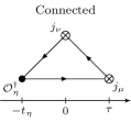
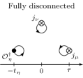
The pseudoscalar pole diagrams, depicted in Fig. 1, make the dominant contribution to the HLbL scattering amplitude, with as the key nonperturbative input. Of these diagrams, the -pole contribution has been estimated based on a dispersive framework [51, 26] and on lattice-QCD calculations of the pion TFF [52, 27, 53] while rational approximant fits to experimental TFF data have yielded an estimate of all three contributions [24]. A preliminary calculation of the - and -pole contributions using a coarse lattice was reported in Ref. [54]. Experimental results from CELLO [55], CLEO [56], and BaBar [57, 58] constrain the spacelike single-virtual in the regime , but do not provide data for or for general double-virtual kinematics. In contrast, these kinematics are the most accessible in lattice QCD and therefore provide highly relevant and important new information that is of interest for phenomenological models and various experimental efforts.
In this letter we present an ab-initio calculation of and the corresponding -pole HLbL contribution using lattice QCD simulations at a
single lattice spacing and a single volume. We employ
flavors of twisted-mass quarks [59] tuned to the
physical pion mass, physical heavy-quark masses, and maximal
twist. The latter guarantees automatic
-improvement of observables [60, 61],
which here includes , , , and .
II Methods
We apply the method introduced in Refs. [52, 27] to the case of the TFF. Details of our analysis are specified below.
II.1 Amplitude and kinematics
In particular, the TFF is related to the Euclidean -to-vacuum transition amplitude [62]
| (4) |
by
| (5) |
where counts the number of temporal indices.
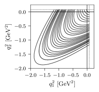
The kinematics are determined by the four-momentum of the on-shell state with energy , the four-momentum of the first current, and the momentum conservation constraint . In the lattice setup used here, it is most practical to fix and evaluate the amplitude for a variety of and . The present calculation is restricted to the rest frame, , and momenta satisfying and . Each choice of finite-volume momentum gives access to on a particular kinematical orbit, as shown in Fig. 2. Notably, the orbit lies outside the spacelike quadrant, but still falls below the nonanalytic thresholds at , allowing it to be accessed on the lattice; its proximity to makes it particularly helpful in constraining and .
II.2 Three-point function
The Euclidean amplitude in Eq. (4) is accessed by evaluating the three-point function
| (6) | ||||
For any operator with overlap onto the state, the three-point function is projected onto the physical meson at large time separation, , irrespective of mixing. Here we use , where describes the flavor structure. The validity of this choice and overlap onto the state are detailed in Appendix B. The electromagnetic currents are defined by with and [63].
Two remarks are in order concerning the definition of the three-point function using nonconserved currents. First, one can show that potential short-distance singularities are absent in Eq. (6) and that the definition admits a well defined continuum limit. The argument is given in Appendix D of Ref. [52] for Wilson fermions and, by universality, applies to Wilson twisted-mass lattice QCD as well. Second, we note that the nonconserved currents do not spoil the automatic -improvement. This is because all involved lattice quantities are constructed such that their parity covariance is ensured, i.e., they have the correct symmetry property under the twisted-mass parity transformation111Ordinary parity combined with a flavor exchange. See Ref. [64] for a comprehensive listing of symmetries of the twisted-mass action.. As a consequence, the symmetry excludes the appearance of terms in physical matrix elements, as usual for twisted-mass lattice QCD at maximal twist [60, 61], and hence guarantees automatic -improvement of the three-point function in Eq. (6).
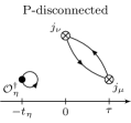
Evaluating requires the Wick contractions shown in Fig. 3. We evaluate all connected (sub-)diagrams based on point-to-all quark propagators: we build the fully connected three-point function (top-left Wick diagram in Fig. 3) from a point-to-all propagator with spin-color diluted point sources at the vertex labeled “”, with a subsequent sequential inversion through the vertex. The sequential source for this inversion is the point-to-all propagator evaluated on timeslice , and multiplied by to account for the pseudoscalar -meson interpolator. Since the meson is taken in its rest frame, no three-momentum is inserted in the sequential source.
In the P-disconnected diagram, we compute the quark-loop at from propagators based on stochastic volume sources. Straightforward (undiluted) volume sources are sufficient in this case, and we ensure that the contribution from stochastic noise is suppressed below the noise from gauge configurations.
The connected current-current two-point function sub-diagram (top-right Wick diagram in Fig. 3) we evaluate again using spin-color diluted point-to-all propagators, to allow for efficient computation with the large range of photon three-momenta employed.
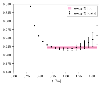
Unlike in previous lattice QCD studies of the TFF, here P-disconnected diagrams of the isospin-singlet -meson operator are nonzero. The projection onto the -meson state relies on a delicate cancellation between connected and P-disconnected diagram contributions, as shown in Fig. 5.
The amplitude is then recovered from as
| (7) |
where is the overlap factor associated with the chosen creation operator. In practice we approximate the limit by considering three fixed values of in the range . Contamination from excited states and the meson are suppressed best for the largest value of , thus we report the values for , , and from as the main result and use the remaining choices to check for excited state effects.
Statistical noise significantly hinders evaluation of for large values of . Furthermore, the finite time extent of the lattice geometry would prevent integrating in the limits even if perfectly precise data were available. To address these issues, following Refs. [52, 27, 53], we perform joint fits of the asymptotic behavior of for all to Vector Meson Dominance and Lowest Meson Dominance functional forms [65] with fit windows defined by . Details of the fitting procedure are described in Appendix. C We then integrate over as in Eq. (5) using numerical integration of the lattice data within the peak region, , and analytical integration of the fit form in the tail region, . In this work, we consider several choices of in the range . Variation between the results computed using different choices of gives a measure of the uncertainties resulting from noisy data in the tails and finite time extent effects.
II.3 Extraction of and
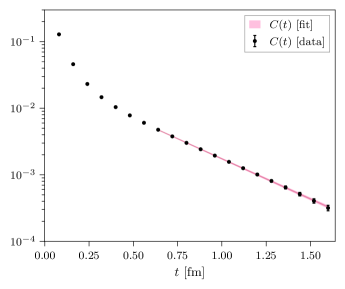
The quantities and (at rest) are extracted by fitting the two-point function of the interpolating operator selected above,
| (8) |
As the imaginary time separation is taken large, the asymptotic scaling of this function is given by a spectral decomposition,
| (9) |
where the factor of is due to the relativistic normalization of the state in the definition of . As shown in Fig. 4, we apply a two-state fit to accurately determine the scaling behavior of the two-point correlation function and its effective mass, , on the cB211.072.64 ensemble used in this work. The resulting overlap and mass parameters are determined in lattice units to be
| (10) | ||||
| (11) |
Using the lattice spacing fm determined in Ref. [63] this yields MeV in physical units. This is less than 8 permille higher than the experimental value and demonstrates the accuracy of our tuning of the valence strange-quark mass to reproduce the -meson mass. Using alternative physical quantities, such as the or , yields differences between % supporting our expectation that lattice artifacts are subleading w.r.t. the dominant statistical and other systematic errors in the TFF.
The two-point function is measured on the same gauge ensemble as the three-point function, and errors on these quantities are propagated through the calculation in a fully correlated way by using a per-bootstrap evaluation of the fitted quantities in each subsequent three-point analysis.
II.4 Extrapolation via global conformal fit
Access to the partial decay width, the slope parameter, and the -pole HLbL contribution requires an interpolation of the TFF close to the origin and an extrapolation in the quadrant of nonpositive photon virtualities. We apply the model-independent expansion in powers of conformal variables advocated in Ref. [27], termed the -expansion. Analyticity of the form factor below the two-pion thresholds at and guarantees convergence as the highest power in the expansion is taken to infinity. Moreover, the expansion is restricted to account for the known threshold scaling and contains preconditioning to more easily capture the expected asymptotic behavior as . In practice we find that the fit, consisting of six free parameters, already provides a very accurate fit to all lattice results, so we restrict to in all subsequent analyses.
To interpolate and extrapolate TFF data in the plane, we apply a global fit of the TFF data determined across all using a model-independent -expansion of order . Variation between the choice of order is included in the model averaging of all final quantities as a systematic error. The precise fit form used in this work is identical to the choice put forward in Ref. [27]. For completeness, we review this approach here.
Noting that the TFF is analytic for all virtualities (including in particular the entire spacelike quadrant, ), a conformal transformation is applied to yield the new variables
| (12) |
where and is a free parameter that determines which virtualities are mapped to the origin of the new coordinates. In the resulting coordinates, the TFF is analytic for all and can be expanded in this domain as a polynomial in , giving
| (13) |
where Bose symmetry requires that . In this expansion, the TFF is preconditioned to implement the known large-virtuality behavior already at zeroth order in the conformal expansion by including the prefactor , where is the vector-meson mass.
An order- truncation of the conformal expansion then provides a model-independent fit form to the TFF which must converge as . At finite , it is useful to further restrict the coefficients to enforce the appropriate scaling at threshold [66] by fixing the derivatives at to zero, yielding the fit function
| (14) | ||||
parameterized by fit parameters .
Finally, to optimize the rate of convergence to the TFF in the interval , the parameter is chosen to be
| (15) |
In this work, we fix . Regardless of the choice of , the expansion of the form given in Eq. (13) is guaranteed to be valid by analyticity.
We then fit the parameters of the function in Eq. (14) to our determined values of the TFF across all choices of (the orbits shown in Fig. 2 in the main text) and for choices of selected per orbit to access virtualities for which the ratios take values linearly interpolating between and along with the choices corresponding to exchanging . In total, we evaluate choices of per orbit.
Data that correspond to identical momentum and differ only in are strongly correlated, as the TFF for such choices differ only in the Laplace transform applied to identical lattice data. Data that correspond to distinct momenta are also significantly correlated due to the common underlying gauge configurations and the global fit used in the integration of . This complicates estimation of the covariance matrix required for a correlated fit. On the other hand, the model averaging procedure described in the following section is formulated to avoid needing estimates of the for fits. As such, throughout this work we choose to use uncorrelated -expansion fits to the TFF data for all quantities.
The use of an uncorrelated fit means that the associated is an unreliable measure of goodness of fit. However, the quality of the fit at order can be seen in Fig. 5 of the main text, which shows that the conformal expansion already nearly interpolates the lattice data at all orbits using only parameters. Thus only fits using orders were considered in this work.
II.5 Evaluation of
The -pole HLbL contribution has the integral representation [67, 68]
| (16) | ||||
with parameterizing the angle between the four-momenta, so that . The weight functions and are peaked such that contributions to Eq. (16) mainly come from the region [68]. Knowledge of the TFF in the regime of relatively small virtualities is thus sufficient to accurately evaluate .
Finally, we quantify systematic errors associated with the choices of tail-fit model, the parameters , and the -expansion order by the model-averaging procedure detailed in Appendix A.
III Results
Our lattice results are obtained on the flavor gauge ensemble cB211.072.64 produced by the Extended Twisted Mass Collaboration (ETMC) [69]. Key features of this ensemble are given in Table 1. The sea-quark masses for this ensemble are tuned to be isospin symmetric () and to reproduce the physical charged-pion mass and the strange- and charm-quark masses, with a lattice spacing of and a lattice size of () [69, 63]. The lattice spacing has been determined precisely in Ref. [63] using a combined analysis of meson observables across available ETMC ensembles to control finite-size effects and pion-mass dependence; in the present work, the uncertainty on the lattice-spacing determination is far below that of the lattice observables measured and these uncertainties are therefore neglected. For the valence strange quark we use the mixed action approach in Ref. [61] with a valence strange-quark doublet, whose mass is tuned such that the meson has physical mass.
| Ensemble | MDUs | [MeV] | |||
|---|---|---|---|---|---|
| cB211.072.64 |
All two-point and three-point function measurements were performed on a subset of configurations separated by two MDUs each. For the evaluation of the connected Wick contractions of the three-point function, we use point sources per configuration ( total inversions). For the current-current two-point contraction in the -disconnected diagram of the three-point function and for the connected two-point function measurements we use point sources per gauge configuration ( total inversions). Finally, we use stochastic sources per configuration ( total inversions) to evaluate pseudoscalar loops in the disconnected diagrams of both the three-point and two-point functions. Due to the twisted-mass valence action for the light- and strange-quark doublet we can use the “one-end-trick” noise reduction technique for the pseudoscalar, iso-scalar loops: In twisted-mass lattice QCD the iso-scalar loop (for either the light- or strange-quark doublet) is represented by chiral rotation as the difference of quark loops with positive and negative twisted quark mass. The latter difference is converted into a two-point function with an additional sum over the lattice four-volume. This volume average leads to enhanced suppression of stochastic noise and a more efficient stochastic estimator for the quark loop [70].
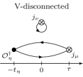
We show in Fig. 5 an example of the contributions to from the connected and P-disconnected Wick contractions on this ensemble at our largest separation, . The contributions involving strange-quark vector currents are suppressed by a factor for the connected and for the P-disconnected contribution compared to those from the light-quark vector currents. Contributions from charm-quark vector currents are expected to be even more suppressed, as are those from V-disconnected and fully disconnected diagrams (lower two diagrams in Fig. 3), based on numerical evidence from recent results for the analogous pion TFF and for the -meson TFF [27, 53, 71, 72]. At the presently achievable accuracy these contributions are hence not relevant and are not included in the analysis.
In Fig. 6 we show our results for the TFF as a function of the virtuality in the single-virtual case (top row) and in the double-virtual case (bottom row) together with our result from the -expansion fits.
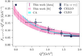
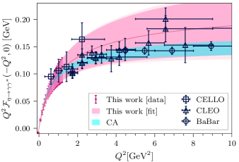
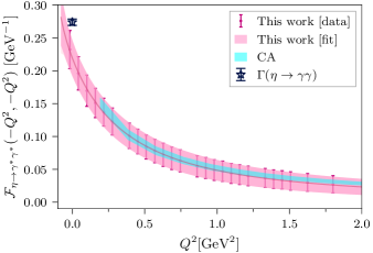
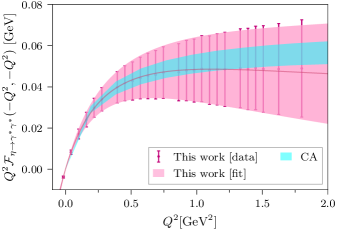
The darker inner band indicates only statistical uncertainties while the lighter outer band includes systematic uncertainties estimated from the variation of fitting choices discussed above. At all virtualities shown, the statistical errors dominate the total uncertainty. In addition to the available experimental data, we also show the Canterbury approximant (CA) result from Ref. [24]. We observe reasonable agreement between our results, the experimental data and the CA data.
From the parameterization of the momentum dependence of our TFF data we extract the decay width, slope parameter, and . As with the TFF itself, we repeat the calculation for all choices of the analysis parameters to determine systematic errors associated with tail fits of and the -expansion. A detailed breakdown is given in App. A. For the decay width the resulting systematic uncertainty stems mainly from the variation in the fits of the tails of and , while for the slope parameter and the HLbL pole contribution it is mainly due to the conformal fit. The total error, however, is always dominated by the statistical uncertainties. We also observe a mild systematic dependence on , as detailed below, which points to the fact that excited-state and possibly -meson contributions to the transition amplitude are not completely eliminated at the smaller values of . We conservatively quote results obtained at our largest value of for which the statistical uncertainty is largest and covers the results at the smaller values.
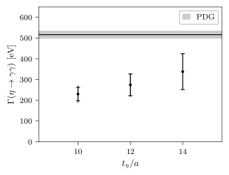
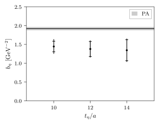
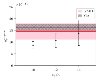
In Fig. 7 we show the dependence of the partial decay width , the slope parameter , and the -pole contribution on the choice of which denotes the imaginary time location of the creation operator for the meson, to be compared with imaginary time coordinates of the currents and . The outer error bar denotes the total error, while the inner one shows the statistical error only. It is clear that the total error is dominated by the statistical one in all cases and for all considered in this calculation. For all three quantities we observe a mild systematic trend with growing which may be an indication that excited state and -meson contributions to the transition amplitude, and hence to the quantities shown here, may still be present at the smaller values of . Since we are interested in the limit we conservatively quote the results for the largest available for which the statistical error is largest and covers the results at the smaller values of .
For the leading-order decay width we obtain
| (17) |
in comparison to the experimental average [1, 3, 4, 5, 6, 7]. For the slope parameter we find
| (18) |
to be compared with GeV-2 from a Padé approximant fit to the experimental results [73] and GeV-2 from a dispersive calculation [74]. Finally, we use the parameterization of our TFF data to perform the integration in Eq. (16) and obtain
| (19) |
in comparison to a Canterbury approximant fit to experimental results yielding [24], the VMD model value [68], and estimates [75] and [76] based on the Dyson-Schwinger equations.
We emphasize that our results are obtained at a fixed lattice spacing and a fixed volume.
The present estimates therefore exclude systematic errors associated
with finite-volume effects and lattice artifacts.
The latter are expected to be of
with the lattice discretization used here, while the former are
expected to be suppressed by with .
They are hence expected to be subleading w.r.t. to the dominating statistical and
other systematic errors in the TFF. Lattice artifacts contribute through the bare TFFs, the vector-current renormalization factors (except in )
and through the setting of the lattice scale required to convert to lattice units.
Both and the lattice scale are determined
independently of the quantities considered here [63, 69].
A quantitative estimate of the lattice artifacts present in
can therefore be obtained by considering the
scheme of fixing the renormalization by the physical decay width instead of the hadronic scheme.
This gives
,
which differs from in Eq. (19) by and is of similar size as our total error.
IV Conclusions and outlook
The results of our lattice QCD calculation of the transition form factor at physical pion mass have a precision comparable to experimental results in the range where both are available, and demonstrate nice agreement, cf. Fig. 6. Our results provide single-virtual data at lower photon virtuality than currently accessible by experiments. This includes the region around zero virtuality necessary to study the decay width and slope parameter. The results for these quantities in Eqs. (17) and (18) undershoot the experimental (and for also theoretical) results by 1.5–2.0 standard deviations.
Our lattice computation also provides TFF data for double-virtual (space-like) photon kinematics, which is difficult to access by experiment. We have made use of this advantage and calculated the -pole contribution to the anomalous magnetic moment of the muon, . Our result confirms the currently available data-driven Canterbury approximant estimate [24] and the theoretical model estimates [68, 75, 76], but does not yet reach the same precision. Nevertheless, it provides important independent support of these estimates. The main shortcoming of our calculation is the use of a single lattice spacing, which will be removed in the future by computations with ETMC gauge ensembles on finer lattices [69, 77].
Note added: While our paper was under review a comprehensive study of the pseudoscalar TFFs and their contribution to has appeared, including results for the meson [71].
Acknowledgements.
We thank Martin Hoferichter, Simon Holz, and Bastian Kubis for helpful discussions. We are also grateful to the authors of Ref. [24] for sharing form factor data produced in their work. This work is supported in part by the Sino-German collaborative research center CRC 110 and the Swiss National Science Foundation (SNSF) through grant No. 200021_175761, 200020_208222, and 200020_200424. We gratefully acknowledge computing time granted on Piz Daint at Centro Svizzero di Calcolo Scientifico (CSCS) via the projects s849, s982, s1045 and s133. Some figures were produced using matplotlib [78].Appendix A Error estimation and model averaging
All statistical errors reported in this work are given as confidence intervals derived from bootstrap resamplings of the ensemble of configurations. We find virtually no autocorrelation between the relevant primary data taken on a subset of configurations constituting the ensemble, and the bootstrap bin size is therefore fixed to .
| [] | [] | ||
| Tail model vs data cut () | 0.22 | 10.1 | 0.020 |
| Tail fit windows (, ) | 0.18 | 6.5 | 0.009 |
| Fit model (VMD vs. LMD) | 0.31 | 11.6 | 0.034 |
| Conformal fit order () | 1.44 | 1.8 | 0.123 |
| Total systematic | 1.53 | 17.2 | 0.135 |
| Statistical | 5.24 | 86.7 | 0.279 |
| Total | 5.46 | 88.4 | 0.310 |
During our analysis, we make several choices corresponding to fits of the large- tails of the amplitude and of the finite-volume TFF orbits. In particular, the following analysis parameters are varied:
-
1.
The choice between using the Vector Meson Dominance (VMD) or Lowest Meson Dominance (LMD) model to the fit the tail behavior;
-
2.
The window , determining which regions of the amplitude are used as inputs to fit the asymptotic tail behavior;
-
3.
The integration cutoff , distinguishing the region in which the lattice data is integrated from the region in which the analytical tail model is integrated; and
-
4.
The order of the conformal expansion used to fit the TFFs.
The variation of our estimates with these model choices gives estimates of the systematic errors associated with these steps. We apply the approach of Refs. [79, 80] to construct cumulative distribution functions (CDFs) of all final quantities with various subsets of models and with two choices of rescaling parameter applied to the systematic error. The various total error estimates, given by the difference between the 16th and 84th percentiles of the CDF in each case, allow an extraction and decomposition of the total uncertainty into statistical, total systematic, and various individual sources.
In this approach, weights must be assigned to each model included in the CDF. Weights based on the Akaike Information Criterion [81] derived from values of each fit have been employed in previous work. For the tail of the amplitude, we perform a fit to values of over sequential choices of and across all momentum orbits. For the -expansion, we perform a fit to values of across all orbits at several fixed choices of the ratio . As discussed in the previous section, this input data is highly correlated, and determining the correlated therefore requires a very precise estimate of nearly degenerate covariance matrices of both the tail fits and -expansion fits. Even for fits to small windows and few choices of orbits, we found estimates of the values to be inaccurate and unstable in our preliminary investigations. Instead, in this work we derive all results from much more stable uncorrelated fits. For the model averaging, we then make the conservative choice to use a uniform weighting of all possible models in the CDF method. This can be expected to overestimate the systematic error associated with model variation.
The decomposition of uncertainties is detailed in Table 2 for all three final physical quantities studied in this work. Due to correlations between the total error estimates in each case, the decomposition does not simply add in quadrature, but nevertheless gives an estimate of which components of the error dominate the error budget. Unsurprisingly, the dominant sources of systematic errors vary depending on the observable considered. For the -pole contribution to the HLbL, the biggest source of systematic error is the conformal fit used to extrapolate the TFF from the low-virtuality orbits accessible on the lattice to the full plane of spacelike . This indicates that, despite the important contributions to from low virtualities, the large uncertainties in the nearly unconstrained higher virtualities can still affect the estimate of from lattice data alone. Incorporating some information about asymptotic scaling of the TFF at large virtualities is therefore an interesting prospect for future work. The other two quantities, and are directly related to the behavior of the TFF at . In the case of , the choices used to fit the tails of the amplitude dominate the systematic errors, while for the systematic uncertainties are still set by the conformal expansion fit. Nonetheless, we find that the uncertainties in all three quantities are almost entirely given by the statistical error, which always far outweighs the systematic errors.
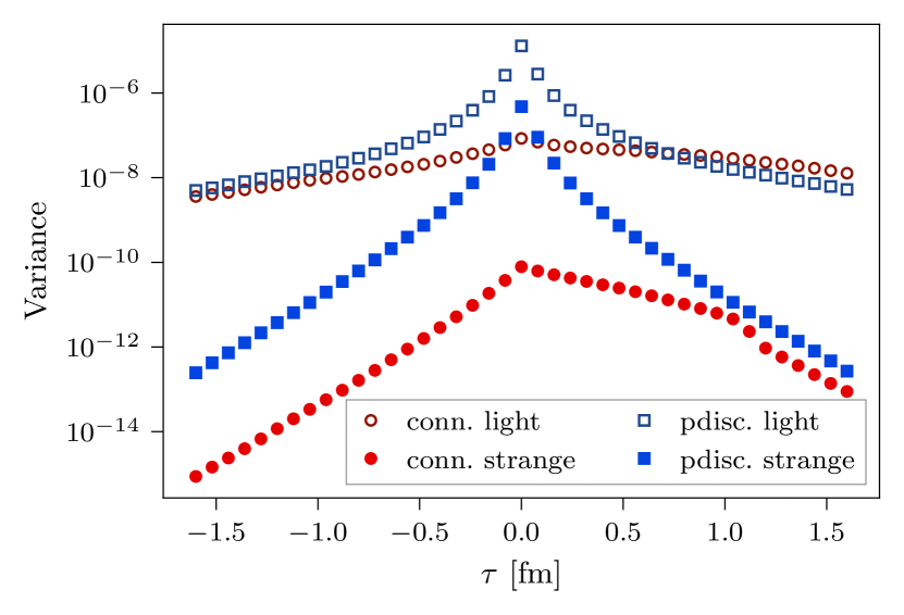
The global fit used in the integration of prevents decomposing the precise contribution of statistical errors to the final values of , , and . However, one can consider the relative contributions of various Wick contractions to itself to qualitatively understand the dominant source of statistical error. This is shown for the example of the orbit in Fig. 8, which can be compared against the plot of these same contributions in Fig. 4 of the main text. Correlations of the errors prevent interpreting the contributions as a direct decomposition of the total error, however one can still identify the Wick contractions dominating the error for various values of . In particular, at values of , the P-disconnected diagrams dominate the variance, while for the connected light diagram also makes a notable contribution.
Appendix B Interpolation of the state
The -meson state is the lowest-lying eigenstate of the twisted-mass lattice Hamiltonian in the channel with quantum numbers . The exact interpolating field to project onto the eigenstate in the lattice calculation is unknown. However, it is sufficient that it can be written as a linear combination of the quark-model octet- and singlet-pseudoscalar operators
| (20) | ||||
where the ellipsis denotes further linearly independent operators. Using the octet operator
| (21) |
as the interpolating operator means that the projection is imperfect, i.e., the creation operator will produce a tower of Hamiltonian eigenstates from the vacuum,
| (22) |
with increasing mass or energy and with , . Nevertheless, the -meson state is the unique ground state of lowest mass, and propagation in Euclidean time systematically suppresses the contribution of the -meson and excited states lying higher in the spectrum. This suppression scales exponentially as , in terms of the Euclidean time evolution and the relative energy gap between the mass of the higher state and . This applies to all two- and three-point correlation functions used in this work. Thus for sufficiently long Euclidean time propagation, the projection onto the -meson state is achieved by our choice of as the creation operator for the two-point and three-point functions.
Appendix C VMD and LMD fits to the amplitude
As discussed in Sec. II.2, we perform global fits to the amplitudes across all vector current momenta and use the resulting functional forms instead of data when integrating Eq. (5) at large . Here we detail the functional forms used for the fits, which are inspired by the Vector Meson Dominance (VMD) and Lowest Meson Dominance (LMD) models [82, 83].
The transition form factor in the VMD and LMD models are respectively given by
| (23) |
and
| (24) |
where phenomenology suggests the particular choice (the mass of the meson) and choices of and to respectively match the triangle anomaly, which determines to leading order [84, 85], and the short distance doubly virtual behavior [86, 87, 88, 89]. Note that the VMD model is simply a special case of the LMD model with fixed to zero. For fits to the lattice amplitude data, these parameters will be taken as free parameters of the fitting function.
Inverting the relation in Eq. (5) between the TFF and amplitude in the rest frame of the meson results in a functional form for the amplitude using the LMD model (or by fixing the VMD model),
| (25) | ||||
where
| (26) | ||||
References
- [1] Particle Data Group Collaboration, R. L. Workman and Others, PTEP 2022, 083C01 (2022).
- [2] L. Gan, B. Kubis, E. Passemar and S. Tulin, Phys. Rept. 945, 1 (2022), arXiv:2007.00664 [hep-ph].
- [3] JADE Collaboration, W. Bartel et al., Phys. Lett. B 158, 511 (1985).
- [4] Crystal Ball Collaboration, D. Williams et al., Phys. Rev. D 38, 1365 (1988).
- [5] N. A. Roe et al., Phys. Rev. D 41, 17 (1990).
- [6] S. E. Baru et al., Z. Phys. C 48, 581 (1990).
- [7] KLOE-2 Collaboration, D. Babusci et al., JHEP 01, 119 (2013), arXiv:1211.1845 [hep-ex].
- [8] A. Browman et al., Phys. Rev. Lett. 32, 1067 (1974).
- [9] Muon g-2 Collaboration, B. Abi et al., Phys. Rev. Lett. 126, 141801 (2021), arXiv:2104.03281 [hep-ex].
- [10] Muon g-2 Collaboration, G. W. Bennett et al., Phys. Rev. D 73, 072003 (2006), arXiv:hep-ex/0602035.
- [11] T. Aoyama et al., Phys. Rept. 887, 1 (2020), arXiv:2006.04822 [hep-ph].
- [12] T. Aoyama, M. Hayakawa, T. Kinoshita and M. Nio, Phys. Rev. Lett. 109, 111808 (2012), arXiv:1205.5370 [hep-ph].
- [13] T. Aoyama, T. Kinoshita and M. Nio, Atoms 7, 28 (2019).
- [14] A. Czarnecki, W. J. Marciano and A. Vainshtein, Phys. Rev. D 67, 073006 (2003), arXiv:hep-ph/0212229, [Erratum: Phys.Rev.D 73, 119901 (2006)].
- [15] C. Gnendiger, D. Stöckinger and H. Stöckinger-Kim, Phys. Rev. D 88, 053005 (2013), arXiv:1306.5546 [hep-ph].
- [16] M. Davier, A. Hoecker, B. Malaescu and Z. Zhang, Eur. Phys. J. C 77, 827 (2017), arXiv:1706.09436 [hep-ph].
- [17] A. Keshavarzi, D. Nomura and T. Teubner, Phys. Rev. D 97, 114025 (2018), arXiv:1802.02995 [hep-ph].
- [18] G. Colangelo, M. Hoferichter and P. Stoffer, JHEP 02, 006 (2019), arXiv:1810.00007 [hep-ph].
- [19] M. Hoferichter, B.-L. Hoid and B. Kubis, JHEP 08, 137 (2019), arXiv:1907.01556 [hep-ph].
- [20] M. Davier, A. Hoecker, B. Malaescu and Z. Zhang, Eur. Phys. J. C 80, 241 (2020), arXiv:1908.00921 [hep-ph], [Erratum: Eur.Phys.J.C 80, 410 (2020)].
- [21] A. Keshavarzi, D. Nomura and T. Teubner, Phys. Rev. D 101, 014029 (2020), arXiv:1911.00367 [hep-ph].
- [22] A. Kurz, T. Liu, P. Marquard and M. Steinhauser, Phys. Lett. B 734, 144 (2014), arXiv:1403.6400 [hep-ph].
- [23] K. Melnikov and A. Vainshtein, Phys. Rev. D 70, 113006 (2004), arXiv:hep-ph/0312226.
- [24] P. Masjuan and P. Sanchez-Puertas, Phys. Rev. D 95, 054026 (2017), arXiv:1701.05829 [hep-ph].
- [25] G. Colangelo, M. Hoferichter, M. Procura and P. Stoffer, JHEP 04, 161 (2017), arXiv:1702.07347 [hep-ph].
- [26] M. Hoferichter, B.-L. Hoid, B. Kubis, S. Leupold and S. P. Schneider, JHEP 10, 141 (2018), arXiv:1808.04823 [hep-ph].
- [27] A. Gérardin, H. B. Meyer and A. Nyffeler, Phys. Rev. D 100, 034520 (2019), arXiv:1903.09471 [hep-lat].
- [28] J. Bijnens, N. Hermansson-Truedsson and A. Rodríguez-Sánchez, Phys. Lett. B 798, 134994 (2019), arXiv:1908.03331 [hep-ph].
- [29] G. Colangelo, F. Hagelstein, M. Hoferichter, L. Laub and P. Stoffer, JHEP 03, 101 (2020), arXiv:1910.13432 [hep-ph].
- [30] T. Blum et al., Phys. Rev. Lett. 124, 132002 (2020), arXiv:1911.08123 [hep-lat].
- [31] G. Colangelo, M. Hoferichter, A. Nyffeler, M. Passera and P. Stoffer, Phys. Lett. B 735, 90 (2014), arXiv:1403.7512 [hep-ph].
- [32] T. Kinoshita, B. Nizic and Y. Okamoto, Phys. Rev. D 31, 2108 (1985).
- [33] E. de Rafael, Phys. Lett. B 322, 239 (1994), arXiv:hep-ph/9311316.
- [34] J. Bijnens, E. Pallante and J. Prades, Phys. Rev. Lett. 75, 1447 (1995), arXiv:hep-ph/9505251, [Erratum: Phys.Rev.Lett. 75, 3781 (1995)].
- [35] J. Bijnens, E. Pallante and J. Prades, Nucl. Phys. B 474, 379 (1996), arXiv:hep-ph/9511388.
- [36] J. Bijnens, E. Pallante and J. Prades, Nucl. Phys. B 626, 410 (2002), arXiv:hep-ph/0112255.
- [37] M. Hayakawa, T. Kinoshita and A. I. Sanda, Phys. Rev. Lett. 75, 790 (1995), arXiv:hep-ph/9503463.
- [38] M. Hayakawa, T. Kinoshita and A. I. Sanda, Phys. Rev. D 54, 3137 (1996), arXiv:hep-ph/9601310.
- [39] M. Hayakawa and T. Kinoshita, Phys. Rev. D 57, 465 (1998), arXiv:hep-ph/9708227, [Erratum: Phys.Rev.D 66, 019902 (2002)].
- [40] M. Knecht and A. Nyffeler, Phys. Rev. D 65, 073034 (2002), arXiv:hep-ph/0111058.
- [41] G. Colangelo, M. Hoferichter, M. Procura and P. Stoffer, JHEP 09, 091 (2014), arXiv:1402.7081 [hep-ph].
- [42] G. Colangelo, M. Hoferichter, B. Kubis, M. Procura and P. Stoffer, Phys. Lett. B 738, 6 (2014), arXiv:1408.2517 [hep-ph].
- [43] G. Colangelo, M. Hoferichter, M. Procura and P. Stoffer, JHEP 09, 074 (2015), arXiv:1506.01386 [hep-ph].
- [44] V. Pauk and M. Vanderhaeghen, Phys. Rev. D 90, 113012 (2014), arXiv:1409.0819 [hep-ph].
- [45] T. Blum, S. Chowdhury, M. Hayakawa and T. Izubuchi, Phys. Rev. Lett. 114, 012001 (2015), arXiv:1407.2923 [hep-lat].
- [46] T. Blum et al., Phys. Rev. D 93, 014503 (2016), arXiv:1510.07100 [hep-lat].
- [47] T. Blum et al., Phys. Rev. Lett. 118, 022005 (2017), arXiv:1610.04603 [hep-lat].
- [48] T. Blum et al., Phys. Rev. D 96, 034515 (2017), arXiv:1705.01067 [hep-lat].
- [49] E.-H. Chao et al., Eur. Phys. J. C 81, 651 (2021), arXiv:2104.02632 [hep-lat].
- [50] E.-H. Chao, R. J. Hudspith, A. Gérardin, J. R. Green and H. B. Meyer, Eur. Phys. J. C 82, 664 (2022), arXiv:2204.08844 [hep-lat].
- [51] M. Hoferichter, B.-L. Hoid, B. Kubis, S. Leupold and S. P. Schneider, Phys. Rev. Lett. 121, 112002 (2018), arXiv:1805.01471 [hep-ph].
- [52] A. Gérardin, H. B. Meyer and A. Nyffeler, Phys. Rev. D 94, 074507 (2016), arXiv:1607.08174 [hep-lat].
- [53] S. A. Burri et al., PoS LATTICE2021, 519 (2022), arXiv:2112.03586 [hep-lat].
- [54] BMW Collaboration, A. Gérardin, J. N. Guenther, L. Varnhorst and W. E. A. Verplanke, PoS LATTICE2022, 332 (2022), arXiv:2211.04159 [hep-lat].
- [55] CELLO Collaboration, H. J. Behrend et al., Z. Phys. C 49, 401 (1991).
- [56] CLEO Collaboration, J. Gronberg et al., Phys. Rev. D 57, 33 (1998), arXiv:hep-ex/9707031.
- [57] BaBar Collaboration, B. Aubert et al., Phys. Rev. D 80, 052002 (2009), arXiv:0905.4778 [hep-ex].
- [58] BaBar Collaboration, P. del Amo Sanchez et al., Phys. Rev. D 84, 052001 (2011), arXiv:1101.1142 [hep-ex].
- [59] Alpha Collaboration, R. Frezzotti, P. A. Grassi, S. Sint and P. Weisz, JHEP 08, 058 (2001), arXiv:hep-lat/0101001.
- [60] R. Frezzotti and G. C. Rossi, JHEP 08, 007 (2004), arXiv:hep-lat/0306014.
- [61] R. Frezzotti and G. C. Rossi, JHEP 10, 070 (2004), arXiv:hep-lat/0407002.
- [62] X.-d. Ji and C.-w. Jung, Phys. Rev. Lett. 86, 208 (2001), arXiv:hep-lat/0101014.
- [63] ETM Collaboration, C. Alexandrou et al., Phys. Rev. D 107, 074506 (2023), arXiv:2206.15084 [hep-lat].
- [64] A. Shindler, Phys. Rept. 461, 37 (2008), arXiv:0707.4093 [hep-lat].
- [65] V. L. Chernyak and S. I. Eidelman, Prog. Part. Nucl. Phys. 80, 1 (2015), arXiv:1409.3348 [hep-ph].
- [66] C. Bourrely, I. Caprini and L. Lellouch, Phys. Rev. D 79, 013008 (2009), arXiv:0807.2722 [hep-ph], [Erratum: Phys.Rev.D 82, 099902 (2010)].
- [67] F. Jegerlehner and A. Nyffeler, Phys. Rept. 477, 1 (2009), arXiv:0902.3360 [hep-ph].
- [68] A. Nyffeler, Phys. Rev. D 94, 053006 (2016), arXiv:1602.03398 [hep-ph].
- [69] ETM Collaboration, C. Alexandrou et al., Phys. Rev. D 104, 074515 (2021), arXiv:2104.13408 [hep-lat].
- [70] C. Alexandrou et al., Comput. Phys. Commun. 185, 1370 (2014), arXiv:1309.2256 [hep-lat].
- [71] A. Gérardin et al., arXiv:2305.04570 [hep-lat].
- [72] C. Alexandrou et al., arXiv:2308.12458 [hep-lat].
- [73] R. Escribano, P. Masjuan and P. Sanchez-Puertas, Eur. Phys. J. C 75, 414 (2015), arXiv:1504.07742 [hep-ph].
- [74] B. Kubis and J. Plenter, Eur. Phys. J. C 75, 283 (2015), arXiv:1504.02588 [hep-ph].
- [75] G. Eichmann, C. S. Fischer, E. Weil and R. Williams, Phys. Lett. B 797, 134855 (2019), arXiv:1903.10844 [hep-ph], [Erratum: Phys.Lett.B 799, 135029 (2019)].
- [76] K. Raya, A. Bashir and P. Roig, Phys. Rev. D 101, 074021 (2020), arXiv:1910.05960 [hep-ph].
- [77] ETM Collaboration, C. Alexandrou et al., Phys. Rev. D 104, 074520 (2021), arXiv:2104.06747 [hep-lat].
- [78] J. D. Hunter, Computing in Science & Engineering 9, 90 (2007).
- [79] S. Borsanyi et al., Science 347, 1452 (2015).
- [80] S. Borsanyi et al., Nature 593, 51 (2021), arXiv:2002.12347.
- [81] H. Akaike, Annals of the Institute of Statistical Mathematics 30, 9 (1978).
- [82] B. Moussallam, Phys. Rev. D 51, 4939 (1995), arXiv:hep-ph/9407402.
- [83] M. Knecht, S. Peris, M. Perrottet and E. de Rafael, Phys. Rev. Lett. 83, 5230 (1999), arXiv:hep-ph/9908283.
- [84] S. L. Adler, Phys. Rev. 177, 2426 (1969).
- [85] J. S. Bell and R. Jackiw, Nuovo Cim. A 60, 47 (1969).
- [86] G. P. Lepage and S. J. Brodsky, Phys. Lett. B 87, 359 (1979).
- [87] G. P. Lepage and S. J. Brodsky, Phys. Rev. D 22, 2157 (1980).
- [88] V. A. Nesterenko and A. V. Radyushkin, Sov. J. Nucl. Phys. 38, 284 (1983).
- [89] V. A. Novikov, M. A. Shifman, A. I. Vainshtein, M. B. Voloshin and V. I. Zakharov, Nucl. Phys. B 237, 525 (1984).