Quantum field corrections to the equation of state of freely streaming matter in the Friedman-Lemaître-Robertson-Walker space-time

Abstract

We calculate the energy density and pressure of a scalar field after its decoupling from a thermal bath in the spatially flat Friedman-Lemaître-Robertson-Walker space-time, within the framework of quantum statistical mechanics. By using the density operator determined by the condition of local thermodynamic equilibrium, we calculate the mean value of the stress-energy tensor of a real scalar field by subtracting the vacuum expectation value at the time of the decoupling. The obtained expressions of energy density and pressure involve corrections with respect to the classical free-streaming solution of the relativistic Boltzmann equation, which may become relevant even at long times.

I Introduction

A key ingredient in cosmology is the equation of state of matter, i.e. the relation between energy density $\varepsilon$ and the pressure $p$. They are the only two independent scalar quantities appearing in the stress-energy tensor that are allowed by the symmetries of the Friedman-Lemaître-Robertson-Walker (FLRW) metric. In the comoving cosmological coordinates this reads:

$${\rm d}s^{2}={\rm d}t^{2}-a(t)^{2}\left(\frac{{\rm d}r^{2}}{1-Kr^{2}}+r^{2}{\rm d}\Omega^{2}\right)$$ (1)

where $a(t)$ is the scale factor and $K=0,\pm 1$. Indeed, the isotropy and homogeneity of the Universe, encoded in the metric (1), dictates that the rank 2 symmetric stress-energy tensor can only be of the perfect fluid form:

$$T^{\mu\nu}=(\varepsilon+p)\,u^{\mu}u^{\nu}-pg^{\mu\nu}$$ (2)

where $u^{\mu}=(1,{\bf 0})$.

The equation of state of ordinary (or dark) matter is usually inferred by imposing thermodynamic equilibrium relations. Strictly speaking, thermodynamic equilibrium is possible only in stationary space-times, endowed with a global Killing time-like vector. Indeed, thermal field theory in curved stationary space-times has been the subject of several studies in literature dowker1 ; dowker2 ; critchley ; miele . However, in an expanding Universe described by the FLRW metric (1) only local thermodynamic equilibrium can be defined. Local equilibrium applies as long as matter is coupled within the cosmological plasma; when matter, in the form of a specific quantum field, decouples because the expansion rate exceeds the reaction rate kolbturner particle spectra get frozen thereafter. The freeze-out process is usually studied by means of the classical relativistic kinetic theory, specifically the relativistic Boltzmann equation kremer . After freeze-out, the classical phase space distribution function $f(x,k)$ is the so-called free-streaming solution of the Boltzmann equation and the relation between stress-energy tensor and distribution function reads piattella :

$$T^{\mu\nu}=\int{\rm d}k_{1}{\rm d}k_{2}{\rm d}k_{3}\;\frac{k^{\mu}k^{\nu}}{k^{0}\sqrt{-g}}f(x,k)$$

where $k$ is the four-momentum of the particle. Since the covariant components $k_{\mu}$ are conserved in the cosmological free fall, the solution of the relativistic Boltzmann equation is simply:

$$f(t,x^{1},x^{2},x^{3},k_{\mu})=f_{0}(t_{0},x^{1},x^{2},x^{3},k_{\mu})$$

where $f_{0}$ is the distribution function at the time $t_{0}$. Thus, in the approximation of a sudden freeze-out, that is of an instantaneous transition from local thermodynamic equilibrium to a non interacting system, the energy density and pressure of, e.g., freely streaming neutral spinless particles read:

$$\begin{split}\varepsilon(t)&=\frac{1}{(2\pi)^{3}a^{4}(t)}\int{\rm d}^{3}{\rm k}\;\sqrt{{\rm k}^{2}+m^{2}a^{2}(t)}\frac{1}{{\rm e}^{\sqrt{{\rm k}^{2}+m^{2}}/T(t_{0})}-1}\\ p(t)&=\frac{1}{3(2\pi)^{3}a^{4}(t)}\int{\rm d}^{3}{\rm k}\;\frac{{\rm k}^{2}}{\sqrt{{\rm k}^{2}+m^{2}a^{2}(t)}}\frac{1}{{\rm e}^{\sqrt{{\rm k}^{2}+m^{2}}/T(t_{0})}-1}\end{split}$$ (3)

where ${\bf k}$ are the space covariant components, in the metric (1), of the particle four-momentum vector (which are conserved in the free-streaming), and ${\rm k}^{2}=k_{x}^{2}+k_{y}^{2}+k_{z}^{2}$; $T(t_{0})$ is the temperature at the decoupling, or freeze-out in this approximation, and the scale factor $a(t_{0})$ at the freeze-out time $t_{0}$ is set to be 1, which will be henceforth assumed.

In this work, we will show that a proper quantum statistical handling implies corrections to the energy density and pressure (3) expressions of the free-streaming solution for a sudden freeze-out which, in principle, can become relevant also at late times. We will show that such corrections arise from the interplay of quantum statistical mechanics and the evolution of free fields in a curved spacetime. If such corrections were relevant at macroscopic times, they could have an impact on the evolution of the Universe as a whole as well as on the structure formation because they imply a quantum correction to statistical fluctuations of energy density.

The existence of corrections to the classical expressions from relativistic kinetic theory in the cosmological metric was pointed out in refs. fonarev1 ; fonarev2 ; full expressions of energy density and pressure at global thermodynamic equilibrium in special curved space-times have been obtained, e.g. for the anti-De Sitter space-time allen ; ambrus . Herein, we derive a general expression of energy density and pressure for the free scalar field in the spatially flat FLRW universe, where only a local thermodynamic equilibrium can be defined, showing that there are non-trivial corrections to the (3). The obtained expressions depend on the solutions of the Klein-Gordon equation in the FLRW metric, whose analytic form essentially depends on the function $a(t)$. We will not work out the solutions for specific scale factor functions, which is a considerable problem on its own, deferring it to a paper dedicated to this topic becarose2 .

Notation

In this paper we use the natural units, with $\hbar=c=K=1$. The Minkowskian metric tensor $\eta$ is ${\rm diag}(1,-1,-1,-1)$; for the Levi-Civita symbol we use the convention $\epsilon^{0123}=1$.
We will use the relativistic notation with repeated indices assumed to be saturated. Operators in Hilbert space will be denoted by a wide upper hat, e.g. $\widehat{H}$. Sometimes, scalar products of four-vectors such as $V_{\mu}U^{\mu}$ will be denoted with a dot, i.e. $V\cdot U$. The Riemann tensor is defined as $R^{\mu}_{\;\;\rho\lambda\nu}=\partial_{\lambda}\Gamma^{\mu}_{\rho\nu}-\partial_{\nu}\Gamma^{\mu}_{\rho\lambda}+\Gamma^{\mu}_{\lambda\sigma}\Gamma^{\sigma}_{\rho\nu}-\Gamma^{\mu}_{\nu\sigma}\Gamma^{\sigma}_{\rho\lambda}$

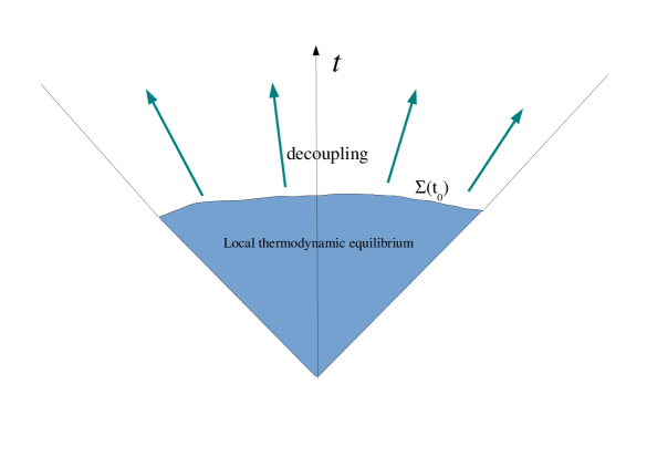
Figure 1: Schematic illustration of the evolution of a matter field as a function of cosmological time in the Friedman-Lemaître-Robertson-Walker universe. Until some time $t_{0}$ and the corresponding space-like hypersurface $\Sigma(t_{0})$, the field is coupled to the cosmological plasma, thereafter it decouples and evolves freely. We take the approximation of an instantaneous cease of interactions, implying that decoupling - defined as the time where the expansion rate overcomes the interaction rate - coincides with the freeze-out, defined as the time when interactions cease and the field becomes effectively free.

II Local equilibrium and the expectation value of the stress-energy tensor

The expectation value of the stress-energy tensor in curved space-time is a key ingredient for the solution of the semi-classical Einstein equation:

$$R_{\mu\nu}-\frac{1}{2}Rg_{\mu\nu}=8\pi G\langle{\widehat{T}}_{\mu\nu}\rangle_{\rm ren}$$ (4)

This depends, in the first place, on the quantum state of the Universe, which is in principle unknown. The calculation of a renormalized value of ${\widehat{T}}^{\mu\nu}$ in an arbitrary pure quantum state is a difficult task, to which many theoretical efforts have been devoted since the ’70s birrell . Instead, we aim at calculating the stress-energy tensor originated from matter at thermodynamic equilibrium which thereafter decouples at some time in the evolution of the Universe, and whose form reduces to the equations (3) in the classical limit. In fact, our goal is just to obtain a proper quantum statistical extension of the expression (3), derived by solving the free-streaming relativistic Boltzmann equation. Since the eq. (3) originate from a local thermodynamic equilibrium at the time $t_{0}$, we consider the quantum density operator describing such a situation. In the general covariant formulation of quantum statistical mechanics zubarev ; weert this can be written as:

$${\widehat{\rho}}_{\rm LE}=\frac{1}{Z}\exp\left[-\int_{\Sigma}{\rm d}\Sigma_{\mu}{\widehat{T}}^{\mu\nu}\beta_{\nu}\right]$$ (5)

where ${\rm d}\Sigma_{\mu}={\rm d}^{3}x\;\sqrt{\gamma}n_{\mu}$, $\gamma$ being the determinant of the $3\times 3$ metric tensor induced by $g$ onto the hypersurface $\Sigma$ and $n_{\mu}$ the unit vector perpendicular to $\Sigma$; $\beta_{\nu}=(1/T)u_{\nu}$ is the four-temperature vector, being $T$ the proper temperature and $u$ the four-velocity. The operator (5) is obtained by maximizing the entropy

$$S=-{\rm Tr}({\widehat{\rho}}\log{\widehat{\rho}})$$

with the constraints of given energy and momentum densities betaframe .

This form has been used to derive the so-called Kubo formulae of transport coefficients of relativistic hydrodynamics hosoya and it is used for the modelling of the QCD plasma produced in relativistic nuclear collisions becazuba .

The hypersurface $\Sigma$ is one where the condition of local equilibrium applies and is, to some extent, arbitrary; its choice effectively defines the initial state. For a system which is believed to maintain local equilibrium for some time, $\Sigma$ can be chosen to be the hypersurface of the latest time when local equilibrium applies, that is the decoupling time. In our approximation of a sudden interaction cease, as has been discussed in Section I, this coincides with the freeze-out hypersurface (see figure 1), which is the hypersurface $t=t_{0}$ in the FLRW coordinates. Therefore, throughout this paper, decoupling and freeze-out shall be considered synonymous expressions.

Henceforth, we will confine ourselves to the spacially flat FLRW metric, with $K=0$ in the eq. (1). In this case, the operator ${\widehat{\rho}}_{\rm LE}$ (5), on a constant time hypersurface, in the coordinates $t,{\bf x}$, takes the form:

$${\widehat{\rho}}_{\rm LE}(t)=\frac{1}{Z}\exp\left[-a^{3}(t)\int{\rm d}^{3}{\rm x}\;{\widehat{T}}^{00}(t,{\bf x})/T(t)\right]$$ (6)

Therefore, the operator:

$$\widehat{H}(t)=a^{3}(t)\int{\rm d}^{3}{\rm x}\;{\widehat{T}}^{00}(t,{\bf x})$$ (7)

plays the role of an effective, time-dependent Hamiltonian, and the density operator (6) can be written in the familiar form:

$${\widehat{\rho}}_{\rm LE}(t)=\frac{1}{Z}{\rm e}^{-\widehat{H}(t)/T(t)}$$

It is important to stress that the thus-defined Hamiltonian operator is not conserved, i.e. depends on time. However, this operator is supposedly bounded from below, meaning that it has a Lowest Lying State (LLS) denoted as $|0_{t}\rangle$. Yet, since $\widehat{H}$ is not conserved, the LLS at the time $t$ is not the LLS of the Hamiltonian at some other time.

We now come to the problem of defining a finite value of the stress-energy tensor. The renormalization of the stress-energy tensor in a particular pure state, and especially the vacuum state, in a curved space-time is a well-known subject birrell . In fact, we are interested here in the contribution of the excited (with respect to the vacuum) states to stress-energy tensor rather than the vacuum contribution. Therefore, we take as definition of mean stress-energy tensor the following:

$$\langle T_{\mu\nu}\rangle={\rm Tr}\left({\widehat{\rho}}_{\rm LE}(t_{0}){\widehat{T}}^{\mu\nu}\right)-\langle 0_{t_{0}}|{\widehat{T}}^{\mu\nu}(x)|0_{t_{0}}\rangle$$ (8)

where $t_{0}$ is the time of instantaneous decoupling/freeze-out. This formula implies that we take the density operator defining the state of the Universe as the fixed (as it should be in the Heisenberg representation) local thermodynamic equilibrium state at the decoupling/freeze-out time $t_{0}$. The eq. (8) is, therefore, the implementation, in the quantum statistical framework, of the assumption that the mean value of the stress-energy tensor originates from a state of local thermodynamic equilibrium. It can be readily realized that in the limit $T(t_{0})\to 0$, the right hand side of the (8) vanishes and, consequently, any possible vacuum contribution to the stress-energy tensor glavan ; glavan2 at zero temperature is simply subtracted away, alongside with all problems connected to the renormalization of the stress-energy tensor in vacuum including conformal and gravitational anomalies birrell . Also, since both ${\widehat{\rho}}_{\rm LE}(t_{0})$ and $|0_{t_{0}}\rangle$ are not time-dependent quantum states, the stress-energy tensor defined in the equation (8) fulfills the continuity equation $\nabla_{\mu}T^{\mu\nu}=0$ provided that the corresponding quantum operator does. Even though it may not be the complete right hand side of the Einstein equation (4), for some renormalized terms may be missing, the definition (8) provides, as we shall see, a finite value of the stress-energy tensor.

The above definition corresponds to the well-known one in flat space-time degroot :

$$\langle T_{\mu\nu}\rangle={\rm Tr}({\widehat{\rho}}:{\widehat{T}}^{\mu\nu}(x):)$$

where the colon stands for normal ordering of creation and annihilation operators; the normal ordering just implies the subtraction of the divergent vacuum term, which is unique in flat space-time. Indeed, normal ordering amounts to the subtraction of the vacuum expectation value of any operator which is quadratic in the creation and annihilation operators. As it will be clear later, the definition (8) gives rise to a finite value of the stress-energy tensor.

III The free scalar field in FLRW space-time

The quantum stress-energy tensor operator appearing in (8) depends on the considered quantum field. After freeze-out, interactions can be neglected and it is a very good approximation to regard the field as free. The simplest instance of a free quantum field is the real scalar field, whose equations of motion can be derived from the action:

$$S=\frac{1}{2}\int{\rm d}^{4}x\;\sqrt{-g}\,\left(\partial_{\mu}{\widehat{\psi}}\,\partial^{\mu}{\widehat{\psi}}-m^{2}{\widehat{\psi}}^{2}+\xi R{\widehat{\psi}}^{2}\right)$$ (9)

where $\xi$ is a real scalar coefficient proportional to the curvature-field coupling; noteworthy cases are $\xi=0$, the so-called minimal coupling and $\xi=1/6$, the so-called conformal coupling which makes the action conformally invariant in the massless case. The equation of motion of the field are the Klein-Gordon equations in curved spacetime:

$$(\Box+m^{2}-\xi R){\widehat{\psi}}=0$$ (10)

with $\Box=\nabla_{\mu}\nabla^{\mu}$. The stress-energy tensor can be obtained from the action by taking the functional derivative with respect to the metric $g_{\mu\nu}$ and reads:

$${\widehat{T}}_{\mu\nu}=\nabla_{\mu}{\widehat{\psi}}\nabla_{\nu}{\widehat{\psi}}-\frac{1}{2}g_{\mu\nu}(\nabla{\widehat{\psi}}\cdot\nabla{\widehat{\psi}}-m^{2}{\widehat{\psi}}^{2})+\xi(G_{\mu\nu}+g_{\mu\nu}\Box-\nabla_{\mu}\nabla_{\nu}){\widehat{\psi}}^{2}$$ (11)

where $G_{\mu\nu}=R_{\mu\nu}-(1/2)Rg_{\mu\nu}$ is the Einstein tensor. The solution of the Klein-Gordon equation in the FLRW metric has been extensively studied in literature mukhanov ; birrell . This is easier to obtain in conformal coordinates, where the $t$ coordinate is replaced by:

$$\eta=\int_{t_{0}}^{t}\frac{{\rm d}t}{a(t)}$$ (12)

so that $\eta=0$ at the freeze-out and, for the spacially flat metric, with spacial Cartesian coordinates:

$${\rm d}s^{2}=a(\eta)^{2}({\rm d}\eta^{2}-{\rm d}x^{2}-{\rm d}y^{2}-{\rm d}z^{2})$$

Like for the Minkowski space-time, the field can be expanded in plane waves. By using the notations ${\bf k}=(k_{x},k_{y},k_{z})$, by ${\bf k}\cdot{\bf x}=k_{x}x+k_{y}y+k_{z}z$ and ${\rm k}^{2}=k_{x}^{2}+k_{y}^{2}+k_{z}^{2}$, one has:

$${\widehat{\chi}}\equiv a{\widehat{\psi}}=\frac{1}{(2\pi)^{\frac{3}{2}}}\int{\rm d}^{3}{\rm k}\;(v_{k}{\rm e}^{i{\bf k}\cdot{\bf x}}\widehat{a}{({\bf k})}+v^{*}_{k}{\rm e}^{-i{\bf k}\cdot{\bf x}}\widehat{a}^{\dagger}{({\bf k})})$$ (13)

where the $\widehat{a}{({\bf k})}$ are the annihilation operators . It will become clear later on, through the comparison with the classical expressions (3), that ${\bf k}=(k_{x},k_{y},k_{z})$ are the covariant components of the momentum of a particle in the comoving cosmological coordinates.

The eigenfunctions $v_{k}$ fulfill the equation, ensuing from the Klein-Gordon equation (10):

$$v^{\prime\prime}_{k}+\Omega^{2}_{k}v_{k}=0\qquad\qquad\Omega^{2}_{k}={\rm k}^{2}+m^{2}a^{2}-(1-6\xi)\frac{a^{{}^{\prime\prime}}}{a}$$ (14)

where the prime denotes a derivative with respect to $\eta$. As it is implied by their subscript, they only depend on the magnitude of the vector ${\bf k}$, which is a consequence of the dependence of $\Omega$ on it. For the creation and annihilation operators to fulfill the commutation relation:

$$[\widehat{a}{({\bf k})},\widehat{a}^{\dagger}{({\bf k}^{\prime})}]=\delta^{3}({\bf k}-{\bf k}^{\prime})$$ (15)

the eigenfunctions $v_{k}$ must be normalized so that their Wronskian coincides with the imaginary unit, that is:

$$W[v_{k}]=v_{k}v^{*^{\prime}}_{k}-v^{\prime}_{k}v^{*}_{k}=i$$

A very well known issue in quantum field theory in curved space-time is the ambiguity of the vacuum state, that is the state which is annihilated by all the operators $\widehat{a}{({\bf k})}$. The ambiguity is related to the choice of the eigenfunctions $v_{k}$, which is arbitrary to a large extent. If $v_{k}$ is a set of eigenfunctions, another set can be generated by taking a linear superposition of $v_{k}$ and its complex conjugate:

$$w_{k}=A_{k}v_{k}+B_{k}v^{*}_{k}$$

with $|A_{k}|^{2}-|B_{k}|^{2}=1$ to maintain the same value of the Wronskian. This new set of eigenfunctions corresponds to another expansion of the field (13) with a new set of creation and annihilation operators which are related to the original ones through a Bogoliubov transformation:

$$\widehat{c}{({\bf k})}=A^{*}_{k}\widehat{a}{({\bf k})}-B^{*}_{k}\widehat{a}^{\dagger}{(-{\bf k})}$$ (16)

It appears as a straightforward consequence of the (16) that the state which is annihilated by all the $\widehat{a}{}$’s is not annihilated by the $\widehat{c}{}$’s and vice-versa, hence the vacua of $\widehat{a}{}$’s and $\widehat{c}{}$’s differ.

III.1 The Hamiltonian and the choice of the vacuum

Following the arguments of Section II, our goal is to determine the set of eigenfunctions and their associated annihilation operators having as vacuum state the instantaneous LLS mukhanov of the Hamiltonian (7) at the time $t_{0}$ or $\eta=0$. The calculation of the Hamiltonian requires the integration of ${\widehat{T}}_{00}$ (defined as the time-time component in Cartesian coordinates). By using the eq. (11) with the field ${\widehat{\chi}}=a{\widehat{\psi}}$, at general time $t$ or its corresponding $\eta$, this turns out to be (see Appendix A):

$${\widehat{T}}_{00}=\frac{1}{2a^{4}}\left[{\widehat{\chi}}^{\prime 2}+\vec{\nabla}\widehat{\chi}\cdot\vec{\nabla}\widehat{\chi}+m^{2}a^{2}{\widehat{\chi}}^{2}+(1-6\xi)\left(\frac{a^{\prime 2}}{a^{2}}{\widehat{\chi}}^{2}-2\frac{a^{\prime}}{a}{\widehat{\chi}}^{\prime}{\widehat{\chi}}\right)-4\xi(\widehat{\chi}\vec{\nabla}^{2}\widehat{\chi}+\vec{\nabla}\widehat{\chi}\cdot\vec{\nabla}\widehat{\chi})\right]$$ (17)

where $\vec{\nabla}$ stands for the array $(\partial_{x},\partial_{y},\partial_{z})$ and $\vec{\nabla}^{2}=\partial_{x}^{2}+\partial_{y}^{2}+\partial_{z}^{2}$. By plugging the field expansion (13) into the (17), and after the integration in ${\rm d}^{3}{\rm x}$, the equation (7) yields (see Appendix B):

$$\widehat{H}(\eta)=\frac{1}{2a(\eta)}\int{\rm d}^{3}{\rm k}\;\omega_{k}(\eta)\left[K_{k}(\eta)\left(\widehat{a}^{\dagger}{({\bf k})}\widehat{a}{({\bf k})}+\widehat{a}{({\bf k})}\widehat{a}^{\dagger}{({\bf k})}\right)+\Lambda_{k}(\eta)\widehat{a}{({\bf k})}\widehat{a}{(-{\bf k})}+\Lambda^{*}_{k}(\eta)\widehat{a}^{\dagger}{(-{\bf k})}\widehat{a}^{\dagger}{({\bf k})}\right]$$ (18)

with

$$\begin{split}\omega^{2}_{k}(\eta)&={\rm k}^{2}+m^{2}a^{2}+(1-6\xi)\frac{a^{\prime 2}}{a^{2}}\\ K_{k}(\eta)&=\frac{1}{\omega_{k}}\left[|v^{\prime}_{k}|^{2}+\omega^{2}_{k}|v_{k}|^{2}-2(1-6\xi)\frac{a^{\prime}}{a}{\rm Re}(v^{\prime}_{k}v^{*}_{k})\right]\\ \Lambda_{k}(\eta)&=\frac{1}{\omega_{k}}\left[v^{\prime 2}_{k}+\omega^{2}_{k}v_{k}^{2}-2(1-6\xi)\frac{a^{\prime}}{a}v^{\prime}_{k}v_{k}\right]\end{split}$$ (19)

Thus, in order for $|0\rangle$, which is the the vacuum state of the operators $\widehat{a}{({\bf k})}$, to be at the same time the LLS of the Hamiltonian $\widehat{H}(t_{0})$, i.e. $|0_{0}\rangle$, keeping in mind that $t_{0}$ corresponds to $\eta=0$ according to the eq. (12), one needs to have, from (18):

$$\widehat{H}(t_{0})|0\rangle=\frac{1}{2a}\int{\rm d}^{3}{\rm k}\;\omega_{k}(0)\left[K^{*}_{k}(0)|0\rangle+\Lambda^{*}_{k}(0)\widehat{a}^{\dagger}{(-{\bf k})}\widehat{a}^{\dagger}{({\bf k})}|0\rangle\right]=E_{0}|0\rangle=E_{0}|0_{0}\rangle$$

where we have used the commutation relations (15) and $E_{0}$ is the lowest lying eigenvalue. This is achieved if $\Lambda_{k}(0)=0$ and $K_{k}(0)$, which is real, is minimal. It can be shown that both these conditions occur if:

$$v_{k}(0)=\frac{1}{\sqrt{2\omega_{\xi}(0,k)}}\qquad\qquad v^{\prime}_{k}(0)=-\frac{i}{2v_{k}(0)}+(1-6\xi)\frac{a^{\prime}(0)}{a(0)}v_{k}(0)$$ (20)

with

$$\omega_{\xi}(\eta,k)=\sqrt{\omega^{2}_{k}(\eta)-(1-6\xi)^{2}\frac{a^{\prime 2}}{a^{2}}}=\sqrt{{\rm k}^{2}+m^{2}a^{2}+6\xi(1-6\xi)\frac{a^{\prime 2}}{a^{2}}}$$ (21)

with an overall phase factor of $v$ which remains undetermined; this is not an issue because a phase factor can always be absorbed in a redefinition of the creation and annihilation operators. In fact, the very existence of the solution (20) requires:

$$\omega_{k}^{2}(0)>(1-6\xi)^{2}\frac{a^{\prime 2}(0)}{a^{2}(0)}\implies{\rm k}^{2}+m^{2}a^{2}(0)+6\xi(1-6\xi)\frac{a^{\prime 2}(0)}{a^{2}(0)}>0$$

which is certainly true if $0\leq\xi\leq 1/6$; otherwise, this depends on the relative magnitude of the classical term ${\rm k}^{2}+m^{2}a^{2}(0)$ and the other term which is a quantum correction proportional to $a^{\prime 2}(0)$. By plugging the eq. (20) into the eq. (19) one obtains:

$$K_{k}(0)=\frac{\omega_{\xi}(0,k)}{\omega_{k}(0)}$$ (22)

This is indeed the minimal value of $K_{k}(0)$ for it can be readily checked that, with the definitions (19), the following constraint is fulfilled:

$$K_{k}^{2}(\eta)-\left|\Lambda_{k}(\eta)\right|^{2}=\frac{\omega^{2}_{\xi}(\eta,k)}{\omega_{k}^{2}(\eta)}$$ (23)

so that the minimum of $K_{k}(0)$ is achieved when $\Lambda_{k}(0)=0$.

With the previous results, the lowest lying eigenvalue can be obtained:

$$E_{0}=\frac{1}{2a}\int{\rm d}^{3}{\rm k}\;\omega_{\xi}(0,k)$$

which is divergent. This is an expected result in full agreement with the flat space-time limit, $a=1\;\;\omega_{\xi}=\sqrt{{\rm k}^{2}+m^{2}}$, where the constant $E_{0}$ corresponds to the zero-point energy of the free field modes. Moreover, as $\Lambda_{k}(0)=0$, the Hamiltonian in eq. (18) at $\eta=0$ becomes diagonal in the quadratic form $\widehat{a}^{\dagger}{({\bf k})}\widehat{a}{({\bf k})}$:

$$\widehat{H}(0)=\int{\rm d}^{3}{\rm k}\;\omega_{\xi}(0,k)\left(\widehat{a}^{\dagger}{({\bf k})}\widehat{a}{({\bf k})}+\frac{1}{2}\right)$$ (24)

keeping in mind that $a(0)=1$.

The divergences will be removed by subtracting the vacuum expectation values, according to the prescription (8), which amounts to take normal ordering in the flat space-time case as discussed in Section II.

IV Energy density and pressure

We are now in a position to evaluate the vacuum-subtracted expectation value of the stress-energy tensor by using the formula (8) at $\eta=0$:

$$T_{\mu\nu}(x)={\rm Tr}\left(\widehat{\rho}_{\rm LE}(0)\widehat{T}_{\mu\nu}(x)\right)-\langle 0_{0}|{\widehat{T}}_{\mu\nu}(x)|0_{0}\rangle=\frac{1}{Z}{\rm Tr}\left(\exp\left[-\frac{\widehat{H}(0)}{T(0)}\right]\widehat{T}_{\mu\nu}(x)\right)-\langle 0_{0}|{\widehat{T}}_{\mu\nu}(x)|0_{0}\rangle$$ (25)

For this purpose we shall need the expectation values of quadratic combinations of creation and annihilation operators such as:

$$\langle\widehat{a}^{\dagger}{({\bf k})}\widehat{a}{({\bf k}^{\prime})}\rangle={\rm Tr}\left(\exp\left[-\frac{\widehat{H}(0)}{T(0)}\right]\widehat{a}^{\dagger}{({\bf k})}\widehat{a}{({\bf k}^{\prime})}\right)$$

Such forms are straightforward to work out, as the Hamiltonian is diagonal in the creation and annihilation operators, see eq. (24). By using the traditional methods of thermal field theory, one readily finds:

$$\begin{split}\left<\widehat{a}(\mathbf{k})\widehat{a}(\mathbf{k}^{\prime})\right>&=\left<\widehat{a}^{\dagger}(\mathbf{k})\widehat{a}^{\dagger}(\mathbf{k}^{\prime})\right>=0,\\ \left<\widehat{a}(\mathbf{k})\widehat{a}^{\dagger}(\mathbf{k}^{\prime})\right>&=n_{B}\left(\frac{\omega_{\xi}(0,k)}{T(0)}\right)\delta^{3}(\mathbf{k}-\mathbf{k}^{\prime}),\\ \left<\widehat{a}^{\dagger}(\mathbf{k})\widehat{a}(\mathbf{k}^{\prime})\right>&=\left[n_{B}\left(\frac{\omega_{\xi}(0,k)}{T(0)}\right)+1\right]\delta^{3}(\mathbf{k}-\mathbf{k}^{\prime}).\end{split}$$ (26)

where $n_{B}$ is the Bose-Einstein distribution:

$$n_{B}\left(\frac{\omega_{\xi}(0,k)}{T(0)}\right)\equiv\frac{1}{\exp\left[\omega_{\xi}(0,k)/T(0)\right]-1},$$ (27)

and $\omega_{\xi}$ is given by (21).

We begin with the time-time component of the stress-energy tensor in the Cartesian coordinates. Plugging the field expansion (13) into the (17) we have

$$\begin{split}{\rm Tr}\left(\widehat{\rho}_{\rm LE}(0)\widehat{T}_{00}(x)\right)&=\frac{1}{2a^{4}(2\pi)^{3}}\int{\rm d}^{3}{\rm k}\int{\rm d}^{3}{\rm k}^{\prime}\;\\ &\times\left\{{\rm e}^{-i\mathbf{x}\cdot(\mathbf{k}+\mathbf{k}^{\prime})}\left[v^{*\prime}_{k}v^{*\prime}_{k^{\prime}}+\left(\mathbf{k}^{\prime}\cdot\mathbf{k}+m^{2}a^{2}+(1-6\xi)\frac{a^{\prime 2}}{a^{2}}\right)v^{*}_{k}v^{*}_{k^{\prime}}-\left(1-6\xi\right)\frac{a^{\prime}}{a}v^{*^{\prime}}_{k}v^{*}_{k^{\prime}}\right]\left<\widehat{a}^{\dagger}(\mathbf{k})\widehat{a}^{\dagger}(\mathbf{k}^{\prime})\right>\right.\\ &+{\rm e}^{i\mathbf{x}(\mathbf{k}+\mathbf{k}^{\prime})}\left[v^{\prime}_{k}v^{\prime}_{k^{\prime}}+\left(\mathbf{k}^{\prime}\cdot\mathbf{k}+m^{2}a^{2}+(1-6\xi)\frac{a^{\prime 2}}{a^{2}}\right)v_{k}v_{k^{\prime}}-\left(1-6\xi\right)\frac{a^{\prime}}{a}v^{\prime}_{k}v_{k^{\prime}}\right]\left<\widehat{a}(\mathbf{k})\widehat{a}(\mathbf{k}^{\prime})\right>\\ &+{\rm e}^{i\mathbf{x}\cdot(-\mathbf{k}+\mathbf{k}^{\prime})}\left[v^{\prime}_{k}v^{*\prime}_{k^{\prime}}+\left(\mathbf{k}^{\prime}\cdot\mathbf{k}+m^{2}a^{2}+(1-6\xi)\frac{a^{\prime 2}}{a^{2}}\right)v_{k}v^{*}_{k^{\prime}}-\left(1-6\xi\right)\frac{a^{\prime}}{a}v^{\prime}_{k}v^{*}_{k^{\prime}}\right]\left<\widehat{a}^{\dagger}(\mathbf{k})\widehat{a}(\mathbf{k}^{\prime})\right>\\ &+\left.{\rm e}^{i\mathbf{x}\cdot(\mathbf{k}-\mathbf{k}^{\prime})}\left[v^{*\prime}_{k}v^{\prime}_{k^{\prime}}+\left(\mathbf{k}^{\prime}\cdot\mathbf{k}+m^{2}a^{2}+(1-6\xi)\frac{a^{\prime 2}}{a^{2}}\right)v^{*}_{k}v_{k^{\prime}}-\left(1-6\xi\right)\frac{a^{\prime}}{a}v^{*\prime}_{k}v_{k^{\prime}}\right]\left<\widehat{a}(\mathbf{k})\widehat{a}^{\dagger}(\mathbf{k}^{\prime})\right>\right\},\end{split}$$

which reduces to, by using the equations (26) and (19):

$$\begin{split}{\rm Tr}\left(\widehat{\rho}_{\rm LE}(0)\widehat{T}_{00}(x)\right)&=\frac{1}{a^{4}(\eta)(2\pi)^{3}}\int{\rm d}^{3}{\rm k}\;\left[\left|v^{\prime}_{k}(\eta)\right|^{2}+\omega^{2}_{k}(\eta)\left|v_{k}(\eta)\right|^{2}-2(1-6\xi)\frac{a^{\prime}(\eta)}{a(\eta)}\mbox{Re}(v^{\prime}_{k}(\eta)v^{*}_{k}(\eta))\right]\\ &\times\left[n_{B}\left(\frac{\omega_{\xi}(0,k)}{T(0)}\right)+\frac{1}{2}\right]\\ &=\frac{1}{a^{4}(\eta)(2\pi)^{3}}\int{\rm d}^{3}{\rm k}\;\omega_{k}(\eta)K_{k}(\eta)\left[n_{B}\left(\frac{\omega_{\xi}(0,k)}{T(0)}\right)+\frac{1}{2}\right],\end{split}$$ (28)

where time dependencies have been spelled out for the sake of clarity.

The vacuum expectation value needs now to be evaluated and subtracted, according to the definition (25). As the LLS of the Hamiltonian (24) is the vacuum $|0_{0}\rangle$, this is simply obtained by taking the limit $T(0)\to 0$ in the equation (28):

$$\langle 0_{0}|{\widehat{T}}_{00}(x)|0_{0}\rangle=\lim_{T(0)\to 0}{\rm Tr}\left({\widehat{\rho}}_{\rm LE}(0)\widehat{T}_{00}(x)\right)=\frac{1}{2a^{4}(\eta)(2\pi)^{3}}\int{\rm d}^{3}{\rm k}\;\omega_{k}(\eta)K_{k}(\eta)$$ (29)

Therefore, altogether, the vacuum-subtracted value of $T_{00}(x)$ is obtained by removing the term proportional to $1/2$ in the equation (28):

$$T_{00}(x)=\frac{1}{a^{4}(\eta)(2\pi)^{3}}\int{\rm d}^{3}{\rm k}\;\omega_{k}(\eta)K_{k}(\eta)n_{B}\left(\frac{\omega_{\xi}(0,k)}{T(0)}\right)$$ (30)

The finite, vacuum-subtracted, expectation values of the space-space components of the stress-energy tensor can be obtained likewise. It is convenient to take advantage of the isotropy of the metric and calculate the expectation value of each diagonal component as 1/3 of that of the spacial trace (in Cartesian coordinates) namely:

$${\rm Tr}({\widehat{\rho}}_{\rm LE}(0)\,{\widehat{T}}_{jj})=\frac{1}{3}{\rm Tr}\left({\widehat{\rho}}_{\rm LE}(0)\sum_{i=1}^{3}{\widehat{T}}_{ii}\right)\qquad\qquad j=1,2,3$$

It can be shown, by using the definition (11) (see Appendix A):

$$\begin{split}\sum_{i=1}^{3}\widehat{T}_{ii}=\frac{1}{2a^{2}}&\left[\widehat{\chi}^{\prime 2}(3-12\xi)+\vec{\nabla}\widehat{\chi}\cdot\vec{\nabla}\widehat{\chi}(12\xi-1)-6\widehat{\chi}^{\prime}\widehat{\chi}\frac{a^{\prime}}{a}(1-6\xi)-4\xi(\widehat{\chi}\vec{\nabla}^{2}\widehat{\chi}+\vec{\nabla}\widehat{\chi}\cdot\vec{\nabla}\widehat{\chi})+\right.\\ &\left.+\widehat{\chi}^{2}\left(3m^{2}a^{2}(4\xi-1)+3\frac{a^{\prime 2}}{a^{2}}(1-6\xi)+\frac{a^{\prime\prime}}{a}12\xi(6\xi-1)\right)\right].\end{split}$$ (31)

By plugging the field expansion (13) in the (31) one obtains:

$$\begin{split}\mbox{Tr}\left(\widehat{\rho}(0)\widehat{T}_{jj}(x)\right)&=\frac{1}{3}\mbox{Tr}\left(\widehat{\rho}(0)\sum^{3}_{i=1}\widehat{T}_{ii}\right)=\frac{1}{a^{2}(\eta)\left(2\pi\right)^{3}}\int{\rm d}^{3}{\rm k}\;\left\{\left(1-4\xi\right)\left|v^{\prime}_{k}\right|^{2}-2\left(1-6\xi\right)\left(v^{\prime}_{k}v^{*}_{k}+v^{*^{\prime}}_{k}v_{k}\right)\right.\\ &+\left.\left[\left(4\xi-\frac{1}{3}\right){\rm k}^{2}+3m^{2}a^{2}\left(4\xi-1\right)+\left(1-6\xi\right)\frac{a^{\prime 2}}{a^{2}}-4\xi\left(1-6\xi\right)\frac{a^{\prime\prime}}{a}\right]\left|v_{k}\right|^{2}\right\}\\ &\times\left(n_{B}\left(\frac{\omega_{\xi}\left(0,k\right)}{T(0)}\right)+\frac{1}{2}\right),\end{split}$$

where the quantities inside the braces are calculated at a general time $\eta$. The above expression above can be written in a compact form:

$${\rm Tr}\left({\widehat{\rho}}_{\rm LE}(0)\widehat{T}_{jj}(x)\right)=\frac{1}{a^{2}(2\pi)^{3}}\int{\rm d}^{3}{\rm k}\;\omega_{k}(\eta)\,\Gamma_{k}(\eta)\left[n_{B}\left(\frac{\omega_{\xi}(0,k)}{T(0)}\right)+\frac{1}{2}\right]$$ (32)

where:

$$\Gamma_{k}(\eta)=\frac{1}{\omega_{k}(\eta)}\left[(1-4\xi)\left|v^{\prime}_{k}(\eta)\right|^{2}+\frac{1}{3}\gamma_{k}(\eta)\left|v_{k}(\eta)\right|^{2}-2(1-6\xi)\frac{a^{\prime}(\eta)}{a(\eta)}\mbox{Re}(v^{\prime}_{k}(\eta)v^{*}_{k}(\eta))\right]$$ (33)

with:

$$\gamma_{k}(\eta)=\left(12\xi-1\right){\rm k}^{2}+3(4\xi-1)m^{2}a^{2}(\eta)+3(1-6\xi)\frac{a^{\prime 2}(\eta)}{a^{2}(\eta)}-12\xi(1-6\xi)\frac{a^{\prime\prime}(\eta)}{a(\eta)}$$ (34)

By using the initial conditions (20), the (33) at the decoupling time $\eta=0$ becomes:

$$\begin{split}\Gamma_{k}(0)=\frac{1}{\omega_{k}(0)\omega_{\xi}(0,k)}\left[\frac{{\rm k}^{2}}{3}-2\xi\left(1-6\xi\right)\left(a^{\prime\prime}(0)+a^{\prime 2}(0)\right)\right].\end{split}$$ (35)

with $\omega_{\xi}(\eta,k)$ given by (21) and $\omega_{k}$ by (19). Like for the $T_{00}$ component, the vacuum-subtracted value can be obtained by subtracting, from the equation (32) its limit for $T(0)\to 0$, yielding:

$$T_{jj}(x)=\frac{1}{a^{2}(2\pi)^{3}}\int{\rm d}^{3}{\rm k}\;\omega_{k}(\eta)\,\Gamma_{k}(\eta)n_{B}\left(\frac{\omega_{\xi}(0,k)}{T(0)}\right)\qquad\qquad j=1,2,3$$ (36)

It is now straightforward to extract, from the equations (30) and (36), the energy density and pressure in the equation (2):

$$\begin{split}\varepsilon(\eta)&=\frac{1}{a^{4}(\eta)(2\pi)^{3}}\int{\rm d}^{3}{\rm k}\;\omega_{k}(\eta)K_{k}(\eta)n_{B}\left(\frac{\omega_{\xi}(0,k)}{T(0)}\right),\\ p(\eta)&=\frac{1}{a^{4}(\eta)(2\pi)^{3}}\int{\rm d}^{3}{\rm k}\;\omega_{k}(\eta)\Gamma_{k}(\eta)n_{B}\left(\frac{\omega_{\xi}(0,k)}{T(0)}\right).\end{split}$$ (37)

The equations (37) are the main result of this work. It can be shown that the functions in equation (37) fulfill the covariant conservation of the stress-energy tensor (see appendix C).

It can be seen that if $\xi=0$ or $\xi=1/6$, one has:

$$\omega_{\xi}(\eta,k)=\sqrt{{\rm k}^{2}+m^{2}a^{2}(\eta)}$$

Furthermore, if the coefficients $K_{k}(\eta)$ and $\Gamma_{k}(\eta)$, defined in the equation (19), are such that:

$$\begin{split}&\omega_{k}(\eta)K_{k}(\eta)=\sqrt{{\rm k}^{2}+m^{2}a^{2}(\eta)}\\ &\omega_{k}(\eta)\Gamma_{k}(\eta)=\frac{{\rm k}^{2}}{3\sqrt{{\rm k}^{2}+m^{2}a^{2}(\eta)}}\end{split}$$

then the expressions (37), taking the (27) into account, precisely reproduce the classical equations (3), which certifies the physical interpretation of $\bf k$ in the field expansion (13) as the covariant components of the particle momentum.

It can be readily checked that if $a(\eta)={\rm constant}$, by using the definitions of $K_{k}(\eta)$, $\Gamma_{k}(\eta)$ and taking into account that the solution of the Klein-Gordon equation (14) with the initial conditions (20) is the familiar

$$v=\frac{{\rm e}^{-i\eta\omega_{k}}}{\sqrt{2\omega_{k}}}$$

with $\omega_{k}=\sqrt{{\rm k}^{2}+m^{2}a^{2}}$, the equations (IV) are fulfilled. However, for a general function $a(\eta)$ the above equalities (IV) are not fulfilled, so that the equations (37) involve non-trivial corrections to the classical free-streaming expressions that we will examine in the next Section. Those corrections make the equation of state, meant as the relation between energy density and pressure, more complicated than that predicted by the relativistic Boltzmann equation, which is encoded in the eq. (3). Particularly, the equation of state will depend on the solutions of the Klein-Gordon equation in FLRW space-time for some given scale factor evolution function $a(\eta)$ because so do $K_{k}(\eta)$ and $\Gamma_{k}(\eta)$ in eq. (19). Thus, in principle, the equation of state at some given time $\eta$ depends functionally on the scale factor, that is on the entire evolution of the metric from the decoupling onwards.

V Corrections to the energy density and pressure

The (37) depend on the parameter $\xi$ gauging the coupling between curvature and field in the action (9). Amongst the corrections to the classical free streaming solution (3), the replacement of $\sqrt{{\rm k}^{2}+m^{2}a^{2}}$ with $\omega_{\xi}$ in eq. (21) is certainly an evident one. The energy $\omega_{\xi}(0,k)$ in the Bose-Einstein distribution includes an extra term proportional to $(a^{\prime}/a)^{2}$ (see eq (21)) which is clearly of quantum origin as it requires an $\hbar^{2}$ in standard units to be added to an energy squared. However, this term vanishes for the two special values $\xi=0$ and $\xi=1/6$, corresponding to the minimal and conformal coupling. These two cases are indeed the best known and physically motivated, thus they deserve a special attention.

V.1 Conformal coupling: $\xi=1/6$

The conformal coupling is the easiest to handle as the previous expressions simplify considerably. First, from eqs. (19) and (21):

$$\omega_{k}(\eta)=\omega_{\xi}(\eta,k)=\Omega_{k}(\eta)=\sqrt{{\rm k}^{2}+m^{2}a^{2}}$$ (38)

and, from the equation (34):

$$\gamma_{k}(\eta)={\rm k}^{2}-m^{2}a^{2}(\eta)$$

Furthermore, from the equations (19) and (33):

$$\begin{split}K_{k}(\eta)&=\frac{1}{\omega_{k}}\left(|v^{\prime}_{k}|^{2}+\omega^{2}_{k}|v_{k}|^{2}\right)\\ \Gamma_{k}(\eta)&=\frac{1}{3\omega_{k}}\left(|v^{\prime}_{k}|^{2}+\gamma_{k}|v_{k}|^{2}\right)\end{split}$$ (39)

It is interesting to point out that those expressions, once used in the eqs. (37), imply the remarkable inequalities:

$$\varepsilon\pm 3p>0$$

which are relevant for the cosmological Friedman equations.

By comparing the eq. (37) with the eq. (3), and using the (38) we can identify the corrections to the classical free-streaming solution as:

$$\begin{split}\Delta\varepsilon(\eta)&=\frac{1}{a^{4}(\eta)(2\pi)^{3}}\int{\rm d}^{3}{\rm k}\;\omega_{k}(\eta)\left[K_{k}(\eta)-1\right]n_{B}\left(\frac{\omega_{k}(0)}{T(0)}\right),\\ \Delta p(\eta)&=\frac{1}{a^{4}(\eta)(2\pi)^{3}}\int{\rm d}^{3}{\rm k}\;\omega_{k}(\eta)\left[\Gamma_{k}(\eta)-\frac{{\rm k}^{2}}{3\omega^{2}_{k}(\eta)}\right]n_{B}\left(\frac{\omega_{k}(0)}{T(0)}\right).\end{split}$$ (40)

By using the initial conditions (20), with $\xi=1/6$, in the eq. (39) one has, being $a(0)=1$:

$$K_{k}(0)-1=0\qquad\Gamma_{k}(0)-\frac{{\rm k}^{2}}{3({\rm k}^{2}+m^{2})}=\frac{{\rm k}^{2}}{3\omega^{2}_{k}(0)}-\frac{{\rm k}^{2}}{3\omega^{2}_{k}(0)}=0$$

Consequently, both $\Delta\varepsilon(0)$ and $\Delta p(0)$ vanish in the equation (40). The important question is whether the quantum corrections become comparable to the main classical free-streaming term (3) at some late time $\eta$. The answer to this question requires the solution of the Klein-Gordon equation (14), which in turn requires the knowledge of the function $a(\eta)$, what goes beyond the scope of the present work and it will the main subject of a forthcoming study becarose2 as it has been mentioned in Section I. Nonetheless, it is possible to gain some insight on the possible impact of $\Delta\varepsilon$ and $\Delta p$ by studying the behaviour of the square brackets in eq. (40) near the freeze-out time $\eta=0$. Particularly, by using again the initial conditions (20) and the Klein-Gordon equation (14), it can be shown that:

$$\begin{split}&\frac{{\rm d}}{{\rm d}\eta}\left(K_{k}(\eta)-1\right)\Big{|}_{\eta=0}=0\qquad\qquad\frac{{\rm d}^{2}}{{\rm d}\eta^{2}}\left(K_{k}(\eta)-1\right)\Big{|}_{\eta=0}=\frac{m^{4}}{(m^{2}+{\rm k}^{2})^{2}}a^{\prime 2}(0)\\ &\frac{{\rm d}}{{\rm d}\eta}\left(\Gamma_{k}(\eta)-\frac{{\rm k}^{2}}{3\omega_{k}^{2}(\eta)}\right)\Big{|}_{\eta=0}=-\frac{m^{4}}{3({\rm k}^{2}+m^{2})^{2}}a^{\prime}(0)\end{split}$$

Therefore, we conclude that, for a small conformal time $\Delta\eta$ after the freeze-out:

$$\left(K_{k}(\eta)-1\right)\simeq\frac{1}{2}\frac{m^{4}}{(m^{2}+{\rm k}^{2})^{2}}a^{\prime 2}(0)(\Delta\eta)^{2}\qquad\left(\Gamma_{k}(\eta)-\frac{{\rm k}^{2}}{3\omega_{k}^{2}(\eta)}\right)\simeq-\frac{m^{4}}{3({\rm k}^{2}+m^{2})^{2}}a^{\prime}(0)\Delta\eta$$ (41)

hence the expansion of the FLRW space-time has an opposite effect on the quantum corrections of energy density and pressure right after the freeze-out, that is:

$$\Delta\varepsilon>0\qquad\qquad\Delta p<0$$

Whether these trends continue at long times after the freeze-out and make the corrections to the classical term comparable or even predominant over it cannot be shown without solving the Klein-Gordon equations (14), as has been mentioned.

Finally, we note that in the $m=0$ case, with $\xi=1/6$, the Klein-Gordon equation (14) can be explicitly solved and the solution fulfilling the initial conditions (20) is the familiar exponential function:

$$v_{k}=\frac{1}{2{\rm k}}{\rm e}^{-i{\rm k}\eta}$$

whence $K_{k}(\eta)=1$ and $\Gamma_{k}(\eta)=1/3$. Furthermore:

$$\Delta\varepsilon(\eta)=\Delta p(\eta)=0\qquad\forall\eta$$

This is a consequence of the known fact that, in the massless case with conformal coupling, the operator (5) is a global thermodynamic equilibrium state because the trace of the stress-energy tensor vanishes.

V.2 Minimal coupling: $\xi=0$

In this case we have:

$$\omega_{k}(\eta)=\sqrt{{\rm k}^{2}+m^{2}a^{2}+\frac{a^{\prime 2}}{a^{2}}},\quad\Omega_{k}(\eta)=\sqrt{{\rm k}^{2}+m^{2}a^{2}-\frac{a^{\prime\prime}}{a}},\quad\omega_{\xi}\left(\eta,k\right)=\sqrt{{\rm k}^{2}+m^{2}a^{2}}$$ (42)

With these expressions, the corrections $\Delta\varepsilon$ and $\Delta p$ can be written as follows:

$$\begin{split}\Delta\varepsilon(\eta)&=\frac{1}{a^{4}(\eta)(2\pi)^{3}}\int{\rm d}^{3}{\rm k}\;\left[\omega_{k}(\eta)K_{k}(\eta)-\sqrt{{\rm k}^{2}+m^{2}a^{2}(\eta)}\right]n_{B}\left(\frac{\omega_{k}(0)}{T(0)}\right),\\ \Delta p(\eta)&=\frac{1}{a^{4}(\eta)(2\pi)^{3}}\int{\rm d}^{3}{\rm k}\;\left[\omega_{k}(\eta)\Gamma_{k}(\eta)-\frac{{\rm k}^{2}}{3\sqrt{{\rm k}^{2}+m^{2}a^{2}(\eta)}}\right]n_{B}\left(\frac{\omega_{k}(0)}{T(0)}\right).\end{split}$$ (43)

The function $\gamma_{k}$ in the (34) becomes:

$$\gamma_{k}(\eta)=-{\rm k}^{2}-3m^{2}a^{2}+3\frac{a^{\prime 2}}{a^{2}},$$

and the functions (19), (33) reduce to

$$\begin{split}K_{k}(\eta)&=\frac{1}{\omega_{k}}\left[\left|v^{\prime}_{k}\right|^{2}+\omega^{2}_{k}\left|v_{k}\right|^{2}-\frac{2a^{\prime}}{a}\mbox{Re}\left(v^{\prime}_{k}v^{*}_{k}\right)\right],\\ \Gamma_{k}(\eta)&=\frac{1}{\omega_{k}}\left[\left|v^{\prime}_{k}\right|^{2}+\frac{1}{3}\gamma_{k}\left|v_{k}\right|^{2}-\frac{2a^{\prime}}{a}\mbox{Re}\left(v^{\prime}_{k}v^{*}_{k}\right)\right].\end{split}$$

The only inequality which is implied by the above expressions is:

$$\varepsilon>p$$

Nevertheless, like in the conformal case, the corrections at the freeze-out time $\Delta\varepsilon(0)$ and $\Delta p(0)$ vanish. This can be shown by using the equation (22) for the energy density, keeping in mind the (42), and the (35) for the pressure.

As done in the conformal coupling case we can gain some insight on the behaviour of $\Delta\varepsilon$ and $\Delta p$ near the freeze-out studying the derivatives of the functions $K_{k}$ and $\Gamma_{k}$. Using the initial conditions (20) and the Klein-Gordon equation (14), it can be shown that:

$$\begin{split}&\frac{{\rm d}}{{\rm d}\eta}\left.\left(\omega_{k}(\eta)K_{k}(\eta)-\sqrt{{\rm k}^{2}+m^{2}a^{2}(\eta)}\right)\right|_{\eta=0}=0\qquad\frac{{\rm d}^{2}}{{\rm d}\eta^{2}}\left.\left(\omega_{k}(\eta)K_{k}(\eta)-\sqrt{{\rm k}^{2}+m^{2}a^{2}(\eta)}\right)\right|_{\eta=0}=\frac{\left(2{\rm k}^{2}+3m^{2}\right)^{2}}{\left({\rm k}^{2}+m^{2}\right)^{\frac{3}{2}}}a^{\prime 2}(0)\\ &\frac{{\rm d}}{{\rm d}\eta}\left.\left(\omega_{k}(\eta)\Gamma_{k}(\eta)-\frac{{\rm k}^{2}}{3\sqrt{{\rm k}^{2}+m^{2}a^{2}(\eta)}}\right)\right|_{\eta=0}=-\frac{\left(2{\rm k}^{2}+3m^{2}\right)^{2}}{3\left({\rm k}^{2}+m^{2}\right)^{\frac{3}{2}}}a^{\prime}(0).\end{split}$$

Therefore, we conclude that, for a small conformal time $\Delta\eta$ after the freeze-out:

$$\begin{split}\left(\omega_{k}(\eta)K_{k}(\eta)-\sqrt{{\rm k}^{2}+m^{2}a^{2}(\eta)}\right)&\simeq\frac{1}{2}\frac{\left(2{\rm k}^{2}+3m^{2}\right)^{2}}{\left({\rm k}^{2}+m^{2}\right)^{\frac{3}{2}}}a^{\prime 2}(0)\left(\Delta\eta\right)^{2},\\ \left(\omega_{k}(\eta)\Gamma_{k}(\eta)-\frac{{\rm k}^{2}}{3\sqrt{{\rm k}^{2}+m^{2}a^{2}(\eta)}}\right)&\simeq-\frac{\left(2{\rm k}^{2}+3m^{2}\right)^{2}}{3\left({\rm k}^{2}+m^{2}\right)^{\frac{3}{2}}}a^{\prime}(0)\Delta\eta,\end{split}$$ (44)

that is, just like for the conformal coupling, the expansion of the universe has an opposite effect on the quantum correction of energy density and pressure right after the freeze-out:

$$\Delta\varepsilon>0\qquad\Delta p<0.$$

The main difference with the conformal coupling is that, in the limit $m\to 0$, the expressions (44) are still non-vanishing, so there are non-trivial corrections to the energy density and pressure even in the massless case.

VI Discussion and conclusions

One may wonder what is the origin of the corrections to the classical free-streaming relations (3). In the conformal and minimal case, the equations (41) and (44) respectively, tell us that the corrections depend on the expansion rate $a^{\prime}$ of the space-time. In fact, they appear not to be a pure quantum correction in that they survive the $\hbar\to 0$ limit. In the conformal case it is clear that the deviation of $\omega_{k}K_{k}$ from $\omega_{k}$ is owing to the equations of motion of the scalar field in the FLRW spacetime. While $\omega_{k}K_{k}(0)=\omega_{k}(0)$, the derivative of $\omega_{k}K_{k}$ differs from the derivative of $\omega_{k}$:

$$\frac{{\rm d}}{{\rm d}\eta}\omega_{k}K_{k}=\frac{{\rm d}}{{\rm d}\eta}\left(|v^{\prime}_{k}|^{2}+\omega^{2}_{k}|v_{k}|^{2}\right)=\frac{{\rm d}\omega^{2}}{{\rm d}\eta}|v_{k}|^{2}\neq\frac{{\rm d}\omega}{{\rm d}\eta}$$

and the equality applies only if $|v_{k}|^{2}=1/2\omega_{k}$, that is in the adiabatic case mukhanov , which is known to be an exact solution only if $a$ was constant. Now, if $\omega_{k}(\eta)K_{k}(\eta)$ evolves in time, the instantaneous Hamiltonian $\widehat{H}(\eta)$ at some time $\eta>0$ will be of the general form (18), ceasing to have the diagonal form (24) it had at the freeze-out time $\eta=0$. Therefore, the LLS of the Hamiltonian at time $\eta$ will no longer be the vacuum of the operators $\widehat{a}{({\bf k})}$, but the vacuum of a new set of operators $\widehat{c}{({\bf k})}$ which can be obtained by diagonalizing the (18) by means of suitable Bogoliubov transformations (16) (this is worked out in Appendix D). The expectation value of the density of excitations with respect to the instantaneous vacuum at the time $\eta$ can be obtained by using the equation (73) in the Appendix D and reads:

$$\begin{split}\langle\widehat{c}^{\dagger}{(\mathbf{k})}\widehat{c}{(\mathbf{k})}\rangle&=|A_{k}|^{2}\langle\widehat{a}^{\dagger}{(\mathbf{k})}\widehat{a}{(\mathbf{k})}\rangle+|B_{k}|^{2}\langle\widehat{a}{(-\mathbf{k})}\widehat{a}^{\dagger}{(-\mathbf{k})}\rangle\\ &=(|A_{k}|^{2}+|B_{k}|^{2})n_{B}\left(\frac{\omega_{\xi}(0,k)}{T(0)}\right)+|B_{k}|^{2}\delta^{3}(0)\\ &=\frac{\omega_{k}(\eta)}{\omega_{\xi}(\eta,k)}K_{k}(\eta)n_{B}\left(\frac{\omega_{\xi}(0,k)}{T(0)}\right)+\frac{(\omega_{k}(\eta)/\omega_{\xi}(\eta,k))K_{k}(\eta)-1}{2}\delta^{3}(0)\end{split}$$ (45)

where we have used eqs. (26),(64),(71) and we have taken advantage of the invariance by reflection ${\bf k}\to-{\bf k}$ of the Bose-Einstein distribution (27). Therefore, by comparing the expression of the energy density (37) with the equation (45), one would be led to interpret the enhancement of the energy density with the continuous creation of excitations with respect to the vacuum at the time $\eta$ ford ; nippon ; redi because the instantaneous LLS of the Hamiltonian $\widehat{H}$ changes with time. Nevertheless, the pressure in the equation (37) is not simply the classical expression of pressure (3) multiplied by the same factor $K_{k}(\eta)$.

Albeit the corrections (40) and (43) are not proportional to $\hbar$, they do ensue from the quantization of the Klein-Gordon field and the use of the quantum statistical operator (6) expressed in terms of quantum fields.

In conclusion, we have determined the equation of state of neutral scalar freely streaming matter after decoupling by using the equation of motion of the field in curved space-time within a quantum statistical mechanics framework. By using the density operator of local thermodynamic equilibrium at the decoupling, we have obtained some peculiar corrections in the equation of state with respect to the predictions of classical relativistic kinetic theory. Right after the freeze-out, the quantum field correction to the energy density is positive and can be possibly interpreted as a particle creation term due to cosmological expansion, whereas the quantum field correction to pressure is negative. In the long run, the quantitative relevance of such corrections with respect to the energy density and pressure as a whole, depends on the specific solution of the field equation, hence on the entire evolution of the scale factor $a(t)$. As has been discussed, this is impossible to assess without solving the Klein-Gordon equation, which in turn requires the knowledge of the function $a(\eta)$, and a dedicated study is in preparation becarose2 . If the quantum corrections were comparable to the classical terms at long times, there would likely be consequences also for the statistical fluctuations of energy density and pressure, hence for the problem of large scale structure formation.

References

J. S. Dowker and G. Kennedy, J. Phys. A 11, 895 (1978).

J. S. Dowker and J. P. Schofield, Phys. Rev. D 38, 3327 (1988).

B. L. Hu, R. Critchley and A. Stylianopoulos, Phys. Rev. D 35, 510 (1987).

D. V. Fursaev and G. Miele, Phys. Rev. D 49, 987-998 (1994).

E. W. Kolb and M. S. Turner, Front. Phys. 69, 1-547 (1990).

C. Cercignani, G. M. Kremer, The Relativistic Boltzmann Equation: Theory and Applications, Prog. Math. Phys. 22, Birkhäuser Verlag, 2002.

O. F. Piattella, Lecture Notes in Cosmology, Springer, 2018, [arXiv:1803.00070 [astro-ph.CO]].

O. A. Fonarev, [arXiv:gr-qc/9311018 [gr-qc]].

O. A. Fonarev, Phys. Lett. A 190, 29 (1994).

B. Allen, A. Folacci and G. W. Gibbons, Phys. Lett. B 189, 304 (1987).

V. E. Ambrus and E. Winstanley, Class. Quant. Grav. 34, no.14, 145010 (2017).

F. Becattini, D. Roselli, in preparation.

N. D. Birrell and P. C. W. Davies, Quantum Fields in Curved Space, Cambridge Univ. Press, 1984 , and references therein.

D. N. Zubarev, A. V. Prozorkevich, S. A. Smolyanskii, Theoret. and Math. Phys. 40, 821 (1979).

Ch. G. Van Weert, Ann. Phys. 140, 133 (1982).

F. Becattini, L. Bucciantini, E. Grossi and L. Tinti, Eur. Phys. J. C 75, no. 5, 191 (2015).

A. Hosoya, M. Sakagami and M. Takao, Annals Phys.  154, 229 (1984).

F. Becattini, M. Buzzegoli and E. Grossi, Particles 2, no.2, 197-207 (2019).

D. Glavan, T. Prokopec and V. Prymidis, Phys. Rev. D 89, no.2, 024024 (2014)

D. Glavan, T. Prokopec and T. Takahashi, Phys. Rev. D 94, 084053 (2016).

S. R. De Groot, W. A. Van Leeuwen and C. G. Van Weert, Relativistic Kinetic Theory. Principles and Applications North Holland, 1980.

V. Mukhanov and S. Winitzki, Introduction to quantum effects in gravity, Cambridge University Press, 2007.

L. H. Ford, Phys. Rev. D 35, 2955 (1987).

Y. Ema, K. Nakayama and Y. Tang, JHEP 09, 135 (2018).

M. Redi and A. Tesi, arXiv:2210.03108 [hep-ph].

Appendix A The stress-energy tensor of free the scalar field

We start rewriting the stress-energy tensor operator (11) of the scalar field as:

$$\begin{split}\widehat{T}_{\mu\nu}=&\nabla_{\mu}\widehat{\psi}\nabla_{\nu}\widehat{\psi}-\frac{1}{2}g_{\mu\nu}\nabla_{\rho}\widehat{\psi}\nabla^{\rho}\widehat{\psi}+\frac{1}{2}m^{2}\widehat{\psi}^{2}\\ &+2\xi\left(-\nabla_{\mu}\widehat{\psi}\nabla_{\nu}\widehat{\psi}+g_{\mu\nu}\nabla_{\rho}\widehat{\psi}\nabla^{\rho}\widehat{\psi}+g_{\mu\nu}\widehat{\psi}\Box\widehat{\psi}-\widehat{\psi}\nabla_{\mu}\nabla_{\nu}\widehat{\psi}+\frac{G_{\mu\nu}}{2}\widehat{\psi}^{2}\right).\end{split}$$ (46)

whose time-time component in conformal coordinates reads:

$$\widehat{T}_{00}=\frac{1}{2}\widehat{\psi}^{\prime 2}+\frac{1}{2}\vec{\nabla}\widehat{\psi}\cdot\vec{\nabla}\widehat{\psi}+\frac{1}{2}m^{2}a^{2}\widehat{\psi}^{2}+2\xi\left[-\vec{\nabla}\widehat{\psi}\cdot\vec{\nabla}\widehat{\psi}+a^{2}\xi R\widehat{\psi}^{2}-m^{2}a^{2}\widehat{\psi}^{2}-\widehat{\psi}\widehat{\psi}^{\prime\prime}+\frac{a^{\prime}}{a}\widehat{\psi}\widehat{\psi}^{\prime}+\frac{G_{00}}{2}\widehat{\psi}^{2}\right]$$ (47)

In the equation (47) we have used the Klein-Gordon equation (10). By using the rescaled field $\widehat{\chi}=a\widehat{\psi}$, with the relations:

$$\begin{split}\widehat{\psi}=\frac{\widehat{\chi}}{a},\quad\widehat{\psi}^{\prime}=\frac{\widehat{\chi}^{\prime}}{a}-\widehat{\chi}\frac{a^{\prime}}{a^{2}},\quad\widehat{\psi}^{\prime\prime}=\frac{\widehat{\chi}^{\prime\prime}}{a}-2\widehat{\chi}^{\prime}\frac{a^{\prime}}{a^{2}}-\widehat{\chi}\left(\frac{a^{\prime\prime}}{a^{2}}-\frac{2a^{\prime 2}}{a^{3}}\right).\end{split}$$

the (47) becomes:

$$\begin{split}\widehat{T}_{00}&=\frac{1}{2a^{2}}\left[\widehat{\chi}^{\prime 2}+\vec{\nabla}\widehat{\chi}\cdot\vec{\nabla}\widehat{\chi}+\widehat{\chi}^{2}\left(m^{2}a^{2}+\frac{a^{\prime 2}}{a^{2}}\right)-2\widehat{\chi}\widehat{\chi}^{\prime}\frac{a^{\prime}}{a}\right]+\\ &+\frac{2\xi}{a^{2}}\left[-\vec{\nabla}\widehat{\chi}\cdot\vec{\nabla}\widehat{\chi}+a^{2}\xi R\widehat{\chi}^{2}-m^{2}a^{2}\widehat{\chi}^{2}+\frac{G_{00}}{2}\widehat{\chi}^{2}+3\widehat{\chi}\widehat{\chi}^{\prime}\frac{a^{\prime}}{a}-3\widehat{\chi}^{2}\frac{a^{\prime 2}}{a^{2}}+\widehat{\chi}^{2}\frac{a^{\prime\prime}}{a}-\widehat{\chi}\widehat{\chi}^{\prime\prime}\right].\end{split}$$ (48)

and the Klein-Gordon equation now reads mukhanov :

$$\widehat{\chi}^{\prime\prime}-\vec{\nabla}^{2}\widehat{\chi}+\left[m^{2}a^{2}-(1-6\xi)\frac{a^{\prime\prime}}{a}\right]\widehat{\chi}=0,$$ (49)

where $\vec{\nabla}^{2}=\left(\frac{\partial^{2}}{\partial x^{2}},\frac{\partial^{2}}{\partial y^{2}},\frac{\partial^{2}}{\partial z^{2}}\right)$ is the Laplacian operator.

In conformal coordinates the time-time components of the Einstein tensor and the curvature scalar are:

$$G_{00}=\frac{3a^{\prime 2}}{a^{2}},\ R=-\frac{6a^{\prime\prime}}{a^{3}}.$$ (50)

Rewriting the second derivative of the field in terms of the Laplacian and plugging the expressions (50) into the (48) we obtain the final expression for the time-time component of the energy-momentum tensor (46) in the conformal coordinates in terms of the $\chi$ field:

$$\widehat{T}_{00}=\frac{1}{2a^{2}}\left[\widehat{\chi}^{\prime 2}+\vec{\nabla}\widehat{\chi}\cdot\vec{\nabla}\widehat{\chi}+\widehat{\chi}^{2}\left(m^{2}a^{2}+(1-6\xi)\frac{a^{\prime 2}}{a^{2}}\right)-(1-6\xi)2\widehat{\chi}^{\prime}\widehat{\chi}\frac{a^{\prime}}{a}-4\xi\left(\widehat{\chi}\vec{\nabla}^{2}\widehat{\chi}+\vec{\nabla}\widehat{\chi}\cdot\vec{\nabla}\widehat{\chi}\right)\right].$$ (51)

To obtain the same component in Cartesian coordinates, it is sufficient to divide by $a^{2}$ and thereby the equation (17) is recovered.

The other ingredient which is needed to calculate the pressure is the spacial trace of the stress-energy tensor, that is, in conformal coordinates:

$$\sum_{i=1}^{3}\widehat{T}_{ii}=\widehat{T}_{00}-a^{2}\widehat{T}^{\mu}_{\mu},$$ (52)

where ${\widehat{T}}^{\mu}_{\mu}$ is the trace of the stress-energy tensor which turns out to be, by using the eq. (46):

$$\widehat{T}^{\mu}_{\mu}=\left(3\xi-\frac{1}{2}\right)\Box\widehat{\psi}^{2}+m^{2}\widehat{\psi}^{2}+\widehat{\psi}\left(\Box+m^{2}-\xi R\right)\widehat{\psi}.$$

Using again the equations of motion (10) and reintroducing the $\widehat{\chi}$ field, the trace becomes:

$$\widehat{T}^{\mu}_{\mu}=\frac{1}{a^{4}}\left[2m^{2}a^{2}\widehat{\chi}^{2}(1-3\xi)+(6\xi-1)\left(\widehat{\chi}^{\prime 2}-\vec{\nabla}\widehat{\chi}\cdot\vec{\nabla}\widehat{\chi}-2\widehat{\chi}^{\prime}\widehat{\chi}\frac{a^{\prime}}{a}+{\widehat{\chi}}^{2}\frac{a^{\prime 2}}{a^{2}}+\xi Ra^{2}{\widehat{\chi}}^{2}\right)\right]$$ (53)

Finally, the spatial trace (52), by using the (51) and the (53), turns out to be:

$$\sum_{i=1}^{3}\widehat{T}_{ii}=\frac{1}{2a^{2}}\left[3\left(1-4\xi\right)\left(\widehat{\chi}^{\prime 2}-m^{2}a^{2}\widehat{\chi}^{2}\right)+\left(12\xi-1\right)\vec{\nabla}\widehat{\chi}\cdot\vec{\nabla}\widehat{\chi}-4\xi\left(\widehat{\chi}\vec{\nabla}^{2}\widehat{\chi}+\vec{\nabla}\widehat{\chi}\cdot\vec{\nabla}\widehat{\chi}\right)\\ +3\left(1-6\xi\right)\left(\frac{a^{\prime 2}}{a^{2}}-4\xi\frac{a^{\prime\prime}}{a}\right)\right],$$

which coincides with (31).

Appendix B Calculation of the Hamiltonian

In this Section we demonstrate that the integration of the operator (17) over the space-like hypersurface at fixed cosmological time yields the Hamiltonian (18). To do this, we integrate over ${\rm d}^{3}\mathbf{x}$ each quadratic combination of the field operators appearing in the equation (17). We start with:

$$\begin{split}\int{\rm d}^{3}{\rm x}\;\widehat{\chi}^{2}&=\frac{1}{(2\pi)^{3}}\int{\rm d}^{3}{\rm x}\int{\rm d}^{3}{\rm k}\int{\rm d}^{3}{\rm k}\;^{\prime}\left[\left({\rm e}^{i\mathbf{x}\cdot\mathbf{k}}v_{k}\,\widehat{a}(\mathbf{k})+{\rm e}^{-i\mathbf{k}\cdot\mathbf{x}}v^{*}_{k}\,\widehat{a}^{\dagger}(\mathbf{k})\right)\left({\rm e}^{i\mathbf{x}\cdot\mathbf{k}^{\prime}}v_{k^{\prime}}\,\widehat{a}(\mathbf{k}^{\prime})+{\rm e}^{-i\mathbf{k}^{\prime}\cdot\mathbf{x}}v^{*}_{k^{\prime}}\,\widehat{a}^{\dagger}(\mathbf{k}^{\prime})\right)\right]\\ &=\int{\rm d}^{3}{\rm k}\;\left[v^{2}_{k}\,\widehat{a}(\mathbf{k})\widehat{a}(-\mathbf{k})+(v^{*}_{k})^{2}\,\widehat{a}^{\dagger}(\mathbf{k})\widehat{a}^{\dagger}(-\mathbf{k})+|v_{k}|^{2}\,\left(\widehat{a}^{\dagger}(\mathbf{k})\widehat{a}(\mathbf{k})+\widehat{a}(\mathbf{k})\widehat{a}^{\dagger}(\mathbf{k})\right)\right],\end{split}$$ (54)

where we have used:

$$\int{\rm d}^{3}{\rm x}\;{\rm e}^{i\mathbf{x}\cdot(\mathbf{k}\pm\mathbf{k}^{\prime})}=(2\pi)^{3}\delta^{3}(\mathbf{k}\pm\mathbf{k}^{\prime}),$$

The second quadratic term in the derivative with respect to the conformal time of the ${\widehat{\chi}}$ field, can be obtained by just replacing the functions $v_{k}$ with their derivatives in the (54):

$$\int{\rm d}^{3}{\rm x}\;\widehat{\chi}^{\prime 2}=\int{\rm d}^{3}{\rm k}\;\left[(v^{\prime}_{k})^{2}\,\widehat{a}(\mathbf{k})\widehat{a}(-\mathbf{k})+(v^{\prime*}_{k})^{2}\,\widehat{a}^{\dagger}(\mathbf{k})\widehat{a}^{\dagger}(-\mathbf{k})+|v^{\prime}_{k}|^{2}\,\left(\widehat{a}^{\dagger}(\mathbf{k})\widehat{a}(\mathbf{k})+\widehat{a}(\mathbf{k})\widehat{a}^{\dagger}(\mathbf{k})\right)\right].$$ (55)

Similarly, one can obtain the mixed term:

$$\int{\rm d}^{3}{\rm x}\;\widehat{\chi}\widehat{\chi}^{\prime}=\int{\rm d}^{3}{\rm k}\;\left[\widehat{a}(\mathbf{k})\widehat{a}(-\mathbf{k})v^{\prime}_{k}v_{k}+\widehat{a}^{\dagger}(\mathbf{k})\widehat{a}^{\dagger}(-\mathbf{k})v^{\prime*}_{k}v^{*}_{k}+\left(\widehat{a}^{\dagger}(\mathbf{k})\widehat{a}(\mathbf{k})+\widehat{a}(\mathbf{k})\widehat{a}^{\dagger}(\mathbf{k})\right)(v^{\prime*}_{k}v_{k}+v^{\prime}_{k}v^{*}_{k})\right].$$ (56)

We now turn to terms containing the spatial derivatives of the field. We have:

$$\vec{\nabla}\widehat{\chi}=\frac{1}{(2\pi)^{\frac{3}{2}}}\int{\rm d}^{3}{\rm k}\;i\mathbf{k}\left[{\rm e}^{i\mathbf{k}\cdot\mathbf{x}}v_{k}\,\widehat{a}(\mathbf{k})-{\rm e}^{-i\mathbf{k}\cdot\mathbf{x}}v^{*}_{k}\,\widehat{a}^{\dagger}(\mathbf{k})\right],$$

whence:

$$\begin{split}\int{\rm d}^{3}{\rm x}\left|\vec{\nabla}\widehat{\chi}\right|^{2}&=\frac{1}{(2\pi)^{3}}\int{\rm d}^{3}{\rm x}\int{\rm d}^{3}{\rm k}\int{\rm d}^{3}{\rm k}^{\prime}\;\left[i\mathbf{k}\left({\rm e}^{i\mathbf{k}\cdot\mathbf{x}}v_{k}\,\widehat{a}(\mathbf{k})-{\rm e}^{-i\mathbf{k}\cdot\mathbf{x}}v^{*}_{k}\,\widehat{a}^{\dagger}(\mathbf{k})\right)(-i\mathbf{k}^{\prime})\left({\rm e}^{-i\mathbf{k}\cdot\mathbf{x}}v^{*}_{k^{\prime}}\,\widehat{a}^{\dagger}(\mathbf{k}^{\prime})-{\rm e}^{i\mathbf{k}\cdot\mathbf{x}}v_{k}\,\widehat{a}(\mathbf{k}^{\prime})\right)\right]\\ &=\int{\rm d}^{3}{\rm k}\;{\rm k}^{2}\left[(v_{k})^{2}\,\widehat{a}(\mathbf{k})\widehat{a}(-\mathbf{k})+(v^{*}_{k})^{2}\,\widehat{a}^{\dagger}(\mathbf{k})\widehat{a}^{\dagger}({-\mathbf{k}})+|v_{k}|^{2}\,\left(\widehat{a}^{\dagger}(\mathbf{k})\widehat{a}(\mathbf{k})+\widehat{a}(\mathbf{k})\widehat{a}^{\dagger}(\mathbf{k})\right)\right].\end{split}$$ (57)

We are now concerned with the last term in (17) involving the Laplacian. Since:

$$\widehat{\chi}\vec{\nabla}^{2}\widehat{\chi}+\vec{\nabla}\widehat{\chi}\cdot\vec{\nabla}\widehat{\chi}=\vec{\nabla}\cdot\left(\widehat{\chi}\vec{\nabla}\widehat{\chi}\right)$$

the integration yields a surface term which vanishes. This can be checked by plugging the field expansion (13) and verifying that each mode generates two terms with opposite sign.

In conclusion, by adding the integrals (54), (55), (56) and (57) with the suitable coefficients read off from the equation (17), we obtain the expression for the effective Hamiltonian operator defined by the equation (7) (using the Cartesian coordinates):

$$\begin{split}\widehat{H}&=a^{3}\int{\rm d}^{3}{\rm x}\;{\widehat{T}}^{00}(x)=a^{3}\int{\rm d}^{3}{\rm x}\;{\widehat{T}}_{00}(x)\\ &=\frac{1}{2a}\int{\rm d}^{3}{\rm k}\;\left\{\widehat{a}(\mathbf{k})\widehat{a}(-\mathbf{k})\left[v^{\prime 2}_{k}+({\rm k}^{2}+m^{2}a^{2})v^{2}_{k}+(1-6\xi)\left(\frac{a^{\prime 2}}{a^{2}}v^{2}_{k}-\frac{a^{\prime}}{a}v^{\prime}_{k}v_{k}\right)\right]\right.\\ &+\widehat{a}^{\dagger}(\mathbf{k})\widehat{a}^{\dagger}(-\mathbf{k})\left[(v^{\prime*}_{k})^{2}+({\rm k}^{2}+m^{2}a^{2})(v^{*}_{k})^{2}+(1-6\xi)\left(\frac{a^{\prime 2}}{a^{2}}v^{2}_{k}-\frac{\alpha^{\prime}}{\alpha}v^{\prime*}_{k}v^{*}_{k}\right)\right]\\ &+\widehat{a}^{\dagger}(\mathbf{k})\widehat{a}(\mathbf{k})\left[\left|v^{\prime}_{k}\right|^{2}+({\rm k}^{2}+m^{2}a)\left|v_{k}\right|^{2}+(1-6\xi)\left(\frac{a^{\prime 2}}{a^{2}}\left|v_{k}\right|^{2}-\frac{a^{\prime}}{a}(v^{\prime*}_{k}v_{k}+v^{\prime}_{k}v^{*}_{k})\right)\right]\\ &\left.+\widehat{a}(\mathbf{k})\widehat{a}^{\dagger}(\mathbf{k})\left[\left|v^{\prime}_{k}\right|^{2}+({\rm k}^{2}+m^{2}a)\left|v_{k}\right|^{2}+(1-6\xi)\left(\frac{a^{\prime 2}}{a^{2}}\left|v_{k}\right|^{2}-\frac{a^{\prime}}{a}(v^{\prime*}_{k}v_{k}+v^{\prime}_{k}v^{*}_{k})\right)\right]\right\},\end{split}$$ (58)

which, introducing the functions (19), reduces to:

$$\widehat{H}(\eta)=\frac{1}{2a(\eta)}\int{\rm d}^{3}{\rm k}\;\omega_{k}(\eta)\left[K_{k}(\eta)\left(\widehat{a}^{\dagger}(\mathbf{k})\widehat{a}(\mathbf{k})+\widehat{a}(\mathbf{k})\widehat{a}^{\dagger}(\mathbf{k})\right)+\Lambda_{k}(\eta)\widehat{a}(\mathbf{k})\widehat{a}(-\mathbf{k})+\Lambda^{*}_{k}(\eta)\widehat{a}^{\dagger}(\mathbf{k})\widehat{a}^{\dagger}(-\mathbf{k})\right],$$ (59)

coinciding with the eq. (18).

Appendix C Covariant conservation of the stress-energy tensor

Given the perfect fluid form of the stress-energy tensor (2) the covariant conservation in the FLRW metric implies, as it is well known:

$$\varepsilon^{\prime}=-\frac{3a^{\prime}}{a}\left(\varepsilon+p\right).$$ (60)

where the prime is the derivative with respect the conformal time $\eta$. The energy density and the pressure (37) can be written as:

$$\begin{split}\varepsilon(\eta)=\int{\rm d}^{3}{\rm k}\;\varepsilon_{k}(\eta),\qquad p(\eta)=\int{\rm d}^{3}{\rm k}\;p_{k}(\eta),\end{split}$$

where $\varepsilon_{k}$ and $p_{k}$ are the integrands of the of the (37):

$$\varepsilon_{k}(\eta)\equiv\frac{n_{B}(0)}{\left(2\pi\right)^{3}}\frac{\omega_{k}(\eta)K_{k}(\eta)}{a^{4}(\eta)},\quad p_{k}(\eta)\equiv\frac{n_{B}(0)}{\left(2\pi\right)^{3}}\frac{\omega_{k}(\eta)\Gamma_{k}(\eta)}{a^{4}(\eta)}.$$ (61)

The conservation equation (60) can be indeed checked for each $k$. Plugging the (61) in the (60) one obtains the relation:

$$\frac{{\rm d}}{{\rm d}\eta}\left[\omega_{k}(\eta)K_{k}(\eta)\right]=\frac{a^{\prime}(\eta)}{a(\eta)}\left[\omega_{k}(\eta)K_{k}(\eta)-3\omega_{k}(\eta)\Gamma_{k}(\eta)\right].$$ (62)

We are going to show that the above equation is fulfilled, so that the covariant conservation (60) holds. Let us start by calculating the left hand side of the (62):

$$\begin{split}\frac{{\rm d}}{{\rm d}\eta}\left(\omega_{k}K_{k}\right)&=2\left(1-6\xi\right)\frac{a^{\prime 2}}{a^{2}}\mbox{Re}\left(v^{\prime}_{k}v^{*}_{k}\right)+2\left|v_{k}\right|^{2}\left[\omega_{k}\omega^{\prime}_{k}+\left(1-6\xi\right)\frac{a^{\prime 2}}{a^{2}}\Omega^{2}_{k}\right]-2\left(1-6\xi\right)\frac{a^{\prime}}{a}\left|v^{\prime}_{k}\right|^{2},\end{split}$$

where we used the expressions (19) and the equation of motion (14). Since:

$$\omega^{\prime}_{k}=\frac{1}{\omega_{k}}\left[m^{2}a^{\prime}a+\left(1-6\xi\right)\frac{a^{\prime 2}}{a^{2}}\left(\frac{a^{\prime\prime}}{a^{\prime}}-\frac{a^{\prime}}{a}\right)\right],$$

and using the expression (14) for $\Omega^{2}_{k}$, we get:

$$\begin{split}\frac{{\rm d}}{{\rm d}\eta}\left(\omega_{k}K_{k}\right)=\frac{a^{\prime}}{a}&\left\{2\left(1-6\xi\right)\left[\frac{a^{\prime}}{a}\mbox{Re}\left(v^{\prime}_{k}v^{*}_{k}\right)-\left|v^{\prime}_{k}\right|^{2}\right]\right.\\ &\left.+2\left|v_{k}\right|^{2}\left[\left(1-6\xi\right)\left({\rm k}^{2}+6\xi\frac{a^{\prime\prime}}{a}-\frac{a^{\prime 2}}{a^{2}}\right)+2m^{2}a^{2}\left(1-3\xi\right)\right]\right\}.\end{split}$$ (63)

We now turn to the right hand side of the (62). We have:

$$\begin{split}\omega_{k}K_{k}-3\omega_{k}\Gamma_{k}&=\left|v^{\prime}_{k}\right|^{2}\left(-2+12\xi\right)+\left|v_{k}\right|^{2}\left(\omega^{2}_{k}-\gamma_{k}\right)+2\left(1-6\xi\right)\mbox{Re}\left(v^{\prime}_{k}v^{*}_{k}\right).\end{split}$$

Using the expression (34) for $\gamma_{k}$:

$$\begin{split}\omega^{2}_{k}-\gamma_{k}&=2\left[\left(1-6\xi\right)\left({\rm k}^{2}-\frac{a^{\prime 2}}{a^{2}}+6\xi\frac{a^{\prime\prime}}{a}\right)+2m^{2}a^{2}\left(1-3\xi\right)\right],\end{split}$$

so that:

$$\begin{split}\omega_{k}K_{k}-3\omega_{k}\Gamma_{k}&=2\left(1-6\xi\right)\left[\frac{a^{\prime}}{a}\mbox{Re}\left(v^{\prime}_{k}v^{*}_{k}\right)-\left|v^{\prime}_{k}\right|^{2}\right]\\ &+2\left|v_{k}\right|^{2}\left[\left(1-6\xi\right)\left({\rm k}^{2}+6\xi\frac{a^{\prime\prime}}{a}-\frac{a^{\prime 2}}{a^{2}}\right)+2m^{2}a^{2}\left(1-3\xi\right)\right],\end{split}$$

The right hand side of the above equation is precisely the expression within the curly brackets in the equation (63). Therefore, the equation (62)) holds and the (60) as a consequence thereof.

Appendix D Bogoliubov relations and diagonalization of the Hamiltonian

Our goal is to make the Hamiltonian (18) of the diagonal form (24) with a suitable choice of the creation and annihilation operators $\widehat{c}{({\bf k})},\widehat{c}^{\dagger}{({\bf k})}$ related to the $\widehat{a}{({\bf k})}$ and $\widehat{a}^{\dagger}{({\bf k})}$ by the Bogoliubov relations (16).

The equation (23), and the reality of $K_{k}(\eta)$ makes it possible to set:

$$\begin{split}K_{k}(\eta)&=\frac{\omega_{\xi}(\eta,k)}{\omega_{k}(\eta)}\cosh\left[2\Theta_{k}(\eta)\right],\\ \Lambda_{k}(\eta)&=\frac{\omega_{\xi}(\eta,k)}{\omega_{k}(\eta)}\sinh\left[2\Theta_{k}(\eta)\right]\exp\left[i\Phi_{k}(\eta)\right].\end{split}$$ (64)

which is a very useful parametrization of the two functions $K_{k}(\eta)$ and $\Lambda_{k}(\eta)$ in terms of an hyperbolic angle $\Theta_{k}(\eta)$ and a phase $\Phi_{k}(\eta)$. A new set of creation and annihilation operators can be defined in terms of the so-called Bogoliubov transformations (see eq. (16)):

$$\begin{split}\widehat{c}{(\mathbf{k})}&=A^{*}_{k}\widehat{a}{(\mathbf{k})}-B^{*}_{k}\widehat{a}^{\dagger}{(-\mathbf{k})},\\ \widehat{c}^{\dagger}{(\mathbf{k})}&=A_{k}\widehat{a}^{\dagger}{(\mathbf{k})}-B_{k}\widehat{a}{(-\mathbf{k})},\end{split}$$ (65)

They fulfill standard commutation relations for, as it was pointed out in the Section III, the coefficients $A_{k}$ and $B_{k}$ fulfill the relations:

$$\left|A_{k}\right|^{2}-\left|B_{k}\right|^{2}=1,$$ (66)

By using the eq. (66), the Bogoliubov relations (65) can be easily inverted:

$$\begin{split}\widehat{a}{(\mathbf{k})}&=A_{k}\widehat{c}{({\bf k})}+B^{*}_{k}\widehat{c}^{\dagger}{(-\mathbf{k})},\\ \widehat{a}^{\dagger}{(\mathbf{k})}&=A^{*}_{k}\widehat{c}^{\dagger}{(\mathbf{k})}+B_{k}\widehat{c}{(-\mathbf{k})},\end{split}$$ (67)

We can rewrite the Hamiltonian (18) in terms of then new set of creation and annhilation operators $\left\{\widehat{c}(\mathbf{k}),\widehat{c}^{\dagger}(\mathbf{k})\right\}$ by using the relations (67) and changing, when needed, the integration variable from $-{\bf k}$ to ${\bf k}$ keeping in mind that $\omega_{k},\Lambda_{k},K_{k}$ are all even functions of ${\bf k}$:

$$\begin{split}\widehat{H}(\eta)&=\frac{1}{2a(\eta)}\int{\rm d}^{3}{\rm k}\;\omega_{k}(\eta)\left[\left(\widehat{c}^{\dagger}{(\mathbf{k})}\widehat{c}{(\mathbf{k})}+\widehat{c}{(-\mathbf{k})}\widehat{c}^{\dagger}{(-\mathbf{k})}\right)\left(K_{k}(\eta)|A_{k}|^{2}+K_{k}(\eta)|B|^{2}+A_{k}^{*}B_{k}\Lambda_{k}(\eta)^{*}+A_{k}B_{k}^{*}\Lambda_{k}(\eta)\right)\right.\\ &+\left.\widehat{c}^{\dagger}{(\mathbf{k})}\widehat{c}^{\dagger}{-(\mathbf{k})}\left(2K_{k}(\eta)A_{k}^{*}B_{k}^{*}+\Lambda_{k}(\eta)^{*}A_{k}^{*2}+\Lambda_{k}B_{k}^{*2}\right)+\widehat{c}{(\mathbf{k})}\widehat{c}{-(\mathbf{k})}\left(2K_{k}(\eta)A_{k}B_{k}+\Lambda_{k}(\eta)A_{k}^{2}+\Lambda_{k}^{*}B_{k}^{2}\right)\right]\end{split}$$ (68)

In order to diagonalize the operator (68) we must then impose the following condition, for each $k$:

$$2K_{k}(\eta)A_{k}B_{k}+\Lambda_{k}(\eta)A_{k}^{2}+\Lambda_{k}(\eta)^{*}B_{k}^{2}=0.$$ (69)

We can set, in view of the constraint (66):

$$A_{k}=\cosh\theta_{k}{\rm e}^{i\varphi_{A}}\qquad\qquad B_{k}=\sinh\theta_{k}\,{\rm e}^{i\varphi_{B}}.$$

Using the hyperbolic parametrization for $A_{k},\ B_{k}$ and for $K_{k},\ \Lambda_{k}$, the (69) becomes:

$$2\cosh 2\Theta\cosh\theta\sinh\theta\,{\rm e}^{i(\varphi_{A}+\varphi_{B})}+\sinh 2\Theta\,{\rm e}^{i\Phi}\cosh^{2}\theta\,{\rm e}^{2i\varphi_{A}}+\sinh 2\Theta\sinh^{2}\theta\,{\rm e}^{-i\Phi}{\rm e}^{2i\varphi_{B}}=0$$ (70)

This is one complex equation for three real unknowns. Indeed, one global phase factor remains undetermined in the Bogoliubov transformation because a global phase factor can be always reabsorbed in a trivial redefinition of the free particle states. Hence, we can then assume $A_{k}$ to be real by setting $\varphi_{A}=0$. With this position, it can be readily verified that the solution of the (70) is:

$$\theta=-\Theta\qquad\qquad\varphi_{B}=\Phi,$$

We can then write the solution for the Bogoliubov coefficients in the eqs. (65),(67):

$$A_{k}(\eta)=\cosh\Theta_{k}(\eta)\qquad\qquad B_{k}(\eta)=-\sinh\Theta_{k}(\eta){\rm e}^{i\Phi_{k}(\eta)}$$ (71)

with $\Theta_{k}(\eta)$ and $\Phi_{k}(\eta)$ defined by the equation (64). With this solution, the coefficient of the combination $\widehat{c}^{\dagger}{(\mathbf{k})}\widehat{c}{(\mathbf{k})}+\widehat{c}{(-\mathbf{k})}\widehat{c}^{\dagger}{(-\mathbf{k})}$ in the equation (68) becomes, by using the (64) and the (71):

$$K_{k}(\eta)(|A_{k}|^{2}+|B_{k}|^{2})+2\mbox{Re}(\Lambda_{k}(\eta)A_{k}B^{*}_{k})=$$

$$=\frac{\omega_{\xi}(\eta,k)}{\omega_{k}(\eta)}\cosh^{2}2\Theta_{k}(\eta)-2\frac{\omega_{\xi}(\eta,k)}{\omega_{k}(\eta)}\sinh 2\Theta_{k}(\eta)\sinh\Theta_{k}(\eta)\cosh\Theta_{k}(\eta)=\frac{\omega_{\xi}(\eta,k)}{\omega_{k}(\eta)}$$

and so the operator (18) becomes:

$$\widehat{H}(\eta)=\frac{1}{a(\eta)}\int{\rm d}^{3}{\rm k}\;\omega_{\xi}(\eta,k)\left(\widehat{c}^{\dagger}{(\mathbf{k})}\widehat{c}{(\mathbf{k})}+\frac{1}{2}\right).$$ (72)

It is also interesting to find the quadratic combination of creation and annihilation operator in the new set. By using the eq. (65) and the eq. (71), we have:

$$\begin{split}\widehat{c}^{\dagger}{(\mathbf{k})}\widehat{c}{(\mathbf{k})}&=|A_{k}|^{2}\widehat{a}^{\dagger}{(\mathbf{k})}\widehat{a}{(\mathbf{k})}+|B_{k}|^{2}\widehat{a}{(-\mathbf{k})}\widehat{a}^{\dagger}{(-\mathbf{k})}-A_{k}B^{*}_{k}\widehat{a}^{\dagger}{(\mathbf{k})}\widehat{a}^{\dagger}{(-\mathbf{k})}-A^{*}_{k}B_{k}\widehat{a}{(-\mathbf{k})}\widehat{a}{(\mathbf{k})}\\ &=\cosh^{2}\Theta_{k}(\eta)\widehat{a}^{\dagger}{(\mathbf{k})}\widehat{a}{(\mathbf{k})}+\sinh^{2}\Theta_{k}(\eta)\widehat{a}{(-\mathbf{k})}\widehat{a}^{\dagger}{(-\mathbf{k})}\\ &+\cosh\Theta_{k}(\eta)\sinh\Theta_{k}(\eta)\,{\rm e}^{-i\Phi_{k}(\eta)}\widehat{a}^{\dagger}{(\mathbf{k})}\widehat{a}^{\dagger}{(-\mathbf{k})}+\cosh\Theta_{k}(\eta)\sinh\Theta_{k}(\eta)\,{\rm e}^{i\Phi_{k}(\eta)}\widehat{a}{(-\mathbf{k})}\widehat{a}{(\mathbf{k})}\end{split}$$ (73)

which can be used to determine the density of excitations with respect to the vacuum which is annihilated by the new annihilation operators $\widehat{c}{({\bf k})}$.