SchNetPack 2.0:
A neural network toolbox for atomistic machine learning

Abstract

SchNetPack is a versatile neural networks toolbox that addresses both the requirements of method development and application of atomistic machine learning. Version 2.0 comes with an improved data pipeline, modules for equivariant neural networks as well as a PyTorch implementation of molecular dynamics. An optional integration with PyTorch Lightning and the Hydra configuration framework powers a flexible command-line interface. This makes SchNetPack 2.0 easily extendable with custom code and ready for complex training task such as generation of 3d molecular structures.

I Introduction

In recent years, machine learning (ML) techniques have become valuable tools in atomistic modeling of molecules and materials. Kulik et al. (2022); von Lilienfeld, Müller, and Tkatchenko (2020); Keith et al. (2021); Noé et al. (2020); Behler (2021); Dral (2020) They have been shown to accurately predict chemical properties Rupp et al. (2012); Bartók et al. (2010); Schütt et al. (2017a, b); Faber et al. (2017, 2018); Unke and Meuwly (2019); Huang and von Lilienfeld (2020); Gasteiger, Groß, and Günnemann (2020) and accelerate molecular dynamics simulations. Behler and Parrinello (2007); Behler (2015); Unke et al. (2021a); Batatia et al. (2022); Bartók et al. (2018) Machine learning force fields have been applied to systems ranging from small molecules Schütt et al. (2018a); Chmiela et al. (2017, 2018) over biomolecular systems Unke et al. (2022) to materials with millions of atoms. Lu et al. (2021); Musaelian et al. (2022) While modeling of potential energy surfaces is arguably the most prominent application, machine learning is integrated into more and more steps of molecular and materials modeling workflows. Westermayr et al. (2021) It has ventured into the prediction of electronic densities, Li et al. (2021); Brockherde et al. (2017); Fabrizio et al. (2019) molecular orbitals Schütt et al. (2019); Unke et al. (2021b) and excited states. Ghosh et al. (2019); Westermayr and Marquetand (2020); Westermayr and Maurer (2021) Techniques such as reinforcement learning and generative neural networks have enabled complex tasks such as molecular manipulation, Leinen et al. (2020) or inverse design of 3d molecular structures. Gebauer et al. (2022); Köhler, Klein, and Noé (2019); Liu et al. (2018); Simm et al. (2021); Joshi et al. (2021) Beyond that, unsupervised learning has been applied to learn molecular kinetics Mardt et al. (2018), identify chemical moieties Lederer et al. (2022) and learn representations of wavefunctions Hermann, Schätzle, and Noé (2020); Pfau et al. (2020). These developments come with increasingly diverse demands on an ML toolbox for atomistic modeling.

When the first version of SchNetPack was released Schütt et al. (2018b), the aim was to provide a software package that makes neural network potentials easily accessible for researchers in atomistic modeling as well as machine learning. This has been achieved by making atomistic benchmark sets readily available, establishing a unified structure for neural network potentials and providing a scalable training framework based on PyTorch Paszke et al. (2017) that takes large parts of boilerplate code off the researcher. However, the rapid development of the field described above demands a more flexible approach that is able to adapt to new tasks such as generative models. Furthermore, the growing PyTorch ecosystem with training frameworks like PyTorch Lightning Falcon et al. (2020) or Ignite Fomin et al. (2020) makes maintaining an own training framework in SchNetPack an unwarranted technical debt.

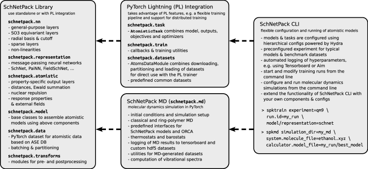
Figure 1: Overview of the five major components of the SchNetPack toolbox: the atomistic neural network library, PyTorch Lightning integration, command-line interface and molecular dynamics code. The arrows indicate dependencies between the components, i.e. components can be used independently of components on their right.

With the release of SchNetPack 2.0, major parts of the code base have been rewritten to address the changing demands on a neural network toolbox for atomistic modeling. Most importantly, SchNetPack is structured into components that can be used individually or as a unified framework. This makes it straightforward to combine some or all SchNetPack components with other PyTorch-based libraries, such as e3nn Geiger and Smidt or TorchMD Doerr et al. (2021). Fig. 1 gives an overview of the functionalities contained in each component. The core of the package is the SchNetPack library which consists of the tools required to load atomistic data and define neural network models. The library includes implementations of representations such as SchNet and PaiNN, but also provides commonly required layers to build custom atomistic representations. Furthermore, the SchNetPack library includes specific modules for the prediction of common targets, such as energies and response properties. The library can be used with pure PyTorch or a training framework of choice, as described in detail in Section II.

Alternatively, SchNetPack provides an integration of the library with the PyTorch Lightning (PL) framework Falcon et al. (2020). This enables the use of a plethora of PL features, such as customizable training loops with callbacks, distributed training supporting various accelerators and extensive support for experiment loggers such as Tensorboard Abadi et al. (2015) or Aim Arakelyan and Soghomonyan (2020). SchNetPack integrates with PL over the AtomisticTask, which is composed of models defined using the SchNetPack library, training objectives and optimizers. We further provide interfaces to popular datasets on the basis of LightningDataModule which enables automatic download and parsing of common benchmark datasets. The PL interface is described in detail in Section III.

Besides implementing neural networks with the Python API, SchNetPack 2.0 features a command-line interface (CLI) for composing models from the supplied or custom modules, which will be described in Section IV. It is powered by the Hydra Yadan (2019) framework, which allows to build hierarchical YAML configurations. The structure of this hierarchy is closely oriented on the SchNetPack PL integration, so complex models and training tasks can be described. Configured training runs can be started and modified from the command line, which makes it easy to quickly scan a large number of hyperparameters and models. User extensions to SchNetPack can be directly incorporated into the existing CLI.

Finally, SchNetPack 2.0 contains a molecular dynamics code, which makes it possible to directly apply SchNetPack models in simulations with little communication overhead. Like the rest of the code package, the MD suite is implemented in PyTorch offering full CUDA support. It retains the batch structure of the neural network toolbox, making it possible to simulate multiple systems in parallel. Building on this feature, the MD code implements an efficient way to perform ring-polymer MD simulations. A collection of thermostats and barostats is available to sample different thermodynamic ensembles. The MD code also features full CLI integration as well as a series of utilities to simplify logging and the analysis of simulation results, e.g. computation of different vibrational spectra.

Code, documentation and tutorials for SchNetPack are available on GitHub and ReadTheDocs .

II Neural network library

The SchNetPack 2.0 library provides tools and functionality to build atomistic neural networks and process datasets of molecules and materials. We have designed the library so that it can be used with vanilla PyTorch, i.e. without the need to integrate with PyTorch Lightning or the Hydra configurations. Instead we define common interfaces for datasets and models that make them ready to use with the other SchNetPack components.

A major change compared to SchNetPack 1.0 is that the data format is now fully sparse. Thus, we do no longer have to pad atomic environments with varying number of neighbors. This required a rewrite of all atomwise operations including the data pipeline as well as the message-passing and output layers. In the following, we will introduce the improved data pipeline, the pre- and postprocessing modules and the neural network models.

II.1 Data pipeline

Figure 2: The SchNetPack data pipeline. Left: ASEAtomsData provides an interface to data stored in an ASE DB and applies a sequence of preprocessing transforms. The AtomsLoader loads this data with multiprocessing and builds batches to be passed to the model. Right: example of the input dictionaries after preprocessing (top) and batching (bottom). All values of the dictionary are PyTorch tensors.

The SchNetPack data pipeline mainly consists of ASEAtomsData, adhering to the PyTorch dataset inferface, and AtomsLoader, being a PyTorch data loader with a customized collate function for batching of atomistic data. An important feature of ASEAtomsData is that one can provide a list of preprocessing transforms. They are applied in sequence to single data instances, before the latter are batched in the AtomsLoader. This is particularly useful for calculating neighbor lists, removing offsets or casting properties. The transforms will be described in detail in Section II.2. Fig. 2 gives an overview of the data pipeline and the format of the data before and after batching.

As in SchNetPack 1.0, the default PyTorch dataset ASEAtomsData is based on the database of the Atomic Simulation Environment (ASE). Larsen et al. (2017) However, the internal format has slightly changed in that it expects a dictionary of units for all properties and the atom positions. This enables automatic unit conversion without requiring internal default units. We have included the script spkconvert to add this information to older datasets. The following code snippet demonstrates how to create a new dataset:

⬇

# create new dataset

new_dataset = ASEAtomsData.create(

’./new_dataset.db’, distance_unit=’Ang’,

property_unit_dict={

’energy’:’kcal/mol’, ’forces’:’kcal/mol/Ang’

},

atomrefs = {

’energy’: [0.0, -313.5150902000774, …]

}

)

\paratoms_list = [

ase.Atoms(numbers=[1, 1, 8], positions=[…]), …

]

property_list = [{

’energy’: np.array([-450.2]),

’forces’: np.array([[0.8, -0.4, 1.3], …])}

]

new_dataset.add_systems(property_list, atoms_list)

# add metadata for custum train/test split

new_dataset.update_metadata(

train_idx=[0, 12, 53, …])

\par# create training dataset and retrieve an entry

train_data:ASEAtomsData = new_dataset.subset(

new_dataset.metadata["train_idx"]

)

some_molecule = train_data[2]

The atomistic systems are added by providing lists of ASE Atoms and dictionaries of NumPy Jones et al. (2001) arrays. Additionally, we may provide single-atom reference energies (atomrefs), which can be used for preprocessing the target properties. Both the single-atom energies and property units are stored as metadata in the ASE DB. Beyond that, additional custom metadata can be stored, such as predefined train / test splits in the code example above.

ASEAtomsData is an implementation of the abstract base class BaseAtomsData, which defines a general interface to SchNetPack datasets. This makes it possible to extend SchNetPack with custom data formats, for example for distributed datasets or special data types such as wave function files. Independent of the concrete implementation of BaseAtomsData, the format of retrieved data is a dictionary mapping from strings to PyTorch tensors, as shown in the example in Fig. 2 (right).

The AtomsLoader batches the preprocessed inputs after optional shuffling. Since systems can have a varying number of atoms, the batch dimension for atom-wise properties, such as positions and forces, runs over atoms instead of systems. The index of the corresponding system in the batch is encoded in the PyTorch tensor idx_m. Index tensors, e.g. generated by neighbor lists (idx_i, idx_j), have to be treated differently since they refer to the atom indices within a single data example. Therefore, the collate function shifts the indices to refer to the correct position within the batch.

II.2 Pre- and postprocessing transforms

Table 1: List of pre- and postprocessing transforms.

Category	Transform	Usage	Description
Neighbor lists	MatScipyNeighborList	Pre	Neighbor list implementation based on Matscipy Kermode and Pastewka (2019). This should be preferred.
	ASENeighborList	Pre	Neighbor list based on Atomic Simulation Environment.
	TorchNeighborList	Pre	Neighbor list implemented in PyTorch.
	CachedNeighorList	Pre	Wrapper for other neighbor list transforms that caches the results.
	SkinNeighborList	Pre	Wrapper around neighbor list transform that only recalculates neighbor indices after atom positions change more than a given threshold. This can be useful for structure relaxation.
	FilterNeighbors	Pre	Filter previously calculated neighbor indices.
	CountNeighbors	Pre	Count & store number of neighbors for each atom.
	WrapPositions	Pre	Wrap atom position into periodic cell.
Casting	CastMap	Pre / Post	Cast all properties according to supplied type map.
	CastTo32	Pre / Post	Cast all double precision inputs to single precision
	CastTo64	Pre / Post	Cast all single precision inputs to double precision
Scale & Offset	ScaleProperty	Pre / Post	Scale an input or result by data mean, standard deviation or given factor
	RemoveOffsets	Pre / Post	Remove single-atom reference and/or mean from an input or result
	AddOffsets	Pre / Post	Add single-atom reference and/or mean to an input or result

SchNetPack transforms are PyTorch modules that have no trainable parameters and are used for preprocessing of inputs or postprocessing of model results. Preprocessing transforms are applied before batching, i.e. they operate on single inputs. For example, virtually every SchNetPack model requires a preprocessing transform that constructs a neighbor list. However, different types of postprocessing may be demanded in the training and prediction phases. For example, a preprocessor might need to perform data augmentation during training, but not during predicting. Another example is the SkinNeighboList which takes advantage of structural similarity of sequential examples, which can be encountered in prediction tasks such as molecular dynamics simulations or structure relaxation, but not during training.

Postprocessing transforms act on batches in the result dictionary and are part of the AtomisticModel described in Section II.3. However, the loss function is supposed to be independent of postprocessing. Thus, these transforms are only enabled for prediction but not during training and evaluation. The currently supported pre- and postprocessing transforms are listed in Table 1.

In the following, we illustrate the usage of transforms at the use case of casting between single and double precision: On the one hand, double precision is required to accurately represent the comparatively small energy differences compared to the much larger scale of the total energy. On the other hand, single or even half precision is needed for fast processing of neural networks on GPUs. We solve this by applying a chain of pre- and postprocessing transforms. First, offsets such as single-atom energies are removed from the energy targets using the RemoveOffsets transform at double precision. Only then do we use the CastTo32 transform to cast all floating point inputs to single precision. Thus, the neural network is trained to predict the target without these offsets. The preprocessing modules can be set manually as follows:

⬇

atomrefs = train_data.atomrefs

train_data.transforms = [

RemoveOffsets(

remove_atomrefs=True,

atomrefs=train_data.atomrefs

),

MatScipyNeighborList(cutoff=5.),

CastTo32(),

]

Alternatively, obtaining single-atom references or other data-dependent initialization can be taken care of automatically when using PyTorch Lighting, as described in Section III.

For the final predictions, the postprocessing modules are activated, first casting the neural network prediction to double precision (CastTo64) and adding the single-atom energies afterwards (AddOffsets).

II.3 Atomistic models

Figure 3: Data processing in NeuralNetworkPotential with corresponding code.

All neural networks implemented with SchNetPack are supposed to subclass AtomisticModel. It is a PyTorch module with additional functionality that is commonly required for atomistic machine learning. In particular, it offers support for the previously described postprocessors, filtering of result dictionaries as well as a convenient mechanism to initialize and collect automatic derivatives.

While AtomisticModel can be used to implement neural networks for a broad class of tasks, SchNetPack also includes its more structured NeuralNetworkPotential. This is tailored towards ML potentials and makes use of all the features of AtomisticModel. We recommend using NeuralNetworkPotential whenever possible as it allows for an easier integration with the SchNetPack CLI. On the other hand, AtomisticModel may be employed for more general tasks. This will be demonstrated at the example of the generative model cG-SchNet in Section VI.3.

Fig. 3 depicts the processing flow of NeuralNetworkPotential. The main concept is to pass along an inputs dictionary that is modified by submodules. This enables the definition of complex neural networks with multiple inputs and outputs as just a sequence of modules. An immediate advantage is that such a model can be easily composed using configuration files and the SchNetPack CLI.

Many neural network potentials are employed for predicting response variables such as atomic forces or electric multipoles. Therefore, it is often required to calculate derivatives of model outputs w.r.t. input variables. The derivative tracking of these input variables needs to be activated before any of the modules are applied. The method AtomisticModel.collect_derivatives() can be called during initialization to scan all submodules of NeuralNetworkPotential for required derivatives. Based on this list, we enable the generation of corresponding backwards graphs using the AtomisticModel.initialize_derivatives() method during the forward pass.

In the next step, the dictionary is passed to a sequence of so-called input_modules. These may carry out preparatory steps such as calculating distances, applying strain to a lattice or adding auxiliary inputs such as external fields. The inputs then are passed on to the representation module, which constructs atom-wise features based on the input dictionary. This is often achieved by a message passing neural network that is designed to be equivariant to the symmetries of an atomistic structure (see Section II.4). The resulting features can be scalars, vectors or general multipoles and are stored under a corresponding key in the dictionary.

Finally, a sequence of output_modules computes the final results. For example, energies are often predicted as a sum over atom-wise energy contributions, which is achieved by the Atomwise module. We refer to both input and output modules as atomistic modules, since they are usually tailored to the specifics of atomistic data – in contrast to general purpose layers such as convolutions. We describe the supported operations in detail in Section II.5.

Before the results are returned, NeuralNetworkPotential makes use of two more features of AtomisticModel: First, a sequence of postprocessors is applied, if they have been enabled. This is usually only done in prediction mode, but not during training. Second, the input dictionary was updated without removing information as it passed through the model. Therefore, it still contains all the raw inputs and intermediate features. The extract_outputs method filters only the results that are supposed to be returned by the model. This is achieved in an semi-automatic fashion by scanning all submodules for potential model outputs during initialization.

II.4 Message passing and equivariant neural networks

Table 2: List of modules for message passing and equivariant neural networks.

Category	Module	Description
Radial basis	GaussianRBF Behler (2011); Schütt et al. (2017a)	Gaussian radial basis functions centered on an equidistant grid in the interval [start, cutoff]
	GaussianRBFCentered Behler (2011)	Gaussian radial basis functions centered at zero with varying widths
	BesselRBF Gasteiger, Groß, and Günnemann (2020)	$0^{\text{th}}$-order Bessel radial basis functions: $f(r)=\sin(\omega r)/r$
Cutoff	CosineCutoff Behler (2011)	$f(r)=\tfrac{1}{2}\left[1+\cos\left(\frac{\pi r}{r_{\text{cutoff}}}\right)\right],\quad r<r_{\text{cutoff}}$
	MollifierCutoff	$f(r)=\exp\left[1-\frac{1}{1-\left(\frac{r}{r_{\text{cutoff}}}\right)^{2}}\right],\quad r<r_{\text{cutoff}}$
Nonlinearity	shifted_softplus Schütt et al. (2017b)	$f(x)=\ln(0.5+0.5e^{-x})$
Sparse	scatter_add	Sum over a sparse dimension, e.g. for sums of atoms and neighbors as well as Clebsch-Gordon tensor products
SO(3) equivariance	RealSphericalHarmonics	Generates the real spherical harmonics for a batch of unit vectors
	SO3TensorProductThomas et al. (2018)	$f(x,y)_{(lm)}=\sum\limits_{l_{1}m_{1}}\sum\limits_{l_{2}m_{2}}x_{l_{1}m_{1}}y_{l_{2}m_{2}}C_{l_{1}m_{1}l_{2}m_{2}}^{lm}$
	SO3ConvolutionThomas et al. (2018)	$f(x)_{i(lm)}=\sum\limits_{j\in nbh[i]}\sum\limits_{l_{1}m_{1}}\sum\limits_{l_{2}m_{2}}x_{j(l_{1}m_{1})}W_{l_{2}}(r_{ij})Y_{l_{2},m_{2}}(\vec{r}_{ij}/r_{ij})C_{l_{1}m_{1}l_{2}m_{2}}^{lm}$
	SO3GatedNonlinearity	$f(x)_{i(lm)}=x_{i(l,m)}\sigma(x_{i(0,0)})$
	SO3ParametricGatedNonlinearityWeiler et al. (2018)	$f(x)_{i(lm)}=x_{i(l,m)}\sigma(g_{\theta}(x_{i(0,0)}))$

SchNetPack provides the tools to build a wide variety of atomistic machine learning models, even beyond neural networks. However, our focus remains on end-to-end neural networks that build atom-wise representations. In recent years, the two concepts that have dominated this field are neural message passing Schütt et al. (2017a); Gilmer et al. (2017) and equivariant neural networks Thomas et al. (2018); Weiler et al. (2018). SchNetPack comes with four implemented atomistic representations:

• SchNetSchütt et al. (2017b, 2018a): The name-giving continuous-filter convolutional network motivated the creation of SchNetPack. It uses rotationally-invariant filters and, although it is no longer the most accurate model five years after it was first proposed, it is pretty lightweight.

• FieldSchNetGastegger, Schütt, and Müller (2021): An extension of SchNet that makes use of atomic dipole features to handle external fields in order to model response properties and solvent effects.

• PaiNNSchütt, Unke, and Gastegger (2021): The successor to SchNet that uses equivariant message passing in Cartesian space.

• SO3net: A minimalist SO(3)-equivariant neural network in the spirit of Tensor Field Networks Thomas et al. (2018) or NequIP Batzner et al. (2022) that showcases the spherical harmonics and Clebsch-Gordan tensor product modules of SchNetPack.

Table 2 gives an overview of related modules that we provide for building atomistic representations. This includes radial basis and cutoff functions, nonlinearities and SO(3) equivariant layers. Naturally, these are only additions to the large variety of modules already included in PyTorch, e.g. the SiLU nonlinearity Hendrycks and Gimpel (2016), which has been employed in many recent atomistic neural networks Gasteiger, Groß, and Günnemann (2020); Schütt, Unke, and Gastegger (2021); Batzner et al. (2022).

By convention, the atomistic representations in SchNetPack have the shape $(n_{\text{atoms}},[n_{\text{spatial}},]n_{\text{features}})$, where the first dimension runs over all atoms in the batch, the second is reserved for optional directional channels of equivariant representations and the last is reserved for feature channels. In this format, it is straightforward to define message passing operations using the atom and neighbor indices obtained from neighbor list transforms during preprocessing. For example, the continuous-filter convolution of SchNet Schütt et al. (2017b) can be implemented as follows:

⬇

# inputs:

# x: atom-wise representation

# Wij: radial filters

# idx_i, idx_j: neighbor list indices

x_j = x[idx_j]

x_ij = x_j * Wij

y = scatter_add(x_ij, idx_i, dim_size=x.shape[0])

The second (optional) dimension of atom-wise representations is reserved for the directional features of equivariant neural networks. For the vectorial features, e.g. in case of PaiNN, this corresponds to the Cartesian $(x,y,z)$-directions ($n_{\text{spatial}}=3$). In case of SO(3)-equivariant features, the dimensions correspond to the real spherical harmonics $Y_{l,m}$ as follows: $[Y_{0,0},Y_{1,-1},Y_{1,0},Y_{1,1},Y_{2,-2},Y_{2,-1},\dots]$.

For the implementation of tensor product modules required for SO(3)-equivariant models, the Clebsch-Gordan coefficients $C_{l_{1}m_{1}l_{2}m_{2}}^{lm}$ are precomputed during initialization and stored in sparse format with the non-zero coefficients clebsch_gordan and three combined index tensors idx_in_1, idx_in_2 and idx_out corresponding to the tuples $(l_{1},m_{1})$, $(l_{2},m_{2})$ and $(l,m)$, respectively. This enables fast calculation of tensor products. For example, the SO3TensorProduct module calculating

$$f(x,y)_{(lm)}=\sum\limits_{l_{1}m_{1}}\sum\limits_{l_{2}m_{2}}x_{l_{1}m_{1}}y_{l_{2}m_{2}}C_{l_{1}m_{1}l_{2}m_{2}}^{lm},$$

can be implemented as follows:

⬇

# x, y: atom-wise features $[n_\text{atoms}, (l_\text{max}+1)^2, n_\text{features}]$

h = x[:, idx_in_1, :] \ * y[:, idx_in_2, :] \ * clebsch_gordan[None, :, None]

z = scatter_add(h, idx_out,

dim_size=(lmax + 1) ** 2, dim=1)

The combined indices idx_in_1 and idx_in_2 select the spherical basis functions to be multiplied by the non-zero Clebsch-Gordan coefficients. The third index tensor is used for summation of terms mapping to the same $(l,m)$ using scatter_add analogous to the atom accumulation in the message passing shown above. Similarly, SO3Convolutions or other custom SO(3)-equivariant modules can be implemented in a straightforward fashion.

II.5 Atomistic modules

Table 3: List of atomistic modules for preparing the raw inputs and predicting various properties.

Category	Module	Description
Distances	PairwiseDistances	Compute pair-wise distances from indices provided by a neighbor list transform.
	FilterShortRange	Separate distances below a short-range cutoff from all supplied distances.
Properties	Atomwise Behler and Parrinello (2007)	Predicts a property from atom-wise contributions and accumulates global prediction using sum or average, e.g. for the energy $E=\sum\limits_{i=1}^{n_{\text{atoms}}}E(x_{i})$
	DipoleMomentGastegger, Behler, and Marquetand (2017); Veit et al. (2020); Schütt, Unke, and Gastegger (2021)	Predicts dipole moments from latent partial charges and (optionally) local, atomic dipoles: $$\vec{\mu}=\sum\limits_{i=1}^{n_{\text{atoms}}}q(x_{i})\vec{r}_{i}\left[+\vec{\mu}_{\text{atomic}}(\vec{x}_{i})\right]$$
	Polarizability Schütt, Unke, and Gastegger (2021)	Predicts polarizability using the tensor rank factorization: $$\alpha=\sum_{i=1}^{N}\alpha_{\text{0}}(x_{i})\,I_{3}+\vec{\nu}(\vec{x}_{i})\otimes\vec{r_{i}}+\vec{r_{i}}\otimes\vec{\nu}(\vec{x}_{i})$$
	Aggregation	Aggregate predictions from multiple atomistic modules to a single output variable, e.g. calculating the energy prediction as the sum of short-range and long-range energies.
Potentials	EnergyCoulomb	Compute Coulomb energy from a set of (latent) point charges.
	EnergyEwald	Compute the Coulomb energy of a set of (latent) point charges inside a periodic box using Ewald summation.
	ZBLRepulsionEnergy Ziegler and Biersack (1985); Unke et al. (2021c)	Computes a Ziegler-Biersack-Littmark-style repulsion energy.
Response	StaticExternalFields	Input module for setting up dummy external fields. These do not receive inputs, but are only used to calculate response properties with autograd.
	Strain	Input module for setting up dummy strain. It does not receive inputs, but is only used to calculate the stress tensor using autograd.
	Forces	Output module that predicts forces and stress as response of the energy prediction w.r.t. the atom positions and strain.
	Response Gastegger, Schütt, and Müller (2021)	Output module that computes different response properties by taking derivatives of an energy model. Supports forces, stress, Hessian, dipole moment (and its derivatives) polarizability (and its derivatives), shielding tensor as well as nuclear spin-spin coupling.

Atomistic modules are specific to the properties to be predicted and informed by the regularities of the underlying physics. In contrast to general purpose layers, such as non-linearities or convolutions, they are supposed to directly operate on the input dictionary which is passed through the model, as described in Section II.3. This makes it easy to compose complex atomistic neural networks. Thus, the input and output modules of a NeuralNetworkPotential are usually atomistic layers.

Table 3 describes the atomistic modules currently supported by SchNetPack. A range of output modules is concerned with predicting atomistic properties from the previously generated representations. The most common is Atomwise, which predicts a property as a sum of atom-wise contributions, e.g. when predicting potential energy surfaces. Behler and Parrinello (2007); Bartók et al. (2010); Schütt et al. (2017a) We have also included specialized layers for tensorial properties such as dipole moments and polarizability tensors. Beyond that, it is often helpful for generalization to include physically-inspired terms in the energy prediction. This is includes electrostatic modules and ZBL potentials Ziegler and Biersack (1985) for nuclear-nuclear repulsion.

Virtually every neural network potential requires the PairwiseDistances module as an input layer, which makes use of the indices calculated by a neighbor list during preprocessing. The distance calculation being part of the model enables straightforward automatic differentiation w.r.t. to atom positions. The Forces module provides atomic forces and the stress tensor as derivatives w.r.t. atomic positions and strain. Beyond that, SchNetPack includes the Response module, which additionally supports response properties w.r.t. external (electric or magnetic) fields as well as higher-order derivatives, e.g. for polarizability or shielding tensors. The FieldSchNet example in Section VI.2 demonstrates how this can be employed in practice.

III PyTorch Lightning integration

While it is possible to use the previously described SchNetPack library on its own, a third-party framework that takes care of the boilerplate code required for training and validation can significantly speed up the development process. We chose PyTorch Lightning Falcon et al. (2020) as the default training framework for SchNetPack, as it supports a wide variety of hardware devices and distribution strategies. In the following, we describe how LightningModule and LightningDataModule are employed to predefine common datasets, tasks and workflows.

The PyTorch Lightning trainer expects a LightningModule which defines the learning task, i.e. a combination of model definition, objectives and optimizers. SchNetPack provides the AtomisticTask, that integrates the AtomisticModel, as described in Section II.3, with PyTorch Lightning. The task configures the optimizer, defines the training, validation and test steps, calculates the loss and logs training metrics. For this purpose, AtomisticTask expects a list of of ModelOutputs, which map a target property to a key in the results dictionary of the AtomisticModel. Additionally, ModelOutput requires a loss function and (optionally) a list of Metrics that are tracked during training and validation. Given a model my_neural_network_potential that stores the predictions energy and forces in the result dictionary, the task of training a neural network potential can be defined as follows:

⬇

output_energy = ModelOutput(

name="energy",

loss_fn=torch.nn.MSELoss(),

loss_weight=0.01,

metrics={"MAE": torchmetrics.MeanAbsoluteError()}

)

\paroutput_forces = ModelOutput(

name="forces",

loss_fn=torch.nn.MSELoss(),

loss_weight=0.99,

metrics={"MAE": torchmetrics.MeanAbsoluteError()}

)

task = AtomisticTask(

model=my_neural_network_potential,

outputs=[output_energy, output_forces],

optimizer_cls=torch.optim.AdamW,

optimizer_args={"lr": 1e-4}

)

To define a dataset, we subclass PyTorch Lightning data modules with AtomsDataModule. This combines the data classes introduced in Section II.1 with code for preparation, setup and partitioning into train, validation and test splits. The default splitting strategy is random sampling, however other strategies, such as sub-sampling predefined partitions or keeping certain groups of structures in the same partition, are supported as well. One may provide separate preprocessing transforms for train, validation and test splits if needed, e.g. when data augmentation is only required for the training data.

Beyond that, data modules may take care of setting up the data for distributed training, e.g. copying the data to a local storage. We provide specialized AtomsDataModules for common benchmark sets, that automatically download and parse the data. Currently supported datasets include QM9 Ramakrishnan et al. (2014), (r)MD17 Chmiela et al. (2017); Christensen and Von Lilienfeld (2020), MD22 Chmiela et al. (2022), OMDB Olsthoorn et al. (2019), and the MaterialsProject Jain et al. (2013). Additional datasets can be added by sub-classing AtomsDataModule and overriding the prepare_data method with custom code for downloading and parsing.

Here is an example of how the MD17 datamodule can be used:

⬇

ethanol_data = MD17(

"/path/to/data.db",

molecule=’ethanol’,

batch_size=10,

num_train=1000,

num_val=1000,

transforms=[

MatScipyNeighborList(cutoff=5.),

RemoveOffsets(MD17.energy, remove_mean=True),

CastTo32()

],

num_workers=1

)

ethanol_data.prepare_data()

ethanol_data.setup()

\par# iterate over training batches

for batch in ethanol_data.train_dataloader():

print(batch)

The passed transforms are applied to all partitions in this case and RemoveOffsets is automatically initialized with the training data statistics. Manual calling of prepare_data, which downloads and parses the data, and setup, which creates and loads the partitions, is necessary here because we retrieve the data loader and iterate over the training data. Instead, one may pass the data module directly to the PyTorch Lightning trainer class, which ensures that prepare_data is called exactly once. However, the setup method is called in every process of distributed training.

Finally, we put everything together by passing the task and data module to the PyTorch Lightning trainer, which executes the training loop:

⬇

trainer = pl.Trainer()

trainer.fit(task, datamodule=ethanol_data)

The training process can be adapted by callbacks and loggers as well as specifying options to train on several (distributed) devices. Please refer to the PyTorch Lightning documentation  for more information.

IV Configuration and command-line interface

⬇

defaults:

- override /model: nnp

- override /data: qm9

\parrun:

experiment: qm9_${globals.property}

\parglobals:

cutoff: 5.

lr: 5e-4

property: energy_U0

aggregation: sum

\pardata:

transforms:

- _target_: schnetpack.transform.SubtractCenterOfMass

- _target_: schnetpack.transform.RemoveOffsets

property: ${globals.property}

remove_atomrefs: True

remove_mean: True

- _target_: schnetpack.transform.MatScipyNeighborList

cutoff: ${globals.cutoff}

- _target_: schnetpack.transform.CastTo32

\parmodel:

output_modules:

- _target_: schnetpack.atomistic.Atomwise

output_key: ${globals.property}

n_in: ${model.representation.n_atom_basis}

aggregation_mode: ${globals.aggregation}

postprocessors:

- _target_: schnetpack.transform.CastTo64

- _target_: schnetpack.transform.AddOffsets

property: ${globals.property}

add_mean: True

add_atomrefs: True

\partask:

outputs:

- _target_: schnetpack.task.ModelOutput

name: ${globals.property}

loss_fn:

_target_: torch.nn.MSELoss

metrics:

mae:

_target_: torchmetrics.regression.MeanAbsoluteError

rmse:

_target_: torchmetrics.regression.MeanSquaredError

squared: False

loss_weight: 1.

Figure 4: SchNetPack experiment config for prediction tasks of QM9 properties with the Atomwise output layer.

SchNetPack training runs can be defined using the hierarchical configurations framework Hydra Yadan (2019). This enables configuration of complex neural network potentials using YAML files, provides powerful command-line tools and makes it easy for developers to extend SchNetPack with external code.

The main command of the SchNetPack CLI is spktrain, which creates a new run directory and starts the training of a configured model. We refer to a predefined configuration including model, task, data, etc. as an experiment, which can be started as follows:

⬇

spktrain experiment=qm9_atomwise

This starts the training with the default settings for energies of the QM9 dataset. The script first prints the flattened config of the run, i.e. the config when specified in a single YAML file. Fig. 4 instead shows the hierarchical experiment configuration that this has been derived from.

IV.1 Structure of the configuration

The structure of configurations is heavily oriented on the building blocks introduced in Sections II and III. Due to its hierarchy, we only have to override the defaults and make use of reusable, predefined config groups, e.g. for the model or the dataset. The major config groups of SchNetPack are:

• run: Definition of run-specific variables, such as the run id as well as directories, where the metrics are logged and the trained model and the data will be stored. If no run id is given, SchNetPack will create a unique hash.

• globals: Custom variables to be used across the whole config can be added here. This is possible through the use of the interpolation syntax ${globals.variable}.

• data: Definition of the dataset as described by AtomsDataModule (see Section III).

• model: Definition of the AtomisticModel (see Section II.3).

• task: Configuration of the AtomisticTask, including model outputs, losses and optimizers.

• trainer: Arguments to be passed to the PyTorch Lightning Trainer.

• callbacks: A list of callbacks to be passed to the Trainer

• logger: Configuration of training metric loggers, such as Tensorboard Abadi et al. (2015) or Aim Arakelyan and Soghomonyan (2020).

• seed: Sets the random seed for PyTorch and Pytorch Lightning.

The first lines of the configuration in Fig. 4 show how the model and data are overridden with the default config templates (nnp and qm9) for the neural network potential and the QM9 dataset, respectively. The data and model templates are further modified in lines 14-36 by specifying pre- and postprocessing transforms, output modules as well as model outputs with losses and metrics to be tracked. The special key _target_ enables automatic instantiating of objects. For example, in the list of model outputs in Fig. 4 (lines 26-30), the Atomwise module is initialized with the given parameters. Here, the target object is not restricted to be a SchNetPack module, but can also be a class provided by a third-party Python package. This makes it straightforward to extend SchNetPack with custom layers, losses and models.

IV.2 Modifying configurations from command line

We have shown above how a training run specified by the experiment config can be started from the command line. Beyond that, the configuration of a run can also be directly modified using the CLI. For example, training neural network potentials with a different representation and using a larger learning rate than the default can be achieved as follows:

⬇

spktrain experiment=qm9_atomwise \ model/representation=schnet globals.lr=1e-3

Note that when setting config groups to a preconfigured template, a slash ’/’ is used, while when setting a value in the YAML, the dot "." is used to navigate the hierarchy. Finally, custom experiment configs can be added by setting a user config directory:

⬇

spktrain -config-dir=/configdir \ experiment=my_experiment

The config directory needs to follow the structure of the config, e.g. the experiment should be located at /configdir/experiment/my_experiment.yaml.

IV.3 Extending SchNetPack

The modular design of SchNetPack configurations allows for seamless extension of the framework with additional models and learning tasks, including their integration into the CLI. For example, the data pipeline and training flow of the framework could be kept while changing the representation block of a neural network potential. This enables a quick and standardized comparison of different approaches. To this end, one may implement a small python package containing the network building blocks as well as a custom configuration file for instantiating the new representation. The training can be started with spktrain using the familiar CLI. By providing Hydra with the location of the additional configuration files in the extension package, the representation can simply be switched to the new network as if it was part of SchNetPack. This means that developers are able to build atomistic ML models on top of SchNetPack by exchanging only selected building blocks and avoiding as much boilerplate code as possible. The example in Section VI.3 shows that this is not only possible with neural network potentials but also with more complex atomistic learning tasks such as a generative model for molecules.

V Molecular dynamics simulations

In addition to the neural network library, SchNetPack 2.0 contains the schnetpack.md code for carrying out molecular dynamics simulations. This MD environment is structured in a modular way in order to facilitate development and interfacing with different ML potentials. Since all routines are implemented in PyTorch, models based on AtomisticModel can be used with minimal communication overhead and full GPU capabilities.

The MD code performs several core tasks during each simulation step. It keeps track of the positions $\mathbf{R}$ and momenta $\mathbf{p}$ of all nuclei, computes the forces $\mathbf{F}$ acting on them and uses the latter to integrate the equations of motion. In SchNetPack, these tasks are distributed between different modules, which are sketched in Fig. 5a. The md.System class contains all information on the current system state (e.g. nuclear positions and momenta). The md.Integrator propagates the positions and momenta of the system. In order to carry out this update, the nuclear forces are required. These are computed by an md.Calculator, which takes the positions of atoms and returns the forces due to the potential. Typically, the Calculator connects to a previously trained machine learning model. All these modules are linked together in the md.Simulator class, which contains the main MD loop and calls the three previous modules. The simulator can further be modified with so-called simulation hooks to control aspects like sampling (e.g. thermostats or barostats) or logging (Fig. 5b). In the following, we will describe the MD modules in detail.

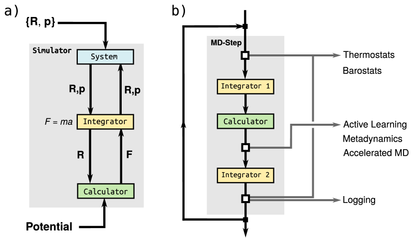
Figure 5: a) Basic MD workflow. b) internal structure of a single simulation step, indicating points at which different hooks can be applied to modify a simulation.

V.1 System

The md.System class keeps track of the state of the simulated system and collects all associated quantities (e.g. positions, momenta, atom types, simulation cells, …). This information is stored in multi-dimensional PyTorch tensors, which makes it possible to vectorize many operations and e.g. simulate several different molecules as well as different replicas of a molecule in a single step. The shape convention of the system tensors is similar to the one used in the atomistic representations, with an added replica dimension $(n_{\text{replicas}},n_{\text{atoms}},\ldots)$. This replica dimension collects different replicas of the same molecules and can be used, for example, in ring-polymer MD simulations. In addition, the md.System class provides utilities for computing different quantities relevant for MD simulations, such as temperature and pressure.

Structural information can be added to a md.System instance via the load_molecules function using ASE Atoms objects. The function operates on either a single object or a list of Atoms and automatically takes care of simulation cells and periodic boundary conditions. If a list is provided, multiple molecules can be loaded at once. During loading, it is necessary to specify the number of replicas and the units of length used for the input structures. The latter is required, since the MD code uses its own internal unit system and automatically converts the inputs. The creation of a md.System instance is demonstrated in the following example:

⬇

# Read structures with ASE

molecule = ase.io.read("molecule.xyz")

\par# Create system instance and load molecule

md_system = schnetpack.md.System()

md_system.load_molecules(

molecule,

n_replicas=1,

position_unit_input="Angstrom"

)

By default, momenta are set to zero upon creating a System. If desired, a md.Initializer can be used to draw the momenta from different distributions corresponding to a certain temperature. The following example uses the UniformInit initializer, which draws momenta from a random uniform distribution and rescales them to a certain temperature. Other routines, e.g. drawing from a Maxwell—Boltzmann distribution, are also available.

⬇

md_initializer = md.UniformInit(

300, # system temperature in K

remove_center_of_mass=True,

remove_translation=True,

remove_rotation=True,

)

\par# Initialize the system momenta

md_initializer.initialize_system(md_system)

A md.Initializer may also be used to center the molecular structure on the center of mass and remove all translational and rotational components of the momenta, as demonstrated in the code snippet above.

V.2 Integrator

As the name suggests, the md.Integrator is used to integrate the equations of motion based on the nuclear forces. Two integration schemes are implemented in SchNetPack 2.0: The first md.VelocityVerlet implements the Velocity Verlet algorithm which evolves the system in a purely classical manner. The second integrator md.RingPolymer performs ring-polymer MD simulations, which recover a certain degree of nuclear quantum effects. Both integrators use a three step scheme and come with special NPT variants for constant pressure simulations.

To initialize an md.Integrator, one has to specify the integration time step in units of femtoseconds. In the following example, we use the Velocity Verlet algorithm with a time step of $\Delta t=0.5$ fs:

⬇

time_step = 0.5 # fs

\par# Set up the integrator

md_integrator = md.VelocityVerlet(time_step)

V.3 Calculator

The nuclear forces required for the integrator are provided by a md.Calculator. It serves as an interface between a computation method (e.g. the neural network potential) and the MD code. The calculator takes the current positions of the md.System and other structural properties (simulation cells, etc) and converts them to a format suitable for the computation method. Once all requested properties (e.g. forces) have been computed, the md.Calculator collects the results and reshapes the tensors back into the md.System format. Different custom calculators can be derived from the MDCalculator base class. SchNetPack comes with several predefined calculators, such as the SchNetPackCalculator which can be directly used with trained SchNetPack models, the OrcaCalculator for the ORCA quantum chemistry packageNeese (2012), as well as ensemble variants of these calculators for adaptive sampling. In the following, we describe the basic usage of the SchNetPackCalculator.

Since the core of the calculator is a SchNetPack AtomisticModel, interatomic distances need to be computed during the MD. This is done with the NeighborListMD wrapper, which can be used with any neighbor list transform (Tab. 1). It takes the basic neighbor list module, a cutoff radius and a buffer region as input (both use the same length units as the model). The introduction of a buffer region improves performance, since a MD neighbor list only needs to be recomputed once the structural changes exceeding the buffer region. In the following, we use the MatScipyNeighborlist, with a 5 Å cutoff and 2 Å buffer region:

⬇

from schnetpack.md.neighborlist_md \ import NeighborListMD

from schnetpack.transform \ import MatScipyNeighborList

\parmd_neighborlist = NeighborListMD(

cutoff=5.0, # cutoff

cutoff_shell=2.0, # buffer region

MatScipyNeighborList,

)

To initialize md.SchNetPackCalculator, we need to provide it with the path to a trained model and the key of the forces in the output dictionary. Moreover, the units that the calculator expects for positions and energy in order to properly convert between MD and calculator unit systems need to be specified. Force units are inferred automatically based on these two inputs. Optionally, one may provide an energy_key to store the potential energies in the md.System class. Additional properties (e.g. dipole moments for infrared spectra, etc.) can be requested with the required_properties argument. A typical SchNetPack NeuralNetworkPotential trained on the MD17 data would be initialized as follows:

⬇

from schnetpack.md.calculators \ import SchNetPackCalculator

\parmd_calculator = SchNetPackCalculator(

"<PATH/TO/MODEL>", # path to stored model

"forces", # force key

"kcal/mol", # energy units

"Angstrom", # length units

md_neighborlist, # neighbor list defined above

energy_key="energy", # potential energies

required_properties=[], # additional properties

)

V.4 Simulator

The md.Simulator loops over a series of time steps, calls the individual MD modules in the appropriate order and updates the system state. Its internal structure is depicted in Fig 5b. Assuming a md.System, md.Integrator and md.Calculator have been created as described above, the setup is straightforward:

⬇

md_simulator = schnetpack.md.Simulator(

md_system,

md_integrator,

md_calculator,

simulation_hooks=[],

)

Simulation hooks can be used to modify a simulation analogous to transforms in the neural network library and are described in Sec. V.5. The required floating point precision and the computational device to be used can be set by the usual PyTorch directives:

⬇

md_device = "cpu"

md_precision = torch.float32

\parmd_simulator = md_simulator.to(md_precision)

md_simulator = md_simulator.to(md_device)

The simulate routine runs the simulation with the number of simulation steps as an argument:

⬇

# simulate for 100 steps

md_simulator.simulate(100)

Since the md.Simulator keeps track of the simulation and system state, repeated calls of calculate will resume the simulation.

V.5 Simulation hooks

Simulation hooks can be used to tailor a simulation to specific needs, improving the customizability of the SchNetPack 2.0 MD code. A SimulationHook can be thought of as a set of instructions for the Simulator, which are performed at certain points of a MD step. Depending on which time they are called and which actions they encode, simulation hooks can achieve a wide range of tasks.

Fig 5b shows an overview at which points simulation hooks can be applied during a Simulator step. If a SimulationHook is applied before and after the integration half-step updating the momenta, it could control temperature and pressure of the system in the form of thermostats and barostats. Acting directly after the md.Calculator, a hook may implement custom sampling schemes such as metadynamics or adaptive sampling.Laio and Parrinello (2002); Gastegger, Behler, and Marquetand (2017) When called after the second integration step, simulation hooks can be used to collect and store information on the system for analysis. A list of multiple hooks can be passed to a simulator, which enables control of a simulation in various manners. An overview of all simulation hooks currently implemented in SchNetPack 2.0 is shown in Tab. 4. In the following, we will give a brief overview on how to apply thermostat hooks and collect simulation data:

Table 4: Overview of simulation hooks (and data streams).

Category	Hook	Description
Basic	SimulationHook	Abstract base class for deriving hooks.
	RemoveCOMMotion	Periodically remove center of mass translation and rotation.
Thermostats	BerendsenThermostat	Simple velocity rescaling thermostat.Berendsen et al. (1984)
	LangevinThermostat	Basic stochastic Langevin thermostat.Bussi and Parrinello (2007)
	NHCThermostat	Nosé–Hoover chain thermostat.Martyna, Klein, and Tuckerman (1992)
	GLEThermostat	Stochastic generalized Langevin equantion (GLE) colored nose thermostat.Ceriotti, Bussi, and Parrinello (2010)
	PILELocalThermostat	Path integral Langevin equation (PILE) thermostat for ring-polymer MD.Ceriotti et al. (2010)
	PILEGlobalThermostat	Global variant of PILE, applies stochastic velocity rescaling to the ring-polymer centroid.Ceriotti et al. (2010)
	TRPMDThermostat	Thermostated ring-polymer variant of the PILE thermostat.Rossi, Ceriotti, and Manolopoulos (2014)
	RPMDGLEThermostat	GLE colored noise thermostat for ring-polymer MD.Ceriotti, Bussi, and Parrinello (2010)
	PIGLETThermostat	Version of GLE where every normal mode is thermostated seperately.Uhl, Marx, and Ceriotti (2016)
	NHCRingPolymerThermostat	Nosé–Hoover chain thermostat for ring-polymer MD.Ceriotti et al. (2010)
Barostats	NHCBarostatIsotropic	Combined Nosé–Hoover chain thermostat and barostat for isotropic cell fluctuations.Martyna et al. (1996)
	NHCBarostatAnisotropic	Combined Nosé–Hoover chain thermostat and barostat for anisotropic cell fluctuations.Martyna et al. (1996)
	PILEbarostat	Stochastic PILE barostat for ring-polymer MD.Kapil et al. (2019)
Logging	CheckPoint	Periodically store the system state for restarting.
	TensorBoardLogger	Log system information (e.g. temperature, energy) in TensorBoard format.
	FileLogger	Log system information to a custom HDF5 dataset. Data streams are used to store different data groups.
	MoleculeStream	Data stream for storing structural information with the FileLogger.
	PropertyStream	Data stream for storing system properties with the FileLogger.

Temperature and pressure control

Constant temperature (NVT) and constant pressure (NPT) simulations can be performed using thermostat and barostat hooks. A simple example is the stochastic Langevin thermostat implemented in LangevinThermostat. It requires a time constant (in fs) and bath temperature (in K) to initialize:

⬇

from schnetpack.md.simulation_hooks \ import LangevinThermostat

\parthermostat_hook = LangevinThermostat(

300.0, # bath temperature in K

100.0, # time constant in fs

)

Callbacks and Logging

The FileLogger hook is the primary way to collect and store MD simulation data. The kind of information stored is controlled via two types of data streams: The MoleculeStream stores structural information and velocities during the simulation, while PropertyStream collects properties computed by the md.Calculator. To reduce file I/O overhead, the FileLogger collects a certain number of steps into a buffer before it is written to an HDF5 file at once.

The FileLogger requires the destination path, the buffer size and the data streams. In addition, the logging frequency can be specified:

⬇

from schnetpack.md.simulation_hooks \ import callback_hooks

\par# Set up data streams

data_streams = [

# store positions and velocities

callback_hooks.MoleculeStream(

store_velocities=True

),

# store energies

callback_hooks.PropertyStream(

target_properties=["energy"]

),

]

\par# Create the file logger

file_logger_hook = callback_hooks.FileLogger(

"simulation.hdf5", # path to the log file

100, # size of the buffer

data_streams=data_streams,

every_n_steps=1, # logging frequency

)

V.6 Using the HDF5 dataset

SchNetPack 2.0 simulation data, stored in a HDF5 dataset as described previously, can be accessed with the HDF5Loader class to retrieve structures or perform analysis. Properties collected during simulation can be extracted with the get_property function. It takes the name of a property and an indicator, whether the property relates to the whole system or particular atoms:

⬇

from schnetpack.md.data \ import HDF5Loader

\parmd_data = HDF5Loader("simulation.hdf5")

\parenergy = md_data.get_property(

"energy", atomistic=False

)

The HDF5Loader comes with multiple predefined functions to extract specific properties, such as temperature or pressure. All of those receive a molecule index mol_idx and replica index repica_idx as additional inputs. The former is used to extract information of a particular system when multiple are simulated at the same time, while the latter is used to target specific replicas, e.g. in ring-polymer MD. The default behavior is to target the first system and compute the average (centroid) over all replicas. Finally, convert_to_atoms allows structures to be extracted as a list of ASE Atoms objects.

SchNetPack 2.0 provides the module md.data.spectra to compute different vibrational spectra directly from an HDF5Loader instance. Routines for power spectra (PowerSpectrum, requires momenta), infrared (IR) spectra (IRSpectrum, requires dipole moments) and Raman spectra (RamanSpectrum, requires polarizabilities) are available. For example, the power spectrum can be computed as follows:

⬇

from schnetpack.md.data \ import PowerSpectrum

\par# Initialize the spectrum

spectrum = PowerSpectrum(md_data, resolution=2048)

\par# Compute the spectrum

spectrum.compute_spectrum()

\par# Get frequencies and intensities

frequencies, intensities = spectrum.get_spectrum()

V.7 Molecular Dynamics Configuration and Command Line Interface

Similar to the neural network package, MD simulations can be configured using the Hydra framework. The central command of the SchNetPack MD CLI is spkmd, which sets up everything for a basic MD simulation and creates a simulation directory. Runs can be configured via predefined config groups and command-line overrides. Moreover, since the Hydra CLI is able to instantiate classes from YAML configs, it is straightforward to integrate external modules, such as custom calculators for simulations.

A standard spkmd run requires the following inputs:

⬇

spkmd simulation_dir=<DIR> system.molecule_file=<XYZ> calculator.model_file=<MODEL> calculator.neighbor_list.cutoff=<CUTOFF>

where simulation_dir indicates the simulation directory, system.molecule_file the file containing the structures to be simulated and calculator.model_file and calculator.neighbor_list.cutoff specify the path to the previously trained neural network potential and the cutoff radius used in the model. This starts a MD run with a predefined default configuration, which corresponds to a NVE simulation where features such as logging and checkpointing have already been set up.

Like in the neural network package, an MD config is structured into different config groups:

• uncategorized, general settings, such as device, precision, random seed and simulation directory.

• calculator: Definition of the MD calculator (see Sec. V.3).

• system: Definition of the MD system, including loading of structures and initial conditions (see Sec. V.1).

• dynamics: Definition of the overall MD loop (Sec. V.4). Contains the subgroups:

  • integrator: Integrator settings (Sec. V.2)

  • thermostat: Temperature control.

  • barostat: Pressure control.

  • simulation_hook: General hooks for sampling (Sec. V.5).

• callbacks: Definition of hooks for callback and logging.

These groups can be used to further configure the simulation, e.g. by adding a thermostat or changing integrator settings (see e.g. Sec VI.2).

MD simulations can be started using full or partial config files in YAML format as input. For example, it is possible to create a basic config file by calling spkmd with the --cfg job flag and edit it for a particular application. An existing config file can then be loaded with the load_config option:

⬇

spkmd simulation_dir=<DIR> load_config=<CONFIG-FILE>

It is still possible to further modify the simulation via other command line overwrites.

VI Example applications

This section features some basic and advanced applications of SchNetPack. First, we demonstrate how to train atomistic neural networks on the supported benchmark datasets. In a second example, we showcase the prediction of response properties at the example of a custom dataset. Finally, we demonstrate how SchNetPack can be extended with custom code to train a generative neural network for the inverse design of 3d structures.

VI.1 Potential energy surfaces and property prediction

Table 5: Mean absolute and mean squared error for various neural networks trained with SchNetPack on prediction task on the QM9 and rMD17 benchmark datasets. The errors are averaged over three repetitions.

Dataset	Property	Unit	Metric	SchNet	PaiNN	SO3net (l${}_{\text{max}}$=1)	SO3net (l${}_{\text{max}}$=2)
QM9	U0	meV	MAE	9.6	5.7	6.8	6.4
			RMSE	21.9	15.3	16.2	17.1
QM9	$\mu$	Debye	MAE	0.022	0.011	0.018	0.014
			RMSE	0.044	0.026	0.038	0.033
rMD17 / Aspirin	$E$	meV	MAE	13.5	3.8	3.8	2.6
			RMSE	18.3	5.9	5.7	3.8
	$F$	meV/Å	MAE	33.2	12.8	12.7	9.0
			RMSE	49.5	21.7	19.6	14.5
rMD17 / Paracetamol	$E$	meV	MAE	8.4	2.1	2.2	1.4
			RMSE	11.2	2.9	3.0	1.9
	$F$	meV/Å	MAE	26.1	9.0	8.9	6.0
			RMSE	40.0	14.7	13.8	10.0

Table 6: Training and validation time per epoch for models trained on QM9 and rMD17 tasks using an Nvidia A100.

Task	Model	# params	time / epoch
QM9, U0 110k / 10k bs 100	SchNet	432k	1 min 14 sec
	PaiNN	589k	1 min 13 sec
	SO3net (l${}_{\text{max}}$=1)	283k	1 min 16 sec
	SO3net (l${}_{\text{max}}$=2)	341k	2 min 29 sec
rMD17, E+F, Aspirin 950 / 50 bs 10	SchNet	432k	7 sec
	PaiNN	589k	6 sec
	SO3net (l${}_{\text{max}}$=1)	283k	7 sec
	SO3net (l${}_{\text{max}}$=2)	341k	10 sec

The datasets QM9 Ramakrishnan et al. (2014) and MD17 Chmiela et al. (2017) have become established benchmarks in the development of atomistic representations. Here, we use the revised MD17 (rMD17) dataset for which the energies and forces have been recomputed with higher accuracy Christensen and Von Lilienfeld (2020). We have trained models using three representations SchNet, PaiNN and SO3net. For the latter, we have explored setting the maximum angular moment to $l_{\text{max}}\in\{1,2\}$.

We have predicted the inner energy $U_{0}$ and the total dipole moment $\mu$ from the properties in QM9 with two separate models. The configuration qm9_atomwise for $U_{0}$ is given in Fig. 4. The only difference of the qm9_dipole configuration is the use of the DipoleMoment output module:

⬇

model:

output_modules:

- _target_: schnetpack.atomistic.DipoleMoment

dipole_key: ${globals.property}

n_in: ${model.representation.n_atom_basis}

predict_magnitude: True

use_vector_representation: False

postprocessors:

- _target_: schnetpack.transform.CastTo64

If the representation supports equivariant vector features, which is the case for PaiNN and SO3net, we use atomic dipoles in the output layer Schütt, Unke, and Gastegger (2021) by setting use_vector_representation=True (see Table 3).

The training runs have been started using the SchNetPack CLI. The initial learning rate was set such that training was still stable, which we found to be $5\times 10^{-4}$ for SchNet and PaiNN and $1\times 10^{-3}$ for SO3net. We use a learning rate scheduler that decays when the validation error does not decrease within the given number of patience epochs. The training of dipole moments can be reproduced by calling:

⬇

spktrain experiment=qm9_dipole task.scheduler_args.patience=25 trainer.max_epochs=5000 model/representation/radial_basis=bessel task.optimizer_args.weight_decay=0.01 globals.lr={1e-3,5e-4} model/representation={schnet,painn,so3net} [model.representation.lmax={1,2}] model.output_modules.0. use_vector_representation={True,False}

Different hyperparameter selections are indicated by curly brackets and lmax can only be set for SO3net ( indicated by []).

We have selected the aspirin and paracetamol molecules for our rMD17 experiments and predicted energies and forces. We call the md17 experiment configuration of SchNetPack with the following settings:

⬇

spktrain experiment=md17 data=rmd17 data.molecule={aspirin,paracetamol} globals.lr={1e-3,5e-4} task.optimizer_args.weight_decay=0.01 model/representation={schnet,painn,so3net} [model.representation.lmax={1,2}]

Table 5 shows the the errors for the trained SchNetPack models. The results for SchNet and PaiNN are similar to what has been observed in earlier work Schütt et al. (2018a); Schütt, Unke, and Gastegger (2021), although hyperparameters such as the learning rate schedule, the radial basis and the weight decay may differ. Note, that these experiment are only meant to demonstrate the capabilities of SchNetPack. For an accurate comparison between atomistic ML models, an extensive hyperparameter search should be performed. Table 6 shows the average time per epoch of the performed experiments. Even though SchNet and PaiNN have more parameters than SO3net, this does not correspond directly to the number of floating point operations. In particular, when setting the maximum angular momentum $l_{\text{max}}>1$, the required compute rises faster than the model size due to increased parameter sharing in our tensor product layer implementation.

VI.2 Modeling response properties

The FieldSchNet representationGastegger, Schütt, and Müller (2021), included in SchNetPack 2.0, is able to model response properties and solvent effects. Here, we demonstrate how to train a FieldSchNet model for potential energies $E$ and corresponding response properties, namely atomic forces $\mathbf{F}$, dipole moments $\bm{\mu}$, polarizabilities $\bm{\alpha}$ and nuclear shielding tensors $\bm{\sigma}$. We use the reference data of ethanol in vacuum published in Ref. 68.

Two modifications to the standard neural network potential configuration are required: First, a StaticExternalFields module needs to be added to the input modules to set up the required auxiliary fields (electric and magnetic). Second, a Response output module is appended after the Atomwise layer in order to compute the different derivatives corresponding to the response properties. Both modules automatically determine the required fields and derivatives based on the requested response properties (in this case specified in globals.response_properties):

⬇

globals:

energy_key: energy

response_properties:

- forces

- dipole_moment

- polarizability

- shielding

\parmodel:

input_modules:

- _target_: schnetpack.atomistic.PairwiseDistances

- _target_: schnetpack.atomistic.StaticExternalFields

response_properties: ${globals.response_properties}

output_modules:

- _target_: schnetpack.atomistic.Atomwise

output_key: ${globals.energy_key}

n_in: ${model.representation.n_atom_basis}

aggregation_mode: sum

- _target_: schnetpack.transform.ScaleProperty

input_key: ${globals.energy_key}

output_key: ${globals.energy_key}

- _target_: schnetpack.atomistic.Response

energy_key: ${globals.energy_key}

response_properties: ${globals.response_properties}

These changes and settings such as loss, metrics and tradeoffs are predefined in the experiment config response, which only requires the dataset, batch size and splits to be specified:

⬇

spktrain experiment=response data.datapath=<PATH/TO/DB> data.num_train=8000 data.num_val=1000 data.batch_size=20

This command trains a FieldSchNet model with a cutoff of 9.449 Bohr (5 Å), 128 features and five interactions, using 9 000 points of the ethanol dataset for training and validation and the remaining 1 000 points for testing. The average test errors over three runs can be found in Tab. 7.

Table 7: Prediction error of the FieldSchNet model for the ethanol molecule.

Property	Unit	MAE
$\mathbf{E}$	kcal mol-1	0.023
$\mathbf{F}$	kcal mol-1 Å-1	0.158
$\bm{\mu}$	D	0.004
$\bm{\alpha}$	Bohr3	0.009
$\sigma_{H}$	ppm	0.045
$\sigma_{C}$	ppm	0.215
$\sigma_{O}$	ppm	0.469

Once the model is trained, we can use the following spkmd command to perform a 25 ps ring-polymer simulation with 16 beads:

⬇

spkmd simulation_dir=<DIR> system.molecule_file=<ethanol.xyz> calculator.model_file=<MODEL> calculator.neighbor_list.cutoff=9.449 calculator.energy_unit=Hartree calculator.position_unit=Bohr system.n_replicas=16 dynamics/integrator=rpmd +dynamics/thermostat=pi_nhc_global dynamics.n_steps=125000 calculator.required_properties=[ energy, dipole_moment, polarizability ] callbacks.hdf5.data_streams.1.target_properties=[ energy, dipole_moment, polarizability ]

Since the reference data uses atomic units, we set the energy and position units in the calculator to Hartree and Bohr. The simulation temperature is kept at 300 K with a ring-polymer Nosé–Hoover chain thermostat (see 4). The overrides calculator.required_properties and callbacks.hdf5.data_streams.1.target_properties provide instructions which properties the md.Calculator needs to compute and which ones should be logged by the FileLogger. In this case, we select the potential energy, dipole moment and polarizability in order to compute vibrational infrared and Raman spectra.

The HDF5Loader is used to load the simulation.hdf5 file generated by the MD, where we skip an initial equilibration period of 5 ps (25 000 steps). Finally, we compute the infrared and Raman spectra with the IRSpectrum and RamanSpectrum routines, using a temperature of 300 K and laser frequency of 514 nm for the latter. The predicted and experimental spectra can be found in Fig. 6.

Figure 6: Vibrational spectra of ethanol obtained by a ring-polymer MD using a FieldSchNet model. Shown are (a) the infrared and (b) polarized and depolarized Raman spectra along with respective experimental references (gray).

VI.3 Building generative models

a 0.2em1.0em0.2em0.1pt1.4pt .1 configs/. .2 data/. .3 gschnet_qm9.yaml. .2 experiment/. .3 gschnet_qm9_gap_relenergy.yaml. .2 model/. .3 conditioning/. .4 gap_relenergy.yaml. .3 gschnet.yaml. .2 task/. .3 gschnet_task.yaml. .2 __init__.py.

b

⬇

defaults:

- override /data: gschnet_qm9

- override /task: gschnet_task

- override /model: gschnet

- override /model/conditioning: gap_relenergy

\pardata:

transforms:

- _target_: schnetpack.transform.SubtractCenterOfMass

- _target_: schnetpack_gschnet.transform.OrderByDistanceToOrigin

\par- _target_: schnetpack_gschnet.transform.BuildAtomsTrajectory

centered: True

origin_type: ${globals.origin_type}

focus_type: ${globals.focus_type}

stop_type: ${globals.stop_type}

draw_random_samples: ${globals.draw_random_samples}

sort_idx_i: False

- _target_: schnetpack.transform.CastTo32

|\phantom|

c

Figure 7: a Additional config files from schnetpack-gschnet. The directory tree follows the structure induced by SchNetPack 2.0 in order to enable the composition of schnetpack and schnetpack-gschnet config files. b Excerpt from the experiment config gschnet_qm9_gap_relenergy.yaml where we override defaults from schnetpack with the new config files and use transforms from both packages in order to train a cG-SchNet model conditioned on HOMO-LUMO gap and energy of molecules on the QM9 data set. c Density plot showing the HOMO-LUMO gap and energy of 20k molecules generated after training with schnetpack-gschnet. We use particularly low values of gap and energy as target (red cross) and show the two generated molecules closest to it. The mean gap and energy of training structures (black cross) and generated structures (orange cross) are also provided. Energy and gap of generated structures are predicted with PaiNN models trained with standard settings from SchNetPack 2.0.

Generative SchNet (G-SchNet) Gebauer, Gastegger, and Schütt (2019) is a deep autoregressive neural network model for the inverse design of 3d molecular structures. Recently, the model has been extended to learn conditional distributions by taking target property values as additional inputs Gebauer et al. (2022). We have implemented an updated version of this conditional G-SchNet (cG-SchNet) as an extension of SchNetPack 2.0. The package is called schnetpack-gschnet and available on Github. Compared to previous implementations, it aims at simple integration of custom data sets and improves the scalability of cG-SchNet both in terms of memory and computational complexity in order to make it applicable to larger molecules.

Since cG-SchNet is not a neural network potential but a generative model, several new modules are required for the architecture, the atomistic task, and the data processing. The core network implementation consists of the classes ConditionalGenerativeSchNet, a subclass of AtomisticModel, and ConditioningModule, which takes any amount of ConditionEmbedding networks to extract a combined feature vector representing all conditioning targets. Three subclasses of ConditionEmbedding are provided for the embedding of scalar properties, vectorial properties, and the atomic composition of molecules. Furthermore, ConditionalGenerativeSchNetTask, a subclass of AtomisticTask, customizes the learning task including the loss functions applied to predicted distributions and some task-specific setup, e.g. making sure that the molecular properties required as target conditions are loaded by the data module. To learn the sequential placements of atoms with cG-SchNet, training molecules need to be sliced into trajectories where the structure grows atom by atom. This is implemented in a preprocessing Transform called BuildAtomsTrajectory, which allows to sample a random trajectory for each data point in each epoch. The process depends on a few prerequisites, e.g. a certain ordering of atoms and different neighbor lists, which are also computed in custom transforms. Additionally, we require a filter to exclude disconnected structures which is evaluated once prior to determining the training, validation, and test splits. Thus, it is not implemented as a transform but in the setup stage of GenerativeAtomsDataModule, which is a subclass of AtomsDataModule and serves as the base class for data sets used with cG-SchNet. The package contains QM9Gen, an example data set class for the QM9 benchmark data set.

The hierarchical configuration framework Hydra allows to easily integrate the new modules with SchNetPack. It requires corresponding YAML files for the model, task, data, and experiment, where the directory tree should follow the config groups of SchNetPack as described in Section IV (see Fig. 7a). We start the training of cG-SchNet just like for other models via the SchNetPack CLI by supplying the new configs as additional sources:

⬇

spktrain –config-dir=<PATH/TO/CONFIGS> experiment=gschnet_qm9_gap_relenergy

Here, we use a custom experiment that overrides the model, task, and data configs to train a cG-SchNet model on QM9 that is conditioned on the energy and the HOMO-LUMO gap. All remaining configs, e.g. for the trainer and the run, are loaded from SchNetPack. In Fig. 7b, we show the integration of new configs and how Transform modules from both schnetpack and schnetpack-gschnet can be accessed in the experiment configuration.

While the training reuses code and configs from the SchNetPack framework, the inference with cG-SchNet consists of sampling molecules from scratch, which is quite different from predicting properties of given molecules. Therefore, the generation of molecules is implemented in the package as a separate CLI with its own, hierarchical Hydra configuration. Exemplary results of generated molecules with cG-SchNet after training with our SchNetPack extension are shown in Fig. 7c.

VII Conclusions

We have presented SchNetPack 2.0 which constitutes a major upgrade in functionality over the first version. The new data pipeline comes with preprocessing transforms and a sparse data format. Due to precalculated indices, sparse operations within the model, such as aggregation of neighbors in message passing or Clebsch-Gordan tensor products can be written in a couple of lines. The switch to versatile training and configuration frameworks makes it easy for developers to extend SchNetPack with custom modules, datasets and configs. SchNetPack 2.0 moves beyond neural network potentials by enabling a flexible definition of complex training tasks, as we have shown at the example of a generative neural network for 3d molecules. Finally, SchNetPack comes with its own molecular dynamics simulation code so that trained models can directly be applied. We are confident that these changes and additions in SchNetPack 2.0 will prove useful for both users and developers of atomistic neural networks.

Data Availability Statement

All datasets used in this article have been published previously.

Conflict of Interest

The authors have no conflicts to disclose.

References

- Kulik et al. (2022) H. Kulik, T. Hammerschmidt, J. Schmidt, S. Botti, M. A. Marques, M. Boley, M. Scheffler, M. Todorović, P. Rinke, C. Oses, et al., “Roadmap on machine learning in electronic structure,” Electron. Struct. (2022).
- von Lilienfeld, Müller, and Tkatchenko (2020) O. A. von Lilienfeld, K.-R. Müller, and A. Tkatchenko, “Exploring chemical compound space with quantum-based machine learning,” Nat. Rev. Chem. 4, 347–358 (2020).
- Keith et al. (2021) J. A. Keith, V. Vassilev-Galindo, B. Cheng, S. Chmiela, M. Gastegger, K.-R. Müller, and A. Tkatchenko, “Combining machine learning and computational chemistry for predictive insights into chemical systems,” Chem. Rev. 121, 9816–9872 (2021).
- Noé et al. (2020) F. Noé, A. Tkatchenko, K.-R. Müller, and C. Clementi, “Machine learning for molecular simulation,” Annu. Rev. Phys. Chem. 71, 361–390 (2020).
- Behler (2021) J. Behler, “Four generations of high-dimensional neural network potentials,” Chem. Rev. 121, 10037–10072 (2021).
- Dral (2020) P. O. Dral, “Quantum chemistry in the age of machine learning,” J. Phys. Chem. Lett. 11, 2336–2347 (2020).
- Rupp et al. (2012) M. Rupp, A. Tkatchenko, K.-R. Müller, and O. A. Von Lilienfeld, “Fast and accurate modeling of molecular atomization energies with machine learning,” Phys. Rev. Lett. 108, 058301 (2012).
- Bartók et al. (2010) A. P. Bartók, M. C. Payne, R. Kondor, and G. Csányi, “Gaussian approximation potentials: The accuracy of quantum mechanics, without the electrons,” Phys. Rev. Lett. 104, 136403 (2010).
- Schütt et al. (2017a) K. T. Schütt, F. Arbabzadah, S. Chmiela, K. R. Müller, and A. Tkatchenko, “Quantum-chemical insights from deep tensor neural networks,” Nat. Commun. 8, 13890 (2017a).
- Schütt et al. (2017b) K. T. Schütt, P.-J. Kindermans, H. E. Sauceda, S. Chmiela, A. Tkatchenko, and K.-R. Müller, “Schnet: A continuous-filter convolutional neural network for modeling quantum interactions,” in Advances in Neural Information Processing Systems (2017) pp. 991–1001.
- Faber et al. (2017) F. A. Faber, L. Hutchison, B. Huang, J. Gilmer, S. S. Schoenholz, G. E. Dahl, O. Vinyals, S. Kearnes, P. F. Riley, and O. A. von Lilienfeld, “Prediction errors of molecular machine learning models lower than hybrid dft error,” J. Chem. Theory Comput. 13, 5255–5264 (2017).
- Faber et al. (2018) F. A. Faber, A. S. Christensen, B. Huang, and O. A. von Lilienfeld, “Alchemical and structural distribution based representation for universal quantum machine learning,” J. Chem. Phys. 148, 241717 (2018).
- Unke and Meuwly (2019) O. T. Unke and M. Meuwly, “Physnet: A neural network for predicting energies, forces, dipole moments, and partial charges,” J. Chem. Theory Comput. 15, 3678–3693 (2019).
- Huang and von Lilienfeld (2020) B. Huang and O. A. von Lilienfeld, “Quantum machine learning using atom-in-molecule-based fragments selected on the fly,” Nat. Chem. 12, 945–951 (2020).
- Gasteiger, Groß, and Günnemann (2020) J. Gasteiger, J. Groß, and S. Günnemann, “Directional message passing for molecular graphs,” in International Conference on Learning Representations (ICLR) (2020).
- Behler and Parrinello (2007) J. Behler and M. Parrinello, “Generalized neural-network representation of high-dimensional potential-energy surfaces,” Phys. Rev. Lett. 98, 146401 (2007).
- Behler (2015) J. Behler, “Constructing high-dimensional neural network potentials: A tutorial review,” Int. J. Quantum Chem. 115, 1032–1050 (2015).
- Unke et al. (2021a) O. T. Unke, S. Chmiela, H. E. Sauceda, M. Gastegger, I. Poltavsky, K. T. Schütt, A. Tkatchenko, and K.-R. Müller, “Machine learning force fields,” Chem. Rev. 121, 10142–10186 (2021a).
- Batatia et al. (2022) I. Batatia, D. P. Kovács, G. N. Simm, C. Ortner, and G. Csányi, “MACE: Higher order equivariant message passing neural networks for fast and accurate force fields,” arXiv preprint arXiv:2206.07697 (2022).
- Bartók et al. (2018) A. P. Bartók, J. Kermode, N. Bernstein, and G. Csányi, “Machine learning a general-purpose interatomic potential for silicon,” Phys. Rev. X 8, 041048 (2018).
- Schütt et al. (2018a) K. T. Schütt, H. E. Sauceda, P.-J. Kindermans, A. Tkatchenko, and K.-R. Müller, “Schnet–a deep learning architecture for molecules and materials,” J. Chem. Phys. 148, 241722 (2018a).
- Chmiela et al. (2017) S. Chmiela, A. Tkatchenko, H. E. Sauceda, I. Poltavsky, K. T. Schütt, and K.-R. Müller, “Machine learning of accurate energy-conserving molecular force fields,” Sci. Adv. 3, e1603015 (2017).
- Chmiela et al. (2018) S. Chmiela, H. E. Sauceda, K.-R. Müller, and A. Tkatchenko, “Towards exact molecular dynamics simulations with machine-learned force fields,” Nat. Commun. 9, 3887 (2018).
- Unke et al. (2022) O. T. Unke, M. Stöhr, S. Ganscha, T. Unterthiner, H. Maennel, S. Kashubin, D. Ahlin, M. Gastegger, L. M. Sandonas, A. Tkatchenko, et al., “Accurate machine learned quantum-mechanical force fields for biomolecular simulations,” arXiv preprint arXiv:2205.08306 (2022).
- Lu et al. (2021) D. Lu, H. Wang, M. Chen, L. Lin, R. Car, E. Weinan, W. Jia, and L. Zhang, “86 pflops deep potential molecular dynamics simulation of 100 million atoms with ab initio accuracy,” Comput. Phys. Commun. 259, 107624 (2021).
- Musaelian et al. (2022) A. Musaelian, S. Batzner, A. Johansson, L. Sun, C. J. Owen, M. Kornbluth, and B. Kozinsky, “Learning local equivariant representations for large-scale atomistic dynamics,” arXiv preprint arXiv:2204.05249 (2022).
- Westermayr et al. (2021) J. Westermayr, M. Gastegger, K. T. Schütt, and R. J. Maurer, “Perspective on integrating machine learning into computational chemistry and materials science,” J. Chem. Phys. 154, 230903 (2021).
- Li et al. (2021) L. Li, S. Hoyer, R. Pederson, R. Sun, E. D. Cubuk, P. Riley, and K. Burke, “Kohn-sham equations as regularizer: building prior knowledge into machine-learned physics,” Phys. Rev. Lett. 126, 036401 (2021).
- Brockherde et al. (2017) F. Brockherde, L. Vogt, L. Li, M. E. Tuckerman, K. Burke, and K. R. Müller, “Bypassing the Kohn-Sham equations with machine learning,” Nat. Commun. 8, 872 (2017).
- Fabrizio et al. (2019) A. Fabrizio, A. Grisafi, B. Meyer, M. Ceriotti, and C. Corminboeuf, “Electron density learning of non-covalent systems,” Chem. Sci. 10, 9424–9432 (2019).
- Schütt et al. (2019) K. T. Schütt, M. Gastegger, A. Tkatchenko, K.-R. Müller, and R. J. Maurer, “Unifying machine learning and quantum chemistry with a deep neural network for molecular wavefunctions,” Nat. Commun. 10, 5024 (2019).
- Unke et al. (2021b) O. Unke, M. Bogojeski, M. Gastegger, M. Geiger, T. Smidt, and K.-R. Müller, “Se (3)-equivariant prediction of molecular wavefunctions and electronic densities,” Adv. Neural Inf. Process. Syst. 34, 14434–14447 (2021b).
- Ghosh et al. (2019) K. Ghosh, A. Stuke, M. Todorović, P. B. Jørgensen, M. N. Schmidt, A. Vehtari, and P. Rinke, “Deep learning spectroscopy: Neural networks for molecular excitation spectra,” Adv. Sci. 6, 1801367 (2019).
- Westermayr and Marquetand (2020) J. Westermayr and P. Marquetand, “Machine learning and excited-state molecular dynamics,” Mach. Learn.: Sci. Technol. 1, 043001 (2020).
- Westermayr and Maurer (2021) J. Westermayr and R. J. Maurer, “Physically inspired deep learning of molecular excitations and photoemission spectra,” Chem. Sci. 12, 10755–10764 (2021).
- Leinen et al. (2020) P. Leinen, M. Esders, K. T. Schütt, C. Wagner, K.-R. Müller, and F. S. Tautz, “Autonomous robotic nanofabrication with reinforcement learning,” Sci. Adv. 6, eabb6987 (2020).
- Gebauer et al. (2022) N. W. Gebauer, M. Gastegger, S. S. Hessmann, K.-R. Müller, and K. T. Schütt, “Inverse design of 3d molecular structures with conditional generative neural networks,” Nat. Commun. 13, 973 (2022).
- Köhler, Klein, and Noé (2019) J. Köhler, L. Klein, and F. Noé, “Equivariant flows: sampling configurations for multi-body systems with symmetric energies,” in Proceedings of the 37th International Conference on Machine Learning (2019).
- Liu et al. (2018) Q. Liu, M. Allamanis, M. Brockschmidt, and A. Gaunt, “Constrained graph variational autoencoders for molecule design,” in Advances in Neural Information Processing Systems (2018) pp. 7795–7804.
- Simm et al. (2021) G. N. C. Simm, R. Pinsler, G. Csányi, and J. M. Hernández-Lobato, “Symmetry-aware actor-critic for 3d molecular design,” in International Conference on Learning Representations (2021).
- Joshi et al. (2021) R. P. Joshi, N. W. A. Gebauer, M. Bontha, M. Khazaieli, R. M. James, J. B. Brown, and N. Kumar, “3D-Scaffold: A deep learning framework to generate 3d coordinates of drug-like molecules with desired scaffolds,” J. Phys. Chem. B 125, 12166–12176 (2021).
- Mardt et al. (2018) A. Mardt, L. Pasquali, H. Wu, and F. Noé, “Vampnets for deep learning of molecular kinetics,” Nat. Commun. 9, 1–11 (2018).
- Lederer et al. (2022) J. Lederer, M. Gastegger, K. T. Schütt, M. Kampffmeyer, K.-R. Müller, and O. T. Unke, “Automatic identification of chemical moieties,” arXiv preprint arXiv:2203.16205 (2022).
- Hermann, Schätzle, and Noé (2020) J. Hermann, Z. Schätzle, and F. Noé, “Deep-neural-network solution of the electronic schrödinger equation,” Nat. Chem. 12, 891–897 (2020).
- Pfau et al. (2020) D. Pfau, J. Spencer, A. de G. Matthews, and W. Foulkes, “Ab-initio solution of the many-electron schrödinger equation with deep neural networks,” Phys. Rev. Research 2, 033429 (2020).
- Schütt et al. (2018b) K. T. Schütt, P. Kessel, M. Gastegger, K. Nicoli, A. Tkatchenko, and K.-R. Müller, “SchNetPack: A deep learning toolbox for atomistic systems,” J. Chem. Theory Comput. 15, 448–455 (2018b).
- Paszke et al. (2017) A. Paszke, S. Gross, S. Chintala, G. Chanan, E. Yang, Z. DeVito, Z. Lin, A. Desmaison, L. Antiga, and A. Lerer, “Automatic differentiation in pytorch,” in NeurIPS 2017 Workshop Autodiff (2017).
- Falcon et al. (2020) W. Falcon, J. Borovec, A. Wälchli, N. Eggert, J. Schock, J. Jordan, N. Skafte, V. Bereznyuk, E. Harris, T. Murrell, et al., “Pytorchlightning/pytorch-lightning: 0.7. 6 release,” (2020).
- Fomin et al. (2020) V. Fomin, J. Anmol, S. Desroziers, J. Kriss, and A. Tejani, “High-level library to help with training neural networks in pytorch,” https://github.com/pytorch/ignite (2020).
- (50) M. Geiger and T. Smidt, .
- Doerr et al. (2021) S. Doerr, M. Majewski, A. Pérez, A. Kramer, C. Clementi, F. Noe, T. Giorgino, and G. De Fabritiis, “Torchmd: A deep learning framework for molecular simulations,” J. Chem. Theory Comput. 17, 2355–2363 (2021).
- Abadi et al. (2015) M. Abadi, A. Agarwal, P. Barham, E. Brevdo, Z. Chen, C. Citro, G. S. Corrado, A. Davis, J. Dean, M. Devin, S. Ghemawat, I. Goodfellow, A. Harp, G. Irving, M. Isard, Y. Jia, R. Jozefowicz, L. Kaiser, M. Kudlur, J. Levenberg, D. Mané, R. Monga, S. Moore, D. Murray, C. Olah, M. Schuster, J. Shlens, B. Steiner, I. Sutskever, K. Talwar, P. Tucker, V. Vanhoucke, V. Vasudevan, F. Viégas, O. Vinyals, P. Warden, M. Wattenberg, M. Wicke, Y. Yu, and X. Zheng, “TensorFlow: Large-scale machine learning on heterogeneous systems,” (2015), software available from tensorflow.org.
- Arakelyan and Soghomonyan (2020) G. Arakelyan and G. Soghomonyan, “Aim: An easy-to-use and performant open-source ml experiment tracking tool,” 10.5281/zenodo.6536395 (2020).
- Yadan (2019) O. Yadan, “Hydra - a framework for elegantly configuring complex applications,” Github (2019).
- Note (1) https://github.com/atomistic-machine-learning/schnetpack.
- Note (2) https://schnetpack.readthedocs.io.
- Larsen et al. (2017) A. H. Larsen, J. J. Mortensen, J. Blomqvist, I. E. Castelli, R. Christensen, M. Dułak, J. Friis, M. N. Groves, B. Hammer, C. Hargus, E. D. Hermes, P. C. Jennings, P. B. Jensen, J. Kermode, J. R. Kitchin, E. L. Kolsbjerg, J. Kubal, K. Kaasbjerg, S. Lysgaard, J. B. Maronsson, T. Maxson, T. Olsen, L. Pastewka, A. Peterson, C. Rostgaard, J. Schiøtz, O. Schütt, M. Strange, K. S. Thygesen, T. Vegge, L. Vilhelmsen, M. Walter, Z. Zeng, and K. W. Jacobsen, “The atomic simulation environment—a python library for working with atoms,” J. Phys.: Condens. Matter 29, 273002 (2017).
- Jones et al. (2001) E. Jones, T. Oliphant, P. Peterson, et al., “SciPy: Open source scientific tools for Python,” (2001).
- Kermode and Pastewka (2019) J. Kermode and L. Pastewka, “Matscipy,” Github (2019).
- Behler (2011) J. Behler, “Atom-centered symmetry functions for constructing high-dimensional neural network potentials,” J. Chem. Phys. 134, 074106 (2011).
- Thomas et al. (2018) N. Thomas, T. Smidt, S. Kearnes, L. Yang, L. Li, K. Kohlhoff, and P. Riley, “Tensor field networks: Rotation-and translation-equivariant neural networks for 3d point clouds,” arXiv preprint arXiv:1802.08219 (2018).
- Weiler et al. (2018) M. Weiler, M. Geiger, M. Welling, W. Boomsma, and T. S. Cohen, “3d steerable cnns: Learning rotationally equivariant features in volumetric data,” Adv. Neural Inf. Process. Syst. 31 (2018).
- Gilmer et al. (2017) J. Gilmer, S. S. Schoenholz, P. F. Riley, O. Vinyals, and G. E. Dahl, “Neural message passing for quantum chemistry,” in International conference on machine learning (PMLR, 2017) pp. 1263–1272.
- Gastegger, Schütt, and Müller (2021) M. Gastegger, K. T. Schütt, and K.-R. Müller, “Machine learning of solvent effects on molecular spectra and reactions,” Chem. Sci. 12, 11473–11483 (2021).
- Schütt, Unke, and Gastegger (2021) K. Schütt, O. Unke, and M. Gastegger, “Equivariant message passing for the prediction of tensorial properties and molecular spectra,” in Proceedings of the 38th International Conference on Machine Learning, Proceedings of Machine Learning Research, Vol. 139 (PMLR, 2021) pp. 9377–9388.
- Batzner et al. (2022) S. Batzner, A. Musaelian, L. Sun, M. Geiger, J. P. Mailoa, M. Kornbluth, N. Molinari, T. E. Smidt, and B. Kozinsky, “E (3)-equivariant graph neural networks for data-efficient and accurate interatomic potentials,” Nat. Commun. 13, 1–11 (2022).
- Hendrycks and Gimpel (2016) D. Hendrycks and K. Gimpel, “Gaussian error linear units (gelus),” arXiv preprint arXiv:1606.08415 (2016).
- Gastegger, Behler, and Marquetand (2017) M. Gastegger, J. Behler, and P. Marquetand, “Machine learning molecular dynamics for the simulation of infrared spectra,” Chem. Sci. 8, 6924–6935 (2017).
- Veit et al. (2020) M. Veit, D. M. Wilkins, Y. Yang, R. A. DiStasio Jr, and M. Ceriotti, “Predicting molecular dipole moments by combining atomic partial charges and atomic dipoles,” J. Chem. Phys. 153, 024113 (2020).
- Ziegler and Biersack (1985) J. F. Ziegler and J. P. Biersack, “The stopping and range of ions in matter,” in Treatise on heavy-ion science (Springer, 1985) pp. 93–129.
- Unke et al. (2021c) O. T. Unke, S. Chmiela, M. Gastegger, K. T. Schütt, H. E. Sauceda, and K.-R. Müller, “Spookynet: Learning force fields with electronic degrees of freedom and nonlocal effects,” Nat. Commun. 12, 7273 (2021c).
- Ramakrishnan et al. (2014) R. Ramakrishnan, P. O. Dral, M. Rupp, and O. A. von Lilienfeld, “Quantum chemistry structures and properties of 134 kilo molecules,” Sci. Data 1 (2014).
- Christensen and Von Lilienfeld (2020) A. S. Christensen and O. A. Von Lilienfeld, “On the role of gradients for machine learning of molecular energies and forces,” Machine Learning: Science and Technology 1, 045018 (2020).
- Chmiela et al. (2022) S. Chmiela, V. Vassilev-Galindo, O. T. Unke, A. Kabylda, H. E. Sauceda, A. Tkatchenko, and K.-R. Müller, “Accurate global machine learning force fields for molecules with hundreds of atoms,” arXiv preprint arXiv:2209.14865 (2022).
- Olsthoorn et al. (2019) B. Olsthoorn, R. M. Geilhufe, S. S. Borysov, and A. V. Balatsky, “Band gap prediction for large organic crystal structures with machine learning,” Advanced Quantum Technologies 2, 1900023 (2019).
- Jain et al. (2013) A. Jain, S. P. Ong, G. Hautier, W. Chen, W. D. Richards, S. Dacek, S. Cholia, D. Gunter, D. Skinner, G. Ceder, et al., “Commentary: The materials project: A materials genome approach to accelerating materials innovation,” APL Mater. 1, 011002 (2013).
- Note (3) Https://pytorch-lightning.readthedocs.io.
- Neese (2012) F. Neese, “The ORCA program system,” WIREs Comput. Mol. Sci. 2, 73–78 (2012).
- Laio and Parrinello (2002) A. Laio and M. Parrinello, “Escaping free-energy minima,” Proc. Natl. Acad. Sci. U.S.A 99, 12562–12566 (2002).
- Berendsen et al. (1984) H. J. C. Berendsen, J. P. M. Postma, W. F. Van Gunsteren, A. DiNola, and J. R. Haak, “Molecular dynamics with coupling to an external bath,” J. Chem. Phys. 81, 3684–3690 (1984).
- Bussi and Parrinello (2007) G. Bussi and M. Parrinello, “Accurate sampling using langevin dynamics,” Phys. Rev. E 75, 056707 (2007).
- Martyna, Klein, and Tuckerman (1992) G. J. Martyna, M. L. Klein, and M. Tuckerman, “Nosé–hoover chains: The canonical ensemble via continuous dynamics,” J. Chem. Phys. 97, 2635–2643 (1992).
- Ceriotti, Bussi, and Parrinello (2010) M. Ceriotti, G. Bussi, and M. Parrinello, “Colored-noise thermostats à la carte,” J. Chem. Theory Comput. 6, 1170–1180 (2010).
- Ceriotti et al. (2010) M. Ceriotti, M. Parrinello, T. E. Markland, and D. E. Manolopoulos, “Efficient stochastic thermostatting of path integral molecular dynamics,” J. Chem. Phys. 133, 124104 (2010).
- Rossi, Ceriotti, and Manolopoulos (2014) M. Rossi, M. Ceriotti, and D. E. Manolopoulos, “How to remove the spurious resonances from ring polymer molecular dynamics,” J. Chem. Phys. 140, 234116 (2014).
- Uhl, Marx, and Ceriotti (2016) F. Uhl, D. Marx, and M. Ceriotti, “Accelerated path integral methods for atomistic simulations at ultra-low temperatures,” J. Chem. Phys. 145, 054101 (2016).
- Martyna et al. (1996) G. J. Martyna, M. E. Tuckerman, D. J. Tobias, and M. L. Klein, “Explicit reversible integrators for extended systems dynamics,” Mol. Phys. 87, 1117–1157 (1996).
- Kapil et al. (2019) V. Kapil, M. Rossi, O. Marsalek, R. Petraglia, Y. Litman, T. Spura, B. Cheng, A. Cuzzocrea, R. H. Meißner, D. M. Wilkins, et al., “i-pi 2.0: A universal force engine for advanced molecular simulations,” Comput. Phys. Commun. 236, 214–223 (2019).
- Gebauer, Gastegger, and Schütt (2019) N. Gebauer, M. Gastegger, and K. Schütt, “Symmetry-adapted generation of 3d point sets for the targeted discovery of molecules,” in Advances in Neural Information Processing Systems 32, edited by H. Wallach, H. Larochelle, A. Beygelzimer, F. d'Alché-Buc, E. Fox, and R. Garnett (Curran Associates, Inc., 2019) pp. 7566–7578.
- Note (4) https://github.com/atomistic-machine-learning/schnetpack-gschnet.