Applying NOX Error Mitigation Protocols to Calculate Real-time Quantum Field Theory Scattering Phase Shifts

Abstract

Real-time scattering calculations on a Noisy Intermediate Scale Quantum (NISQ) quantum computer are disrupted by errors that accumulate throughout the circuits. To improve the accuracy of such physics simulations, one can supplement the application circuits with a recent error mitigation strategy known as Noiseless Output eXtrapolation (NOX). We tested these error mitigation protocols on a Transverse Field Ising model and improved upon previous phase shift calculations. Our proof-of-concept 4-qubit application circuits were run on several IBM quantum computing hardware architectures. We introduce metrics that show between 22% and 73% error reduction for circuit depths ranging from 13 to 37 hard cycles, confirming that the NOX technique applies to circuits with a broad range of failure rates. We also observed an approximate 28% improvement in the accuracy of the time delay calculation of the scattering phase shift. These observations on different cloud-accessible devices confirm that NOX improves performance even when circuits are executed in substantially time-separated batches. Finally, we provide a heuristic method to obtain systematic error bars on the mitigated results, compare them with empirical errors and discuss their effects on phase shift estimates.

I Introduction

Recent advances in both quantum computing hardware platforms and software have raised expectations that in the coming years, quantum computers can be applied to problems that are not amenable to be solved using classical computers. This has piqued the interest of physicists working in high energy, nuclear and condensed matter physics to consider applying this new computational technology toward physics problems that are inaccessible using classical computers. Examples of such problems include modeling of high-energy particle physics real-time scattering experiments, dynamical processes in nuclear astrophysics describing neutron star evolution, and emergent low-energy phenomena in condensed matter systems Alam et al. (2022); Bauer et al. (2022); Humble et al. (2022); Klco et al. (2022); Bañuls and Cichy (2020); Bañuls et al. (2020); Georgescu et al. (2014).

Research focused on applying quantum computing toward these goals is already underway. There have been several recent projects focused on real time evolution of the quantum Ising model (QIM) on a limited number of sites Cervera-Lierta (2018); Lamm and Lawrence (2018); Gustafson et al. (2019a, b); Kim et al. (2020); Yeter-Aydeniz et al. (2021); Vovrosh and Knolle (2020); Salathé et al. (2015); Tan et al. (2021); Smith et al. (2019); Labuhn et al. (2016); Zhang et al. (2017); Kadowaki and Nishimori (1998); Bernien et al. (2017); Zhang et al. (2017); Ciavarella et al. (2022), as well as more complicated high energy and nuclear physics Hamiltonians. Alexandru et al. (2019a); Zohar et al. (2013a); Martinez et al. (2016); Buyens et al. (2017); Jahin et al. (2022); Klco et al. (2018); Brower et al. (2019); Karpov et al. (2020); Holland et al. (2020); Roggero et al. (2020); Surace and Lerose (2021); Kharzeev and Kikuchi (2020); Ikeda et al. (2020); Briceño et al. (2021); Van Damme et al. (2021); Bañuls et al. (2020); Zohar et al. (2012, 2013b, 2013c); Zohar and Burrello (2015); Zohar et al. (2016, 2017); Klco et al. (2020); Ciavarella et al. (2021); Bender et al. (2018); Liu and Xin (2020); Hackett et al. (2019); Alexandru et al. (2019b); Yamamoto (2021); Haase et al. (2021); Armon et al. (2021); Bazavov et al. (2019, 2015); Zhang et al. (2018); Unmuth-Yockey et al. (2018); Unmuth-Yockey (2019); Kreshchuk et al. (2020a, b); Raychowdhury and Stryker (2018, 2020); Davoudi et al. (2020); Wiese (2014); Luo et al. (2019); Mathis et al. (2020); Singh (2019); Singh and Chandrasekharan (2019); Buser et al. (2020); Bhattacharya et al. (2020); Barata et al. (2020); Kreshchuk et al. (2020c); Ji et al. (2020); Bauer and Grabowska (2021); Gustafson (2021); Hartung et al. (2022); Grabowska et al. (2022); Murairi et al. (2022); Gustafson (2022); Farrell et al. (2022); Gustafson et al. (2022); McDonough et al. (2022); Chen et al. (2022). For the QIM, phase shifts have been calculated from the time delay of a wave packet due to interactions, using the real-time evolution in the early and intermediate stages of the collision Gustafson et al. (2021). These calculations were performed with four qubits on superconducting and trapped ion quantum computing platforms. Recent work using simple error suppression methods Gustafson et al. (2019b) and significantly larger Trotter steps Gustafson et al. (2019a); Meurice (2021); Meurice et al. (2020) than would be suggested by rigorous bounds, have provided reasonable extrapolations for scattering times up to the order of the approximate periodicity of the problem.

As with all computations run on today’s quantum computing hardware platforms the problem of noise degrading the fidelity of the results must be addressed. Various proposed noise mitigation approaches include probabilistic error cancellation methods Temme et al. (2017); Ferracin et al. (2022); van den Berg et al. (2023), self-verifying circuits A Rahman et al. (2022); Farrell et al. (2023); Urbanek et al. (2021), learning-based methods Strikis et al. (2021), subspace expansion techniques McClean et al. (2020); Takeshita et al. (2020) and zero-noise extrapolation (ZNE). This paper focuses on a recent enhancement to zero-noise extrapolation methods called Noiseless Output eXtrapolation (NOX).

Zero-noise extrapolation (ZNE) is a widely used error mitigation technique due to its relatively simple and hardware-agnostic implementation Endo et al. (2018); Kandala et al. (2019); Dumitrescu et al. (2018); Temme et al. (2017); McCaskey et al. (2019); Li and Benjamin (2017); Pascuzzi et al. (2022); Kim et al. (2023a, b). The main operating principle behind the ZNE protocol is to measure the observables of a target circuit and a family of equivalent circuits that have been noise-amplified in a controlled manner such that the measurements can be used to extrapolate to the zero-noise limit Temme et al. (2017).

A common way to amplify the noise in the ZNE protocol is by identity insertion, where a particular gate $U_{j}$ is replaced by $U_{j}(U^{\dagger}_{j}U_{j})^{a_{j}}$ for some integer $a_{j}$. The Fixed Identity Insertion method (FIIM) is the traditional insertion method where every gate $U$ is replaced by $r=2a+1$ copies of itself to increase the total error in the circuits Dumitrescu et al. (2018). The Random Identity Insertion Method (RIIM) is a more gate-efficient insertion method, with a random integer $a$ chosen for each replaced gate such that fewer additional gates are needed for each amplified circuit He et al. (2020).

The recently published NOX error mitigation strategy has been shown to enhance the performance of quantum circuits composed of noisy cycles of gates Ferracin et al. (2022). In NOX, errors are amplified via the local identity insertion of randomly compiled cycles. Randomized compilation effectively tailors errors to be purely stochastic, ensuring a linear error propagation regime. Randomized compiling is an important component of error mitigation because the extrapolation step often relies on the assumption of decoherent error propagation principles. Note that error mitigation could also apply for coherent error sources, but it would necessitate more circuits to account for the non-linear error propagation of coherent errors. We have implemented this NOX procedure and applied it to our real-time phase shift calculations in order to verify that there are significant improvements in this application on actual quantum computing hardware architectures.

In Section II, the physics background of the QIM is summarized, and the structure of the application circuit that will be analyzed is discussed. Section III discusses the quantum circuit implemented for these computations. Section IV provides a detailed description of the NOX method. Section V discusses the experimental results and provides a detailed error analysis based on the measured data. Finally, Section VI summarizes the significance of the NOX technique and its general applicability for improving the error analysis for a broad range of algorithms run on quantum computing hardware platforms.

II Physics Background

The QIM in one spatial dimension shown in Eq. 1,

$$\hat{H}_{0}=-J\sum_{i=1}^{N-1}\hat{\sigma}^{x}_{i}\hat{\sigma}^{x}_{i+1}-h_{T}\sum_{i=1}^{N}\hat{\sigma}^{z}_{i}.$$ (1)

is very well understood Kogut (1983) and has been successfully implemented on NISQ devices Cervera-Lierta (2018); Lamm and Lawrence (2018); Gustafson et al. (2019a, b). Because this model is constructed invariant under translations, the standard quantum mechanics two-particle-scattering problem can be reduced to a single-particle Schroedinger equation in an effective potential. In one spatial dimension, the simplest case of effective potential that can generate a phase shift for the reduced problem is a potential step adjacent to an infinite wall. This can be written as an interaction term:

$$\hat{H}_{int}=U\left(\frac{1-\hat{\sigma}^{z}_{N_{S}}}{2}\right)$$ (2)

When constructing the initial wave packet, it is necessary to have some localization in space so that a distinct scattering event is visible. Because of this construct, the wave packet must have some momentum distribution because it is no longer a plane wave. We define the probabilities to be in the $|\pm k\rangle$ momentum state as

$$P_{\pm}(t)\equiv|\langle\pm k|\psi(t)\rangle|^{2},$$ (3)

and their normalized versions

$$R_{\pm}(t)\equiv\frac{P_{\pm}(t)}{P_{+}(t)+P_{-}(t)}$$ (4)

which by design satisfy

$$R_{+}+R_{-}=1.$$ (5)

The real-time evolution provides the time $t^{\star}$ necessary to reach the symmetric situation where $P_{+}(t^{\star})=P_{-}(t^{\star})$ and $R_{-}(t^{\star})=0.5$. It is noted that the time $t^{\star}$ is determined by the symmetric condition $R_{-}(t^{\star})=R_{+}(t^{\star})=0.5$. This also corresponds to the time where a classical particle would hit the wall. We can then compare $t^{\star}$ in the case where $U=0$ and some non-zero value. We call these times $t^{\star}_{free}$ and $t^{\star}_{int.}$ respectively. With this normalization from Eq. 5 the $R_{+}(t)$ and $R_{-}(t)$ get interchanged under time-reversal with respect to $t^{\star}$. We define the difference

$$\Delta t^{\star}\equiv t^{\star}_{int.}-t^{\star}_{free},$$ (6)

and argue that

$$\Delta t^{\star}=\frac{\Delta t_{W}}{2}$$ (7)

where $\Delta t_{W}$ is the Wigner time delay Wigner (1955) .

Because of the small volume, we used a deformed sigmoid parametrization for $R_{-}(t)$ in Eq. 8

$$R_{-}(t)\simeq A/(1+\exp(-(\frac{t-\tilde{t}^{\star}}{w})))$$ (8)

This parameterization will be used for the experimental results and analysis computations.

III The Quantum Circuit

The quantum circuit that implements the quantum field theory model of the scattering event in the system discussed previously can be described by three major components; state preparation, Trotterization, and the inverse quantum Fourier transformation (QFTr) measurement components. For these computations we focused on the errors generated by the two-qubit gates in this system.

As outlined in Gustafson et al. (2021), the state preparation circuit contains a single, two-qubit XX entangling operation. The Trotterization components consist of three XX entangling operations per Trotter time step. The inverse QFTr measurement component of the application circuits consists of several SWAP and FF-gate entangling operations that perform the Fourier transformations (Fig. 1). We note that the QFTr circuit is a simplified version as we were only interested in two momentum states and not all four momentum states in the system. We provide a diagram of a transpiled F-gate circuit in Fig. 2 and a circuit diagram for the $F$-gate decomposition in terms of a set of defined U-gates in Fig. 3. The gates $U_{i}$ composing $F$ are defined using the Euler angle representation,

$$U_{i}\equiv U_{i}(\alpha_{i},\beta_{i},\gamma_{i})=R_{z}(\alpha_{i})R_{x}(\beta_{i})R_{z}(\gamma_{i}).$$ (9)

All of the U gates have an Euler angle rotation sequence of ZXZ except the U2 gate which is XZX. The angles $\alpha_{i}$, $\beta_{i}$, $\gamma_{i}$ in the ZXZ rotation sequence for all U gates are listed in Table 1.

Table 1: Angles for the rotation gates composing $U_{i}$ from Eq. (9) shown in Fig. 3

.

$i$	$\alpha_{i}$	$\beta_{i}$	$\gamma_{i}$
1	$-\frac{\pi}{4}$	$\frac{\pi}{2}$	$\pi$
2	$\pi$	$\frac{3\pi}{4}$	$-\frac{\pi}{2}$
3	$\frac{\pi}{2}$	$\frac{\pi}{2}$	$-\frac{3\pi}{4}$
4	$-\frac{3\pi}{4}$	$\frac{\pi}{2}$	$\pi$
5	$-\frac{3\pi}{4}$	$\frac{\pi}{2}$	$\pi$
6	$0$	$0$	$-\frac{\pi}{2}$

Figure 1: Quantum circuit for preparing the measurement in the momentum space. We simplified the inverse quantum Fourier transform. This circuit maps the momentum states $|+k\rangle$ and $|-k\rangle$ into the $|0100\rangle\langle 0100|$ and $|1000\rangle\langle 1000|$ computational basis states, respectively. The entangling operations were transpiled using CNOTs as entanglers.

Figure 2: Transpiled FF-gate

Figure 3: Decomposition of FF-gate for IBM quantum computer.

It is noted that the number of two-qubit gates in these Fourier transforms expand quickly as a function of the number of qubits in the scattering problem. As a result, the most challenging part of the computation was to mitigate the noise in those circuits to measure the systematic errors quantitatively. In addition, errors induced by imperfect Trotter steps were also challenging. These systematic errors are expected to dominate the error profile of the scattering phase shift compared to the statistical errors. This project will be to utilize error mitigation methodologies that can quantitatively estimate these systematic errors.

IV Error Suppression

We begin our discussion of error suppression with a brief review of the circuit model of a quantum computation and the formalism by which we investigate the error processes that affect such calculations.

The circuit model of quantum computation focuses on the idea of a circuit as an ordered list of instructions within a program. Each instruction consists of a tuple containing the registers to address (e.g. the qubit indices) and the operation to perform. Possible operations include gates (which are unitary operations on the register space), measurement, and state preparation (e.g. qubit reset). Finally, a computational cycle (also known as a moment) usually refers to parallel instructions, although it can also refer to a set of sequential instructions addressing disjoint sets of registers.

Error processes depend on the gates but can also affect additional registers beyond those that the instruction is directly meant to address. The errors also depend on the precise relative scheduling of the instructions during a cycle. Fortunately, it is generally observed that error channels only weakly depend on prior cycles. For this reason, we attach fixed error channels to cycles rather than to gates. That is, we express the error-prone version of the ideal cycle $C_{i}$ as $\mathcal{E}_{i}C_{i}$. The error channel $\mathcal{E}_{i}$ depends on the cycle $C_{i}$.

Quantum computers output results as probability distributions. The overarching idea behind error suppression (to contrast with error correction) is to pair noisy application circuits with other circuits and combine the probabilistic results in such a way that the desired observable estimate is closer to the ideal expectation value.

In this work, we implement three compounding error suppression techniques: readout calibration (RCAL) Bravyi et al. (2021); Nation et al. (2021); Nachman et al. (2020); Hicks et al. (2021); Wang et al. (2021); Geller and Sun (2021); Maciejewski et al. (2020); van den Berg et al. (2022), randomized compiling (RC) Wallman and Emerson (2016), and Noiseless Output eXtrapolation (NOX) Ferracin et al. (2022). The circuits’ generation and the analysis related to those three mitigation techniques were performed by the True-Q software Beale et al. (2020).

IV.1 Readout Calibration and Randomized Compiling

RCAL is implemented using a few quantum circuits to estimate the noise matrix associated with the measurement step Bravyi et al. (2021); Nation et al. (2021); Nachman et al. (2020); Hicks et al. (2021); Wang et al. (2021); Geller and Sun (2021); Maciejewski et al. (2020); van den Berg et al. (2022). The inverse noise matrix is then applied to subsequent outcome distributions, effectively suppressing measurement errors.

The role of RC is to regulate the propagation of cycle errors throughout the computation. Often, the regulation effect substantially reduces the overall circuit failure rate over ungoverned circuits Hashim et al. (2021); Ville et al. (2021); Gu et al. (2022). The principle behind RC is to replace an application circuit that is meant to be run $N_{\rm shots}$ times with $n_{\rm rand}$ equivalent circuits sampled over a particular random distribution, each to be performed $N_{\rm shots}/n_{\rm rand}$ times (in our case we chose $N_{\rm shots}=10,000$ and $n_{\rm rand}=30$ circuit randomizations). A well-known effect of RC is that it effectively tailors general Markovian error sources into stochastic error channels. That is if we divide a circuit into appropriate cycles , $\mathcal{C}_{\rm ideal}=C_{m}\cdots C_{2}C_{1}$, the average RC circuit can be well approximated as a sequence of ideal cycles interleaved with Pauli stochastic error channels $\mathcal{E}_{i}$.

$$\left\langle\mathcal{C}\right\rangle_{\rm RC}\simeq\mathcal{E}_{m}C_{m}\cdots\mathcal{E}_{2}C_{2}\mathcal{E}_{1}C_{1},$$ (10)

The action of $\mathcal{E}_{i}$ on a state $\rho$ is defined as

$$\mathcal{E}_{i}[\rho]=\sum_{j}{p_{j}(C_{i})}P_{j}\rho P_{j}^{\dagger}\leavevmode\nobreak\ ,$$ (11)

where $P_{j}$ are Pauli operators and $\{p_{j}(C_{i})\}_{j}$ is an error probability distribution. The error profile $\{p_{j}(C_{i})\}_{j}$ is proper to the noisy device under consideration and generally depends on the cycle $C_{i}$ since some operations are more error-prone than others.

IV.2 NOX Error Mitigation Protocol

The RC protocol is the starting point for the NOX protocol implementation as described in Ferracin et al. (2022). The protocol is implemented on the intended scattering circuit using the basic RC and enhanced jointly with a family of noise-amplified versions, each of which is randomized as follows via RC:

$$\left\langle\mathcal{C}\right\rangle_{\rm RC}\simeq \leavevmode\nobreak\ \mathcal{E}_{m}C_{m}\cdots\mathcal{E}_{2}C_{2}\mathcal{E}_{1}C_{1}\leavevmode\nobreak\ ,$$ (Non-amplified RC circuit)

$$\left\langle\mathcal{C}_{1}\right\rangle_{\rm RC}\simeq \leavevmode\nobreak\ \mathcal{E}_{m}C_{m}\cdots\mathcal{E}_{2}C_{2}\mathcal{E}_{1}^{1+\alpha}C_{1}\leavevmode\nobreak\ , \mathcal{E}_{1}$$ (-amplified circuit)

$$\left\langle\mathcal{C}_{2}\right\rangle_{\rm RC}\simeq \leavevmode\nobreak\ \mathcal{E}_{m}C_{m}\cdots\mathcal{E}_{2}^{1+\alpha}C_{2}\mathcal{E}_{1}C_{1}\leavevmode\nobreak\ , \mathcal{E}_{2}$$ (-amplified circuit)

$$\vdots$$

$$\left\langle\mathcal{C}_{m}\right\rangle_{\rm RC}\simeq \leavevmode\nobreak\ \mathcal{E}_{m}^{1+\alpha}C_{m}\cdots\mathcal{E}_{2}C_{2}\mathcal{E}_{1}C_{1}\leavevmode\nobreak\ . \mathcal{E}_{m}$$ (-amplified circuit)

As indicated via the $\left\langle\cdot\right\rangle_{\rm RC}$ notation, each of the $m+1$ above circuits is averaged via RC to ensure that the effective error model remains Pauli stochastic. In our case, the error amplification $\mathcal{E}_{i}\rightarrow\mathcal{E}_{i}^{1+\alpha}$ (denoted by the error amplification factor $\alpha$) is approximately obtained by replacing a cycle of parallel CX gates with a circuit-equivalent odd sequence of identical CX cycles, interleaved with randomly compiled Pauli operations. We chose a repetition number of $11$ CX cycles, corresponding to an amplification parameter of $\alpha=10$.

Given an observable $O$, we denote its expected value given an effective RC circuit $\left\langle\mathcal{C}\right\rangle_{\rm RC}$ as $\mathbb{E}(O|\left\langle\mathcal{C}\right\rangle_{\rm RC})$. With this notation at hand, the RC and NOX+RC estimates for $O$ are, respectively:

$$\hat{O}_{\rm RC}:= \mathbb{E}(O|\left\langle\mathcal{C}\right\rangle_{\rm RC})\leavevmode\nobreak\ ,$$ (12)

$$\hat{O}_{\rm NOX+RC}:= \frac{\alpha+m}{\alpha}\mathbb{E}(O|\left\langle\mathcal{C}\right\rangle_{\rm RC})$$

$$-\frac{1}{\alpha}\sum_{i=1}^{m}\mathbb{E}(O|\left\langle\mathcal{C}_{i}\right\rangle_{\rm RC})\leavevmode\nobreak\ .$$ (13)

This NOX+RC procedure is pictorially illustrated in Fig. 4. It is noted that this mitigation technique performs a first-order correction and is not expected to return mitigated results that perfectly match the ideal distribution even in the limit of infinite sampling.

IV.3 First-order correction through NOX

In this section, we provide a brief analysis of NOX, and show the correction that it provides on the unmitigated circuit. First, let’s re-express the effective RC circuit as

$$\langle\mathcal{C}\rangle_{\rm RC}= \mathcal{C}_{\rm ideal}+\sum_{i=1}^{m}\Delta_{i}+\sum_{i>j}^{m}\sum_{j=1}^{m}\Delta_{i}\Delta_{j}$$

$$+\mathcal{O}\Bigg{(}{m\choose 3}\Delta^{3}\Bigg{)}$$ (14)

where

$$\Delta_{i}:=C_{m}\cdots C_{i+1}(\mathcal{E}_{i}-1)C_{i}\cdots C_{1}\leavevmode\nobreak\ .$$ (15)

If the assumptions underlying NOX are perfectly respected, then we obtain amplified circuits of the form

$$\langle\mathcal{C}_{i}\rangle_{\rm RC}=\mathcal{C}_{\rm ideal} +\alpha\Delta_{i}+\sum_{j=1}^{m}\Delta_{j}+\alpha\sum_{j>i}^{m}\Delta_{j}\Delta_{i}$$

$$+\alpha\sum_{i>j}^{m}\Delta_{i}\Delta_{j}+\sum_{k>j}^{m}\sum_{j=1}^{m}\Delta_{k}\Delta_{j}$$ (16)

$$+\mathcal{O}(m\Delta^{2}+m^{3}\Delta^{3})\leavevmode\nobreak\ ,$$ (17)

where the higher-order terms include a $O(m^{3}\Delta^{3})$ scaling, but also a $O(m\Delta^{2})$ scaling from the Taylor expansion of $\mathcal{E}_{i}^{1+\alpha}$. If we substitute Sections IV.3 and IV.3 in Eq. 13, we immediately get Eq. 18

$$\left\langle\mathcal{C}\right\rangle_{\rm NOX} :=\frac{\alpha+m}{\alpha}\left\langle\mathcal{C}\right\rangle_{\rm RC}-\frac{1}{\alpha}\sum_{i=1}^{m}\left\langle\mathcal{C}_{i}\right\rangle_{\rm RC}$$

$$=\mathcal{C}_{\rm ideal}-\sum_{i>j}^{m}\sum_{j=1}^{m}\Delta_{i}\Delta_{j}+\mathcal{O}(m^{2}\Delta^{2})$$ (18)

which indicates a remaining bias that scales as $O(m^{2}\Delta^{2})$, as opposed to $O(m\Delta)$ in the unmitigated case.

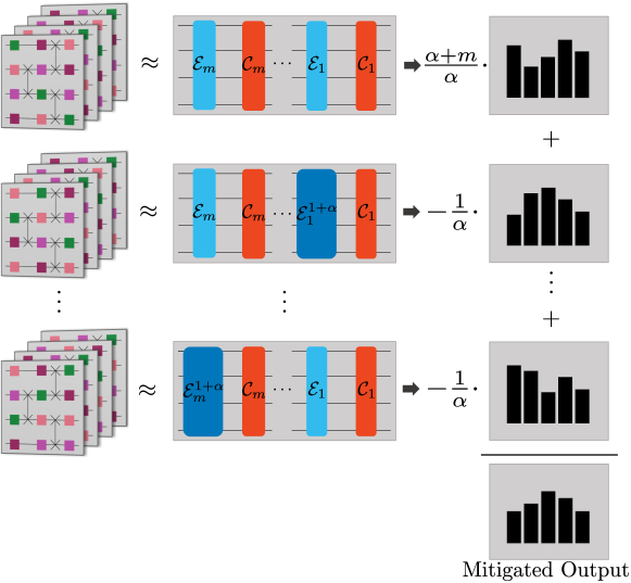
Figure 4: Overview of the NOX+RC procedure. The application circuit is run jointly with a family of noise-amplified versions of itself, each of which is averaged via RC (left). Each set of RC circuits can be approximated (middle) as a sequence of ideal cycles $\mathcal{C}_{i}$ (red) interleaved with non-amplified $\mathcal{E}_{i}$ (cyan) and amplified Pauli stochastic error channels $\mathcal{E}_{i}^{1+\alpha}$ (dark blue). The individual distributions of the original and of each error-amplified RC circuit (right) are used to calculate a mitigated expectation value of a given observable $O$ according to Eq. 13.

V Experimental Results and Analysis

The implementation of the NOX protocol was run on the superconducting IBM quantum hardware platforms ibmq_kolkata, ibmq_guadalupe and ibmq_montreal. This section describes the experimental results and analysis using ibmq_kolkata data. The same analysis was also conducted with both the ibmq_guadalupe and ibmq_montreal data, The full set of results for all three platforms are summarized in Table 5.

V.1 The $\Delta R_{-}(t)$ calculations

The project targeted qubits 19, 20, 22, and 25 on the 27-qubit ibmq_kolkata quantum hardware platform. In post-processing, we examined the effects of each error mitigation procedure mentioned in Section IV on the real-time evolution and calculation of the scattering phase shift.

The first analysis of the ibmq_kolkata data using combinations of these error mitigation procedures is shown in Fig. 5. This figure plots $\Delta R_{-}(t)$, defined as the deviation of the measured $R_{-}(t)$ from the ideal normalized reflection probability at evolution time $t$, for both the unmitigated data and the data obtained after applying the RC+RCAL error mitigation protocols.

We computed the unmitigated data for the free and interacting cases by individually selecting the 30 RC equivalent circuits used to calculate $R_{-}(t)$ at each Trotter time step. We then computed and plotted the 30 $\Delta R_{-}(t)$ data points at each time step and connected them to form 30 curves. Next, we computed and plotted $\Delta R_{-}(t)$ obtained after applying the RC+RCAL protocols for the free and interacting cases. The results for $\Delta R_{-}(t)$ versus $t$ are shown for both the free Fig. 5(a) and interacting cases Fig. 5(b). Comparing $\Delta R_{-}(t)$ obtained with and without mitigation protocols demonstrates the effectiveness of the combined RC+RCAL mitigation over unmitigated data.

The next analysis of the ibmq_kolkata data applies the NOX procedure described in Section IV.2 and Section IV.3. As discussed in Section IV.2, applying NOX requires adding $m+1$ additional circuits to the computation, corresponding to the number of hard cycles in the application circuit.

Each of the circuit components described in Section II contributes to the total number of hard cycles. There is one hard cycle in the state preparation component of the circuit that remains constant for every Trotter step of the simulation. The QFTr circuit component, by itself, consists of twelve hard gate cycles. However, the transpilation optimization reduces this hard cycles count down to eight and also remains a constant factor for each Trotter step. A single Trotter time step in our application requires six two-qubit entangling gates Gustafson et al. (2021). During transpilation, this two-qubit gate count is reduced from six to four. Therefore, Trotter step one requires a total hard cycle count of 13. Each subsequent Trotter step adds an 4 additional hard cycles. We implemented a total of seven Trotter steps. Therefore, the total number $m$ of hard gate cycles in our circuits as we perform the Trotterization from steps one to seven ranged from 13 to 37, covering a wide scope of circuit failure rates.

In addition to these $m$ circuits, we include the original non-amplified circuit to analyze a total of $m+1$ circuits for each Trotter time step. The total number of circuits was sufficiently large that our experiments had to be batched in multiple jobs and effectively run on the cloud over many hours.

We analyzed the NOX procedure by computing $\Delta R_{-}(t)$ obtained using NOX without applying RC and comparing it to values obtained using RC+RCAL and NOX+RC+RCAL. This set of computations illustrates the significant improvement by combining NOX with the original RC+RCAL error mitigation. As expected, the unmitigated results are amplified by NOX, and the values of $\Delta R_{-}(t)$ are larger than the unmitigated values alone. This is because the NOX procedure amplifies the unmitigated values shown in Fig. 5 without the effects of RC present.

Normally, one would perform RC on those $m+1$ circuits and combine the $m+1$ RC averaged circuits using Eq. 13 to compute the data point for each Trotter time-step. However, to compare NOX without RC, we batched the $30(m+1)$ circuits into 30 sets of circuits and then used Eq. 13 to get 30 expectation values for $R_{-}(t)$ for each Trotter step. We then compute the 30 $\Delta R_{-}(t)$ data points for each Trotter step to generate the 30 curves labeled NOX without RC and plotted them in Fig. 6.

We then compute $\Delta R_{-}(t)$ for the entire time evolution after applying the NOX+RC+RCAL protocols and include these curves in Fig. 6. In addition, the RC+RCAL values from Fig. 5 are re-plotted over the entire time evolution. This set of data is plotted for both the free (Fig. 6(a)) and the interacting cases (Fig. 6(b)). These graphs show that although the NOX procedure initially amplifies the unmitigated results and appears to make the error mitigation worse, the addition of NOX to RC+RCAL delivers an overall improved error mitigated result for $\Delta R_{-}(t)$ over the entire time evolution as compared to only applying RC+RCAL.

These results clearly illustrate that the NOX method implemented alone without any additional mitigation did not show dramatic improvements in the $R_{-}(t)$ measurements. However, when the NOX method was combined with RC+RCAL, the final result improved upon just the RC+RCAL. This NOX+RC+RCAL combined error suppression provided the best error mitigation for having the measured data most closely follow the ideal evolution of $R_{-}(t)$ versus t and provided the highest accuracy among the methods tested when calculating $R_{-}(t)$.

The next analysis of the ibmq_kolkata data plotted $\Delta R_{-}(t)$ versus t for the full Trotter evolution for each mitigation procedure in Fig. 7. The graph clearly shows that for both the free (Fig. 7(a)) and interacting (Fig. 7(b)) cases, the NOX+RC+RCAL computations have smaller differences between the measured and ideal values than the RC+RCAL or the original unmitigated data. This set of graphs provides additional evidence that the NOX+RC+RCAL error mitigation significantly improves the computation of $R_{-}(t)$ versus t.

The ibmq_kolkata data was next analyzed by plotting the normalized reflection probabilities versus $t$ for each mitigation procedure. The results are plotted in Fig. 8. For both the free and interacting cases, the plots of the RC+RCAL data showed some improvement compared to the unmitigated data. The combination of NOX+RC+RCAL showed substantial improvement in the results above and beyond the RC+RCAL error mitigation.

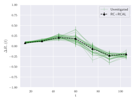
(a) free case

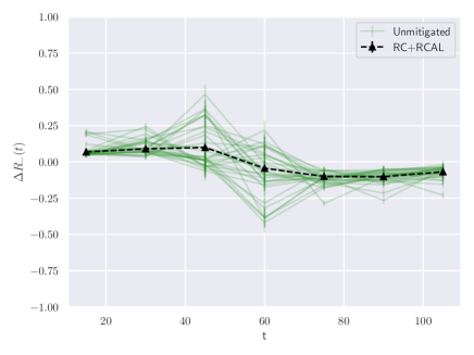
(b) interacting case

Figure 5: Difference in measured $R_{-}(t)$ from the ideal results versus the time evolution for the ibmq_kolkata unmitigated data and with RC+RCAL applied to both the free and interacting cases

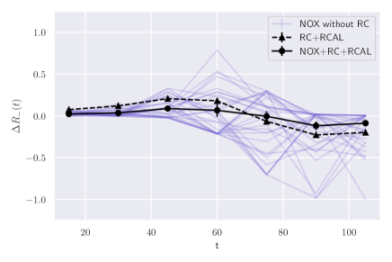
(a) free case

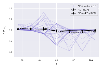
(b) interacting case

Figure 6: Difference in $R_{-}(t)$ from the ideal results versus the time evolution for NOX without RC, RC+RCAL, and NOX+RC+RCAL using the ibmq_kolkata data

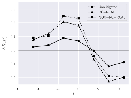
(a) free case

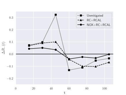
(b) interacting case

Figure 7: Graph of difference between computed $R_{-}(t)$ and the ideal value versus trotter time step for unmitigated, RC+RCAL, and NOX+RC+RCAL ibmq_kolkata free and interacting cases

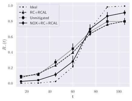
(a) free case

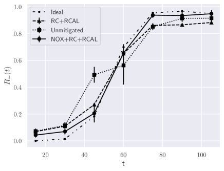
(b) interacting case

Figure 8: ibmq_kolkata normalized reflection probabilities for the free and interacting cases for the ideal, unmitigated, RC+RCAL and NOX+RC+RCAL computations. For both the free and interacting cases NOX combined with RC+RCAL showed substantial improvement to bring the ibmq_kolkata $R_{-}t$ computations into close alignment with the ideally computed values.

We observed that the NOX values appear to be overestimated in the $\tilde{t}^{*}$ region where the $\Delta R_{-}(t)$ is changing rapidly. We computed the ideal numerical calculations for $1/(P_{+}+P_{-})$ in the free and interacting cases as shown in Figs. 9(a) and 9(b). We noticed that empirically that large values of $1/(P_{+}+P_{-})$ appear to be correlated with significant over estimations of the NOX errors. The peaks of $1/(P_{+}+P_{-})$, the change of slope in the graph and the largest error over estimations appear near the values of $\tilde{t}^{*}$ which have values of approximately 69 in the free case and 55 in the interacting case Gustafson et al. (2021).

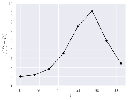
(a) Inverse probability, free case

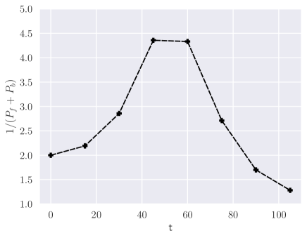
(b) Inverse probability, interacting case

Figure 9: Ideal numerical calculations for $1/(P_{+}+P_{-})$ in the free and interacting cases.

V.2 Metrics

To better quantify these observations, we introduce two metrics to define the closeness of the experimental results compared to the expected values:

$$M_{1}(\{Q_{i,j}\})=\frac{1}{N}\sum_{i=1}^{N}\left(\frac{1}{7}\sum_{j=1}^{7}|Q_{i,j}-I_{j}|\right)$$ (19)

and

$$M_{2}(\{Q_{i,j}\})=\sqrt{\frac{1}{7N}\sum_{i=1}^{N}\sum_{j=1}^{7}(Q_{i,j}-I_{j})^{2}},$$ (20)

where $I_{j}$ represents the ideal Trotterization $R_{-}(t)$ values at Trotter step $j$ and $Q_{i,j}$ represents the measured $R_{-}(t)$ values at Trotter step $j$ at the $i^{th}$ experimental run. Referencing the post-processing analysis procedure in Section V.1, note that $N=30$ total experimental runs for the unmitigated case and $N=1$ experimental runs for the NOX+RC+RCAL and RC+RCAL cases.

The values for these metrics obtained using the ibmq_kolkata hardware platform are shown in Table 5. The table shows that, for ibmq_kolkata, the error reduction using M₁ is $61.05\%$ for the free case and $73.19\%$ for the interacting case. The $M_{2}$ metrics signal a similar improvement ($58.93\%$ for the free case and $75.28\%$ for the interacting case).

The full analysis using these metrics was repeated for the data collected on the IBM quantum hardware platforms ibmq_guadalupe and ibmq_manila. For the 16-qubit ibmq_guadalupe device, we targeted qubits 7, 10, 12, 15, and on the 5-qubit ibmq_manila device, we targeted qubits labeled 0, 1, 2, 3. The results from the analysis of the ibmq_guadalupe data are shown in Table 5 and the ibmq_manila data is shown in Table 5.

We find that, across each device, the NOX data is consistently closer to the ideal values than the unmitigated data, although the total error reduction varies by device. The metrics obtained from the ibmq_kolkata data show the greatest error reduction compared to the other two devices. This is expected because both ibmq_guadalupe and ibmq_manila were older less efficient processors compared to ibmq_kolkata. It is also noted that the interacting cases in each set of experiments show the largest improvement in the $M_{1}$ and $M_{2}$ metrics overall.

[] Metric NOX+RC+RCAL RC+RCAL Unmit. $\frac{\text{NOX+RC+RCAL}}{\text{Unmit.}}$ $\frac{\text{RC+RCAL}}{\text{Unmit.}}$ $(1-\frac{\text{NOX+RC+RCAL}}{\text{Unmit.}})\times 100$ $M_{1}$ (free) $0.061(17)$ $0.153(2)$ $0.167(3)$ 0.363(100) 0.920(20) 63.7 $M_{2}$ (free) $0.071(17)$ $0.165(2)$ $0.187(3)$ 0.382(93) 0.883(18) 61.8 $M_{1}$ (interacting) $0.033(15)$ $0.082(2)$ $0.107(2)$ 0.306(143) 0.764(20) 69.4 $M_{2}$ (interacting) $0.036(16)$ $0.084(2)$ $0.135(2)$ 0.267(117) 0.627(16) 73.3 Metric NOX+RC+RCAL RC+RCAL Unmit. $\frac{\text{NOX+RC+RCAL}}{\text{Unmit.}}$ $\frac{\text{RC+RCAL}}{\text{Unmit.}}$ $(1-\frac{\text{NOX+RC+RCAL}}{\text{Unmit.}})\times 100$ $M_{1}$ (free) $0.102(15)$ $0.172(3)$ $0.194(2)$ 0.527(78) 0.885(17) 47.3 $M_{2}$ (free) $0.115(18)$ $0.181(3)$ $0.211(3)$ 0.543(86) 0.858(16) 45.7 $M_{1}$ (interacting) $0.053(12)$ $0.116(2)$ $0.142(2)$ 0.373(84) 0.815(16) 62.7 $M_{2}$ (interacting) $0.058(13)$ $0.120(2)$ $0.156(2)$ 0.372(82) 0.768(15) 62.8 Metric NOX+RC+RCAL RC+RCAL Unmit. $\frac{\text{NOX+RC+RCAL}}{\text{Unmit.}}$ $\frac{\text{RC+RCAL}}{\text{Unmit.}}$ $(1-\frac{\text{NOX+RC+RCAL}}{\text{Unmit.}})\times 100$ $M_{1}$ (free) $0.205(6)$ $0.258(2)$ $0.275(2)$ 0.745(24) 0.939(12) 25.5 $M_{2}$ (free) $0.230(7)$ $0.268(3)$ $0.295(3)$ 0.779(25) 0.909(12) 22.1 $M_{1}$ (interacting) $0.113(7)$ $0.159(2)$ $0.204(2)$ 0.557(33) 0.779(1) 44.3 $M_{2}$ (interacting) $0.124(6)$ $0.164(2)$ $0.218(2)$ 0.571(30) 0.751(10) 43.9

Table 2: ibmq_kolkata

Table 3: ibmq_guadalupe

Table 4: ibmq_manila

Table 5: Metrics $M_{1}$ and $M_{2}$ calculated for free and interacting cases on three, superconducting IBM Quantum devices: ibmq_kolkata, ibmq_guadalupe, and ibmq_manila.

V.3 Wigner $\Delta{t}$ phase shift calculation

The next analysis of the ibmq_kolkata data focused on calculating the Wigner $\Delta{t}$ phase shift. The results from the reflection probability measurements using the NOX+RC+RCAL error mitigation protocol can be directly applied to the calculation of the phase shifts.

It is noted that the NOX+RC+RCAL yields significant error reduction for scattering probabilities $P_{\pm}(t)$ to be in the $|\pm k\rangle$ state for the QIM Gustafson et al. (2021). As discussed in Section II, the normalized reflection probability shown in Eq. 4 allows us to estimate time delays and phase shifts due to interactions.

Following Gustafson et al. (2021), we assume the phase shift follows the empirical sigmoid function shown in Eq. 8. The sigmoid fits obtained using Eq. 8 and the calculation of $\Delta t$ with and without NOX+RC+RCAL error suppression for the free case (Fig. 10a) and interacting case (Fig. 10b) were then computed. The differences of $\tilde{t}^{*}$ give us the time delay between the free and interacting wave packets. We define this difference as $\Delta t$.

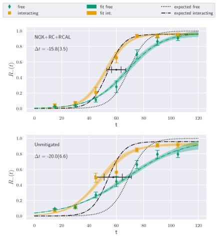
Figure 10: The time evolution and sigmoid fits for the simulation on ibmq_kolkata including the NOX+RC+RCAL error mitigation and with only the unmitigated data.

By calculating and comparing the percentage differences between the experimental results ($\Delta t_{\rm Unmit.}$ and $\Delta t_{\rm NOX}$) and the ideal results, we can see that the accuracy of the $\Delta t_{\rm NOX}$ compared to $\Delta t_{\rm Unmit.}$ has improved by $28.71\%$ and that the error bar has decreased by $63.41\%$. While both results agree with the expected value of $\Delta t=-14.91(52)$, the NOX calculation shrinks the error bands and provides a more precise result. The signs of the differences are similar for the two methods (positive for $t\leq 60$ and negative later). However, the magnitude of these difference are significantly smaller for the NOX procedure. Visually, it is clear that the NOX errors are about twice smaller than the unmitigated errors.

By design, the NOX mitigation technique produces more accurate expectation values for the observables under consideration. These are the $|0100\rangle\langle 0100|$ and $|1000\rangle\langle 1000|$ states corresponding to $\pm k$ momentum states after the Fourier transform. Like other mitigation techniques, NOX trades precision for accuracy but compensates for the loss in precision by increasing the number of circuits and shots. Nonetheless, getting an error bar that adequately represents the precision of the mitigated expectation values remains a challenge because the assumptions underlying NOX (as well as other mitigation techniques) aren’t guaranteed to apply perfectly, which may result in systematic loss of accuracy.

This is likely an artifact that the scattering process is elastic and far from any resonances. Together, these two factors render the scattering process semi-robust to noise, given that the particle does not slosh back and forth within the potential well. In this sense, the time delay $\Delta t$ is a good example of a physical quantity that is robust against computation errors and consequently weakly sensitive to error mitigation. To estimate the time delay due to the interaction, it is very useful to have estimated systematic errors as discussed in Appendix A. This allows a determination of the free parameters using $\chi^{2}$ minimization.

To account for these effective systematic errors, we provide error bars on NOX-mitigated results by adding a systematic heuristic upper-bound to the statistical error bar obtained by taking the magnitude of the NOX correction Eq. 21:

$$\Delta^{\rm sys}_{\rm bound}:=\left|\hat{O}_{\rm NOX+RC}-\hat{O}_{\rm RC}\right|$$ (21)

We point out that this upper bound is often generous for the systems under scope and purposefully overestimates systematic errors. Accurately tightening the systematic error bars of mitigated outcomes for computations vulnerable to non-Markovian or time-dependent noise sources remains an open problem. We expand on the reasoning behind this heuristic in the Supplemental Material in Appendix A.

VI Summary

We improved the previous real-time scattering calculations by applying three compounding error suppression techniques: RCAL, RC and NOX. These improvements are applicable and can be implemented across a spectrum of STEM application domains. For a wide range of circuit depths and on three different devices, we consistently observed noticeable error reductions from NOX alone on top of the error reduction provided by RC and RCAL. However, the sensitivity to improved error mitigation results will likely be observable dependent. This improved accuracy for our proof-of-concept application circuits demonstrated the applicability of NOX on cloud platforms, in the advent where circuits are executed in substantially time-separated batches. We further supplemented our mitigated results with systematic error bars that accounted for unmitigated errors. Future work is planned for further refinement of systematic errors.

We also note crucial differences between the NOX protocol and other noise extrapolation methods based on RIIM He et al. (2020). Although both RIIM and NOX implement similar approaches, the RIIM protocol targets individual cX gates. Because RIIM is a noise-agnostic method, it cannot correctly amplify noise processes that do not commute with the cX gates. NOX is a more noise-aware version of the standard RIIM noise extrapolation techniques. NOX targets entire gate cycles affected by various non-local and non-depolarising noise processes. NOX, therefore, provides a broader error suppression context that enables more accurate amplification of noise processes than methods that only focus on individual gates.

VII Competing interests

A. C-D. has a financial interest in Keysight Technology Inc. and the use of True-Q software Beale et al. (2020). The remaining authors declare no competing interests.

VIII Data Availability

Data is available from the corresponding author upon reasonable request.

Supplementary Material

Appendix A Error Estimation Using Noiseless Output Extrapolation

As shown in the previous section, NOX ideally induces a first-order correction on the output. However, this mitigation effect is founded around a Markovian time-independent error model, as well as on a perfect error amplification $\mathcal{E}_{i}\rightarrow\mathcal{E}_{i}^{1+\alpha}$ through cycle repetition. A number of physical mechanisms can bring us outside of this framework, and reduce the accuracy of NOX-mitigated results.

For instance, one mechanism in which accuracy can be lost is if an error channel $\mathcal{E}_{i}$ doesn’t exactly commute with the cycle $C_{i}$. In this case, the amplified error resulting from repeating $\pazocal{E}_{i}^{\rm amp}=C_{i}^{-(1+\alpha)}\left(\mathcal{E}_{i}C_{i}\right)^{1+\alpha}$, might slightly differ from the amplified channel $\pazocal{E}_{i}^{1+\alpha}$. Other mechanisms for systematic loss in accuracy include time-dependent effects such as error drift and re-calibration, as well as non-Markovian effects.

To account for these effective systematic errors, we provide error bars on NOX-mitigated results by adding a systematic heuristic upper-bound to the statistical error bar obtained by taking the magnitude of the NOX correction:

$$\Delta^{\rm sys}_{\rm bound}:=\left|\hat{O}_{\rm RC+NOX}-\hat{O}_{\rm RC}\right|\leavevmode\nobreak\ .$$ (22)

To see the reasoning behind this choice of upper bound, recall LABEL:{eq:nox_delta_horder}. To accommodate for faulty error amplification mechanisms, we modify LABEL:{eq:nox_delta_horder} by adding new terms:

$$\langle\mathcal{C}_{i}\rangle_{\rm RC}=\mathcal{C}_{\rm ideal}+\alpha\Delta_{i}+\alpha\Delta^{(1)}_{i}+\Delta^{(2)}_{i}+\sum_{j=1}^{m}\Delta_{j}+h.o.$$ (23)

Here the term $\alpha\Delta^{(1)}_{i}$ would represent the effect of a systematic fluctuation in the amplification mechanism; the $\Delta^{(2)}_{i}$ term would instead correspond to systematic fluctuations in non-amplified error components due to e.g time-dependent effects arising between circuits. By substituting  Eq. 23 into  Eq. 13 we obtain

$$\hat{O}_{\rm RC+NOX}=\hat{O}_{\rm ideal}-\sum_{i}\mathbb{E}\left(O\Bigg{|}\Delta_{i}^{(1)}+\frac{\Delta^{(2)}_{i}}{\alpha}\right)+h.o.$$ (24)

where the higher order terms are of second order in the circuit error probability. Let’s define the following error ratio

$$\Gamma:=\frac{\left|\sum_{i}\mathbb{E}\left(O|\Delta_{i}\right)\right|}{\left|\sum_{i}\mathbb{E}\left(O\Bigg{|}\Delta_{i}^{(1)}+\frac{\Delta^{(2)}_{i}}{\alpha}\right)\right|}$$ (25)

The numerator is the first-order error term meant to be removed by NOX. The denominator is zero in the absence of violations to the framework that led to LABEL:{eq:nox_delta_horder}. With the expectation of weak violations (weaker than the “baseline” noise induced by $\Delta_{i}$ ) we certainly expect $\Gamma$ to be greater than 1. Here, we consider the eventuality that the effect of leftover error $\sum_{i}\Delta_{i}^{(1)}+\frac{\Delta^{(2)}_{i}}{\alpha}$ on the observable $O$ is at least comparable to the effect of the first order unmitigated error $\sum_{i}\Delta_{i}$. That is, instead of assuming $\Gamma\gg 1$ (which holds when there are close to no violations of the assumptions that led to LABEL:{eq:nox_delta_horder}) we make the much more cautious assumption $\Gamma\geq 2$. In other words, we assume that effects such as imperfect averaging due to time-dependent error rate fluctuations aren’t necessarily negligible, but are at least twice smaller than baseline error rates. From there, we get our first-order upper bound on the systematic error in NOX:

$$\left|\hat{O}_{\rm RC+NOX}-\hat{O}_{\rm RC}\right|\simeq\left|\sum_{i}\mathbb{E}\left(O\Bigg{|}\Delta_{i}-\Delta_{i}^{(1)}-\frac{\Delta^{(2)}_{i}}{\alpha}\right)\right|$$ (Eq. 13, Section IV.3, Eq. 23)

$$\geq\left|\left|\sum_{i}\mathbb{E}(O|\Delta_{i})\right|-\left|\sum_{i}\mathbb{E}\left(O\Big{|}\Delta_{i}^{(1)}+\frac{\Delta^{(2)}_{i}}{\alpha}\right)\right|\right|$$ (rev. triang. ineq.)

$$=|\Gamma-1|\left|\sum_{i}\mathbb{E}\left(O\Big{|}\Delta_{i}^{(1)}+\frac{\Delta^{(2)}_{i}}{\alpha}\right)\right| \Gamma$$ (def. of , Eq. 25)

$$\geq\left|\sum_{i}\mathbb{E}\left(O\Big{|}\Delta_{i}^{(1)}+\frac{\Delta^{(2)}_{i}}{\alpha}\right)\right|\leavevmode\nobreak\ . \Gamma\geq 2$$ (Assumption )

Note that the assumption $\Gamma\geq 2$ is coarse and inspired by empirical data. (see Fig. 11). Refining device-specific or application-specific upper bounds on $\Gamma$ is left as an open research avenue.

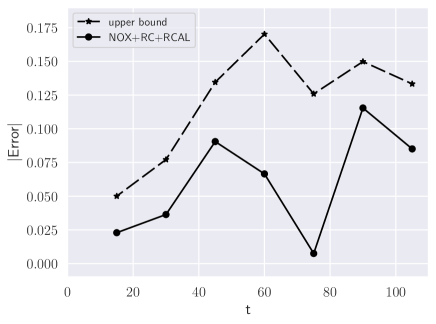
(a) free case

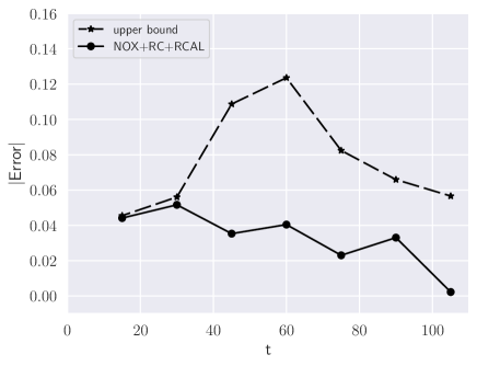
(b) interacting case

Figure 11: Actual (solid line, circles) and heuristic upper bound (dashed line, stars) on NOX errors for calculated $R_{-}(t)$ values in absolute value for ibmq_kolkata in the free and interacting cases.

References

- Alam et al. (2022) M. S. Alam, S. Belomestnykh, N. Bornman, G. Cancelo, Y.-C. Chao, M. Checchin, V. S. Dinh, A. Grassellino, E. J. Gustafson, R. Harnik, C. R. H. McRae, Z. Huang, K. Kapoor, T. Kim, J. B. Kowalkowski, M. J. Kramer, Y. Krasnikova, P. Kumar, D. M. Kurkcuoglu, H. Lamm, A. L. Lyon, D. Milathianaki, A. Murthy, J. Mutus, I. Nekrashevich, J. Oh, A. B. Özgüler, G. N. Perdue, M. Reagor, A. Romanenko, J. A. Sauls, L. Stefanazzi, N. M. Tubman, D. Venturelli, C. Wang, X. You, D. M. T. van Zanten, L. Zhou, S. Zhu, and S. Zorzetti, “Quantum computing hardware for hep algorithms and sensing,” (2022).
- Bauer et al. (2022) C. W. Bauer, Z. Davoudi, A. B. Balantekin, T. Bhattacharya, M. Carena, W. A. de Jong, P. Draper, A. El-Khadra, N. Gemelke, M. Hanada, D. Kharzeev, H. Lamm, Y.-Y. Li, J. Liu, M. Lukin, Y. Meurice, C. Monroe, B. Nachman, G. Pagano, J. Preskill, E. Rinaldi, A. Roggero, D. I. Santiago, M. J. Savage, I. Siddiqi, G. Siopsis, D. Van Zanten, N. Wiebe, Y. Yamauchi, K. Yeter-Aydeniz, and S. Zorzetti, “Quantum simulation for high energy physics,” (2022).
- Humble et al. (2022) T. S. Humble, A. Delgado, R. Pooser, C. Seck, R. Bennink, V. Leyton-Ortega, C. C. J. Wang, E. Dumitrescu, T. Morris, K. Hamilton, D. Lyakh, P. Date, Y. Wang, N. A. Peters, K. J. Evans, M. Demarteau, A. McCaskey, T. Nguyen, S. Clark, M. Reville, A. Di Meglio, M. Grossi, S. Vallecorsa, K. Borras, K. Jansen, and D. Krücker, “Snowmass white paper: Quantum computing systems and software for high-energy physics research,” (2022).
- Klco et al. (2022) N. Klco, A. Roggero, and M. J. Savage, Rept. Prog. Phys. 85, 064301 (2022), arXiv:2107.04769 [quant-ph] .
- Bañuls and Cichy (2020) M. C. Bañuls and K. Cichy, Rept. Prog. Phys. 83, 024401 (2020), arXiv:1910.00257 [hep-lat] .
- Bañuls et al. (2020) M. C. Bañuls et al., Eur. Phys. J. D 74, 165 (2020), arXiv:1911.00003 [quant-ph] .
- Georgescu et al. (2014) I. M. Georgescu, S. Ashhab, and F. Nori, Rev. Mod. Phys. 86, 153 (2014).
- Cervera-Lierta (2018) A. Cervera-Lierta, Quantum 2, 114 (2018).
- Lamm and Lawrence (2018) H. Lamm and S. Lawrence, Phys. Rev. Lett. 121, 170501 (2018), arXiv:1806.06649 [quant-ph] .
- Gustafson et al. (2019a) E. Gustafson, Y. Meurice, and J. Unmuth-Yockey, Physical Review D 99 (2019a), 10.1103/PhysRevD.99.094503.
- Gustafson et al. (2019b) E. Gustafson, P. Dreher, Z. Hang, and Y. Meurice, “Benchmarking quantum computers for real-time evolution of a field theory with error mitigation,” (2019b), arXiv:1910.09478 [hep-lat] .
- Kim et al. (2020) M. Kim, Y. Song, J. Kim, and J. Ahn, PRX Quantum 1 (2020), 10.1103/prxquantum.1.020323.
- Yeter-Aydeniz et al. (2021) K. Yeter-Aydeniz, G. Siopsis, and R. C. Pooser, “Scattering in the ising model using quantum lanczos algorithm,” (2021), arXiv:2008.08763 [quant-ph] .
- Vovrosh and Knolle (2020) J. Vovrosh and J. Knolle, (2020), arXiv:2001.03044 [cond-mat.str-el] .
- Salathé et al. (2015) Y. Salathé, M. Mondal, M. Oppliger, J. Heinsoo, P. Kurpiers, A. Potočnik, A. Mezzacapo, U. Las Heras, L. Lamata, E. Solano, and et al., Physical Review X 5 (2015), 10.1103/physrevx.5.021027.
- Tan et al. (2021) W. L. Tan, P. Becker, F. Liu, G. Pagano, K. S. Collins, A. De, L. Feng, H. B. Kaplan, A. Kyprianidis, R. Lundgren, and et al., Nature Physics (2021), 10.1038/s41567-021-01194-3.
- Smith et al. (2019) A. Smith, M. S. Kim, F. Pollmann, and J. Knolle, npj Quantum Information 5 (2019), 10.1038/s41534-019-0217-0.
- Labuhn et al. (2016) H. Labuhn, D. Barredo, S. Ravets, S. de Léséleuc, T. Macrì, T. Lahaye, and A. Browaeys, Nature 534, 667–670 (2016).
- Zhang et al. (2017) J. Zhang, G. Pagano, P. W. Hess, A. Kyprianidis, P. Becker, H. Kaplan, A. V. Gorshkov, Z. X. Gong, and C. Monroe, Nature (London) 551, 601 (2017), arXiv:1708.01044 [quant-ph] .
- Kadowaki and Nishimori (1998) T. Kadowaki and H. Nishimori, Phys. Rev. E 58, 5355 (1998).
- Bernien et al. (2017) H. Bernien, S. Schwartz, A. Keesling, H. Levine, A. Omran, H. Pichler, S. Choi, A. S. Zibrov, M. Endres, M. Greiner, V. Vuletić, and M. D. Lukin, Nature (London) 551, 579 (2017), arXiv:1707.04344 [quant-ph] .
- Ciavarella et al. (2022) A. N. Ciavarella, S. Caspar, H. Singh, M. J. Savage, and P. Lougovski, (2022), arXiv:2207.09438 [quant-ph] .
- Alexandru et al. (2019a) A. Alexandru, P. F. Bedaque, S. Harmalkar, H. Lamm, S. Lawrence, and N. C. Warrington, Physical Review D 100 (2019a), 10.1103/physrevd.100.114501.
- Zohar et al. (2013a) E. Zohar, J. I. Cirac, and B. Reznik, Physical Review A 88 (2013a), 10.1103/physreva.88.023617.
- Martinez et al. (2016) E. A. Martinez, C. A. Muschik, P. Schindler, D. Nigg, A. Erhard, M. Heyl, P. Hauke, M. Dalmonte, T. Monz, P. Zoller, and R. Blatt, Nature 534, 516 EP (2016).
- Buyens et al. (2017) B. Buyens, J. Haegeman, F. Hebenstreit, F. Verstraete, and K. Van Acoleyen, Phys. Rev. D 96, 114501 (2017), arXiv:1612.00739 [hep-lat] .
- Jahin et al. (2022) A. Jahin, A. C. Y. Li, T. Iadecola, P. P. Orth, G. N. Perdue, A. Macridin, M. S. Alam, and N. M. Tubman, Physical Review A 106 (2022), 10.1103/physreva.106.022434.
- Klco et al. (2018) N. Klco, E. F. Dumitrescu, A. J. McCaskey, T. D. Morris, R. C. Pooser, M. Sanz, E. Solano, P. Lougovski, and M. J. Savage, Phys. Rev. A98, 032331 (2018), arXiv:1803.03326 [quant-ph] .
- Brower et al. (2019) R. C. Brower, D. Berenstein, and H. Kawai, PoS LATTICE2019, 112 (2019), arXiv:2002.10028 [hep-lat] .
- Karpov et al. (2020) P. I. Karpov, G. Y. Zhu, M. P. Heller, and M. Heyl, (2020), arXiv:2011.11624 [cond-mat.quant-gas] .
- Holland et al. (2020) E. T. Holland, K. A. Wendt, K. Kravvaris, X. Wu, W. E. Ormand, J. L. DuBois, S. Quaglioni, and F. Pederiva, Physical Review A 101 (2020), 10.1103/physreva.101.062307.
- Roggero et al. (2020) A. Roggero, C. Gu, A. Baroni, and T. Papenbrock, Physical Review C 102 (2020), 10.1103/physrevc.102.064624.
- Surace and Lerose (2021) F. M. Surace and A. Lerose, (2021), arXiv:2011.10583 [cond-mat.quant-gas] .
- Kharzeev and Kikuchi (2020) D. E. Kharzeev and Y. Kikuchi, Phys. Rev. Res. 2, 023342 (2020), arXiv:2001.00698 [hep-ph] .
- Ikeda et al. (2020) K. Ikeda, D. E. Kharzeev, and Y. Kikuchi, (2020), arXiv:2012.02926 [hep-ph] .
- Briceño et al. (2021) R. A. Briceño, J. V. Guerrero, M. T. Hansen, and A. M. Sturzu, Phys. Rev. D 103, 014506 (2021), arXiv:2007.01155 [hep-lat] .
- Van Damme et al. (2021) M. Van Damme, L. Vanderstraeten, J. De Nardis, J. Haegeman, and F. Verstraete, Phys. Rev. Research 3, 013078 (2021).
- Zohar et al. (2012) E. Zohar, J. I. Cirac, and B. Reznik, Phys. Rev. Lett. 109, 125302 (2012), arXiv:1204.6574 [quant-ph] .
- Zohar et al. (2013b) E. Zohar, J. I. Cirac, and B. Reznik, Phys. Rev. Lett. 110, 125304 (2013b), arXiv:1211.2241 [quant-ph] .
- Zohar et al. (2013c) E. Zohar, J. I. Cirac, and B. Reznik, Phys. Rev. A88, 023617 (2013c), arXiv:1303.5040 [quant-ph] .
- Zohar and Burrello (2015) E. Zohar and M. Burrello, Phys. Rev. D91, 054506 (2015), arXiv:1409.3085 [quant-ph] .
- Zohar et al. (2016) E. Zohar, J. I. Cirac, and B. Reznik, Rept. Prog. Phys. 79, 014401 (2016), arXiv:1503.02312 [quant-ph] .
- Zohar et al. (2017) E. Zohar, A. Farace, B. Reznik, and J. I. Cirac, Phys. Rev. A95, 023604 (2017), arXiv:1607.08121 [quant-ph] .
- Klco et al. (2020) N. Klco, J. R. Stryker, and M. J. Savage, Phys. Rev. D 101, 074512 (2020), arXiv:1908.06935 [quant-ph] .
- Ciavarella et al. (2021) A. Ciavarella, N. Klco, and M. J. Savage, “A Trailhead for Quantum Simulation of SU(3) Yang-Mills Lattice Gauge Theory in the Local Multiplet Basis,” (2021), arXiv:2101.10227 [quant-ph] .
- Bender et al. (2018) J. Bender, E. Zohar, A. Farace, and J. I. Cirac, New J. Phys. 20, 093001 (2018), arXiv:1804.02082 [quant-ph] .
- Liu and Xin (2020) J. Liu and Y. Xin, “Quantum simulation of quantum field theories as quantum chemistry,” (2020), arXiv:2004.13234 [hep-th] .
- Hackett et al. (2019) D. C. Hackett, K. Howe, C. Hughes, W. Jay, E. T. Neil, and J. N. Simone, Phys. Rev. A 99, 062341 (2019), arXiv:1811.03629 [quant-ph] .
- Alexandru et al. (2019b) A. Alexandru, P. F. Bedaque, S. Harmalkar, H. Lamm, S. Lawrence, and N. C. Warrington (NuQS), Phys.Rev.D 100, 114501 (2019b), arXiv:1906.11213 [hep-lat] .
- Yamamoto (2021) A. Yamamoto, PTEP 2021, 013B06 (2021), arXiv:2008.11395 [hep-lat] .
- Haase et al. (2021) J. F. Haase, L. Dellantonio, A. Celi, D. Paulson, A. Kan, K. Jansen, and C. A. Muschik, Quantum 5, 393 (2021), arXiv:2006.14160 [quant-ph] .
- Armon et al. (2021) T. Armon, S. Ashkenazi, G. García-Moreno, A. González-Tudela, and E. Zohar, “Photon-mediated Stroboscopic Quantum Simulation of a Lattice Gauge Theory,” (2021), arXiv:2107.13024 [quant-ph] .
- Bazavov et al. (2019) A. Bazavov, S. Catterall, R. G. Jha, and J. Unmuth-Yockey, Phys. Rev. D 99, 114507 (2019).
- Bazavov et al. (2015) A. Bazavov, Y. Meurice, S.-W. Tsai, J. Unmuth-Yockey, and J. Zhang, Phys. Rev. D92, 076003 (2015), arXiv:1503.08354 [hep-lat] .
- Zhang et al. (2018) J. Zhang, J. Unmuth-Yockey, J. Zeiher, A. Bazavov, S. W. Tsai, and Y. Meurice, Phys. Rev. Lett. 121, 223201 (2018), arXiv:1803.11166 [hep-lat] .
- Unmuth-Yockey et al. (2018) J. Unmuth-Yockey, J. Zhang, A. Bazavov, Y. Meurice, and S.-W. Tsai, Phys. Rev. D98, 094511 (2018), arXiv:1807.09186 [hep-lat] .
- Unmuth-Yockey (2019) J. F. Unmuth-Yockey, Phys. Rev. D 99, 074502 (2019), arXiv:1811.05884 [hep-lat] .
- Kreshchuk et al. (2020a) M. Kreshchuk, W. M. Kirby, G. Goldstein, H. Beauchemin, and P. J. Love, “Quantum Simulation of Quantum Field Theory in the Light-Front Formulation,” (2020a), arXiv:2002.04016 [quant-ph] .
- Kreshchuk et al. (2020b) M. Kreshchuk, S. Jia, W. M. Kirby, G. Goldstein, J. P. Vary, and P. J. Love, “Simulating Hadronic Physics on NISQ devices using Basis Light-Front Quantization,” (2020b), arXiv:2011.13443 [quant-ph] .
- Raychowdhury and Stryker (2018) I. Raychowdhury and J. R. Stryker, “Solving Gauss’s Law on Digital Quantum Computers with Loop-String-Hadron Digitization,” (2018), arXiv:1812.07554 [hep-lat] .
- Raychowdhury and Stryker (2020) I. Raychowdhury and J. R. Stryker, Phys. Rev. D 101, 114502 (2020), arXiv:1912.06133 [hep-lat] .
- Davoudi et al. (2020) Z. Davoudi, I. Raychowdhury, and A. Shaw, “Search for Efficient Formulations for Hamiltonian Simulation of non-Abelian Lattice Gauge Theories,” (2020), arXiv:2009.11802 [hep-lat] .
- Wiese (2014) U.-J. Wiese, Proceedings, 24th International Conference on Ultra-Relativistic Nucleus-Nucleus Collisions (Quark Matter 2014): Darmstadt, Germany, May 19-24, 2014, Nucl. Phys. A931, 246 (2014), arXiv:1409.7414 [hep-th] .
- Luo et al. (2019) D. Luo, J. Shen, M. Highman, B. K. Clark, B. DeMarco, A. X. El-Khadra, and B. Gadway, “A Framework for Simulating Gauge Theories with Dipolar Spin Systems,” (2019), arXiv:1912.11488 [quant-ph] .
- Mathis et al. (2020) S. V. Mathis, G. Mazzola, and I. Tavernelli, Phys. Rev. D 102, 094501 (2020), arXiv:2005.10271 [quant-ph] .
- Singh (2019) H. Singh, “Qubit nonlinear sigma models,” (2019), arXiv:1911.12353 [hep-lat] .
- Singh and Chandrasekharan (2019) H. Singh and S. Chandrasekharan, Phys. Rev. D 100, 054505 (2019), arXiv:1905.13204 [hep-lat] .
- Buser et al. (2020) A. J. Buser, T. Bhattacharya, L. Cincio, and R. Gupta, “Quantum simulation of the qubit-regularized O(3)-sigma model,” (2020), arXiv:2006.15746 [quant-ph] .
- Bhattacharya et al. (2020) T. Bhattacharya, A. J. Buser, S. Chandrasekharan, R. Gupta, and H. Singh, “Qubit regularization of asymptotic freedom,” (2020), arXiv:2012.02153 [hep-lat] .
- Barata et al. (2020) J. a. Barata, N. Mueller, A. Tarasov, and R. Venugopalan, “Single-particle digitization strategy for quantum computation of a scalar field theory,” (2020), arXiv:2012.00020 [hep-th] .
- Kreshchuk et al. (2020c) M. Kreshchuk, S. Jia, W. M. Kirby, G. Goldstein, J. P. Vary, and P. J. Love, “Light-Front Field Theory on Current Quantum Computers,” (2020c), arXiv:2009.07885 [quant-ph] .
- Ji et al. (2020) Y. Ji, H. Lamm, and S. Zhu (NuQS), Phys. Rev. D 102, 114513 (2020), arXiv:2005.14221 [hep-lat] .
- Bauer and Grabowska (2021) C. W. Bauer and D. M. Grabowska, “Efficient Representation for Simulating U(1) Gauge Theories on Digital Quantum Computers at All Values of the Coupling,” (2021), arXiv:2111.08015 [hep-ph] .
- Gustafson (2021) E. Gustafson, Phys. Rev. D 103, 114505 (2021), arXiv:2104.10136 [quant-ph] .
- Hartung et al. (2022) T. Hartung, T. Jakobs, K. Jansen, J. Ostmeyer, and C. Urbach, Eur. Phys. J. C 82, 237 (2022), arXiv:2201.09625 [hep-lat] .
- Grabowska et al. (2022) D. M. Grabowska, C. Kane, B. Nachman, and C. W. Bauer, “Overcoming exponential scaling with system size in Trotter-Suzuki implementations of constrained Hamiltonians: 2+1 U(1) lattice gauge theories,” (2022), arXiv:2208.03333 [quant-ph] .
- Murairi et al. (2022) E. M. Murairi, M. J. Cervia, H. Kumar, P. F. Bedaque, and A. Alexandru, “How many quantum gates do gauge theories require?” (2022), arXiv:2208.11789 [hep-lat] .
- Gustafson (2022) E. Gustafson, “Noise Improvements in Quantum Simulations of sQED using Qutrits,” (2022), arXiv:2201.04546 [quant-ph] .
- Farrell et al. (2022) R. C. Farrell, I. A. Chernyshev, S. J. M. Powell, N. A. Zemlevskiy, M. Illa, and M. J. Savage, (2022), arXiv:2209.10781 [quant-ph] .
- Gustafson et al. (2022) E. J. Gustafson, H. Lamm, F. Lovelace, and D. Musk, (2022), arXiv:2208.12309 [quant-ph] .
- McDonough et al. (2022) B. McDonough, A. Mari, N. Shammah, N. T. Stemen, M. Wahl, W. J. Zeng, and P. P. Orth, (2022), arXiv:2210.08611 [quant-ph] .
- Chen et al. (2022) I.-C. Chen, B. Burdick, Y. Yao, P. P. Orth, and T. Iadecola, Physical Review Research 4 (2022), 10.1103/physrevresearch.4.043027.
- Gustafson et al. (2021) E. Gustafson, Y. Zhu, P. Dreher, N. M. Linke, and Y. Meurice, Physical Review D 104 (2021), 10.1103/physrevd.104.054507.
- Meurice (2021) Y. Meurice, Quantum field theory: a quantum computation approach (Institute of Physics Publishing, Bristol, 2021).
- Meurice et al. (2020) Y. Meurice, R. Sakai, and J. Unmuth-Yockey, (2020), arXiv:2010.06539 [hep-lat] .
- Temme et al. (2017) K. Temme, S. Bravyi, and J. M. Gambetta, Phys. Rev. Lett. 119, 180509 (2017).
- Ferracin et al. (2022) S. Ferracin, A. Hashim, J.-L. Ville, R. Naik, A. Carignan-Dugas, H. Qassim, A. Morvan, D. I. Santiago, I. Siddiqi, and J. J. Wallman, “Efficiently improving the performance of noisy quantum computers,” (2022), arXiv:2201.10672 [quant-ph] .
- van den Berg et al. (2023) E. van den Berg, Z. K. Minev, A. Kandala, and K. Temme, Nature Physics (2023), 10.1038/s41567-023-02042-2.
- A Rahman et al. (2022) S. A Rahman, R. Lewis, E. Mendicelli, and S. Powell, Phys. Rev. D 106, 074502 (2022).
- Farrell et al. (2023) R. C. Farrell, I. A. Chernyshev, S. J. M. Powell, N. A. Zemlevskiy, M. Illa, and M. J. Savage, Phys. Rev. D 107, 054512 (2023).
- Urbanek et al. (2021) M. Urbanek, B. Nachman, V. R. Pascuzzi, A. He, C. W. Bauer, and W. A. de Jong, Phys. Rev. Lett. 127, 270502 (2021).
- Strikis et al. (2021) A. Strikis, D. Qin, Y. Chen, S. C. Benjamin, and Y. Li, PRX Quantum 2, 040330 (2021).
- McClean et al. (2020) J. R. McClean, Z. Jiang, N. C. Rubin, R. Babbush, and H. Neven, Nature Communications 11, 636 (2020).
- Takeshita et al. (2020) T. Takeshita, N. C. Rubin, Z. Jiang, E. Lee, R. Babbush, and J. R. McClean, Phys. Rev. X 10, 011004 (2020).
- Endo et al. (2018) S. Endo, S. C. Benjamin, and Y. Li, Phys. Rev. X 8, 031027 (2018).
- Kandala et al. (2019) A. Kandala, K. Temme, A. D. Córcoles, A. Mezzacapo, J. M. Chow, and J. M. Gambetta, Nature 567, 491–495 (2019).
- Dumitrescu et al. (2018) E. F. Dumitrescu, A. J. McCaskey, G. Hagen, G. R. Jansen, T. D. Morris, T. Papenbrock, R. C. Pooser, D. J. Dean, and P. Lougovski, Phys. Rev. Lett. 120, 210501 (2018), arXiv:1801.03897 [quant-ph] .
- McCaskey et al. (2019) A. J. McCaskey, Z. P. Parks, J. Jakowski, S. V. Moore, T. D. Morris, T. S. Humble, and R. C. Pooser, npj Quantum Information 5 (2019), 10.1038/s41534-019-0209-0.
- Li and Benjamin (2017) Y. Li and S. C. Benjamin, Physical Review X 7, 021050 (2017).
- Pascuzzi et al. (2022) V. R. Pascuzzi, A. He, C. W. Bauer, W. A. de Jong, and B. Nachman, Phys. Rev. A 105, 042406 (2022).
- Kim et al. (2023a) Y. Kim, C. J. Wood, T. J. Yoder, S. T. Merkel, J. M. Gambetta, K. Temme, and A. Kandala, Nature Physics 19, 752 (2023a).
- Kim et al. (2023b) Y. Kim, A. Eddins, S. Anand, K. X. Wei, E. van den Berg, S. Rosenblatt, H. Nayfeh, Y. Wu, M. Zaletel, K. Temme, and A. Kandala, Nature 618, 500 (2023b).
- He et al. (2020) A. He, B. Nachman, W. A. de Jong, and C. W. Bauer, Phys. Rev. A 102, 012426 (2020).
- Kogut (1983) J. B. Kogut, Rev. Mod. Phys. 55, 775 (1983).
- Wigner (1955) E. P. Wigner, Phys. Rev. 98, 145 (1955).
- Note (1) This relation can be justified from the time-reversal argument that after only half of the phase shift, , has built up while the other half builds after . This is why the total phase shift is historically denoted .
- Bravyi et al. (2021) S. Bravyi, S. Sheldon, A. Kandala, D. C. Mckay, and J. M. Gambetta, Phys. Rev. A 103, 042605 (2021).
- Nation et al. (2021) P. D. Nation, H. Kang, N. Sundaresan, and J. M. Gambetta, PRX Quantum 2, 040326 (2021), arXiv:2108.12518 [quant-ph] .
- Nachman et al. (2020) B. Nachman, M. Urbanek, W. A. de Jong, and C. W. Bauer, npj Quantum Information 6, 84 (2020), arXiv:1910.01969 [quant-ph] .
- Hicks et al. (2021) R. Hicks, C. W. Bauer, and B. Nachman, Phys. Rev. A 103, 022407 (2021).
- Wang et al. (2021) K. Wang, Y.-A. Chen, and X. Wang, “Measurement error mitigation via truncated neumann series,” (2021).
- Geller and Sun (2021) M. R. Geller and M. Sun, Quantum Science and Technology 6, 025009 (2021).
- Maciejewski et al. (2020) F. B. Maciejewski, Z. Zimborás, and M. Oszmaniec, Quantum 4, 257 (2020).
- van den Berg et al. (2022) E. van den Berg, Z. K. Minev, and K. Temme, Physical Review A 105 (2022), 10.1103/physreva.105.032620.
- Wallman and Emerson (2016) J. J. Wallman and J. Emerson, Physical Review A 94 (2016), 10.1103/physreva.94.052325.
- Beale et al. (2020) S. J. Beale, K. Boone, A. Carignan-Dugas, A. Chytros, D. Dahlen, H. Dawkins, J. Emerson, S. Ferracin, V. Frey, I. Hincks, D. Hufnagel, P. Iyer, A. Jain, J. Kolbush, E. Ospadov, J. L. Pino, H. Qassim, J. Saunders, J. Skanes-Norman, A. Stasiuk, J. J. Wallman, A. Winick, and E. Wright, “True-q,” https://doi.org/10.5281/zenodo.3945250 (2020).
- Hashim et al. (2021) A. Hashim, R. K. Naik, A. Morvan, J.-L. Ville, B. Mitchell, J. M. Kreikebaum, M. Davis, E. Smith, C. Iancu, K. P. O’Brien, I. Hincks, J. J. Wallman, J. Emerson, and I. Siddiqi, Physical Review X 11 (2021), 10.1103/physrevx.11.041039.
- Ville et al. (2021) J.-L. Ville, A. Morvan, A. Hashim, R. K. Naik, M. Lu, B. Mitchell, J.-M. Kreikebaum, K. P. O’Brien, J. J. Wallman, I. Hincks, J. Emerson, E. Smith, E. Younis, C. Iancu, D. I. Santiago, and I. Siddiqi, “Leveraging randomized compiling for the qite algorithm,” (2021).
- Gu et al. (2022) Y. Gu, Y. Ma, N. Forcellini, and D. E. Liu, (2022), 10.48550/ARXIV.2208.04100.
- Note (2) In RC, the circuit subdivisions are called dressed cycles, and must take a specific form. See Wallman and Emerson (2016).