An approach to robust ICP initialization

Abstract

In this note, we propose an approach to initialize the Iterative Closest Point (ICP) algorithm to match unlabelled point clouds related by rigid transformations. The method is based on matching the ellipsoids defined by the points’ covariance matrices and then testing the various principal half–axes matchings that differ by elements of a finite reflection group. We derive bounds on the robustness of our approach to noise and numerical experiments confirm our theoretical findings.

I Introduction

Point set registration is aligning two point clouds using a rigid transformation. The purpose of finding such a transformation includes merging multiple data sets into a globally consistent coordinate frame, mapping a new measurement to a known data set to identify features, or finding the most similar object in a database, [1, 2].

Typically, 3D point cloud data are obtained from stereo, LiDAR, and RGB–D cameras, while 2D point sets are often extracted from features found in images.

Among the numerous registration methods proposed in the literature, the Iterative Closest Point (ICP) algorithm [3, 4, 5], introduced in the early 1990s, is the main algorithm for registering 2D or 3D point sets using a rigid transformation.

The Iterative Closest Point algorithm contrasts with the Kabsch [6] algorithm and other solutions to the orthogonal Procrustes problem in that the Kabsch algorithm requires a correspondence between the point sets as input, whereas ICP treats correspondence as a variable to be estimated, labeled vs. unlabeled.

The main ICP steps are:

Algorithm ICP

while not termination condition do

     Find a partial mapping between the sets

     Estimate the transformation based on the previous step

     Transform the source points

end while

As this is a highly non–convex problem it only finds a good solution when the point sets are initially close to being aligned.

Yang et al. [7] present a branch–and–bound scheme for searching the entire 3D rigid transformation space, thus guaranteeing a global optimum. An overview of transformation estimation between point clouds is presented in [8, 1], including optimization–based and deep learning methods which can also be used to initialize the ICP in certain situations. Several papers [9, 10, 11], propose using local information and not just the points’ coordinates to improve the matching.

This paper presents a simple and provably robust approach to preregister point sets before applying the ICP algorithm. The method is based on matching the ellipsoids defined by the points’ covariance matrices and testing the various principal half–axes matchings that differ by elements of a finite reflection group.

II Main algorithm

Given $n$ points in $\mathbb{R}^{d}$ with at least $d+1$ of them distinct we represent it as a $d\times n$ matrix. The matrix is unique up to a permutation of the columns, or equivalently by right multiplication with a permutation matrix.

Let $\mathrm{O}(d)$ denote the orthogonal matrix group acting on $\mathbb{R}^{d}$, and $\mathrm{Sym}(n)$ the group of $n\times n$ permutation matrices.

Given a point cloud $X$ with $n$ points, let $b(X)$ denote the barycenter of $X$,

$$b(X)=\frac{1}{n}\sum^{n}_{i=1}x_{i}$$

and

$$\overline{X}=X-\frac{1}{n}X\mathbf{1}_{n\times n}=X-b(X)\,\mathbf{1}_{1\times n}$$

and $\overline{X}$ the point set translated to be centered at the origin.

Given a point cloud $X\in\mathbb{R}^{d\times n}$, let $E(X)=X\,X^{t}\in\mathbb{R}^{d\times d}$, denote its inertia ellipsoid, also known as the covariance matrix. Note that $E(X)$ is positive semidefinite for any $X$. Generically $\mathrm{rank}\,X=d$ and defines an ellipsoid with non–zero principal half–axes. Otherwise, we have a cylinder in $\mathbb{R}^{d}$ whose cross–section is a lower–dimensional ellipsoid. However, we shall only consider the generic case when $\mathrm{rank}\,X=d$, and thus the point cloud cannot be placed inside a lower–dimensional subspace of $\mathbb{R}^{d}$. In this case, $E=E(X)\in\mathbb{R}^{d\times d}$ is a positive definite matrix.

Let $E\in\mathbb{R}^{d\times d}$ be a positive definite matrix with distinct eigenvalues $\lambda_{1}>\lambda_{2}>\ldots>\lambda_{d}>0$. Our next observation is that there are only finitely many ways to orthogonally diagonalize $E$.

Let $\Lambda=\mathrm{diag}(\lambda_{1},\ldots,\lambda_{d})$. Let $E=U_{1}\Lambda U^{t}_{1}=U_{2}\Lambda U^{t}_{2}$, for two matrices $U_{1},\,U_{2}\in\mathrm{O}(d)$. Then $U^{t}_{2}U_{1}\in\mathrm{O}(d)$ is a self–isometry of the “canonical” ellipsoid $E_{0}$ defined by the equation $\lambda_{1}x^{2}_{1}+\ldots+\lambda_{d}x^{2}_{d}=1$ having $\frac{1}{\lambda_{1}},\ldots,\frac{1}{\lambda_{d}}$ as the lengths of its half–axes. Provided the above distinctness condition on $\lambda$’s, the only self–isometries of $E_{0}$ are reflections in the coordinate hyperplanes and their compositions.

Let $\mathrm{Ref}(d)$ be the group generated by hyperplane reflections of the form $x_{i}\mapsto-x_{i}$ for $i\in\{1,2,\ldots,d\}$, $x_{j}\mapsto x_{j}$, for $j\neq i$, for all $i=1,2,\ldots,d$. Note that $\mathrm{Ref}(d)$ is a finite group with $2^{d}$ elements. It consists of diagonal matrices with $+1$’s and $-1$’s on the diagonal.

Thus, if $E$ can be brought to the same diagonal form by using two orthogonal matrices $U_{1},U_{2}\in\mathrm{O}(d)$, then $U^{t}_{1}U_{2}\in\mathrm{Ref}(d)$. This means that there are no more than $2^{d}$ ways to diagonalize $E$ using orthogonal matrices.

Assume that two point clouds $P,Q\in\mathbb{R}^{d\times n}$ are related by a distance–preserving transformation, that is $Q$ is obtained from $P$ by applying an orthogonal transformation followed by a translation.

Let $O\in\mathrm{O}(d)$ be an orthogonal transformation, and $S\in\mathrm{Sym}(n)$ a permutation matrix. For any point cloud $X\in\mathbb{R}^{d\times n}$ we have $b(O\,X)=O\,b(X)$ and $b(X\,S)=b(X)$.

Given a point cloud $X\in\mathbb{R}^{d\times n}$ we assume that $\mathrm{rank}\,X=d$ and $E(X)$ has simple spectrum (all its eigenvalues are distinct). This assumption is generically true (see [12] for more details on spectra of symmetric matrices), and can always be achieved by a small perturbation of the points in $X$.

As noted by many, when minimizing the least square distance between point sets their barycenters should be aligned, following from

$$\frac{\partial\sum^{n}_{i=1}||Ox_{i}+b-y_{i}||^{2}}{\partial b}=0$$

implies

$$b=\frac{1}{n}\sum^{n}_{i=1}y_{i}-\frac{1}{n}\sum^{n}_{i=1}Ox_{i}.$$

Thus, we may assume that $P$ and $Q$ are replaced with $\overline{P}$ and $\overline{Q}$, centered at the origin. Then $Q=O\,P\,S$, for an orthogonal transformation $O\in\mathrm{O}(d)$ and a permutation matrix $S\in\mathrm{Sym}(n)$.

Moreover, let $E_{X}=E(X)$, then $E_{Q}=O\,E_{P}\,O^{t}$ independent of the permutation $S$, ($S^{-1}=S^{t}$). This also means that $E_{P}$ and $E_{Q}$ have the same set of eigenvalues, which are distinct by the previous assumption.

We use the following algorithm, E–Init for ICP initialization.

Algorithm Ellipsoid Initialization (E–Init)

$P\leftarrow\overline{P}$, $Q\leftarrow\overline{Q}$ $\triangleright$ centering

$E_{P}\leftarrow P\,P^{t}$, $E_{Q}\leftarrow Q\,Q^{t}$.

$E_{P}\leftarrow U_{P}\,\Lambda\,U^{t}_{P}$, $E_{Q}\leftarrow U_{Q}\,\Lambda\,U^{t}_{Q}$ $\triangleright$ diagonalization

$U_{0}\leftarrow U_{Q}\,U^{t}_{P}$

$D^{*}\leftarrow\underset{D\in\mathrm{Ref}(d)}{\mathrm{argmin}}\text{Match}(P,(U_{0}\,U_{P}\,D\,U^{t}_{P})^{t}\,Q)$

$U\leftarrow U_{0}\,U_{P}\,D^{*}\,U^{t}_{P}$ $\triangleright$ initial rigid motion

$Q\leftarrow U^{t}\,Q$

$\text{Match}(X,Y)$ provides the nearest neighbor matching distance of two sets $X,Y\in\mathbb{R}^{d\times n}$ (e.g. based on $k$-$d$–trees). After E–Init, run ICP on $P$ and $Q$.

III Correctness of the algorithm

Even under ideal conditions, there is an obstacle to recovering the original $O$ and $S$. Namely, the cloud $P$ (and thus $Q$) may have symmetries: an orthogonal transformation $O^{\prime}\in\mathrm{O}(d)$ is a symmetry of a point cloud $X\in\mathbb{R}^{d\times n}$ if there exists a permutation $S^{\prime}\in\mathrm{Sym}(n)$ such that $O^{\prime}\,X=X\,S^{\prime}$. Then $U=OO^{\prime}$, $M=(S^{\prime})^{t}S$ will also be a perfect matching of the points of $P$ to the points of $Q$.

In what follows we assume that $P$ and $Q$ have no symmetries, which can be achieved generically by a slight perturbation of the respective point clouds. This assumption is not restrictive: in the presence of symmetries, we will have multiple solutions, each of which is as good as any other.

The previous discussion was for exact alignment of equal sized point sets, the following sections show that both these restrictions can be relaxed.

IV Robustness to noise

IV-A Multiplicative noise

We first consider multiplicative noise. Noise of this type changes its magnitude depending on the size of point clouds. One natural example is relative measurement errors.

Let $N\in\mathbb{R}^{d\times n}$ be a matrix with entries $N_{ij}\sim\mathcal{N}(1,\sigma^{2})$, $i=1,\ldots,d$, $j=1,\ldots,n$, independent Gaussian random variables and $\odot$ denote the Hadamard (elementwise) product of matrices. $\mathbb{E}$ and $\mathbb{P}$ denote the expectation (componentwise for matrices) and probability.

We model a noisy point cloud $Q=O\,P\,S$ by masking $Q$ with $N$, i.e. replacing $Q$ with $Q^{\prime}=Q\odot N$. In this case, we have $\mathbb{E}[Q^{\prime}]=Q$ and, moreover, if $b(Q)=0$ then $\mathbb{E}[b(Q^{\prime})]=0$, too.

Let $\mathbb{E}_{Q^{\prime}}=\mathbb{E}[E(Q^{\prime})]=\mathbb{E}[E(Q\odot N)]$, $E_{Q^{\prime}}=E(Q^{\prime})=E(Q\odot N)$ and $E_{Q}=E(Q)$ be the corresponding ellipsoids: the first being the “average ellipsoid” (averaged over the noise, $N$), the second being the “noisy” one, and the third being the “ideal” one.

First we compare $\mathbb{E}_{Q^{\prime}}$ to $E_{Q}$. By a straightforward computation, we obtain that

$$\mathbb{E}_{Q^{\prime}}=\mathbb{E}[(Q\odot N)(Q\odot N)^{t}]=(Q\,Q^{t})\odot(\mathbf{1}_{d}\,\mathbf{1}^{t}_{d}+\Sigma)=\\ =E_{Q}+\sigma^{2}\,\mathrm{diag}\,E_{Q},$$ (1)

where $\Sigma=\mathrm{diag}(\sigma^{2},\ldots,\sigma^{2})$.

Thus,

$$\|\mathbb{E}_{Q^{\prime}}-E_{Q}\|_{2}=\sigma^{2}\max_{i=1..d}E_{ii}\leq\sigma^{2}\,\|E_{Q}\|_{2}.$$ (2)

In particular, this means that the “average” ellipsoid $\mathbb{E}_{Q^{\prime}}$ does not deviate from $E_{Q}$ too much if the relative noise is small enough.

The above applies to any noise matrix $N=(N_{ij})\in\mathbb{R}^{d\times n}$ where the entries $N_{ij}$ are i.i.d. random variables with $\mathbb{E}[N_{ij}]=1$ and $\mathrm{Var}[N_{ij}]=\sigma^{2}$.

Using the analog of Chebyshev’s inequality for symmetric positive definite matrices (see [13, Theorem 14])]

$$\mathbb{P}\left(\|E_{Q^{\prime}}-\mathbb{E}_{Q^{\prime}}\|_{2}>\delta\right)\leq\frac{\mathrm{tr}\,S^{2}}{\delta^{2}}$$ (3)

where $S^{2}=\mathbb{E}[(E_{Q^{\prime}})^{2}]-(\mathbb{E}[E_{Q^{\prime}}])^{2}$ is the variance matrix (computed elementwise) and $\delta>0$ is a constant.

We have that

$$\mathrm{tr}\,\mathbb{E}[(E_{Q^{\prime}})^{2}]=\mathbb{E}[\mathrm{tr}\,(E_{Q^{\prime}})^{2}]\leq\mu^{\prime}_{4}\,\mathrm{tr}\,E^{2}_{Q}$$ (4)

where the inequality is obtained by assuming that $N=(N_{ij})\in\mathbb{R}^{d\times n}$ has independent entries and $\mu^{\prime}_{4}\geq\mu^{\prime}_{3}\mu^{\prime}_{1}$, $\mu^{\prime}_{4}\geq(\mu^{\prime}_{2})^{2}$, where $\mu^{\prime}_{l}$ is the $l$–th (non–central) moment of $\mathcal{N}(1,\sigma^{2})$, i.e. $\mu^{\prime}_{1}=1$, $\mu^{\prime}_{2}=1+\sigma^{2}$, $\mu^{\prime}_{3}=1+3\sigma^{2}$, $\mu^{\prime}_{4}=1+6\sigma^{2}+3\sigma^{4}$.

Also, we have

$$\mathrm{tr}\,(\mathbb{E}[E_{Q^{\prime}}])^{2}=\mathrm{tr}\,(E_{Q}+\sigma^{2}\,\mathrm{diag}\,E_{Q})^{2}=\\ =\mathrm{tr}\,(E^{2}_{Q})+2\sigma^{2}\Delta+\sigma^{4}\Delta,$$ (5)

where $\Delta=\sum^{d}_{i=1}E_{Q}[i,i]^{2}$.

We estimate $\mathrm{tr}\,S^{2}$ by combining Eq. 4 and Eq. 5 as follows:

$$\mathrm{tr}\,S^{2}=\mathrm{tr}\,\mathbb{E}[(E_{Q^{\prime}})^{2}]-\mathrm{tr}\,(\mathbb{E}[E_{Q^{\prime}}])^{2}\\ \leq\sigma^{2}\,(2+\sigma^{2})\,(3\,\mathrm{tr}\,E^{2}_{Q}-\Delta)\\ \leq 9\,d\,\sigma^{2}\,\|E_{Q}\|^{2}_{2},$$ (6)

as we assume $\sigma\leq 1$.

Finally, by combining Eq. 3 with Eq. 6, we obtain

$$\mathbb{P}\left(\|E_{Q^{\prime}}-\mathbb{E}_{Q^{\prime}}\|_{2}>\delta\right)\leq\frac{9\,d\,\sigma^{2}\,\|E_{Q}\|^{2}_{2}}{\delta^{2}}.$$ (7)

Setting $\delta=\varepsilon\,\|E_{Q}\|_{2}$ in Eq. 7,

$$\mathbb{P}\left(\|E_{Q^{\prime}}-\mathbb{E}_{Q^{\prime}}\|_{2}>\varepsilon\,\|E_{Q}\|_{2}\right)\leq d\,\left(\frac{3\sigma}{\varepsilon}\right)^{2},$$ (8)

for any fixed $\varepsilon>0$. In this instance we can fulfill the usual “three–sigma” rule by choosing $\varepsilon=\sqrt{3d\sigma}$.

Thus, Eq. 2 and Eq. 8 imply that with probability $1-\Omega(\sigma)$ we have

$$\|E_{Q^{\prime}}-E_{Q}\|_{2}\leq\|E_{Q^{\prime}}-\widetilde{E}_{Q}\|_{2}+\|\widetilde{E}_{Q}-E_{Q}\|_{2}\\ \leq(\sqrt{3\,d\,\sigma}+\sigma^{2})\,\|E_{Q}\|_{2}=(\sqrt{3\,d\,\sigma}+o(\sigma))\,\|E_{Q}\|_{2}.$$ (9)

Note that above we measure the magnitude of the scale–invariant quantity $\frac{\|E_{Q^{\prime}}-E_{Q}\|_{2}}{\|E_{Q}\|_{2}}$ that corresponds to the relative difference of the ellipsoids. Indeed, simultaneous scaling of the point clouds by a non–zero factor induces the same scaling of the ellipsoids. However, this should not affect the orthogonal transformations or the point matching between the clouds.

Let $U$ be obtained by running E–Init on $P$ and $Q^{\prime}$ as input: we have $U=\mathrm{argmin}_{U\in\mathrm{O}(d)}\,\|U\,E_{P}\,U-E_{Q^{\prime}}\|_{2}$. Thus,

$$\|E_{P}-U^{t}\,O\,E_{P}\,O^{t}\,U\|_{2}=\|U\,E_{P}\,U^{t}-O\,E_{P}O^{t}\|_{2}\\ \leq\|U\,E_{P}\,U^{t}-E_{Q^{\prime}}\|_{2}+\|E_{Q^{\prime}}-E_{Q}\|_{2}\\ \leq\|O\,E_{P}\,O^{t}-E_{Q^{\prime}}\|_{2}+\|E_{Q^{\prime}}-E_{Q}\|_{2}=\\ =2\,\|E_{Q^{\prime}}-E_{Q}\|_{2}\leq(\sqrt{12\,d\,\sigma}+o(\sigma))\,\|E_{Q}\|_{2}.$$ (10)

Since $\|E_{Q}\|_{2}=\|E_{P}\|_{2}$, we can rewrite the above as

$$\|\widehat{E}_{P}-U^{t}\,O\,\widehat{E}_{P}\,O^{t}\,U\|_{2}\leq\sqrt{12\,d\,\sigma}+o(\sigma),$$ (11)

where $\widehat{E}_{P}=\frac{E_{P}}{\|E_{P}\|_{2}}$ is the “normalized” ellipsoid. As remarked above, such normalization does not affect our analysis of the proximity of $O$ and $U$.

Once $\|\widehat{E}_{P}-W\,\widehat{E}_{P}\,W^{t}\|_{2}=0$ for a $W\in\mathrm{O}(d)$ we have $W\,\widehat{E}_{P}=\widehat{E}_{P}\,W$. Up to a change of basis we may assume that $E_{P}=\Lambda=\mathrm{diag}(\lambda_{1},\ldots,\lambda_{d})$ with $\lambda_{1}>\lambda_{2}>\ldots>\lambda_{d}>0$ all distinct, as before. Then $\widehat{E}_{P}=\mathrm{diag}(1,\lambda^{-1}_{1}\lambda_{2},\ldots,\lambda^{-1}_{1}\lambda_{n})$. This implies immediately that $W$ is diagonal, and thus $W\in\mathrm{Ref}(d)$. Since by assumption $P$ does not have symmetries, we can only have $W$ being the identity transformation $I_{d}$.

Thus, if $\varepsilon$ and $\sigma$ in Eq. 11 are small enough, we have $U^{t}\,O$ is close to $I_{d}$, and thus $U$ that matches the specimen cloud $P$ to the noisy cloud $Q^{\prime}$ will approximate well the original transformation $O$ that matches $P$ exactly to $Q$.

IV-B Additive noise

Additive noise is also present under usual circumstances. One example is the background noise in the communication channel.

In this case, let $N\in\mathbb{R}^{d\times n}$ be a matrix with entries $N_{ij}\sim\mathcal{N}(0,\sigma^{2})$, $i=1,\ldots,d$, $j=1,\ldots,n$, independent Gaussian random variables. To model noise, we replace $Q$ with $Q^{\prime}=Q+N$. As before, $\mathbb{E}[Q^{\prime}]=Q$. Moreover, once $b(Q)=0$, then $\mathbb{E}[b(Q^{\prime})]=0$, too.

Let $\xi=\|E_{Q^{\prime}}-E_{Q}\|_{F}$ be the non–negative random variable measuring the difference between the “noisy” ellipsoid $E_{Q^{\prime}}$ and the “ideal” ellipsoid $E_{Q}$. Here we prefer to use the Frobenius norm instead of the spectral radius, although these norms are equivalent and our choice is only that of convenience.

First, we compute

$$E_{Q^{\prime}}=(Q+N)\,(Q+N)^{t}=E_{Q}+Q\,N^{t}+N\,Q^{t}+N\,N^{t},$$ (12)

and thus

$$\xi=\|E_{Q^{\prime}}-E_{Q}\|_{F}\leq 2\,\|Q\|_{F}\,\|N\|_{F}+\|N\|^{2}_{F},$$ (13)

by subadditivity and submultiplicativity of the Frobenius norm.

As $\mathbb{E}[\sqrt{\eta}]\leq\sqrt{\mathbb{E}[\eta]}$ for any non–negative random variable, we obtain

$$\mathbb{E}[\xi]\leq 2\,\|Q\|_{F}\sqrt{\mathbb{E}[\|N\|^{2}_{F}]}+\mathbb{E}[\|N\|^{2}_{F}]=\\ =2\,\|Q\|_{F}\,\sqrt{nd}\,\sigma+n\,d\,\sigma^{2}.$$ (14)

As $\|X+Y\|^{2}_{F}\leq 2\,\|X\|^{2}_{F}+2\,\|Y\|^{2}_{F}$ for any $X,Y\in\mathbb{R}^{d\times d}$, we get

$$\xi^{2}=\|Q\,N^{t}+N\,Q^{t}+N\,N^{t}\|^{2}_{F}\\ \leq 8\,\|Q\|^{2}_{F}\,\|N\|^{2}_{F}+2\,\|N\|^{4}_{F}.$$ (15)

Here we also use submultiplicativity of the Frobenius norm.

As noted before $\mathbb{E}[\|N\|^{2}_{F}=n\,d\,\sigma^{2}$. Also, we have $\mathbb{E}[\|N\|^{4}_{F}\leq n^{2}d^{2}\mu_{4}$, where $\mu_{i}$ is the $i$-th central moment of $\mathcal{N}(0,\sigma^{2})$. The latter inequality follows from $\mu_{4}=3\sigma^{4}>\sigma^{4}=\mu^{2}_{2}$. Thus

$$\mathbb{E}[\xi^{2}]\leq 8\,\|Q\|^{2}_{F}\,n\,d\,\sigma^{2}+6\,n^{2}\,d^{2}\,\sigma^{4}.$$ (16)

Let $\delta>0$ be a positive real number. Then the classical Markov inequality implies

$$\mathbb{P}\left(\|E_{Q^{\prime}}-E_{Q}\|_{F}>\delta\right)\leq\frac{\mathbb{E}[\xi^{2}]}{\delta^{2}}.$$ (17)

By setting $\delta=\sqrt{3\sigma}\|Q\|_{F}$ in Eq. (17) and using Eq. (16) we compute

$$\mathbb{P}\left(\|E_{Q^{\prime}}-E_{Q}\|_{F}>\sqrt{3\sigma}\,\|Q\|_{F}\right)\\ \leq\frac{8\,n\,d\,\sigma^{2}\,\|Q\|^{2}_{F}}{3\,\sigma\,\|Q\|^{2}_{F}}+\frac{6\,n^{2}\,d^{2}\,\sigma^{4}}{3\,\sigma\,\|Q\|^{2}_{F}}\leq 3\,n\,d\,\sigma+o(\sigma).$$ (18)

Let $\widetilde{E}_{P}=\frac{E_{P}}{\|P\|_{F}}$ be the “normalized” ellipsoid. From Eq. (18), and by applying an estimate analogous to Eq. (10) we obtain that

$$\|\widehat{E}_{P}-U^{t}\,O\,\widehat{E}_{P}\,O^{t}\,U\|_{F}\leq\sqrt{12\,\sigma}$$ (19)

holds with probability $1-\Omega(\sigma)$.

Using Eq. 19 and applying an analogous argument to that in Subsection IV-A, we obtain that for sufficiently small $\sigma$ the transformation $U^{t}\,O$ is close to the identity transformation $I_{d}$. Thus, the recovered transformation $U$ that matches the specimen cloud $P$ to the noisy cloud $Q^{\prime}$ will approximate $O$ well enough.

V Number of points discrepancy

Now let $Q=O\,P\,S$, for a point cloud $P\in\mathbb{R}^{d\times k}$, an orthogonal transformation $O\in\mathrm{O}(d)$ and a permutation matrix $S\in\mathrm{Sym}(k)$ but in this case, we are given two point clouds $P^{\prime}$ and $Q^{\prime}$ such that $P^{\prime}\supset P$ and $Q^{\prime}\supset Q$.

We assume that the two point clouds $P^{\prime}$ and $Q^{\prime}$ can be partially matched using ICP despite having different cardinalities. We need to understand how the norms of $\Delta P=P^{\prime}\setminus P$ and $\Delta Q=Q^{\prime}\setminus Q$ affect our approach.

Let $E_{P^{\prime}}=E(P^{\prime})$, $E_{Q^{\prime}}=E(Q^{\prime})$, $E_{\Delta P}=E(\Delta P)$, and $E_{\Delta Q}=E(\Delta Q)$. A straightforward computation shows that $E_{P^{\prime}}=E_{P}+E_{\Delta P}$ and $E_{Q^{\prime}}=E_{Q}+E_{\Delta Q}$. Note that $E_{Q}=O\,E_{P}\,O^{t}$.

Let $U\in\mathrm{O}(d)$ be obtained by running E–Init with point clouds $P^{\prime}$ and $Q^{\prime}$ as input. Then we obtain that $U=\mathrm{argmin}_{U\in\mathrm{O}(d)}\,\|U\,E_{P^{\prime}}\,U^{t}-E_{Q^{\prime}}\|_{2}$.

Thus, we get

$$\|E_{P}-U^{t}\,O\,E_{P}\,O^{t}\,U\|_{2}=\|E_{P}-U^{t}\,E_{Q}\,U\|_{2}\leq\\ \leq\|E_{P}-E_{P^{\prime}}\|_{2}+\|E_{P^{\prime}}-U^{t}\,E_{Q^{\prime}}\,U\|_{2}+\\ +\|U^{t}\,E_{Q^{\prime}}\,U-U^{t}\,E_{Q}\,U\|_{2}=\|E_{\Delta P}\|_{2}+\|E_{\Delta Q}\|_{2}+\\ +\|E_{P^{\prime}}-U^{t}\,E_{Q^{\prime}}\,U\|_{2}\leq\|E_{\Delta P}\|_{2}+\|E_{\Delta Q}\|_{2}+\\ +\|E_{P^{\prime}}-O^{t}\,E_{Q^{\prime}}\,O\|_{2}\leq\|E_{\Delta P}\|_{2}+\|E_{\Delta Q}\|_{2}+\\ +\|E_{\Delta P}-O^{t}\,E_{\Delta Q}\,O\|_{2}\leq 2\left(\|E_{\Delta P}\|_{2}+\|E_{\Delta Q}\|_{2}\right).$$ (20)

Assume that $\|E_{\Delta P}\|_{F}\leq\frac{\varepsilon}{4\sqrt{d}}\,\|E_{P}\|_{F}$ and $\|E_{\Delta Q}\|_{F}\leq\frac{\varepsilon}{4\sqrt{d}}\,\|E_{Q}\|_{F}$. This will be the case, e.g. when the norm of vectors in $P$ and $\Delta P$ are relatively comparable while $P$ contains considerably more points than $\Delta P$ and the same holds for $Q$ and $\Delta Q$.

For any non–degenerate matrix $X\in\mathbb{R}^{d\times d}$ we have $\|X\|_{2}\leq\|X\|_{F}\leq\sqrt{d}\,\|X\|_{2}$ between its Frobenius norm $\|X\|_{F}$ and its spectral radius $\|X\|_{2}$. Thus we get

$$\|E_{P}-U^{t}\,O\,E_{P}\,O^{t}\,U\|_{2}\\ \leq 2\,\frac{\varepsilon}{4}\,(\|E_{P}\|_{2}+\|E_{Q}\|_{2})\leq\varepsilon\,\|E_{P}\|_{2}.$$ (21)

As before, for the normalized ellipsoid $\widehat{E}_{P}$ we obtain

$$\|\widehat{E}_{P}-U^{t}\,O\,\widehat{E}_{P}\,O^{t}\,U\|_{2}\leq\varepsilon.$$ (22)

Once $\varepsilon$ is small enough, the same logic as in Section IV leads to the conclusion that, up to a change of basis, we have $U=O\,D$ for an element $D\in\mathrm{Ref}(d)$. Since in Step 4 of the algorithm each element of $\mathrm{Ref}(d)$ is tested, we still shall obtain the best match starting with $U$. The rest of the algorithm will then work out as usual.

Thus, the transformation $O\in\mathrm{O}(d)$ and the point matching $S\in\mathrm{Sym}(k)$ will still be recovered once we initialize ICP to match two large parts of $P\in\mathbb{R}^{d\times k}$ of a point cloud $P^{\prime}\in\mathbb{R}^{d\times m}$ and $Q=O\,P\,S\in\mathbb{R}^{d\times k}$ of a point cloud $Q^{\prime}\in\mathbb{R}^{d\times n}$.

VI Superposition of errors

If several of the above issues (multiplicative or additive noise, or point cardinality difference) are present, then the errors add according to the triangle inequality for matrix norms. If all three kinds of errors are relatively small, our algorithm is still robust. We provide experimental evidence below, Subsection VIII-H.

VII Possible modifications

The algorithm is based on aligning the eigenvectors (principal half–axes) of two ellipsoids associated with the respective points clouds. In the above, eigenvectors are matched based on the order of eigenvalues. However, in the case of excessive noise, eigenvalues may switch. To tackle this issue, instead of treating the uncertainty in ellipsoid matching as an element of $\mathrm{Ref}(d)$, we assume that we can be wrong up to a bigger finite group: the $2^{d}\,d!$ element $B_{d}$ Coxeter group that also permutes the coordinate axes.

VIII Numerical experiments

VIII-A Statistics definitions

The following statistics were measured in the experiments to quantify and compare results.

• the added noise (normalized): $\nu=\|Q^{\prime}-Q\|_{2}/\|P\|_{2}$;

• the normalized distance to the noisy image $Q^{\prime}$:
  $\delta=\|Q^{\prime}-Q_{icp}\|_{2}/\|P\|_{2}$;

• the normalized distance to the actual (without noise) specimen image: $\delta_{spec}=\|Q-U_{icp}\,P\,S\|_{2}/\|P\|_{2}$;

• the success rate of the test batch: $100$ tests with success criterion $\delta_{spec}\leq 0.05$;

• the distance to the original orthogonal transformation:
  $\delta_{o}=\|U_{icp}-O\|_{2}$;

• the normalized Hamming distance to the original permutation: $\delta_{H}=\|S_{icp}-S\|^{2}_{F}/(2\cdot n)$;

• the ICP change in the (normalized) distance:
  $\delta^{icp}=\left(\|Q^{\prime}-Q_{init}\|_{2}-\|Q^{\prime}-Q_{icp}\|_{2}\right)/\|P\|_{2}$;

• the ICP change to the orthogonal transformation:
  $\delta^{icp}_{o}=\|U_{init}-U_{icp}\|_{2}$.

VIII-B E–Init: random point clouds

$100$ tests were performed. Each time a random point cloud $P\subset\mathbb{R}^{3}$ with $100$ points is generated. The points in $P$ are distributed uniformly in the cube $[-20,20]^{3}$ (each coordinate being uniformly distributed). Then a random orthogonal matrix $O\in\mathrm{O}(3)$ and a random permutation $S\in\mathrm{Sym}(100)$ are generated, and the cloud $Q=O\,P\,S$ is produced. In all tests, ICP initialized with our algorithm recovered $O$ and $S$ (up to machine precision). In fact, we only need to run ICP to recover the nearest neighbors, and thus the permutation $S$. The orthogonal transformation $U=U_{0}U_{P}D^{*}U^{t}_{P}$ from E–Init is already equal to the original $O$ under ideal conditions.

VIII-C E–Init: Caerbannog point clouds

$100$ tests as described above were performed on each of the three unoccluded Caerbannog clouds [14]: the teapot, the bunny, and the cow. All tests successfully recovered both $O$ and $S$.

VIII-D E–Init: comparison to ICP without intialization

We compare ICP initialized with E–Init to ICP without E–Init in the case of the Caerbannog clouds described above. In a batch of $100$ tests, we obtained (under ideal conditions) no higher than $2\%$ success rate (i.e. $\geq 98\%$ failures) without initialization and a $100\%$ success rate for ICP with E–Init. A sample of point cloud registration with and without is shown in Figures 1 – 2.

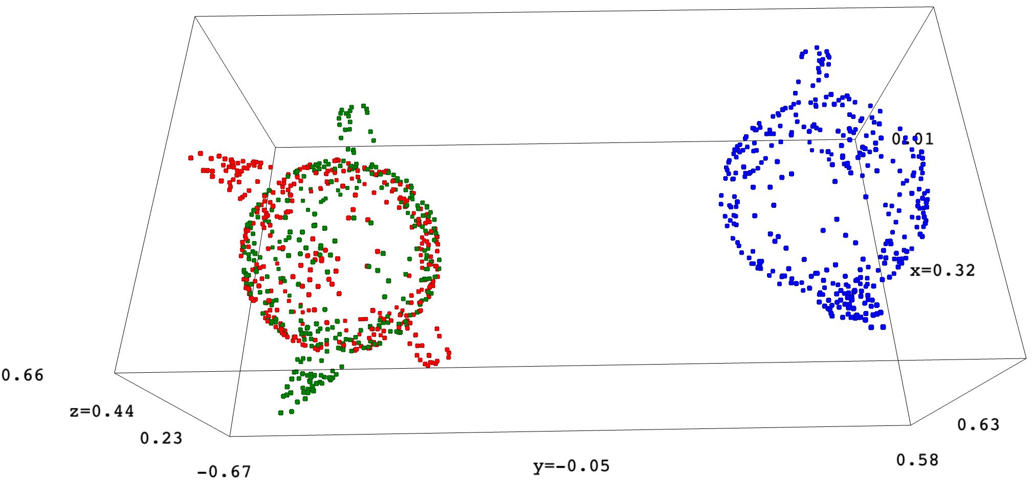
Figure 1: A typical result of ICP applied to the “teapot” cloud without initialization: the specimen cloud $P$ (blue), the image $Q$ (red) of $P$ under an orthogonal transformation, and the image of $P$ recovered by ICP (green).

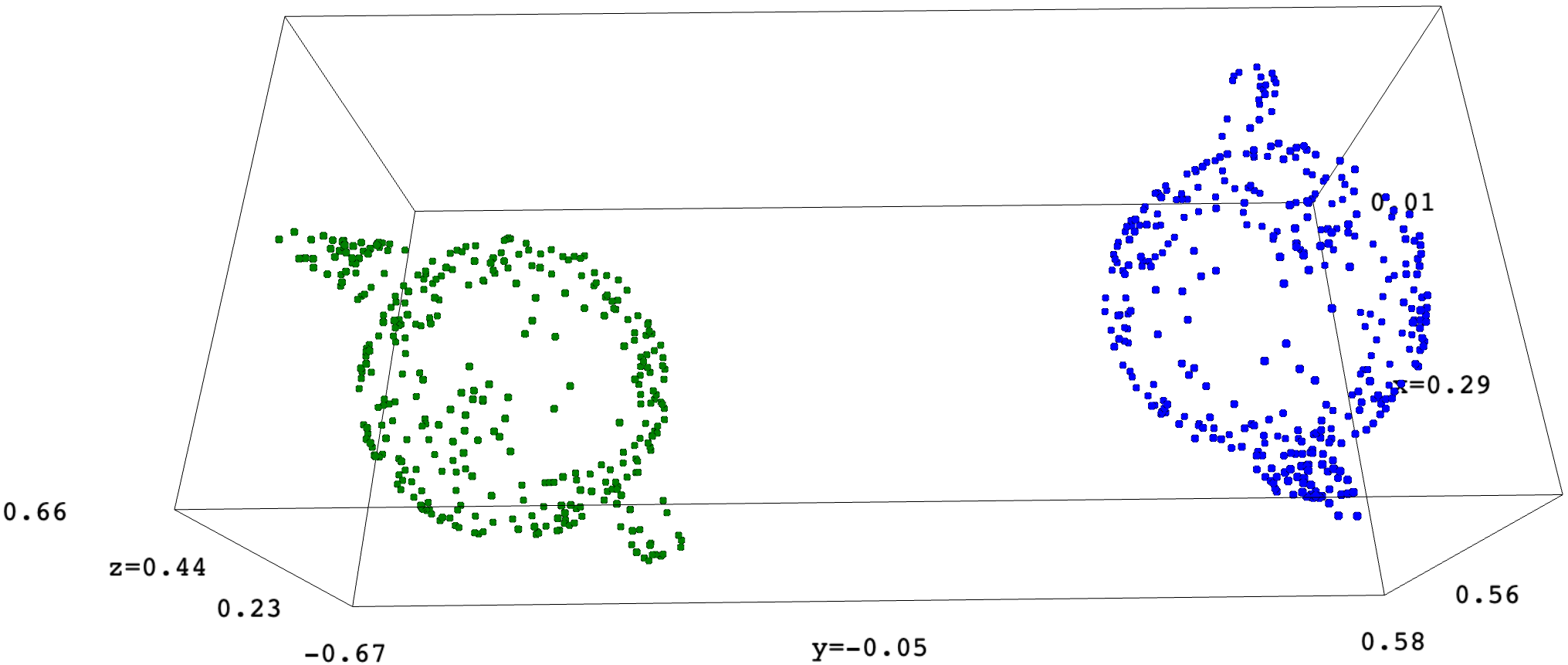
Figure 2: A typical result ICP applied to the “teapot” cloud with E–Init. The specimen cloud $P$ is in blue, while the image $Q$ of $P$ under an orthogonal transformation is red, and the image of $P$ recovered by ICP is green. The green and red images completely overlap.

VIII-E Multiplicative noise

$100$ tests were performed on each of the three unoccluded Caerbannog clouds [14]: the teapot, the bunny, and the cow. All tests were successful in recovering $O$ with relatively minor errors given that the noise is also relatively minor. Recovering the permutation $S$ fails in most cases as even relatively minor noise interferes seriously with the nearest neighbors matching.

In each test, we obtain an orthogonal transformation $U_{init}$ from our initialization algorithm and then an improved transformation $U_{icp}$ after running ICP. We also obtain the image of $P$ from ICP, i.e. $Q_{icp}=U_{icp}\,P\,S_{icp}$ and compare it to $Q^{\prime}$ after matching the nearest neighbors of $Q_{icp}$ and $Q^{\prime}$ using a matching matrix $S_{icp}$. We also compare $Q_{icp}$ to the actual specimen image $Q=O\,P\,S$ of $P$.

We find it instructive to compute the improvement that ICP makes to the initializing orthogonal transformation $U$, as well as the distance between $Q_{init}=U\,P\,S_{icp}$ and $Q_{icp}$.

In the tests, we used Gaussian (multiplicative) noise $\mathcal{N}(1,\sigma^{2})$ with $\sigma\in\{0.1,0.2,\cdots,0.6\}$.

In Fig. 5 we plot the success rate depending on the added noise $\nu$.

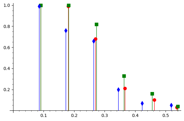
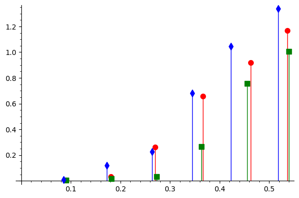
Figure 3: Success rate (vertical axis-$\tau$) depending on the multiplicative noise (horizontal axis-$\nu$) over $100$ tests for the “teapot” (red circle), “bunny” (green square), and “cow” (blue lozenge) point clouds. The experiments were carried out for Gaussian multiplicative noise $\mathcal{N}(1,\sigma^{2})$, $\sigma\in(0.1,0.2,\ldots,0.6)$.

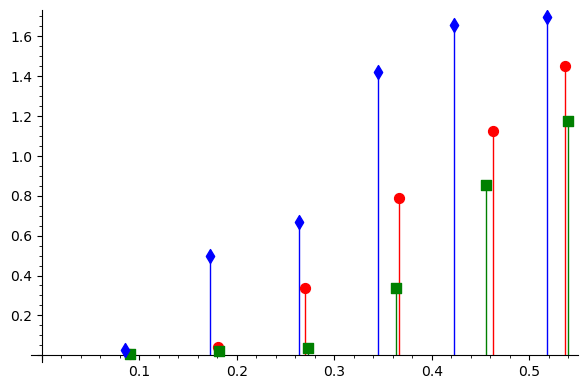
Figure 4: Normalized distance to the specimen depending on the multiplicative noise measured over $100$ tests for the “teapot” (red circle), “bunny” (green square), and “cow” (blue lozenge) point clouds. $\nu$ and $\delta_{spec}$ are computed for Gaussian multiplicative noise $\mathcal{N}(1,\sigma^{2})$, $\sigma\in(0.1,0.2,\ldots,0.6)$.

Figure 5: Distance to the original orthogonal transformation depending on the multiplicative noise measured over $100$ tests for each of the “teapot” (red circle), “bunny” (green square) and “cow” (blue lozenge) point clouds. The experiments were carried out for Gaussian multiplicative noise $\mathcal{N}(1,\sigma^{2}),\sigma\in(0.1,0.2,\ldots,0.6$).

Judging from Fig. 5, most tests fail for $\nu\leq 0.35$ (which approximately corresponds to $\sigma\geq 0.4$).

We also produce the plots for $\delta_{spec}$ (Fig. 5) and $\delta_{o}$ (Fig. 5) depending on $\nu$. In Fig. 6 the case of a noisy “teapot” cloud is shown.

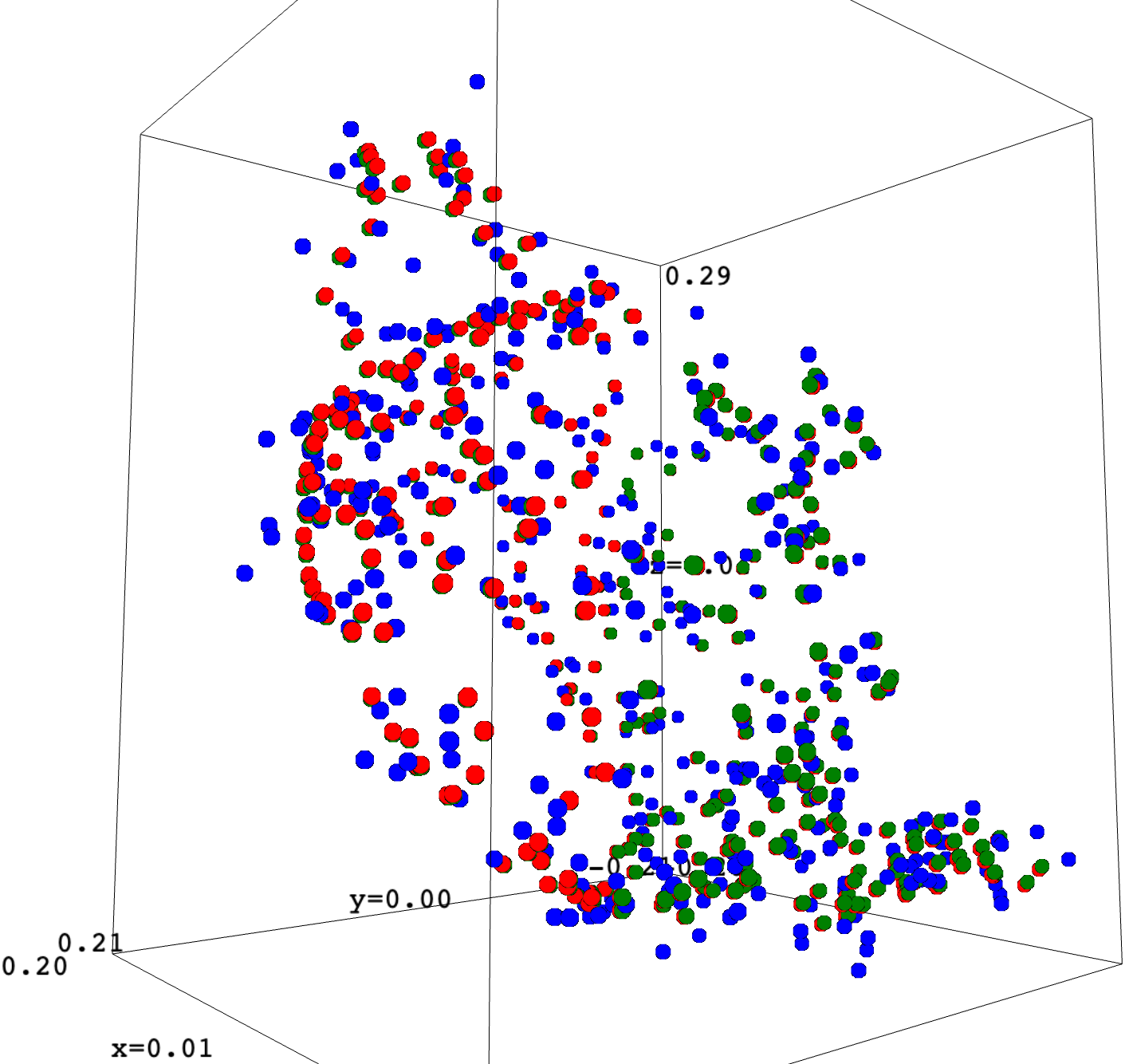
Figure 6: Multiplicative noise with $\nu=0.087$ ($\sigma=0.1$) on the “teapot” cloud. Shown in the plot is the specimen cloud $Q$ (red), the noisy cloud $Q^{\prime}$ (blue), and the recovered cloud $Q_{icp}$ (green). There is a significant overlap between the point clouds.

VIII-F Additive noise

$100$ tests as described above were performed on each of the three unoccluded Caerbannog clouds [14]: the teapot, the bunny, and the cow. The procedure and measurements were similar to the case of multiplicative noise.

In Fig. 7 we plot the success rates measured for different levels of noise by running $100$ tests in each case, for each of the Caerbannog clouds.

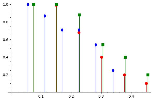
Figure 7: Success rate depending on the normalized additive noise measured over $100$ tests for each of the “teapot” (red circle), “bunny” (green square) and “cow” (blue lozenge) point clouds. $\nu$ and $\tau$ are computed for Gaussian multiplicative noise $\mathcal{N}(0,\sigma^{2})$, $\sigma\in(0.01,0.02,\ldots,0.06$),

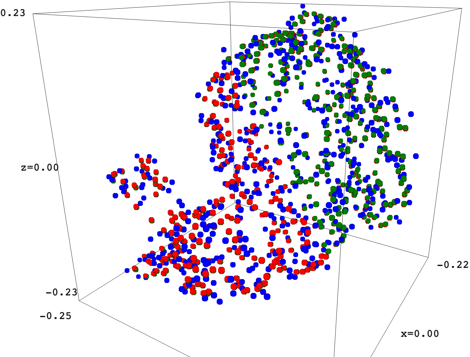
Figure 8: Additive noise with $\nu=0.074$ ($\sigma=0.01$) on the “bunny” cloud. Shown in the plot is the specimen cloud $Q$ (red), the noisy cloud $Q^{\prime}$ (blue), and the recovered cloud $Q_{icp}$ (green). There is a significant overlap between the point clouds.

In Fig. 8 the case of a noisy “bunny” cloud is shown.

Additional plots and test statistics are available in the GitHub repository [15].

VIII-G Occluded images

$100$ tests as described above were performed on each of the three unoccluded Caerbannog clouds [14]: the teapot, the bunny, and the cow. We used $P^{\prime}=P$ unoccluded as a specimen cloud, and $Q^{\prime}=Q\cup\Delta Q$ as its occluded image. Here $Q=O\,P\,S$, as described in Section V, and $\Delta Q$ was created as follows. First, we determine the rectangular bounding box $B$ for $Q$ with sides parallel to the coordinate planes and then generate uniformly inside $B$ random points $\Delta Q$. The cardinality of $\Delta Q$ is controlled by the level of occlusion $\alpha$: namely $|\Delta Q|$ is the integer part of $\alpha\,|Q|$.

In our tests, we used $\alpha\in\{0.2,0.4,\cdots,1.2\}$.

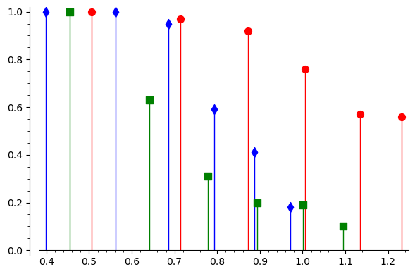
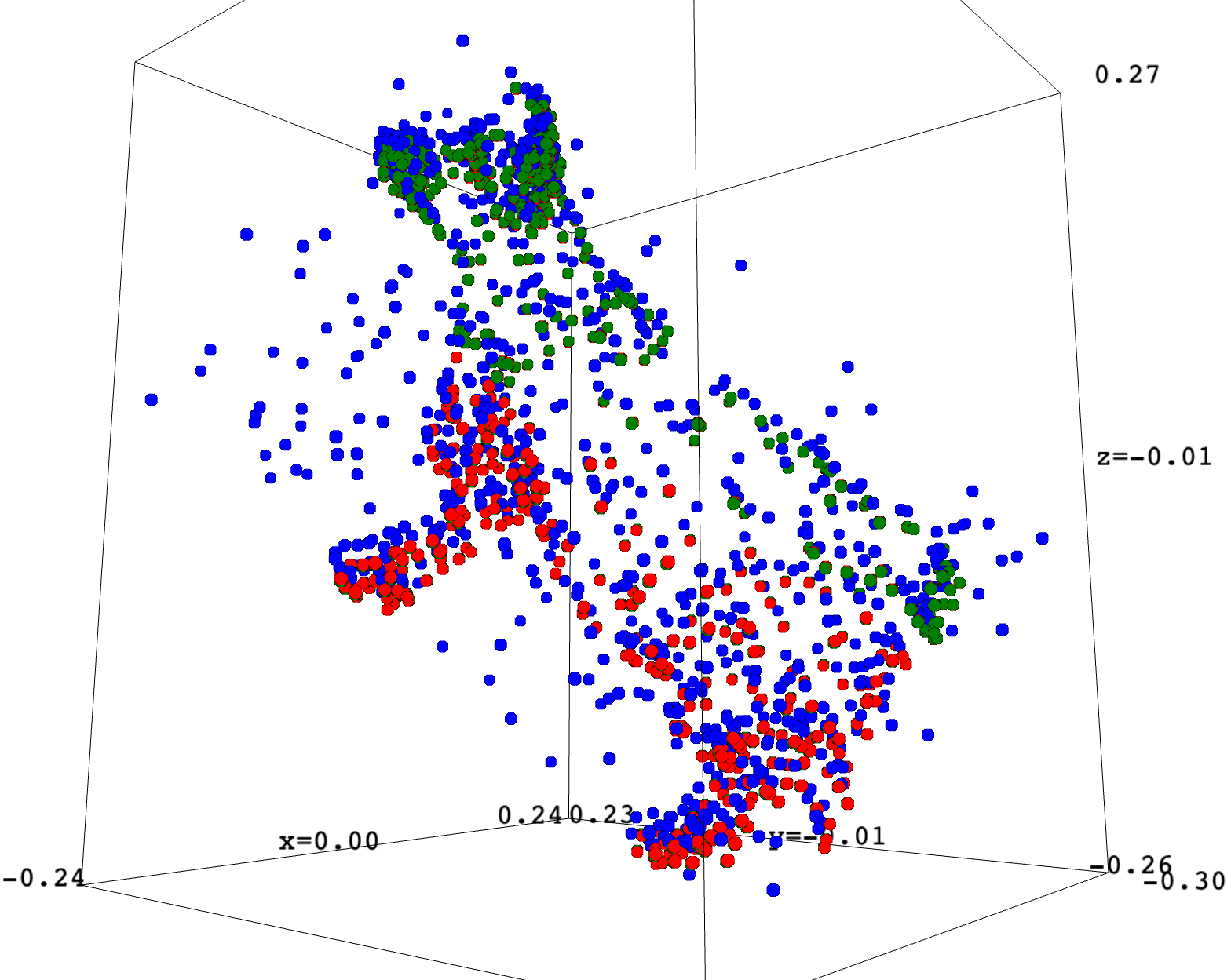
Figure 9: Success rate depending on the normalized occlusion averaged over $100$ tests for each of the “teapot” (red circle), “bunny” (green square) and “cow” (blue lozenge) point clouds. $\nu$ and $\tau$ are computed for occlusion levels $\alpha\in(0.2,0.4,\ldots,1.2)$.

Figure 10: Occlusion with $\nu=0.57$ ($\alpha=0.4$) on the “cow” cloud. Shown is the specimen cloud $Q$ (red), the occluded cloud $Q^{\prime}$ (blue), and the recovered cloud $Q_{icp}$ (green). There is a significant overlap between the point clouds.

In Fig. 10 we plot the success rates measured for different levels of noise by running $100$ tests in each case, for each of the Caerbannog clouds.

In Fig. 10 the case of a noisy “cow” cloud is shown. Additional plots are available in the GitHub repository [15].

VIII-H Superposition of errors

We provide the results of $100$ tests performed for various levels of occlusion, additive, and multiplicative noises superimposed on each of the Caerbannog clouds. For example, in Figures 12 – 12 the case of the “teapot” cloud is presented. In each figure, the level of occlusion is fixed, while we provide the dependence of the measured parameters on the values of $\sigma$ for additive and multiplicative noises. Additional plots are available on GitHub [15].

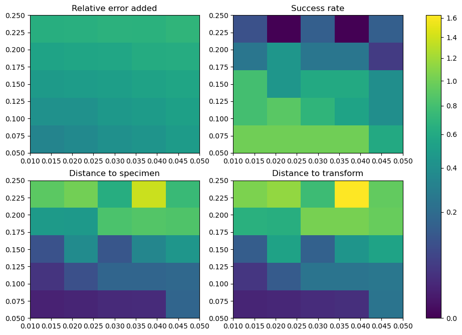
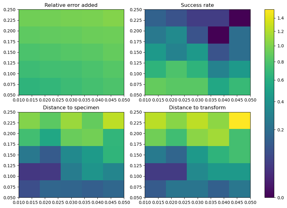
Figure 11: Colormap for the statistics of tests on the “teapot” point cloud matching $P$ to the occluded $Q^{\prime}$ with additive and multiplicative noises superimposed. Occlusion is formed by adding uniformly distributed points in the point cloud $Q$ bounding box: occlusion points are $5\%$ of the original cloud cardinality. The noise parameters: $\sigma$ for $\mathcal{N}(0,\sigma)$ additive noise is indicated on the horizontal axis, $\sigma$ for $\mathcal{N}(1,\sigma)$ multiplicative noise is indicated on the vertical axis.

Figure 12: Colormap for the statistics of tests on the “teapot” point cloud matching $P$ to the occluded $Q^{\prime}$ with additive and multiplicative noises superimposed. Occlusion is formed by adding uniformly distributed points in the point cloud $Q$ bounding box: occlusion points are $25\%$ of the original cloud cardinality. The noise parameters: $\sigma$ for $\mathcal{N}(0,\sigma)$ additive noise is indicated on the horizontal axis, $\sigma$ for $\mathcal{N}(1,\sigma)$ multiplicative noise is indicated on the vertical axis.

VIII-I Registering multiple scans

We compare two scanned images of the same sculpture before and after restoration in several cases shown in Figures 13, 15, 17 (see Section X, also for Figures 14, 16, 18).

Our E–Init algorithm performs well in this case, as shown in Figures 14 (right), 16 (right), 18 (right), used in conjunction with the out–of–the–box ICP supplied in open3d [16]. The latter applied without E–Init fails to register properly, as shown in Figures 14 (left), 16 (left), 18 (left). We used the point–to–plane version of ICP in all instances.

The ground truth for matching the broken and restored sculptures is shown in Figures 13 (center), 15 (center), 17 (center). It is worth mentioning that the statue has relatively light damages only in Figure 13, while in Figure 15 the broken and restored statues differ significantly. Also, in Figure 17 the ground truth alignment shows that the broken and restored images do not fully match.

The code and mesh data used are available on GitHub [15].

VIII-J Comparison to other algorithms

We use GO–ICP [7] as a state–of–the–art reference algorithm as it provides provably convergent branch–and–bound strategy for global search over the orthogonal group $\mathrm{O}(3)$. In our experiments, $10$ tests were performed on each of the Caerbannog point clouds [14] for comparison. With multiplicative noise $\mathcal{N}(1,\sigma)$ having $\sigma=0.1$

It is worth mentioning that normal multiplicative noise with $\sigma=0.1$ (in which case $0.08\leq\nu\leq 0.093$) requires the MSE parameter of GO–ICP to be set to $0.0001$. Lower values of the MSE parameter (e.g. $0.001$) result in the branch–and–bound method choosing the wrong branch at times. The time needed to find the right parameters, which are necessary to run GO–ICP, were not taken into consideration. The results showing a much larger computation time for GO–ICP than E–init are presented in Table I.

Model	Average time(s)	$\delta_{spec}$	$\delta_{o}$
Teapot GO–ICP	75.90	0.008	0.009
Teapot E–init	2.77	0.006	0.007
Bunny GO–ICP	103.64	0.011	0.012
Bunny E–init	6.35	0.004	0.005
Cow GO–ICP	18.17	0.011	0.012
Cow E–init	8.34	0.005	0.006

TABLE I: Comparison of E–init with GO–ICP.

VIII-K GitHub repository

The SageMath code used to perform the numerical experiments is available on GitHub at https://github.com/sashakolpakov/icp–init. The open source computer algebra system SageMath (freely available at https://www.sagemath.org/) is required to run the code.

IX Conclusion

This note presents an approach to initialize the Iterative Closest Point (ICP) algorithm to match unlabelled point clouds related by rigid transformations so that it finds good solutions. The method is especially pertinent when there is a large overlap between the centered point clouds and is based on matching the ellipsoids defined by the points’ covariance matrices and then trying the various principal half–axes matchings that differ by elements of the finite reflection group of the ellipse’s axial planes. We derive bounds on the robustness of our approach to noise and experiments confirm our theoretical findings and the usefulness of our initialization.

Alexander Kolpakov Alexander Kolpakov received his Ph.D. degree from the University of Fribourg, Switzerland, in 2013. Currently, he is an Assistant Professor at the University of Neuchâtel. His research interests are in the domains of Riemannian geometry and group theory, and also applications of geometry to data science and image processing.

Michael Werman Michael Werman received his Ph.D. degree from The Hebrew University, in 1986, where he is currently a Professor of Computer Science. His current research interests include designing computer algorithms and mathematical tools for analyzing, understanding, and synthesizing pictures.

X Appendix

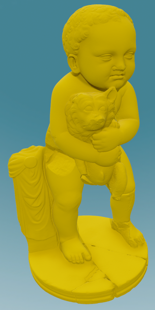
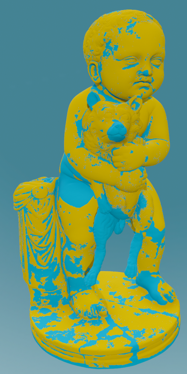
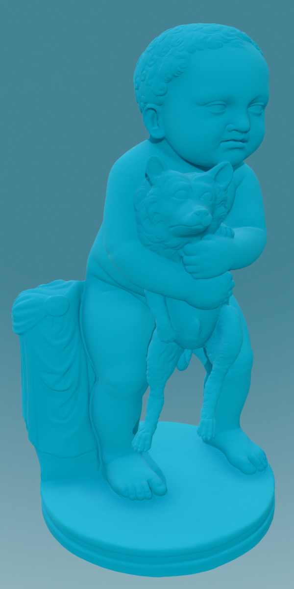
Figure 13: “Enfant au Chien” before (left) and after (right) restoration (available from [17]). The ground truth of matching the sculptures (center).

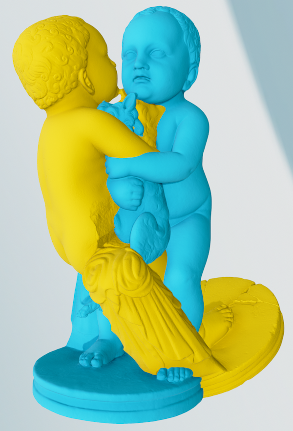
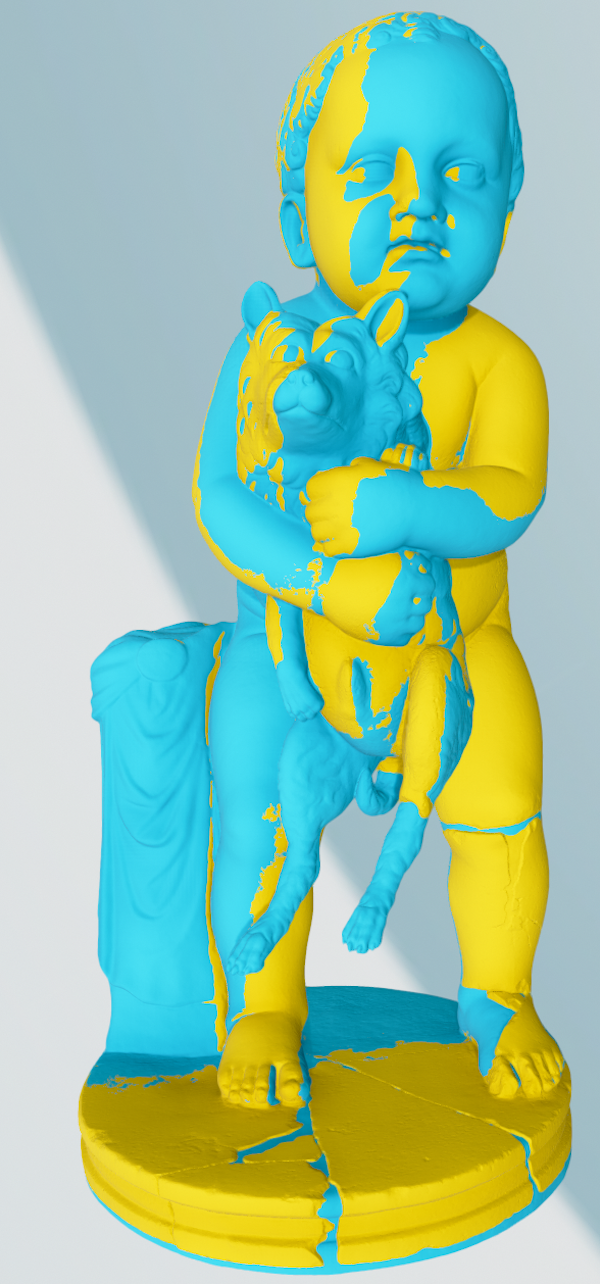
Figure 14: “Enfant au Chien” ICP registration: without initialization (left) and with initialization (right).

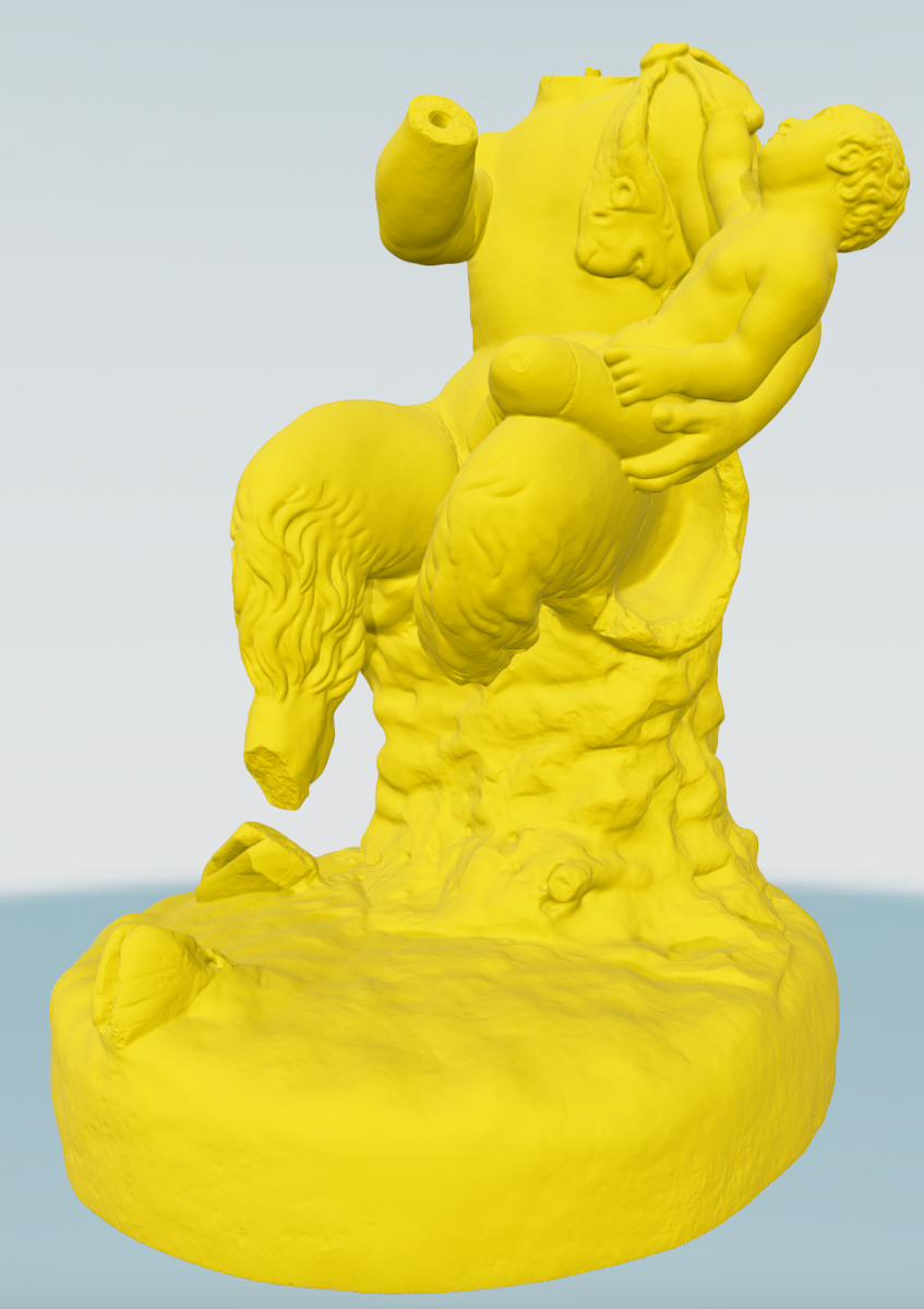
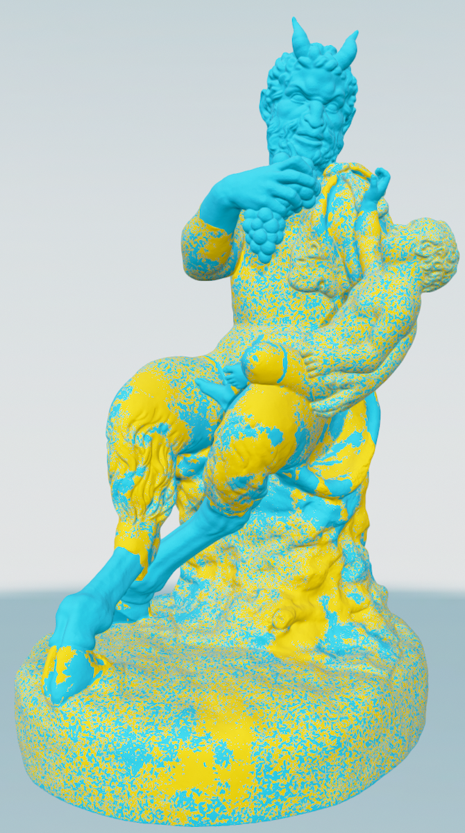
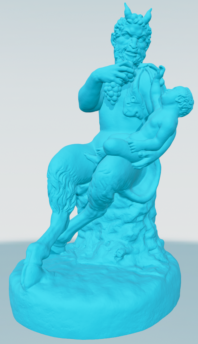
Figure 15: “Pan and Bacchus” before (left) and after (right) restoration (available from [17]). The ground truth of matching the sculptures (center).

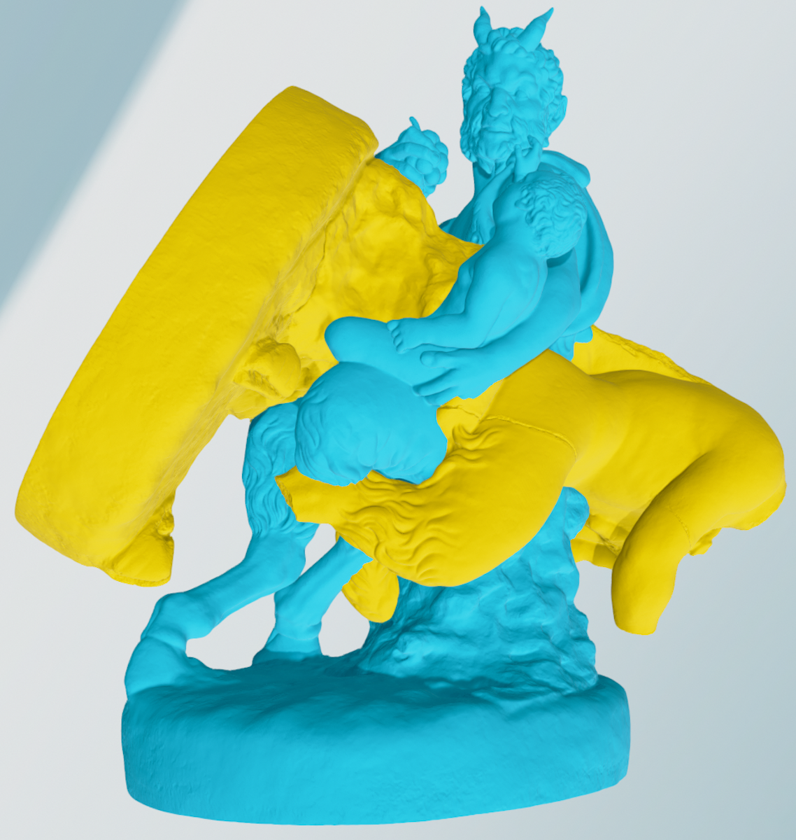
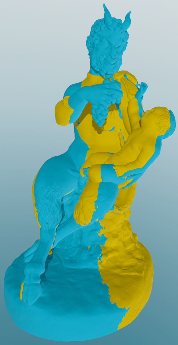
Figure 16: “Pan and Bacchus” ICP registration: without initialization (left) and with initialization (right).

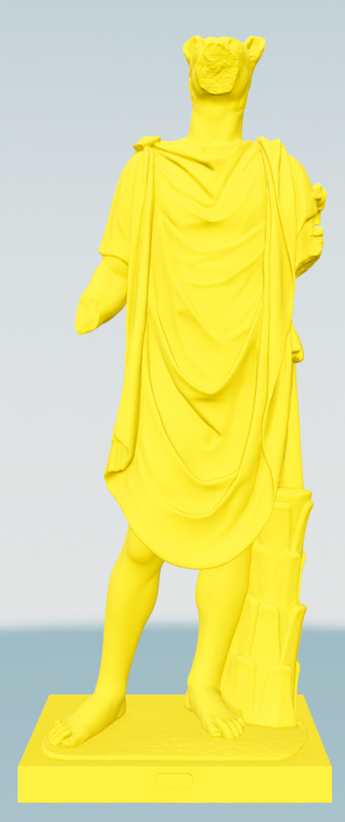
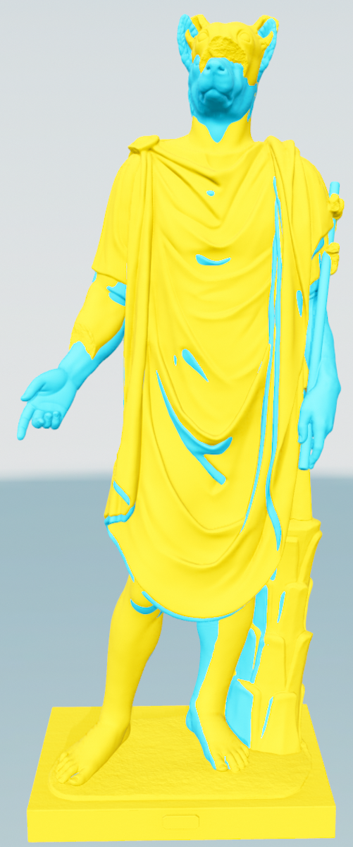
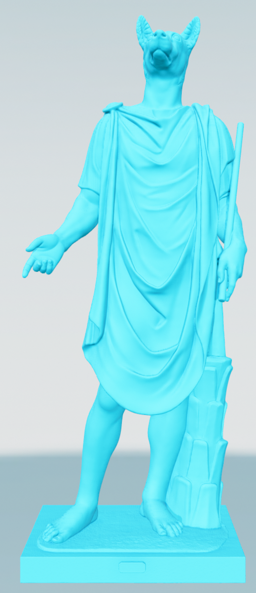
Figure 17: “Hermanibus” before (left) and after (right) restoration (available from [17]). The ground truth of matching the sculptures (center).

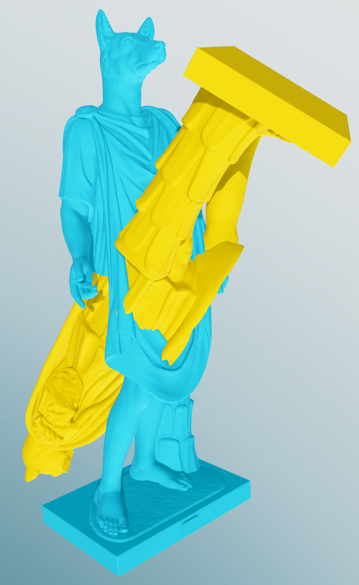
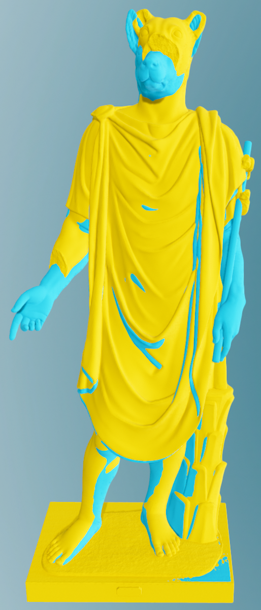
Figure 18: “Hermanibus” ICP registration: without initialization (left) and with initialization (right).

References

- [1] H. Si, J. Qiu, and Y. Li, “A review of point cloud registration algorithms for laser scanners: Applications in large–scale aircraft measurement,” Applied Sciences, vol. 12, no. 20, 2022. [Online]. Available: https://www.mdpi.com/2076-3417/12/20/10247
- [2] L. Li, R. Wang, and X. Zhang, “A tutorial review on point cloud registrations: Principle, classification, comparison, and technology challenges,” Mathematical Problems in Engineering, 2021.
- [3] P. Besl and N. D. McKay, “A method for registration of 3–D shapes,” IEEE Transactions on Pattern Analysis and Machine Intelligence, vol. 14, no. 2, pp. 239–256, 1992.
- [4] Y. Chen and G. Medioni, “Object modeling by registration of multiple range images,” in Proceedings. 1991 IEEE International Conference on Robotics and Automation, 1991, pp. 2724–2729 vol.3.
- [5] Wikipedia contributors, “Iterative closest point — Wikipedia, the free encyclopedia,” 2022. [Online]. Available: https://en.wikipedia.org/w/index.php?title=Iterative_closest_point&oldid=1095051621
- [6] W. Kabsch, “A solution for the best rotation to relate two sets of vectors,” Acta Crystallographica Section A, vol. 32, no. 5, pp. 922–923, 1976. [Online]. Available: https://doi.org/10.1107/S0567739476001873
- [7] J. Yang, H. Li, D. Campbell, and Y. Jia, “GO–ICP: A globally optimal solution to 3D ICP point–set registration,” IEEE transactions on pattern analysis and machine intelligence, vol. 38, no. 11, pp. 2241–2254, 2015.
- [8] X. Huang, G. Mei, J. Zhang, and R. Abbas, “A comprehensive survey on point cloud registration,” arXiv preprint arXiv:2103.02690, 2021.
- [9] J. Serafin and G. Grisetti, “Nicp: Dense normal based point cloud registration,” in 2015 IEEE/RSJ International Conference on Intelligent Robots and Systems (IROS). IEEE, 2015, pp. 742–749.
- [10] ——, “Using extended measurements and scene merging for efficient and robust point cloud registration,” Robotics and Autonomous Systems, vol. 92, pp. 91–106, 2017.
- [11] A. Makovetskii, S. Voronin, V. Kober, , and A. Voronin, “A regularized point cloud registration approach for orthogonal transformations,” Journal of Global Optimization, 2022.
- [12] V. Arnold, “Modes and quasimodes,” Func. Anal. Appl., vol. 6, no. 2, pp. 94–101, 1972.
- [13] R. Ahlswede and A. Winter, “Strong converse for identification via quantum channels,” IEEE Trans. Inf. Theory, vol. 48, no. 3, pp. 569–579, 2002, [Addendum ibid 49(1):346, 2003].
- [14] S. Raghupathi, N. Brunhart-Lupo, and K. Gruchalla, “Caerbannog point clouds. National Renewable Energy Laboratory,” 2020. [Online]. Available: https://data.nrel.gov/submissions/153
- [15] A. Kolpakov and M. Werman, “SageMath worksheets for ICP initialization,” 2022. [Online]. Available: https://github.com/sashakolpakov/icp-init
- [16] Q.-Y. Zhou, J. Park, and V. Koltun, “Open3D: A modern library for 3D data processing,” arXiv:1801.09847, 2018.
- [17] O. Laric, “Three D Scans,” 2012. [Online]. Available: https://threedscans.com/