Distinguishing quantum dynamics via Markovianity and Non-Markovianity

Abstract

To study various quantum dynamics, it is important to develop effective methods to detect and distinguish different quantum dynamics. A common non-demolition approach is to couple an auxiliary system (ancilla) to the target system, and to measure the ancilla only. By doing so, the target system becomes an environment for the ancilla. Thus, different quantum dynamics of target systems will correspond to different environment properties. Here, we analytically study XX spin chains presenting different kinds of quantum dynamics, namely localized, delocalized, and dephasing dynamics, and build connections between Markovianity and non-Markovianity — the two most common properties of an environment. For a qubit coupled to the XX chain, we derived the reduced density matrix of the qubit through the projection method. Furthermore, when dephasing noise was introduced to the XX chain, we generalized the projection method by introducing an open-system interaction picture — a modification of the Dirac interaction picture. By calculating the reduced density matrix for the qubit analytically and numerically, we found that the delocalized (localized) chain corresponds to the Markovian (non-Markovian) bath when boundary effects are not considered, and the feature of the chain with dephasing noise as a bath is dependent on the dephasing strength. The three kinds of quantum dynamics can be distinguished by measuring the qubit only.

I introduction

Different quantum systems will present different types of quantum dynamics. In closed quantum system, the localization and thermalization (or delocalization) are two typical quantum dynamics. At long times, the thermalized system effectively reaches thermal equilibrium, even though as a whole it remains in a pure quantum state, but the localized system will keep the memory of initial state even at infinite time Hamacher et al. (2002); Abanin et al. (2019); Bañuls et al. (2017). The third dynamics, diffusion, is between the two types above. This can be realized in open systems, such as free fermion chain under continuous measurements or dephasing noiseLi et al. (2018); Medvedyeva et al. (2016a); Mendoza-Arenas et al. (2013). The dephasing system will eventually become maximal mixed states, and will not keep the information of the initial state at infinite time, but the evolution is much slower than the thermalization or delocalization.

Distinguishing different quantum dynamics in experiment is an important task. Some methods have been proposed to distinguish different dynamics. For example, by measuring the out-of-time-order correlation (otoc) in the quantum system, one can quantify the scrambling of quantum information in system, and therefore the otoc can distinguish the dynamics of quantum phase by measuring the systemKukuljan et al. (2017); Campisi and Goold (2017); Shen et al. (2017). However, the probe is difficult and requires too much resources.

Another way to probe the dynamics of quantum system is to use ancillary systems, such as a qubit attached to a quantum chain. Such hybrid systems have been studied before, where the decoherence and the quantum revival of the qubit have different characteristic for localized and delocalized quantum chainvan Nieuwenburg et al. (2016); Vasseur et al. (2015); Apollaro et al. (2011); Eleuch et al. (2017). It is interesting to treat this problem with open quantum system theory. For the ancillary qubit, the chain is environment, and the dynamics of quantum systems is connected with the feature of environment. In open quantum system, there are two types of environment, Markovian and non-MarkovianLindblad (1979); Laine et al. (2010); Breuer et al. (2016). An environment is said to be Markovian if it continuously loses the memory of the open system. On the contrary, for a non-Markovian environment, it stores the memory of the open system.

In this work, we study a qubit coupling to a quantum spin XX chain, and the chain can be exposed to dephasing noise, as illustrated in Fig.1. We connect the properties of environment to the dynamics of chain, and then distinguish the dynamics of the quantum system through investigating the evolution of the qubit. We consider the three kinds of dynamics mentioned. Since different dynamics may correspond to different properties of the bath, we calculate the reduced density matrix of the qubit and obtain the non-Markovianity of the bath from it. For the closed chain, we use the method of projection operator methodBreuer and Petruccione (2002) to get an explicit expression of the master equation for the qubit. Introducing dephasing noise to the quantum chain, we use the open quantum system theory to trace out the environment and derive the master equation for the qubit. Thus, we generalize the method to solving the evolution of the qubit coupling to a dephasing chain.

Our results shows that we can distinguish these three kinds of quantum dynamics by measuring the ancillary qubit. Especially, we measure the particle in qubit, which is equal to the probability the qubit is in spin up. In the first case, the dynamic is delocalization. The information will flow to the chain and then bounce back from the right boundary, and the bounce is a non-Markovian effect. In the second case, because we add dephasing noise to the chain, the bounce will decay and vanish when dephasing strength $\gamma$ is larger than a critical value $\gamma_{c}$, and we predict the critical dephasing strength $\gamma_{c}$ is inversely proportional to $N+1$. When $\gamma$ is strong, the transport in the chain becomes diffusive and is suppressed following $1/\gamma$, but the particle in qubit will decay slowly until the total system reaches the maximal mixed states, where the bath is Markovian. In the third case, when the XX chain is localized, the bath is strong non-Markovian, and the information can hardly flow to the chain.

The paper is organized as follows. In Sec.II, we introduce our model, we will first analytically studied the closed case without dephasing noise. Then we generalize the method to open system, derive the master equation of qubit’s reduced matrix, and obtained an explicit expression. In Sec.III, we show the analytical and exact diagonalization results for different cases, and use the analytical result to predict the critical dephasing strength $\gamma_{c}$, at which the bath transits from non-Markovian to Markovian. Furthermore, we calculate the transport in the chain with strong dephasing. In the end, we consider the localization case with strong disorder. In Sec.IV, we summarize our main results and make some discussion.

II Model and Method

Model. —— We consider a single qubit coupled to a N sites XX chain, as shown in Fig.1. The Hamiltonian of the total system is

$$H=H_{S}+H_{B}+H_{I}=H_{0}+H_{I},$$ (1)

where $H_{S}=\omega_{0}\sigma_{s}^{+}\sigma_{s}^{-}$ is the hamiltonian of the single qubit system, $H_{B}=J\sum_{i=1}^{N-1}(S_{i}^{x}S_{i+1}^{x}+S_{i}^{y}S_{i+1}^{y}+h_{i}S_{i}^{z})$ is the Hamiltonian of XX model with free ends, and $H_{I}=g(\sigma_{s}^{+}S_{1}^{-}+\sigma_{s}^{-}S_{1}^{+})$ describes the interaction between qubit and chain. We consider the initial states with qubit spin up and all spins in XX chain are spin down, $|\phi(t_{0})\rangle_{S}=|1\rangle_{S}$, $|\psi(t_{0})\rangle_{B}=|\psi_{B}\rangle=|0\rangle_{1}|0\rangle_{2}...|0\rangle_{N}$, with $|1\rangle$ to label spin up and $|0\rangle$ spin down.

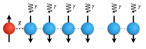
Figure 1: A single qubit coupling to a XX spin chain with coupling strength $g$, and the XX chain can be exposed to some dephasing noise, with the dephasing strength $\gamma$. When $\gamma=0$, the total system is a closed quantum system.

Closed case. —— We first calculate the case where the XX chain in the absence of dephasing, then the total system is a closed quantum system, the evolution of the total system is determined by Schrödinger equation. We want to trace out the bath and get the effective dynamical equation for qubit’s reduced density matrix, so as to know the flow of information between the qubit and the chain.

In the absence of dephasing, we would expect to see particle move right, then bounce from the right boundary and back to qubit. We use the projection operator methodBreuer and Petruccione (2002) to calculate the evolution of the reduced density matrix of the qubit.

When the total system is a closed quantum system, we can work in the interaction representation, and the equation of motion for the density matrix reads

$$\frac{\partial}{\partial t}\rho(t)=-ig\left[H_{I}(t),\rho(t)\right]\equiv g\mathcal{\mathcal{L}}(t)\rho(t),$$ (2)

where $H_{I}(t)=\exp(iH_{0}t)H_{I}\exp(-iH_{0}t)$ is the interaction Hamiltonian in interaction picture, and $\mathcal{L}(t)$ is the Liouville super-operator. In order to derive an exact equation of motion for the reduced density matrix $\rho_{s}$, we define a super-operator $\mathfrak{\mathcal{P}}$ according to $\mathfrak{\mathcal{P}}\rho(t)=tr_{B}\left[\rho(t)\right]\otimes\rho_{B}$, the $\rho_{B}$ can be an arbitrary density matrix in the bath, and here we choose $\rho_{B}=|\psi_{B}\rangle\langle\psi_{B}|$, and $\mathcal{Q}\rho(t_{0})=\rho(t_{0})-\mathfrak{\mathcal{P}}\rho(t_{0})$ is complementary super-operator. Then exact equation of motion of $\mathfrak{\mathcal{P}}\rho(t)$ can be written as

$$\frac{\partial}{\partial t}\mathfrak{\mathcal{P}}\rho(t)=\mathcal{K}(t)\mathfrak{\mathcal{P}}\rho(t)+\mathcal{I}(t)\mathcal{Q}\rho(t_{0}),$$ (3)

this is the exact time-convolutionless(TCL) form of the master equation, and $\mathcal{K}(t)=\sum_{n}g_{n}\mathcal{K}_{n}(t)=g\mathcal{P\mathcal{L}}(t)\left[1-\sum(t)\right]^{-1}\mathcal{P}$ is the TCL generator, $\sum(t)$ is super-operator $g\int_{t_{0}}^{t}ds\mathfrak{\mathcal{G}}(t,s)\mathcal{Q}\mathcal{L}(s)\mathfrak{\mathcal{P}}G(t,s)$. $\mathcal{I}(t)$ is the inhomogeneity, and we have $\mathcal{Q}\rho(t_{0})=0$ because the initial state is a product state, and then the second term on the right of the Eq.(3) is zero. So we can get the evolution of $\mathfrak{\mathcal{P}}\rho(t)$ by calculating $\mathcal{K}(t)$ in order.

The first order of $\mathcal{K}_{n}(t)$ is $\mathcal{K}_{1}(t)=\mathcal{PL}(t)\mathcal{P}$. For the interaction Hamiltonian we chosed, it satisfies $tr_{B}\{H_{I}(t)\rho_{B}\}$, which leads to the relation $\mathcal{K}_{1}(t)=0$. The lowest order non-zero $\mathcal{K}_{n}(t)$ is $\mathcal{K}_{2}(t)=\int_{0}^{t}dt_{1}\mathcal{PL}(t)\mathcal{L}(t_{1})\mathcal{P}$, and then we get the equation of motion for $\rho_{s}(t)$ up to second order:

$$\frac{\partial}{\partial t}\rho_{s}(t)=-g^{2}\int_{0}^{t}dt_{1}tr_{B}[H_{I}(t),[H_{I}(t_{1}),\rho_{s}(t)\otimes\rho_{B}]].$$ (4)

Using $H_{I}(t)=\exp(i\omega_{0}t)\sigma_{s}^{+}S_{1}^{-}(t)+\exp(-i\omega_{0}t)\sigma_{s}^{-}S_{1}^{+}(t)$ we can get:

$$\frac{\partial}{\partial t}\rho_{s}(t)=-g^{2}\int_{0}^{t}dt_{1}\times$$ (5)

$$\{e^{i\omega_{0}(t-t_{1})}tr_{B}[S_{1}^{-}(t)S_{1}^{+}(t_{1})\rho_{B}](\sigma^{+}\sigma^{-}\rho_{s}(t)-\sigma^{-}\rho_{s}(t)\sigma^{+})+$$

$$e^{-i\omega_{0}(t-t_{1})}tr_{B}[S_{1}^{-}(t_{1})S_{1}^{+}(t)\rho_{B}](\rho_{s}(t)\sigma^{+}\sigma^{-}-\sigma^{-}\rho_{s}(t)\sigma^{+})\}.$$

Consequently, we get the time derivative of the first diagonal element in qubit’s reduced density matrix:

$$\dot{\rho}_{s}^{11}(t)=-2g^{2}\mathfrak{Re}(tr_{B}[S_{1}^{-}(t)S_{1}^{+}(t_{1})\rho_{B}]e^{i\omega_{0}(t-t_{1})})\rho_{s}^{11}(t),$$ (6)

where $\mathfrak{Re}$ means the real parts. We can see that in the absence of dephasing, up to second order, the time derivative of particle number is determined by the time-dependent spin correlation $tr_{B}[S_{1}^{-}(t)S_{1}^{+}(t_{1})\rho_{B}]$ in XX chain.

This time-dependent spin correlation can be calculated by transforming XX model to the free fermion modelLieb et al. (1961); Mikeska and Pesch (12). After Jordan-Wigner transformation, $S_{i}^{+}=K(i)a_{i}^{\dagger}$ and $S_{i}^{-}=a_{i}K(i)$ with $K(i)=\exp[i\pi\sum_{i=1}^{N}(S_{j}^{z}+\frac{1}{2})]$, the Hamiltonian becomes $H=\frac{J}{2}\sum_{i=1}^{N-1}(a_{i}^{\dagger}a_{i+1}+a_{i}a_{i+1}^{\dagger})$, where ${{a_{i}}}$ and ${{a^{\dagger}_{i}}}$ satisfy anti-commutation relations of fermion operators. This Hamiltonian can be diagonalized to $H=J\sum_{k}\cos(k)a_{k}^{\dagger}a_{k}$, with $a_{k}=(\frac{2}{N+1})^{-\frac{1}{2}}\sum_{i=1}^{N}\sin(ki)a_{i}$, $k=\frac{m\pi}{N+1},m=1,2...N$. So $tr_{B}[S_{1}^{-}(t)S_{1}^{+}(t_{1})\rho_{B}]=\frac{2}{N+1}\sum_{k}\sin^{2}(k)e^{-i(t-t_{1})J\cos(k)}$. Then we get :

$$\dot{\rho}_{s}^{11}(t)=-\frac{4g^{2}}{N+1}(\sum_{k}\frac{\sin^{2}(k)\sin[(\epsilon_{k}+\omega_{0})t]}{(\epsilon_{k}+\omega_{0})})\rho_{s}^{11}(t),$$ (7)

where $\epsilon_{k}=J\cos(k)$. Back to the Schrödinger picture, the particle number in qubit is $n_{0}(t)=tr[e^{iH_{0}t}\hat{n}e^{-iH_{0}t}\rho_{s}(t)]=tr[\hat{n}e^{-iH_{0}t}\rho_{s}(t)e^{iH_{0}t}]=\rho_{s}^{11}(t)$, in which $\hat{n}=|1\rangle_{s}\langle 1|_{s}$. So Eq.(7) describes the time derivative of the particle number in qubit.

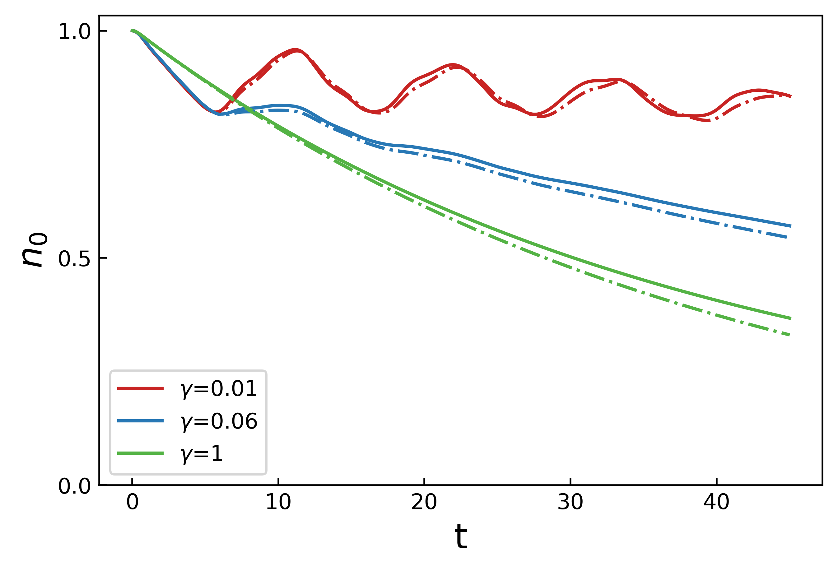
Figure 2: The particle number in qubit ($n_{0}$) as a function of time $t$. The solid line shows the result of exact diagonlization, and the dash line the result of TCL2. The plots are made by setting $g=0.2$, $J=4$, $\omega_{0}=0$, and $h_{i}=0$.

Dephasing case. —— When the XX chain is exposed to dephasing noise, the dynamics of the system is determined by the Lindblad master equation,

$$\frac{d\rho(t)}{dt}=-i[H,\rho(t)]+\gamma\sum_{i}(\sigma_{i}^{z}\rho(t)\sigma_{i}^{z}-\rho(t)).$$ (8)

We cannot transform to the traditional interaction picture and use an interaction Hamiltonian to generate the evolution. In order to solve the problem in perturbation, we introduce an open-system interaction picture, which is defined by $\tilde{\rho}(t)=e^{-(\mathcal{L}_{S}+\mathcal{L}_{B})t}(\rho(t))$, and then the evolution of $\tilde{\rho}(t)$ is determined by

$$\dot{\tilde{\rho}}(t)=\tilde{\mathcal{L}}(t)\tilde{\rho}(t)=e^{-(\mathcal{L}_{S}+\mathcal{L}_{B})t}\mathcal{L}_{I}e^{(\mathcal{L}_{S}+\mathcal{L}_{B})t}\tilde{\rho}(t),$$ (9)

where $\mathcal{L}_{S}\tilde{\rho}(t)=-i\left[H_{S},\tilde{\rho}(t)\right]$, $\mathcal{L}_{B}\tilde{\rho}(t)=-i\left[H_{B},\tilde{\rho}(t)\right]+\gamma\sum_{i}(\sigma_{i}^{z}\tilde{\rho}(t)\sigma_{i}^{z}-\tilde{\rho}(t))$, and $\mathcal{L}_{I}\tilde{\rho}(t)=-i\left[H_{I},\tilde{\rho}(t)\right]$. We also define super-operator $\mathfrak{\mathcal{P}}$ to project the density matrix, $\mathcal{P}\tilde{\rho}(t)=tr_{B}[\tilde{\rho}(t)]\otimes\rho_{B}$. Now the evolution of $\mathcal{P}\tilde{\rho}(t)$ can still be expressed as Eq.(3), and the only difference is that $\mathcal{L}(t)$ is changed to $\tilde{\mathcal{L}}(t)$, and $\rho(t)$ to $\tilde{\rho}(t)$.

The first order of $\mathcal{K}_{n}(t)$ can be expressed as $\mathcal{K}_{1}(t)=\mathcal{P}\tilde{\mathcal{L}}(t)\mathcal{P}$, and using $tr_{B}[\mathcal{L}_{B}(S_{1}^{+}\rho_{B})]=0$, we get $\mathcal{K}_{1}(t)=0$. So the lowest order non-zero $\mathcal{K}_{n}(t)$ is $\mathcal{K}_{2}(t)=\int_{0}^{t}dt_{1}\mathcal{P}\tilde{\mathcal{L}}(t)\tilde{\mathcal{L}}(t_{1})\mathcal{P}$, and then we get the equation of motion for $\tilde{\rho}_{s}(t)$ up to second order:

$$\frac{\partial}{\partial t}\rho_{s}(t) =-g^{2}\int_{0}^{t}dt_{1}\times$$ (10)

$$\{e^{i\omega_{0}(t-t_{1})}tr_{B}[S_{1}^{-}e^{\mathcal{L}_{B}(t-t_{1})}S_{1}^{+}\rho_{B}]\sigma^{+}\sigma^{-}\rho_{s}(t)-$$

$$e^{i\omega_{0}(t-t_{1})}tr_{B}[S_{1}^{-}e^{\mathcal{L}_{B}(t-t_{1})}S_{1}^{+}\rho_{B}]\sigma^{-}\rho_{s}(t)\sigma^{+}+$$

$$e^{i\omega_{0}(t_{1}-t)}tr_{B}[S_{1}^{+}e^{\mathcal{L}_{B}(t-t_{1})}\rho_{B}S_{1}^{-}]\rho_{s}(t)\sigma^{+}\sigma^{-}-$$

$$e^{i\omega_{0}(t_{1}-t)}tr_{B}[S_{1}^{+}e^{\mathcal{L}_{B}(t-t_{1})}\rho_{B}S_{1}^{-}]\sigma^{-}\rho_{s}(t)\sigma^{+}\}.$$

Using $\mathcal{L}_{B}(a_{k}^{\dagger}|\psi_{B}\rangle\langle\psi_{B}|)=(-i\epsilon_{k}-2\gamma)a_{k}^{\dagger}|\psi_{B}\rangle\langle\psi_{B}|$, we get the explicit expression for the time derivative of the first diagonal element $\dot{\tilde{\rho}}_{s}^{11}(t)$, which is equal to the time derivative of the particle numbers in qubit:

$$\dot{\tilde{\rho}}_{s}^{11}(t)=-\frac{4g^{2}\tilde{\rho}_{s}^{11}(t)}{N+1}({\sum_{k}}\sin^{2}(k)\times$$ (11)

$$\frac{e^{-2\gamma t}(-2\gamma\cos[(\epsilon_{k}+\omega_{0})t]+(\epsilon_{k}+\omega_{0})\sin[(\epsilon_{k}+\omega_{0})t])+2\gamma}{(\epsilon_{k}+\omega_{0})^{2}+4\gamma^{2}})$$

III Results

We have analytically obtained the particle number in qubit ($n_{0}$) by TCL2 method (second order time-convolutionless method). Furthermore, we can numerically calculate it by exact diagonalization method. In Fig. 2, we compare the results calculated with TCL2 and exact numeric solution for $N=10$. When the dephasing strength $\gamma$ is small, the particle in the qubit shows oscillation, and the oscillation will vanish when the dephasing strength $\gamma$ is greater than a critical value $\gamma_{c}$. It is shown that the TCL2 method and exact solution lead to almost the same results in the time duration in Fig. 2. It is clear that the TCL2 results catch the non-Markovianity for small $\gamma$ and Markovianity for large $\gamma$.

In our parameter range, the oscillation can be attributed to the boundary effect, correspond to the bounce from the right end of the chain and then back to the qubit, and the oscillation shows the non-Markovianity of bath (the chain and possible dephasing noise). It is worth noting that, for odd $N$ and $\omega_{0}=0$, the TCL2 results do not fit well with the exact numeric solution. Because the variable of cosine function in Eq. (5) and Eq. (11) is $\pi/2$, this term is 0 in denominator, which causes a non-negligible term, and makes perturbation theory fail. This can be solved by introducing a non-zero $\omega_{0}$.

In order to quantify the non-Markovianity, we define a bounce function $B(\Phi)=\int_{\dot{n}_{s}(t)>0}dt\dot{n}_{s}(t)$. It quantifies the bounce of the particle between the qubit and the chain. This is similar to the non-Markovianity defined in Breuer et al. (2009), but without taking over all pairs of initial states, our bounce function corresponds to one pair of initial states of the qubit: spin up and spin down.

In Fig. 3, we show the $\gamma$-depending bounce function for different $N$. For given $N$, $B(\Phi)$ decreases monotonously with $\gamma$ increasing, reaching zero at $\gamma=\gamma_{c}$. The $\gamma_{c}$ decreases with $N$ increasing. When $N$ is finite and $\gamma$ tends to zero, the $B(\Phi)$ is infinite. When $\gamma\neq 0$, the system always ends up reaching a steady state, and then $B(\Phi)$ is bounded.

In fact, we can derive $\gamma_{c}$ from Eq. (11). When $N$ is even and $\omega_{0}$ is zero, the mode of $k=\frac{N\pi}{2(N+1)}$ is dominant in the summation of k. We can roughly estimate $\gamma_{c}$ by solving the following inequality,

$$[e^{-2\gamma t}\sqrt{\epsilon_{k}^{2}+4\gamma^{2}}\sin(\epsilon_{k}t+\arctan(\frac{-2\gamma}{\epsilon_{k}}))+2\gamma]_{min}>0,$$ (12)

where the first term of the left side has a triangular function times a decaying exponential function. This indicates that the mode in the XX chain is exponentially suppressed by dephasing noise. This inequality holds for $\gamma>\gamma_{c}$. So we can get the critical dephasing strength $\gamma_{c}\simeq J\frac{ProducLog(\frac{3\pi}{2})}{3\pi}\sin\frac{\pi}{2(N+1)}\simeq\frac{0.862}{N+1}$. This matches the TCL2 results with all modes. These results are presented in Fig. 4.

In the case of strong dephasing noise, we calculate the particle transport in the chain. We have shown that the current $J_{i,i+1}=2(\sigma_{i}^{x}\sigma_{i+1}^{y}-\sigma_{i}^{y}\sigma_{i+1}^{x})$ is suppressed by the dephasing noise. In Fig. 5, we show $\log$$J_{i,i+1}^{max}$ as a function of $\gamma$. It is clear that the $\log$$J_{i,i+1}^{max}$–$\log(\gamma)$ plot is a straight line with slope -1 in the strong $\gamma$ regime, which indicates that the maximal value of the current in the strong dephasing noise is inversely proportional to $\gamma$. Furthermore, the light cone of the particle transport delays with $\gamma$ increasing, as shown in Fig. 6. This is similar to the $1/\gamma$ suppression in the diffusive coefficient of dephasing free fermion chainYang et al. (2022).

Now we use the second order perturbation theory to explain this phenomenon concisely. Similar to previous workCai and Barthel (2013); Medvedyeva et al. (2016b), we consider the dynamics of the chain under strong dephasing. The Liouvillian operator is divided into two parts, the non-perturbated terms and the perturbated term. The non-perturbated Louvilian is $\mathcal{L}_{0}(\rho(t))=\gamma\sum_{i}(\sigma_{i}^{z}\rho(t)\sigma_{i}^{z}-\rho(t))$, and the perturbation term is $\mathcal{L}_{1}(\rho(t))=-i[H_{xx},\rho(t)]$. Due to the strong dephasing, the non-diagonal terms in the density matrix decay rapidly, and then the density matrix tends to be diagonal, with $\rho_{0}^{\kappa}=\left|{\kappa}\right>\left<{\kappa}\right|$ satisfing $\sigma_{i}^{z}\left|{\kappa}\right>=\sigma_{i}\left|{\kappa}\right>$, and $\rho_{0}^{\kappa}$ is the stationary state of $\mathcal{L}_{0}$ . The action of $\mathcal{L}_{1}$ on the single diagonal matrix $\rho_{0}^{\kappa}$ results in $\mathcal{L}_{1}\rho_{0}^{\kappa}=-iJ\sum_{j}(|\kappa^{(j)}\rangle\left<{\kappa}\right|-\left|{\kappa}\right>\langle\kappa^{(j)}|)$, and $\langle\kappa|\kappa^{(j)}\rangle=0$, where $|\kappa^{(j)}\rangle=\frac{1}{2}(\sigma^{x}_{j}\sigma^{x}_{j+1}+\sigma^{y}_{j}\sigma^{y}_{j+1})|\kappa\rangle$. So the first order perturbation is zero, and the effective Liouvillian is $\mathcal{L}_{eff}=-P\mathcal{L}_{1}(1-P)\mathcal{L}_{0}^{-1}(1-P)\mathcal{L}_{1}P$ up to second order, where $P[\rho]=\sum_{\kappa}tr(\rho\rho_{0}^{\kappa})\rho_{0}^{\kappa}$. Then we get the effective Liouvillian in the subspace spanned by diagonal density matrix is

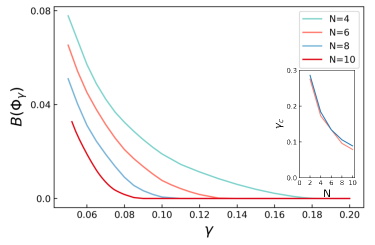
Figure 3: Bounce function $B(\Phi)$ as a function of $\gamma$ for $N=4,6,8,10$. Inset: $\gamma_{0}$ predicted by TCL2 and exact diagonalization, where the blue line shows the result of exact diagonalization, and the red line the result of TCL2.

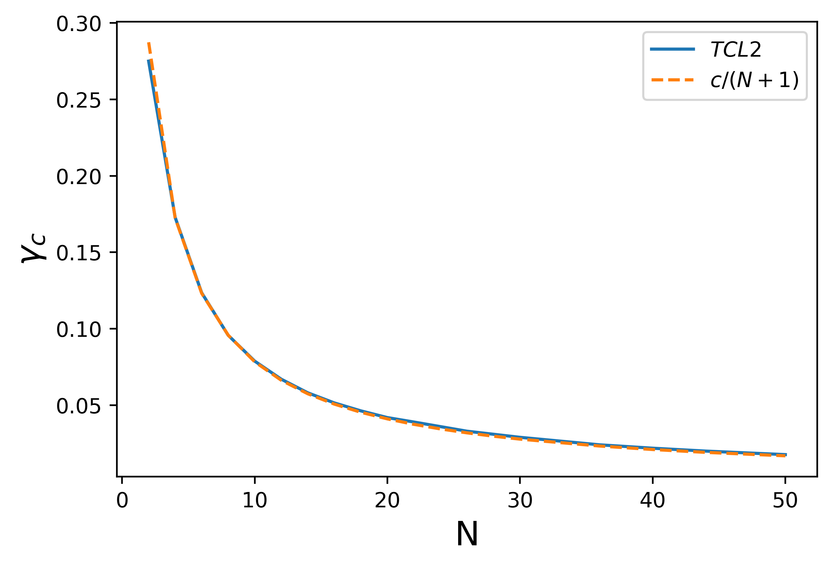
Figure 4: A comparison of the critical dephasing strength $\gamma_{c}$ in Eq.(11) as a function of $N$ (blue solid line) and the simple expression $c/(N+1)$ with $c=0.862$ (orange dashed line).

$$\mathcal{L}_{eff}\rho_{0}^{k}=\underset{j}{\sum}\underset{\kappa^{(j)}}{\sum}\langle\kappa^{(j)}|H_{eff}|\kappa\rangle|\kappa^{(j)}\rangle\langle\kappa|,$$ (13)

where $H_{eff}=\frac{J^{2}}{2\gamma}\underset{j}{\sum}(1-\vec{\sigma}_{j}\cdot\vec{\sigma}_{j+1})$, so the transport velocity is inversely proportional to $\gamma$.

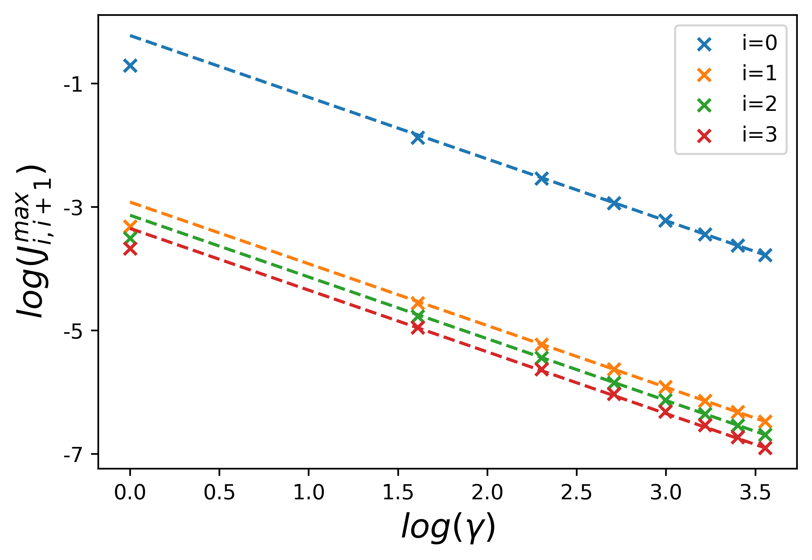
Figure 5: The maximum values of the current between site $i$ and site $i+1$, $J_{i,i+1}^{max}$ as a function of $\gamma$ for $i=0,1,2,3$. The slope of the double log plots is equal to $-1$.

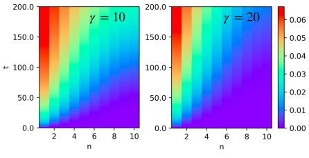
Figure 6: The particle number in the chain (with the scale shown on the right side) depending on lattice point $n$ and time $t$ for $\gamma=$10 and 20, with the parameters: $g=0.2$, $J=4$, $\omega_{0}=0$, and $h_{i}=0$.

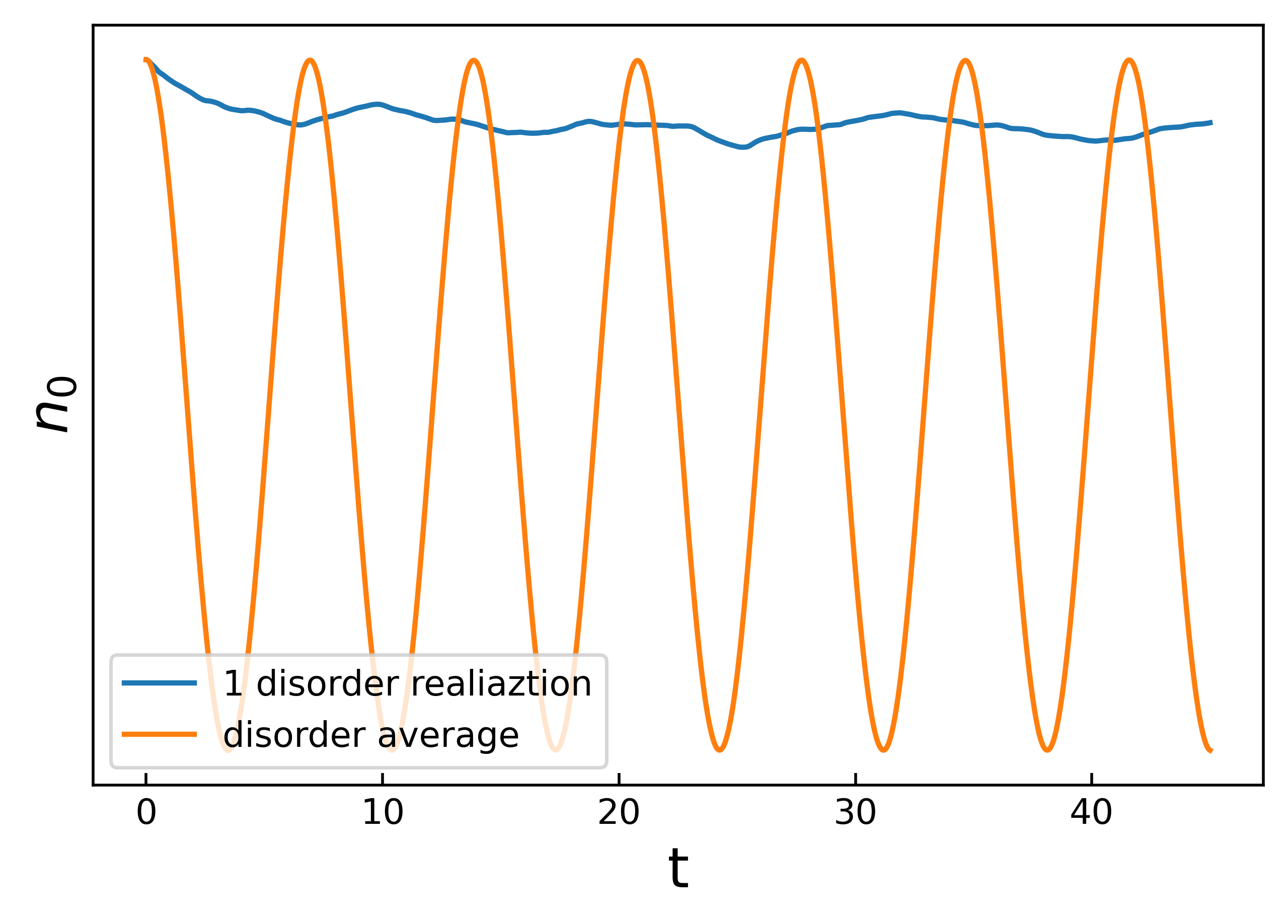
Figure 7: The time evolution of the particle number in qubit ($n_{0}$) for one disorder realization and that after disorder averaging, where $W=10$.

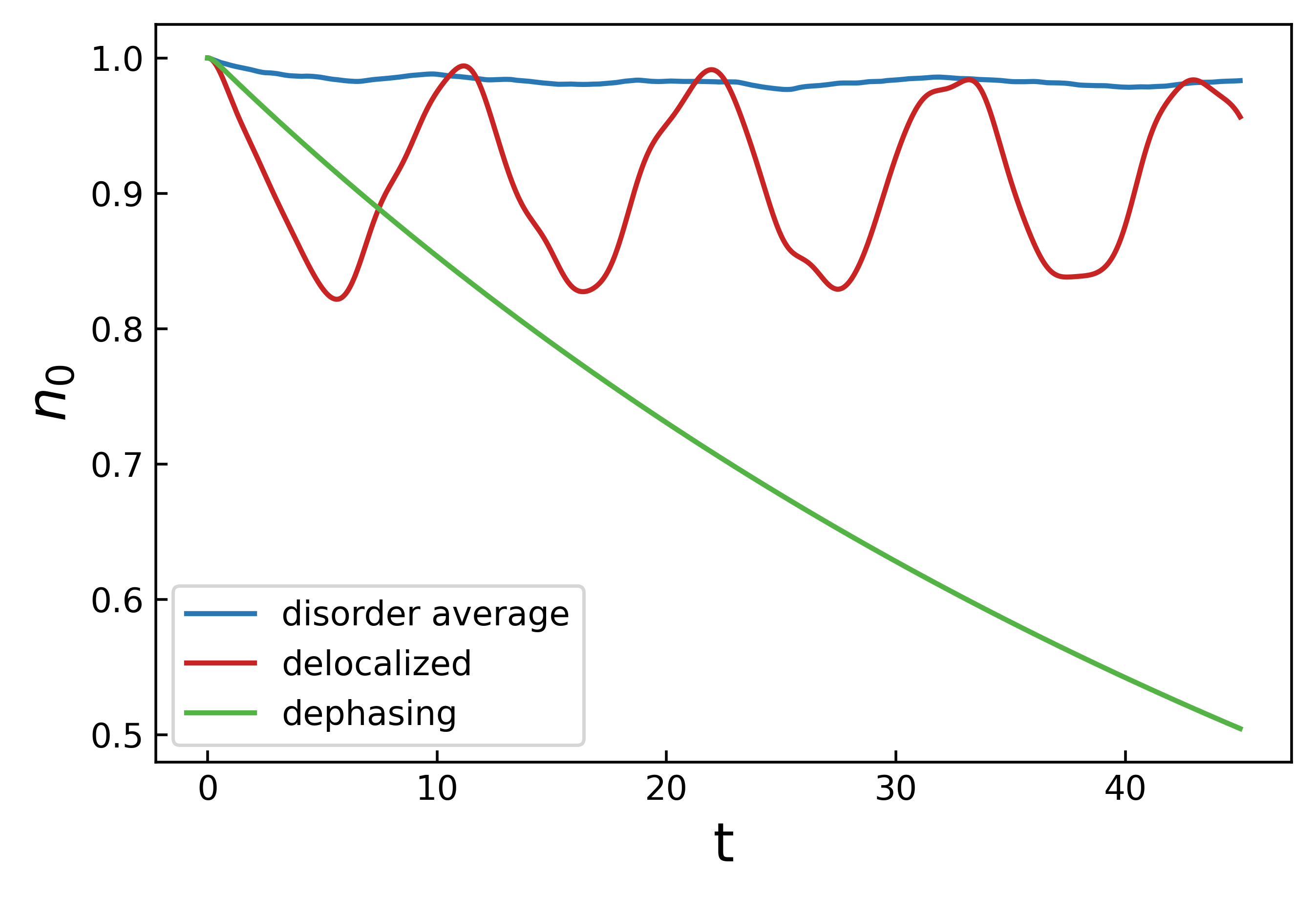
Figure 8: The particle number in qubit corresponding to the different cases for $N=10$, $g=0.2$, and $\omega_{0}=0$. $W=10$ and $\gamma=0$ for the localized case after disorder averaging, $W=0$ and $\gamma=0$ for the delocalized case, and $W=0$ and $\gamma=2$ for the dephasing case.

In the localization case, we set $\{h_{i}\}\in[-W,W]$, $W$ is the disorder strength, and the finite chain will be localizedAnderson (1958); Abou-Chacra et al. (1973) when $W$ is large. The evolution in one disorder realization is determined by Eq.(6), and the disorder average time derivative of particle should be

$$\dot{\rho}_{s}^{11}(t)=-2g^{2}\int_{0}^{t}dt_{1}\mathfrak{Re}(tr_{B}[\overline{S_{1}^{-}(t)S_{1}^{+}(t_{1})}\rho_{B}])\rho_{s}^{11}(t),$$ (14)

the over-bar means the disorder average. In each disorder realization, $tr_{B}[S_{1}^{-}(t)S_{1}^{+}(t_{1})\rho_{B}]$ should be oscillation term, and the frequency of oscillation is determined by $\{h_{i}\}$, so in each realization, the dynamics of qubit should be Markovian, as shown in Fig.7, the number of particle in qubit oscillates rapidlly. But after disorder average, this term tends to be zero, then the $\dot{\rho}_{s}^{11}(t)$ is almost zero.

The particle in qubit corresponding to different cases is shown in Fig.8. So we can distinguish the dynamics in the chain by measuring the qubit only. For these different dynamics, the bath correspond to Markovian or non-Markovian environment.

IV Discussion and Summary

When a qubit is coupled to the quantum XX chain, different XX chain dynamics corresponds to different bath properties, and we can distinguish these dynamics by measuring the ancillary qubit. The dynamics of the qubit will reflect the information of the bath. In the first case, for a finite chain in the absence of dephasing, the bath is non-Markovian due to the boundary effect, so the particle in the qubit will oscillate. For the second case, when the chain dynamics is localized, the bath is strong non-Markovian, the particle number in the qubit will oscillate rapidly. The non-Markovianity in the localized case is different from the first case because the revival in the localized case is much earlier than the bounce induced by the boundary effect, and the bounce of the delocalization case will vanish in the thermalization limit. For the third case, we introduce the dephasing noise. When the dephasing strength $\gamma$ increases, the bounce from boundary will decrease, which corresponds to the decay of non-Markovianity. For $\gamma>\gamma_{c}$, the bath is Markovian, and the particle of qubit will decrease and finally reaches a steady state.

In summary, using the projection operator method, we analytically derived the master equation for the qubit coupled to the XX chain. We consider three different kinds of dynamics in the XX chain: delocalization, localization, and diffusion. For the first two cases, since the total system is closed, we work in the traditional interaction picture and derive the master equation of the qubit’s reduced density matrix up to the second order. In the third case, considering the total system is an open system, we define the open system interaction picture and derive the master equation of the qubit’s reduced density matrix up to the second order, obtaining an explicit expression of the particle number in qubit. Our result shows that when the quantum system is delocalized, if the chain is finite length, the bath is non-Markovian due to the boundary effect, but no information flows back before the bounce from boundary, and the bounce function $B(\Phi)$ will be infinite. With the dephasing noise, $B(\Phi)$ will be bounded, and when $\gamma>\gamma_{c}$, $B(\Phi)=0$, and then the bath is Markovian. Our theoretical result shows that the $\gamma_{c}$ is inversely proportional to $N+1$. So in the delocalized case, the bath would be Markovian in the thermodynamic limit for any dephasing strength. We find that in the strong dephasing regime, the transport in chain is suppressed by $1/\gamma$, and we use a perturbation theory analysis to illustrate this phenomenon.