LoopDraw: a Loop-Based Autoregressive Model for Shape Synthesis and Editing

Abstract

There is no settled universal 3D representation for geometry with many alternatives such as point clouds, meshes, implicit functions, and voxels to name a few. In this work, we present a new, compelling alternative for representing shapes using a sequence of cross-sectional closed loops. The loops across all planes form an organizational hierarchy which we leverage for autoregressive shape synthesis and editing. Loops are a non-local description of the underlying shape, as simple loop manipulations (such as shifts) result in significant structural changes to the geometry. This is in contrast to manipulating local primitives such as points in a point cloud or a triangle in a triangle mesh. We further demonstrate that loops are intuitive and natural primitive for analyzing and editing shapes, both computationally and for users.

1 Introduction

Applying deep learning models on irregular data, particularly shapes and geometry (in contrast to regular data such as pixel grids in images), remains challenging. This is in part due to an underlying open question in geometry processing: how should shapes be represented? There is no settled universal representation among the many contenders, which include point clouds [25], meshes [11], voxels [29], and implicit functions [24], to name a few.

We present a new, compelling neural alternative for representing shapes using a loop primitive. A set of loops gives a sparse, yet informative portrayal of the underlying surface. We posit that loops have unique advantages compared to existing representations, allowing for intuitive user-editing, interpretable visual inspection, shape encoding, and better informed-reconstruction.

Representing 3D surfaces using planar cross-sectional slices has a long history in computer graphics, medical imaging, and geographical systems [2, 1, 17, 3, 33]. Each planar cross-section contains an arbitrary number of loops, and each loop is a closed two-dimensional contour. This work introduces LoopDraw, an autoregressive model for synthesizing 3D shapes based on cross-sectional loop sequences. The loops across all planes form an organizational hierarchy that we leverage for neural shape synthesis. The loop sequence data both describes the underlying surface, and prescribes a shape in the way it is reconstructed into a mesh.

We show that this loop representation, encoded as sequence data, presents an effective neural primitive for a generative model of 3D shapes via a transformer-based variational autoencoder (VAE): meshes are first sliced to yield loop data, which is then used to train an encoder and a decoder with a latent space bottleneck (see Fig. 3). The latent space smoothness offered by the VAE architecture and the intuitiveness and editability of loop data together form a powerful system for the controllable generation and refinement of 3D shapes. Tasks enabled by this framework include latent space sampling and interpolation between shapes, as well as manual loop editing during autoregressive decoding. This mid-decoding intervention allows meaningful, interpretable manipulation of the latent code by manual modification of loops (scaling, shifting, deformations); it also enables shape blending and completion by inserting loops transplanted from a different shape.

The autoregressive decoder produces a list of loops which can be manipulated on-the-fly, causing cascading effects on the remaining loops. This enables minimal edits to result in larger-scale effects to the resultant geometry (see Figs. 1, 7 and 4). This property illustrates how loops are a non-local description of the underlying shape. By contrast, editing other primitive representations tends to produce overly local effects, on the scale of individual triangles (in meshes), voxel cells (in voxel grids), or points (in point clouds). We may also contrast our approach with implicit neural representations which, while effective at reconstruction tasks, are not conducive to manual control post-generation [13].

Loops are an explicit representation of the underlying 3D surface. This enables accurately portraying sharp corners and high-frequency features of a surface (Figs. 1 and 5). Moreover, it is straightforward to obtain from closed planar loops the inside/outside information, necessary for surface reconstruction [22], in post-process. In contrast, point clouds require a consistent normal orientation for reconstruction, a notoriously difficult problem in geometry processing [22]. Lastly, loops are a native representation for 3D processing applications utilizing tomography (e.g. radio-imaging in biology and geology); our representation and system would offer a low-friction way to apply 3D generative modeling to these data domains [33, 7].

In summary, we present a loop primitive as a novel neural representation of 3D shapes. Loops accurately portray the underlying shape contours, and contain non-local surface information. Our architecture is designed to autoregressively encode and decode a hierarchical set of loops, using a transformer-based variational autoencoder. We also demonstrate that loops are intuitive and natural primitive for analyzing and editing shapes, both computationally and directly by human intervention.

[]

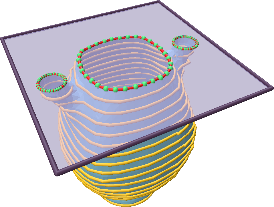
Figure 2: Closeup of a slice plane. In this example, the plane intersects the mesh at three closed loops, defining three time steps in our sequence data. Each loop has an associated level-up binary flag (shown as $\mathbf{0}$ or $\mathbf{1}$); the loop with a $\mathbf{1}$ flag introduces this slice plane and comes first in the sequence data, followed by the other loops with a flag of $\mathbf{0}$.

2 Related Work

Our approach joins a number of other works in the field of shape generation, specifically those that leverage sequences. Among autoregressive sequence-based generative frameworks, PolyGen [23] generates a sequence of mesh vertices and then learns to connect them together. Other works with diverse approaches to the sequence-based 3D shape modeling problem include DeepCAD [28]. We take inspiration from SketchRNN [10] and their neural representation of sketch strokes in the 2D vector graphics context. As far as we can ascertain, our work is the first technique to build a neural network for analyzing and synthesizing cross-sectional loops for shape generation and editing. This unique representation facilitates a method for achieving structural shape manipulations through simple and intuitive loop edits (such as geometric transformations) that imply broader changes to the resultant geometry.

Distinct from the autoregressive approach, several methods use implicit fields to model surfaces [6, 9, 24]. Such techniques achieve smooth intermediate shapes; yet, they may struggle to sharply represent discrete structural changes between shapes (often resulting in floating artifacts). The explicit mesh representation has been used for synthesizing fixed-topology modifications to shapes, such geometric texture synthesis [14] among others [20, 12]. As an alternative to generating shapes with fixed-topology, some techniques produce individual parts (e.g. meshes or cuboids) that are stitched together [30, 15]. Recently, TetGAN [8] proposed a hybrid representation of implicit and explicit methods in order to generate tetrahedral meshes with varying topology. Editing these primitive representations (such as loops, voxels, triangles, or volumetric cells) produce highly local effects. By contrast, loops are non-local, where simple geometric edits resulting in broad changes to the final shape. Our use of loops as a neural primitive takes inspiration from classic works that utilize cross-sectional planar slices [33, 31, 2]. Moreover, three dimensional loops (non-planar) are also related to quad-meshing and estimating sharp feature lines in 3D [4, 32].

[]

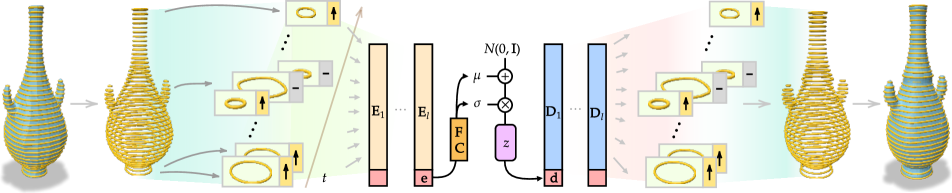
Figure 3: LoopDraw overview. Starting with an initial mesh, we extract a sequence of cross-sectional loops over a progression of planes. The entire sequence of loops (2D polygons with a level-up flag), augmented with a special token $\mathbf{e}$, is encoded through a series of $l$ transformer layers, producing features $[E_{1},\mathbf{e}_{1}],\dots,[E_{l},\mathbf{e}_{l}]$. The special token $\mathbf{e}_{l}$ in the last layer’s output is used as an aggregate encoder embedding that is then mapped to the parameters of a latent distribution. The latent vector $\mathbf{z}$ is projected to the start-of-sequence embedding $\mathbf{d}_{1}$ for the decoder, in which $l$ transformer layers produce $D_{1}\dots D_{l}$, which is trained to reconstruct the original input loop sequence. The reconstruction loss is the L2 distance (and cross-entropy for the binary flag) between the predicted and ground truth loop data, and a KL divergence term on the latent space parameters. The network-predicted loops are reconstructed to obtain a 3D mesh. In generation mode, we sample $\mathbf{z}$ from a standard Gaussian, and generate the sequence autoregressively.

3 Method

In this section, we describe the details of our framework (see illustration in Fig. 3). We define shapes using a sequence of closed cross-sectional loops (Sec. 3.1) and build a generative architecture for learning distributions of shapes using this representation (Sec. 3.2).

3.1 Loop Representation

Our loop-based representation of a 3D shape is defined by a sequence of planar cross-sectional contours. We slice along one axis of the shape, using an evenly spaced list of planes $P$. For each plane $p_{i}\in P$, we extract a set of loops $S$. The cross-sections with each slice plane $p_{i}$ are stored in $S$ as polylines, and we require all meshes used in this work to be manifold (in the areas that intersect the chosen slice planes); in other words, we enforce all loops in $S$ to be closed loops. After slicing, we resample the loops to contain $N$ (in our case $32$) vertices. Each closed loop is one time step (i.e., token) in the sequence $S$ along the slicing axis.

A plane is defined by a point $\mathbf{o}_{i}\in\mathbb{R}^{3}$ and a normal vector $\vec{n}_{i}\in\mathbb{R}^{3}$. Each plane $p_{i}$ in the list $P$ is encoded with these two vectors alongside two orthonormal vectors $\vec{x}_{i}$ and $\vec{y}_{i}$ which lie on the surface of the plane. Together these create a local coordinate system based on $p_{i}$ (with origin $\mathbf{o}_{i}$, $z$-axis $\vec{n}_{i}$, and $x-$ and $y-$ axes $\vec{x}_{i}$ and $\vec{y}_{i}$). Since our loops are planar (two-dimensional), each vertex of each loop on the plane $p_{i}$ can be represented with $\mathbb{R}^{2}$ coordinates with respect to this local system.

Even though each time step is one closed loop, each plane does not necessarily intersect the mesh at just one closed loop. We handle arbitrary number of per-plane loops by pairing each loop $s_{t}$ in $S$ (a closed polyline) with a binary level-up flag $u_{t}$.

This scheme implicitly records which plane each closed loop belongs to; the correspondence can be recovered by iterating across $S=([s_{1},u_{1}],\ldots,[s_{T},u_{T}])$ keeping track of the current plane $p_{i}$ in $P$ (initializing the state at $p_{0}$ which corresponds to no-plane): for each time step $t$, the loop described in $s_{t}$ is assigned to the current $p_{i}$ unless a level-up flag $u_{t}=1$, in which case we update $p_{i}:=p_{i+1}$ and assign the loop in $s_{t}$ to the new $p_{i}$. Thus, a slice plane having multiple cross-section polygons would accordingly be represented as multiple time steps in $S$, the first of which has a level-up flag set to $1$ and the rest having it set to $0$. See Fig. 2 for an illustration.

The per-loop polyline data is represented as a flattened vector of $N$ coordinates $s_{t}=\left[x_{1},y_{1},\dots,x_{N},y_{N}\right]$ with respect to the coordinate system on the plane $p_{i}$ to which the loop belongs. We impose a canonical ordering for this array of $N$ points such that $(x_{1},y_{1})$ is the loop point with minimum $(x+y)$, and the rest of the $(x,y)$ loop points will be arranged in clockwise order using their 2D coordinates on the plane coordinate system. Not all loops are convex, with a consistent clockwise orientation throughout, so this enforcement is heuristically based on the orientation of the first three points of a loop.

Reconstructing a mesh from loops

There exists methods to reconstruct meshes directly from contour loops [33]. Alternatively, because our loops are polylines and not unordered point sets, we may sample a point cloud and estimate surface normals directly from loops at arbitrary resolution (Fig. 6). This enables the option of reconstructing a mesh from an oriented point cloud sampled from loops.

3.2 Network Architecture

We model distributions of shapes represented as a sequence of loops using a variational autoencoder (VAE) [18]. This choice is motivated by the observation that an autoencoder design would allow for a smooth latent space of shapes. This complements the interpretability and ease of editing of the loop data itself, together enabling highly controllable, intuitive, and transparent generation and manipulation of loops and shapes. Our architecture leverages transformers [26] as the backbone for the encoder and decoder networks.

Encoder

The input to the encoder is a full loop data sequence of variable length, and the output is a fixed-size aggregate embedding that summarizes the shape based on this sequence. Specifically, the input is the sequence $S$ of loop parameters (as described in Sec. 3.1) plus a sinusoidal positional encoding.

To obtain this aggregate summary embedding, we insert a special token $\mathbf{e}$ (initialized to be $\mathbf{0}$) at the beginning of the input sequence. This is encoded through the transformer layers alongside the rest of the sequence. Then, we extract the output embedding from the final layer only at that first token slot $\mathbf{e}$ (corresponding to the special token appended to the input) (Fig. 3). This $\mathbf{e}$ is interpreted as an aggregate fixed-size embedding that describes the entire shape. The aggregate embedding is passed through MLPs to predict the parameters $(\mu,\log\sigma^{2})$ of a distribution in $N_{z}$-dimensional latent space. Using the reparameterization trick, we use these parameters to sample a latent code $\mathbf{z}$ for the decoder.

[]

[]

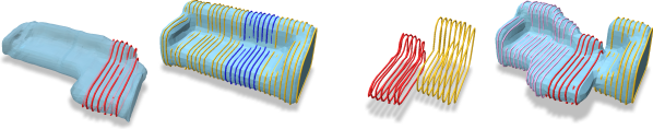
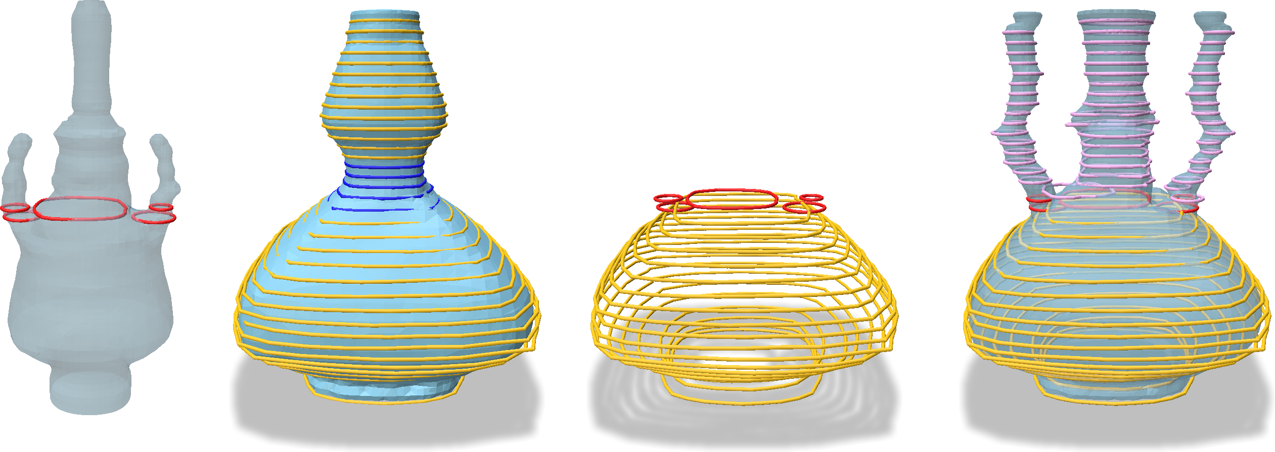
Figure 4: Loop transplantation. By taking new loops (e.g., handles) hand-drawn or extracted from a donor shape, manually fixing them during autoregressive decoding of a “recipient shape” latent code, then decoding the rest with the edit present, we obtain adaptive shape continuations that best explain this manual insertion. In the upper example, the model smoothly completes a novel sofa given a manually-added protrusion from an L-shaped donor sample. In the lower example, the model completes the appropriate handles for the original handle-less vase.

Decoder

During training, the decoder network receives as input 1) a latent code $\mathbf{z}$ of size $N_{z}$, and 2) the training sequence shifted right one time step (i.e. with an empty start-of-sequence token.) (This data sequence is only provided at training time; at inference time, this is provided from previous output autoregressively.) The latent code $\mathbf{z}$ is passed through an MLP with final $\tanh$ activation to create the start-of-sequence embedding $\mathbf{d}$ for the decoder, effectively making a learned start-of-sequence embedding conditioned on the latent code. Throughout decoding, this $\mathbf{z}$-conditioned start embedding is attended to, along with all subsequent time steps through self-attention, conditioning the entire decoder output on the latent code.

The decoder utilizes a time-step-wise mask to enforce autoregressive generation. Let $x_{1},\ldots$ be the input loops. In predicting the loop $\widehat{y}_{i}$, at time step $i$, $\hat{y}_{i}$, the self-attention layers only consider input loops $x_{1}$ through $x_{i-1}$, augmented by $x_{0}=\mathbf{d}$. During training, these previous inputs are teacher-forced, i.e. they are from the ground truth data. During inference time, in the autoregressive scheme, each output $\widehat{y}_{i}$ is fed back in as the input at the next time step. In inference, the initial $\mathbf{d}$ remains predicted from a latent code $\mathbf{z}$.

3.3 Training and Inference

We train a VAE to predict the posterior distribution parameters $\color[rgb]{.5,0,.5}\mu_{q}$ and $\color[rgb]{.5,0,.5}\log(\sigma_{q}^{2})$ using the encoder network. The latent space is encouraged to behave as a standard Gaussian through (normalized) Kullback-Leibler (KL) divergence, which is given by

$$\tilde{L}_{\text{KL}} =-\frac{1}{2}(1+{\color[rgb]{.5,0,.5}\log(\sigma_{q}^{2})}-{\color[rgb]{.5,0,.5}\mu_{q}^{2}}-e^{\color[rgb]{.5,0,.5}\log(\sigma_{q}^{2})})$$

$$L_{\text{KL}} =\frac{\beta_{\mathrm{KL}}}{N_{z}}\max(\tilde{L}_{\text{KL}},m_{\textrm{KL}});$$ (1)

where hyperparameters $\beta_{\text{KL}}$ and $m_{\text{KL}}$ are respectively the KL term weight and minimum.

The enforcing of this latent space prior has a regularizing effect on reconstruction performance; this trade-off can be tuned via these $\beta_{\mathrm{KL}}$ and $m_{\mathrm{KL}}$ hyperparameters. Generally, higher KL weighting implies smoother latent distributions but with poorer variety and decoding fidelity.

The reconstruction loss on the decoder output reflects the accuracy of predicting both the loop points and the level-up flag (specifying whether the loop introduces a new plane). For our loop representation, this implies two terms: the L2 portion (calculated on the raw point coordinates), and the binary cross-entropy portion (calculated on the binary level-up flags). Concretely, suppose loops are encoded with $N=32$ points per loop. The embedding for a closed loop is a $2N+1=65$-valued vector $v$, where $v_{[:64]}$ (the first 64 elements of $v$) contains the loop $s_{t}$, and $v_{[65]}$ (the 65${}^{\text{th}}$ element) is the binary level-up flag $u_{t}$. Let $\hat{y}$ be the predicted loop data, and $x$ be the ground truth (input) loop. The reconstruction loss terms are

$$L_{R} =L_{\text{L2 for coordinates}}+L_{\text{BCE}}$$

$$=\left\|\hat{y}_{[:64]}-x_{[:64]}\right\|^{2}+$$

$$[-(x\cdot\log(\hat{y}_{[65]})+(1-x_{[65]})\cdot\log(1-\hat{y}_{[65]})]$$ (2)

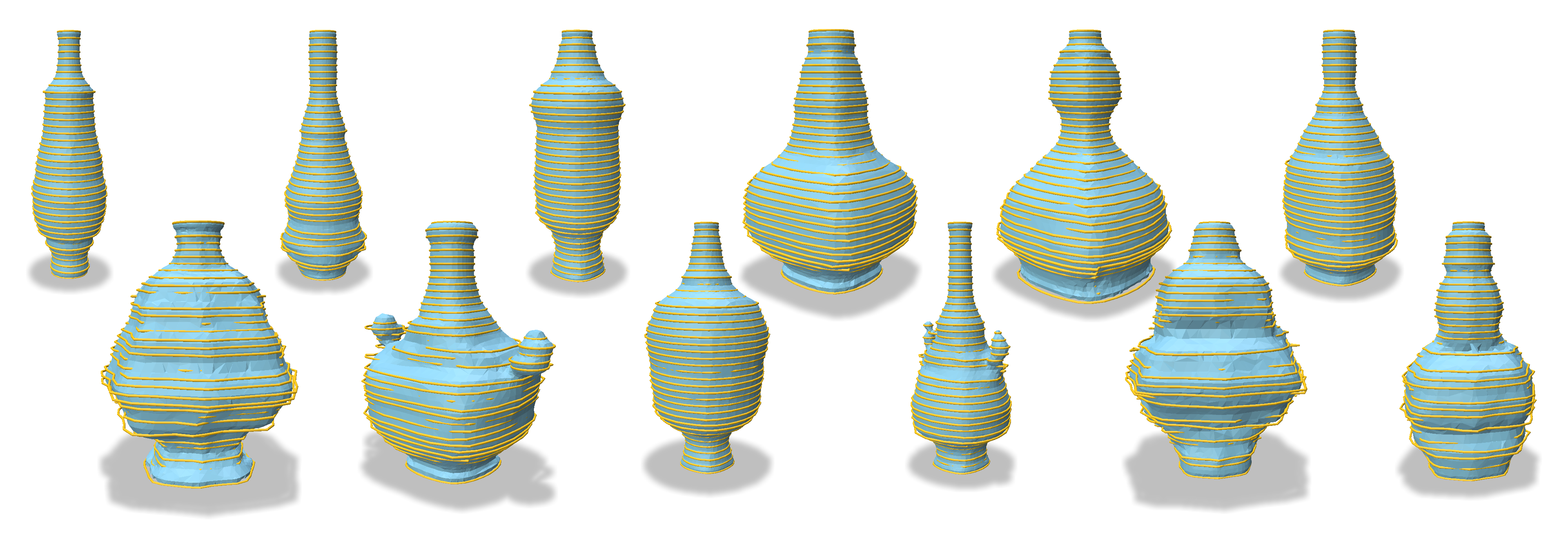
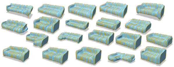
Figure 5: Novel random samples. Without cherry-picking, we sample from the learned latent distribution to generate novel examples which contain varying topologies and sharp features.

3.4 Implementation details

Dataset preparation

To prepare a dataset for training with LoopDraw, we enforce that all meshes are manifold, normalized to unit cube, and are oriented in a semantically consistent way (i.e. all vases are upright along the $y$-axis; all sofas have their length along the $x$-axis). We then select a fixed list of slice planes (we define planes along an axis) whose range and density cover all of the geometry of the input shapes to the extent desired. These slice planes should ideally also be defined such that the same plane should intersect all meshes at roughly the same semantic region, i.e. the first slice plane for a vase dataset should intersect near the bottom of each shape.

End-of-sequence embedding

Since our decoding is autoregressive, the generated time steps should contain information that determines when the sequence generation should terminate. One approach is to enforce (during data pre-processing) a fixed number $k$ of slice planes every mesh in the dataset should intersect. Under this requirement, a loop sequence for a given shape (where the number of loops in the sequence is tied to the shape topology), will contain exactly $k$ level-up flags set to 1, since each level-up flag corresponds to moving up a new plane. Thus, at inference time, we can detect the end of a generated sequence by counting the number of level-up flags set to $1$, and stopping auto-regressive generation once this count reaches the total plane count. This approach makes sense for data that may have similar aspect ratios along the slicing axis (such as vases).

For categories of objects which may have varied aspect ratios, we devise another technique for detecting the end of a sequence. To handle this, our second approach is to define a special end-of-sequence embedding in the training data to be a loop with all features equal to 0 except for a level-up flag of $1$. In this way, we abort the autoregressive generation when the network-predicted loop points are sufficiently close to zero and the level-up flag is $1$. This is analogous to the <EOS> token in language generation models.

KL weight annealing

To facilitate better VAE training, we employ an exponential KL weight annealing schedule similar to the scheme used in [10], in which the weight $\beta_{\text{KL}}$ of the KL divergence loss term is slowly ramped up to the defined value.

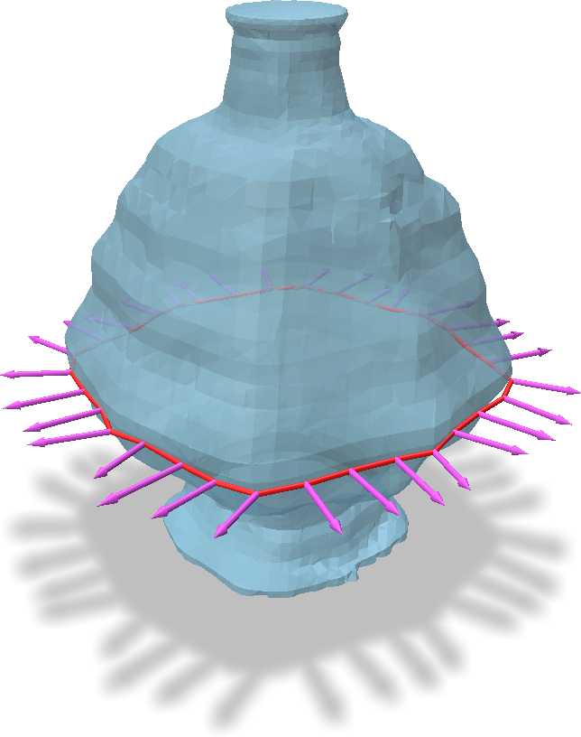
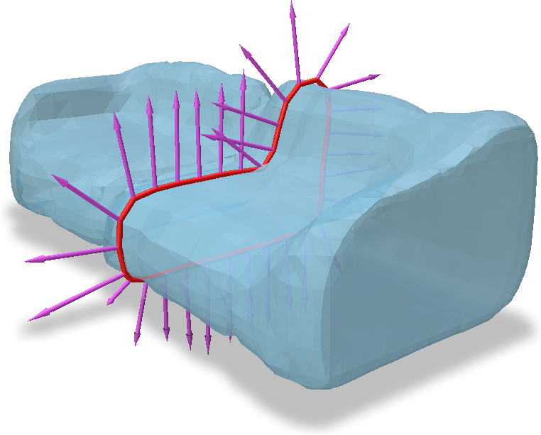
Figure 6: Loop normal estimation.

Reconstructing meshes from loops

All shapes depicted in the figures in our current work are obtained via Poisson reconstruction [16], which we found to be the most reliable method for producing shapes that respect the loop hierarchies and the surface they represent.

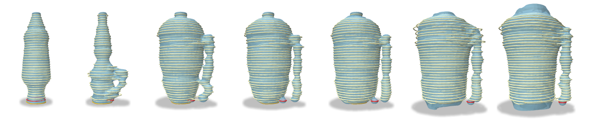
Figure 7: Adaptive shape repair and morphing by the manual editing of a single loop during autoregressive decoding. The original untampered shape is the leftmost figure, showing the original size and position of the target loop in red. The rest of the shapes show decoding results where the target loop (scaled by 0.3) is translated away by increasing amounts (see close-ups in inset figures). To best explain the manually-added anomaly of the shifted loop, the model transitions from decoding a symmetrical, handleless vase to decoding a one-handle vase that accommodates the new target loop position.

Loop-based post-processing heuristics

The interpretability of the loop representation allows employing loop-based post-processing heuristics to obtain better reconstructions from the raw sequence data. To obtain the necessary normals for Poisson reconstruction, we estimate each loop vertex’s normal based on the boundary conditions and line-of-sight (Fig. 6). Loops contained within a larger loop in the same plane (representing inner surfaces), can be assigned inwards-facing normals by testing containment of points within the larger contour.

To prevent holes in the reconstruction from an oriented point cloud, we also sample points in the area enclosed by the top and bottom loops; these points’ normals are set to be the same as the plane normal (for the topmost loop) or its negative (for the bottom loop). These patches of points form the top and bottom cap (or left and right, if the slice plane axis is horizontal) of each shape when reconstructed.

4 Experiments

In this section, we evaluate our method using several qualitative and quantitative experiments. We explore the learned latent space generative capabilities and smoothness properties in Sec. 4.1. Moreover, we demonstrate manual loop editing and intervention possibilities in Sec. 4.2. Finally, we run comparisons in Sec. 4.3 against existing alternative representations for 3D synthesis.

We demonstrate our model’s capabilities on datasets of two shape categories: vases from COSEG [27] and sofas from ShapeNet [5]. We chose these due to their regularity and varied topologies (vases) and sharp features (sofas). For each dataset, we fix a set of slice planes that best captures the geometry: the slice planes for COSEG vases are perpendicular to the $y$ axis, and ShapeNet sofas the positive $x$ axis. For the COSEG vase dataset, we only train on shapes that cut all 40 defined slice planes. The details of the datasets and their slice planes used are in Table 1. In both datasets, we resample every sliced cross-section to $N=32$ vertices per closed polygonal loop. We train using the Adam optimizer with a learning rate of $0.00007$ for 70 epochs followed by a linear ramp-down LR schedule for 7230 epochs ending at zero learning rate. For the COSEG dataset, we use a batch size of 4, with 4 transformer layers (single-head), a layer embedding size of 512, a fully-connected layer size of 512, and latent $\mathbf{z}$ prediction/$\mathbf{d}$ prediction MLPs with a single hidden layer of size 128. For the ShapeNet sofa dataset, we use a batch size of 16, with 8 transformer layers (each with 8 heads), a layer embedding size of 512, a fully-connected layer size of 768, and latent $\mathbf{z}$ prediction/$\mathbf{d}$ prediction MLPs with two hidden layers of size 128. Both models employ a latent code size of $N_{z}=64$.

Table 1: Details of the datasets and slice planes used

Dataset	Train size	# planes	max. seq. length
COSEG vases	223	40	135
ShapeNet sofas	2644	32	121

4.1 Learned Latent Space Properties

We demonstrate that a trained model has a smooth latent space that represents a good distribution of shapes. Fig. 5 shows shapes obtained by sampling random latent vectors $\mathbf{z}$ from the standard normal distribution (for all models trained on each category, the latent size $N_{z}$ is $64$.) The sampled geometries contain varyied topologies (handles on vases), sharp features (armrests and surfaces of sofas), and diverse cross-section shapes throughout.

Fig. 8 shows progressions of shapes obtained by decoding latent vectors linearly interpolating between two points in the latent space. We show that interpolation produces intermediate shapes that are sensible with respect to the dataset and smoothly transition between the start and end shapes. In particular, we note that topology differences imply distinct sequence token differences in LoopDraw’s representation. As a result, interpolating between shapes with similar geometry but differing topology creates sharp delineations between structural configurations. By contrast, implicit representations tend to produce persistent floating artifacts in their in-between shapes.

4.2 Loop Editing and Intervention

The autoregressive shape prior learned in our decoder through the loop representation grants a multitude of possibilities for interpreting and modifying loop sequences during decoding to obtain manual control and refinement.

Basic editing

One such experiment is to apply simple edits—translations and scaling—to certain loops (i.e. time steps in a sequence) before they are autoregressively appended into the input sequence for the prediction of the next time step. Our model shows an ability to adapt the overall generated shape to best explain such manually-added changes, thereby re-contextualizing user edits in semantically reasonable ways. We demonstrate this in Figure 7, where we show continuation shapes resulting from translating one selected loop progressively away from its original location.

Shape blending via loop transplantation

In this task, we intervene in the autoregressive unfolding of a loop sequence by replacing the generated output at certain time steps with a few manually-provided loops from elsewhere (i.e., taken from another shape’s loops, or drawn by hand), and resuming the autoregressive decoding with the edit present.

We demonstrate in Figs. 1 and 4 that this editing method is able to produce meaningful sequence continuations that in effect create “blend shapes”, re-interpreting the same “recipient” shape’s latent code but with cross-sectional characteristics from the “donor” loops.

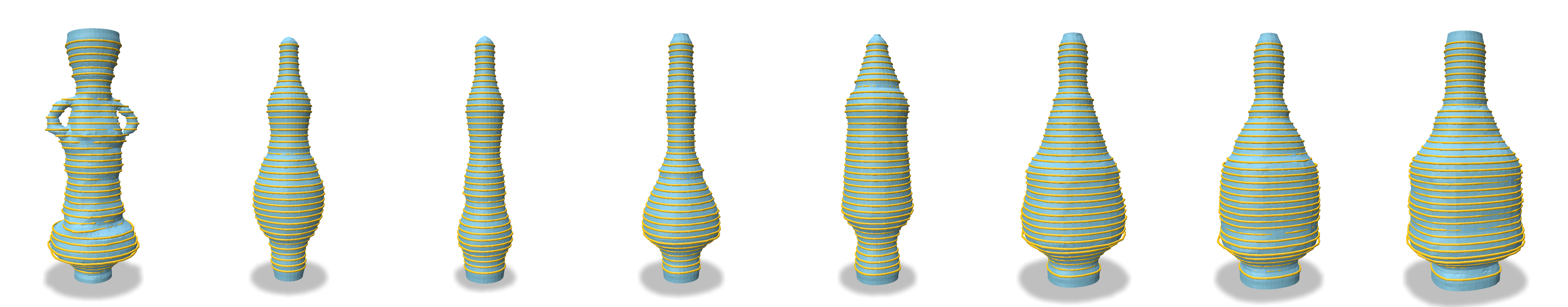
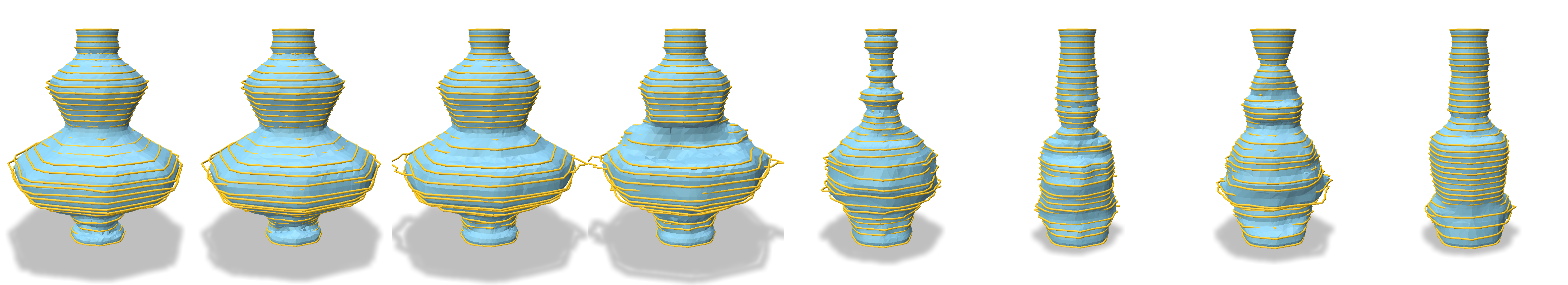
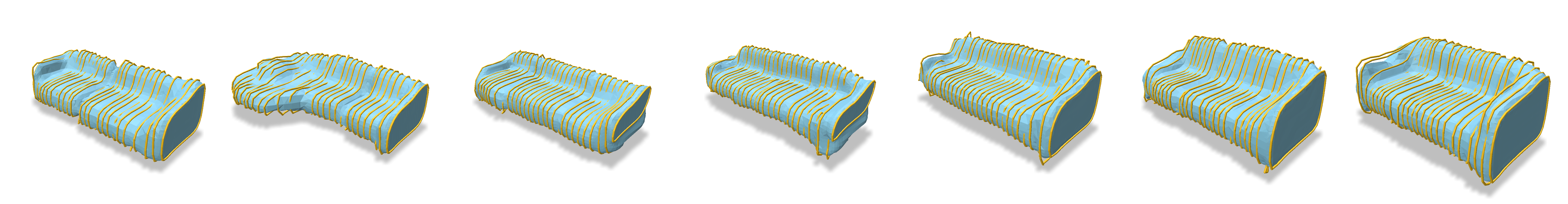
Figure 8: Latent space interpolation for LoopDraw is smooth, while still preserving sharp features and changes in topology.

4.3 Comparisons

Quantitative evaluation

As far as we are aware, LoopDraw is the first technique to use an autoregressive loop primitive for shape synthesis and editing. Since existing techniques take as input alternative representations (such as point clouds, voxels, or tetrahedra), our evaluations inevitably compare across VAEs with different input types. Thus, we compare against various other representations used for generating 3D shapes: Occupancy Networks [21], which represents surfaces with occupancy fields; the VAE variant of ShapeGAN [19] (for encoding capability), which uses signed distance fields as its decoder shape representation; and TetGAN [8], which is a volumetric representation, in Tab. 2. The reconstruction tests evaluate the average Chamfer distance between ground truth shapes and the reconstructed shapes, sampled as point clouds. The FID tests evaluate the FID-based distance between a test set and a batch of 250 random samples, utilizing deep features from a pre-trained PointNet [25] classification network.

We evaluate the metrics for our method on two different surface measures. The first measure compares the fit of our predicted loops compared against loops from the reference set. The second measure reconstructs a surface using Poisson reconstruction and then compares the surface against the underlying surfaces from the reference set. Our results show that, in addition to the interpretability and editability of loops, LoopDraw’s reconstruction and FID performance are on par with the other representations tested.

Qualitative comparisons

Figure 9: Visual results for the Sofas category from our quantitative comparison in Tab. 2. We compare our random samples of sofas with samples from the other three methods trained on the same dataset.

Figure 10: Visual results for the Vases category from our quantitative comparison in Tab. 2. We compare our random samples of vases with samples from the other three methods trained on the same dataset.

We gather random samples from each method trained on the COSEG vase and ShapeNet sofa datasets (Figs. 9 and 10). We note that LoopDraw’s visual quality and structural variety are competitive with these volumetric and implicit surface methods. In particular, both ours and Occupancy Networks strike a similar balance between visual quality and geometric diversity, despite differing in their FID scores. Our results also show features (e.g., indents resembling separate cushions on a sofa) not well-captured by the other methods.

Category	Method	Reconstruction $\downarrow$	FID $\downarrow$
Vases	Occupancy Net.	0.0187	7.42
	ShapeGAN (VAE)	0.0048	20.51
	TetGAN	0.0055	2.57
	Ours (loops-only)	0.0145	3.00
	Ours (reconstructed)	0.0149	5.46
Sofas	Occupancy Net.	0.0118	1.54
	ShapeGAN (VAE)	0.0018	8.30
	TetGAN	0.0024	3.35
	Ours (loops-only)	0.0112	5.48
	Ours (reconstructed)	0.0109	8.77

Table 2: FID and reconstruction evaluation for the three shape categories, with comparisons to other methods.

5 Discussion and Future Work

We presented LoopDraw, an alternative neural representation for synthesizing shapes based on a sequence of cross-sectional contours. This representation is light-weight, flexible, and explicit, capable of representing sharp features and surfaces with varied topology. Since loops are explicit, they can be directly encoded into latent vectors using the proposed loop-encoder. Our auto-regressive decoder produces a series of sequential loops that are interpretable and intuitively editable, which altogether describe the entire shape.

Currently, our system only considers cross-sectional contours along a single axis; however, an interesting direction for future work is to slice and fuse loops across multiple axes. In addition, not all shape categories possess a natural axis and direction in which to scan slice planes; alternative formulations that treat sets of closed loops as unordered in space may be more appropriate for such situations. Finally, we are also interested in exploring other neural applications of loops, such as for surface reconstruction.

6 Acknowledgements

This work was supported in part by the TRI University 2.0 program, the AFOSR MADlab Center of Excellence, as well as gifts from Adobe Research. We are grateful for the AI cluster resources, services, and staff expertise at the University of Chicago. We thank Xiao Zhang and the members of PALS and 3DL for their helpful comments, suggestions, and insightful discussions.

References

- [1] Gill Barequet and Amir Vaxman. Reconstruction of multi-label domains from partial planar cross-sections. In Computer Graphics Forum, volume 28, pages 1327–1337. Wiley Online Library, 2009.
- [2] Amit Bermano, Amir Vaxman, and Craig Gotsman. Online reconstruction of 3d objects from arbitrary cross-sections. ACM Transactions on Graphics (TOG), 30(5):1–11, 2011.
- [3] Jean-Daniel Boissonnat and Pooran Memari. Shape reconstruction from unorganized cross-sections. In Symposium on geometry processing, pages 89–98, 2007.
- [4] Marcel Campen, David Bommes, and Leif Kobbelt. Dual loops meshing: quality quad layouts on manifolds. ACM Transactions on Graphics (TOG), 31(4):1–11, 2012.
- [5] Angel X. Chang, Thomas Funkhouser, Leonidas Guibas, Pat Hanrahan, Qixing Huang, Zimo Li, Silvio Savarese, Manolis Savva, Shuran Song, Hao Su, Jianxiong Xiao, Li Yi, and Fisher Yu. ShapeNet: An Information-Rich 3D Model Repository. Technical Report arXiv:1512.03012 [cs.GR], Stanford University — Princeton University — Toyota Technological Institute at Chicago, 2015.
- [6] Zhiqin Chen and Hao Zhang. Learning implicit fields for generative shape modeling. CoRR, abs/1812.02822, 2018.
- [7] Xianzhong Fang, Mathieu Desbrun, Hujun Bao, and Jin Huang. Topocut: Fast and robust planar cutting of arbitrary domains. ACM Trans. Graph., 41(4), jul 2022.
- [8] William Gao, April Wang, Gal Metzer, Raymond A Yeh, and Rana Hanocka. Tetgan: A convolutional neural network for tetrahedral mesh generation. arXiv preprint arXiv:2210.05735, 2022.
- [9] Kunal Gupta and Manmohan Chandraker. Neural mesh flow: 3d manifold mesh generation via diffeomorphic flows. In Proceedings of the 34th International Conference on Neural Information Processing Systems, NIPS’20, Red Hook, NY, USA, 2020. Curran Associates Inc.
- [10] David Ha and Douglas Eck. A neural representation of sketch drawings. In ICLR 2018, 2018. 2018.
- [11] Rana Hanocka, Amir Hertz, Noa Fish, Raja Giryes, Shachar Fleishman, and Daniel Cohen-Or. Meshcnn: A network with an edge. ACM Trans. Graph., 38(4):90:1–90:12, July 2019.
- [12] Rana Hanocka, Gal Metzer, Raja Giryes, and Daniel Cohen-Or. Point2mesh: A self-prior for deformable meshes. ACM Trans. Graph., 39(4), aug 2020.
- [13] Zekun Hao, Hadar Averbuch-Elor, Noah Snavely, and Serge Belongie. Dualsdf: Semantic shape manipulation using a two-level representation. pages 7631–7641, 2020.
- [14] Amir Hertz, Rana Hanocka, Raja Giryes, and Daniel Cohen-Or. Deep geometric texture synthesis. ACM Trans. Graph., 39(4), 2020.
- [15] R. Kenny Jones, Theresa Barton, Xianghao Xu, Kai Wang, Ellen Jiang, Paul Guerrero, Niloy Mitra, and Daniel Ritchie. Shapeassembly: Learning to generate programs for 3d shape structure synthesis. ACM Transactions on Graphics (TOG), Siggraph Asia 2020, 39(6):Article 234, 2020.
- [16] Michael Kazhdan, Matthew Bolitho, and Hugues Hoppe. Poisson surface reconstruction. In Proceedings of the fourth Eurographics symposium on Geometry processing, volume 7, 2006.
- [17] Nasser Kehtarnavaz, L Ray Simar, and Rui JP de Figueiredo. A syntactic/semantic technique for surface reconstruction from cross-sectional contours. Computer vision, graphics, and image processing, 42(3):399–409, 1988.
- [18] Diederik P. Kingma and Max Welling. Auto-encoding variational bayes. In Yoshua Bengio and Yann LeCun, editors, 2nd International Conference on Learning Representations, ICLR 2014, Banff, AB, Canada, April 14-16, 2014, Conference Track Proceedings, 2014.
- [19] Marian Kleineberg, Matthias Fey, and Frank Weichert. Adversarial generation of continuous implicit shape representations. arXiv preprint arXiv:2002.00349, 2020.
- [20] Hsueh-Ti Derek Liu, Vladimir G. Kim, Siddhartha Chaudhuri, Noam Aigerman, and Alec Jacobson. Neural subdivision. ACM Trans. Graph., 39(4), 2020.
- [21] Lars Mescheder, Michael Oechsle, Michael Niemeyer, Sebastian Nowozin, and Andreas Geiger. Occupancy networks: Learning 3d reconstruction in function space. In Proceedings of the IEEE/CVF conference on computer vision and pattern recognition, pages 4460–4470, 2019.
- [22] Gal Metzer, Rana Hanocka, Denis Zorin, Raja Giryes, Daniele Panozzo, and Daniel Cohen-Or. Orienting point clouds with dipole propagation. ACM Trans. Graph., 40(4), jul 2021.
- [23] Charlie Nash, Yaroslav Ganin, S. M. Ali Eslami, and Peter W. Battaglia. Polygen: An autoregressive generative model of 3d meshes. ICML, 2020.
- [24] Jeong Joon Park, Peter Florence, Julian Straub, Richard Newcombe, and Steven Lovegrove. Deepsdf: Learning continuous signed distance functions for shape representation. In The IEEE Conference on Computer Vision and Pattern Recognition (CVPR), June 2019.
- [25] Charles R Qi, Hao Su, Kaichun Mo, and Leonidas J Guibas. Pointnet: Deep learning on point sets for 3d classification and segmentation. In Proceedings of the IEEE conference on computer vision and pattern recognition, pages 652–660, 2017.
- [26] Ashish Vaswani, Noam Shazeer, Niki Parmar, Jakob Uszkoreit, Llion Jones, Aidan N. Gomez, Łukasz Kaiser, and Illia Polosukhin. Attention is all you need. In Proceedings of the 31st International Conference on Neural Information Processing Systems, NIPS’17, page 6000–6010, Red Hook, NY, USA, 2017. Curran Associates Inc.
- [27] Yunhai Wang, Shmulik Asafi, Oliver Van Kaick, Hao Zhang, Daniel Cohen-Or, and Baoquan Chen. Active co-analysis of a set of shapes. ACM Transactions on Graphics (TOG), 31(6):1–10, 2012.
- [28] Rundi Wu, Chang Xiao, and Changxi Zheng. DeepCAD: A deep generative network for computer-aided design models. 2021.
- [29] Zhirong Wu, Shuran Song, Aditya Khosla, Fisher Yu, Linguang Zhang, Xiaoou Tang, and Jianxiong Xiao. 3d shapenets: A deep representation for volumetric shapes. In Proceedings of the IEEE conference on computer vision and pattern recognition, pages 1912–1920, 2015.
- [30] Jie Yang, Kaichun Mo, Yu-Kun Lai, Leonidas J Guibas, and Lin Gao. Dsg-net: Learning disentangled structure and geometry for 3d shape generation. ACM Transactions on Graphics (TOG), 2022.
- [31] Yun Zeng, Dimitris Samaras, Wei Chen, and Qunsheng Peng. Topology cuts: A novel min-cut/max-flow algorithm for topology preserving segmentation in n–d images. Computer vision and image understanding, 112(1):81–90, 2008.
- [32] Yixin Zhuang, Ming Zou, Nathan Carr, and Tao Ju. Anisotropic geodesics for live-wire mesh segmentation. In Computer Graphics Forum, volume 33, pages 111–120. Wiley Online Library, 2014.
- [33] Ming Zou, Michelle Holloway, Nathan Carr, and Tao Ju. Topology-constrained surface reconstruction from cross-sections. ACM Transactions on Graphics (TOG), 34(4):128, 2015.