Basis set generation and optimization in the NISQ era with Quiqbox.jl

Abstract

In the noisy intermediate-scale quantum era, ab initio computation of the electronic structure problem has become one of the major benchmarks for identifying the boundary between classical and quantum computational power. The single-particle basis set plays a key role in the electronic structure methods implemented on both classical and quantum devices. To investigate the consequences of the single-particle basis set, we propose a framework for more customizable basis set generation and basis set optimization. This framework allows configurations of composite Gaussian-type basis functions to go beyond typical Gaussian-type basis set frameworks such as the atomic orbitals and floating basis sets. Such basis set generations set the stage for more flexible variational optimization of basis set parameters. To realize this framework, we have developed an open-source electronic structure package named ‘‘Quiqbox’’ in the Julia programming language. Both the Hartree--Fock procedure and Gaussian-based electronic integral computations are implemented in this package. We compare Quiqbox with the basis set optimization package DiffiQult and find faster convergence of the basis set optimization with lower run time. We also demonstrate the additional customizability Quiqbox brings for more systematic basis set research with an example of constructing and optimizing delocalized orbitals.

I Introduction

Electronic structure [1, 2] has been the intersection among multiple disciplines, including quantum physics, quantum chemistry, and material science. The goal of the field is to study the states and dynamics of many-electron systems, or more specifically, the electronic Hamiltonian [1] determined by a nuclear field. Consider a quantum system consisting of $N$ electrons and $N^{\prime}$ nuclei, in which the $a^{\prime}$th nucleus with charge $Z_{a^{\prime}}$ is located on position ${\bm{R^{\prime}_{a^{\prime}}}}$. The information of all the nuclei forms a set that specifies the nuclear field of the system:

$$\mathbb{M}\equiv\{({\bm{R^{\prime}_{a^{\prime}}}},Z_{a^{\prime}})\,|\,a^{\prime}\!=\!1,\dots,N^{\prime}\}.$$ (1)

The electronic Hamiltonian of this system can be separated from its total Hamiltonian $H_{\rm tot}$ when the Born-Oppenheimer approximation is applied:

$$H_{\rm elec}(\mathbb{M};N^{\uparrow},N^{\downarrow})=H_{\rm tot}(\mathbb{M};N)-H_{\rm nuc}(\mathbb{M})$$ (2)

where $N^{\uparrow}$ and $N^{\downarrow}$ are the number of spin-up electrons and spin-down electrons, respectively, such that $N\!=\!N^{\uparrow}\!+\!N^{\downarrow}$, and $H_{\rm nuc}$ is the sum of the nuclear kinetic energy and nuclear-nuclear repulsion energy. Instead of being the direct sum of single-electron Hamiltonians, $H_{\rm elec}$ (in the Hartree atomic units) has the form:

$$H_{\rm{elec}}(\mathbb{M};N^{\uparrow},N^{\downarrow})$$ (3)

$$= \sum_{a=1}^{N}(-\frac{1}{2}\nabla_{\bm{A}}^{2}-\sum_{a^{\prime}=1}^{N^{\prime}}\frac{Z_{a^{\prime}}}{|\bm{r_{a}}-\bm{R^{\prime}_{a^{\prime}}}|})+\sum_{a=1,b>a}^{N,N}\frac{1}{|\bm{r_{a}}-\bm{r_{b}}|}$$

$$\equiv \sum_{a}h_{1}(a;\,\mathbb{M})+\sum_{b>a}h_{2}(a,b)$$

where $h_{1}(a;\,\mathbb{M})$ is the one-electron operator that represents the kinetic energy of the $a$th electron and the Coulomb attraction between it and the nuclei in the system; $h_{2}(a,b)$ is the two-electron operator that represents the interaction between the $a$th and $b$th electrons.

One of the basic goals of electronic structure study is to solve the eigenvalue problem of the electronic problem:

$$H_{\rm elec}\Phi_{n}=\mathcal{E}_{n}\Phi_{n}$$ (4)

where $\Phi_{n}$ is the eigenfunction corresponding to the $n$th eigenenergy $\mathcal{E}_{n}$. $\Phi_{n}$ is a many-electron wavefunction that obeys the anti-symmetric constraint for identical fermions.

In an effort to alleviate the exponentially growing computational cost with respect to the total number of electrons, various ansatzes and numerical optimizations for the many-electron eigenfunctions have been proposed. Within the domain of classical numerical simulation, mean-field methods such as the Hartree--Fock method [1, 3, 4] were proposed to approximate the ground state with a non-interacting fermionic state (i.e., a single Slater determinant state), while post-Hartree--Fock methods [1, 5, 6, 7] try to further represent the ground state with the superposition of Slater determinant states based on one reference state (Hartree--Fock state) or multiple reference states.

With the successful demonstration on a quantum device to solve for the ground state of He--$\rm{H^{+}}$ [8], variational quantum eigensolver (VQE) has established its potential in utilizing noisy intermediate-scale quantum (NISQ) devices [9, 10] for calculating electronic structure [11, 12, 13, 14]. However, due to the limited scale of NISQ devices, the applicable basis sets to perform qubit encoding for VQE have been restricted to small-size basis sets [14]. On the other hand, the interest around basis set optimization for electronic structure has grown recently [15, 16, 17] with the development of computer algebra techniques such as automatic differentiation (AD) [18, 19].

In this paper, we propose a framework for customizing and optimizing composite basis sets based on Gaussian-type orbital (GTO). This is realized by the open-source software toolkit we developed in the Julia programming language [20, 21]: Quiqbox.jl v0.5.2 (Quiqbox) [22].

We believe that a unified control and comparable design of basis sets play a crucial role in developing and benchmarking electronic structure algorithms in the present NISQ era when the exploration of the boundary between classical and quantum computational power is important for exploring practical quantum primacy [9, 23, 24]. We show that with the help of Quiqbox, one can control, modify, and improve the existing Gaussian basis sets composed of atomic orbitals (AOs), which are used to form a linear combination of atomic orbitals (LCAO) as a localized molecular orbital. Moreover, one can also construct and optimize more general basis sets beyond AOs, which outperform typical Gaussian basis sets or achieve similar performance while meeting specific requirements such as minimal basis set size.

The paper is organized as follows. In Sec. II, we elaborate on the proposal to carry out a more systematic study of basis set design in the NISQ era. In Sec. III, we describe the additional freedom our composite basis set generation framework brings for general electronic structure algorithms. We then derive the general expression of the basis set parameter gradient under the said framework and explain Quiqbox’s specialized optimization architecture in Sec. IV, followed by comparison and benchmarking against existing packages in Sec. V. In Sec. VI, we demonstrate an example of using Quiqbox to construct basis sets with exotic properties. We conclude the paper and discuss the outlook of Quiqbox’s development in Sec. VII. Additionally, we include tables to summarize all the essential acronyms and notation conventions we use throughout this paper in the Appendix (Sec. IX).

II Basis set design for the NISQ era

Let $E_{0}$ be the approximate ground-state energy of $H_{\rm elec}$ associated with a quantum many-electron system. Given an non-orthogonal basis set $\{\phi_{n}\,|\,n=1,\dots,W\}$ that contains $W$ spatial orbitals with an overlap matrix $\bm{S}$ defined by $S_{ij}=\braket{\phi_{i}}{\phi_{j}}$, we can construct an orthonormal basis set

$$\{\varphi_{m}\,|\,\braket{\varphi_{i}}{\varphi_{j}}=\delta_{ij},m=1,\dots,W\},$$ (5)

by performing a symmetric orthogonalization

$$\varphi_{m}=\sum_{n}X_{nm}\phi_{n},\;{\rm{with}}\;\bm{X}\equiv\bm{S}^{1/2}.$$ (6)

Thus, a trial state $\ket{\Psi_{0}(\bm{c})}$ parameterized by $\bm{c}$ can be constructed from $\{\varphi_{m}\}$ following an ansatz of the ground state. Depending on the selected ansatz, $\bm{c}$ may not only characterizes the single-electron modes but also contains the amplitudes of multiple Slater determinant states formed by the modes. According to the variational principle, $E_{0}$ would be the lower bound of the energy expectation $\tilde{E_{0}}(\bm{c})$ with respect to $\ket{\Psi_{0}(\bm{c})}$:

$$E_{0}\leq\tilde{E_{0}}(\bm{c})=\frac{\braket{\Psi_{0}(\bm{c})}{H_{\rm elec}}{\Psi_{0}(\bm{c})}}{\braket{\Psi_{0}(\bm{c})}{\Psi_{0}(\bm{c})}}.$$ (7)

Regardless of the choice of ansatz (e.g., the Hartree--Fock approximation) used to construct $\ket{\Psi_{0}(\bm{c})}$, $\tilde{E_{0}}(\bm{c})$ in Eq. (7) can always be decomposed into three parts:

$$\quad\bm{x} =\bm{f_{1}}({\bm{A}}[\{\varphi_{m}\}]),$$ (8)

$$\quad\bm{y} =\bm{f_{2}}({\bm{B}}[\{\varphi_{m}\}]),$$

$$\tilde{E_{0}}(\bm{c}) =f_{3}(\bm{c};\,\bm{x},\,\bm{y}),$$

where vector functions $\bm{f_{1}}$: $\mathbb{R}^{W^{2}}\!\to\!\mathbb{R}^{W^{\prime}}$ and $\bm{f_{2}}$: $\mathbb{R}^{W^{4}}\!\to\!\mathbb{R}^{W^{\prime\prime}}$ generate intermediate results $\bm{x}$ and $\bm{y}$ mapped from tensor ${\bm{A}}$ and tensor ${\bm{B}}$ which discretize the one-electron and two-electron operators respectively onto $\{\varphi_{m}\}$. The tensor elements of ${\bm{A}}$ and ${\bm{B}}$ are called electronic integrals (or molecular integrals in the context of molecular systems):

$$\begin{split}A_{mn}&=\int d\bm{r_{a}}\varphi_{m}^{*}(\bm{r_{a}})h_{1}(a;\,\mathbb{M})\varphi_{n}(\bm{r_{a}})\\ &\equiv(\varphi_{m}|\varphi_{n}),\end{split}$$ (9)

$$\begin{split}B_{mnpq}&=\int d\bm{r_{a}}d\bm{r_{b}}\varphi_{m}^{*}(\bm{r_{a}})\varphi_{p}^{*}(\bm{r_{b}})h_{2}(a,b)\varphi_{q}(\bm{r_{b}})\varphi_{n}(\bm{r_{a}})\\ &\equiv(\varphi_{m}\varphi_{n}|\varphi_{p}\varphi_{q}).\end{split}$$ (10)

The third mapping function $f_{3}$ in Eq. (8) takes t$\bm{x}$ and $\bm{y}$ as parameters, and $\bm{c}$ as the input variable. In this way, the calculation of $E_{0}$ is transformed into an optimization problem of finding the optimal value of $\bm{c}$:

$$\bm{c^{0}}=\underset{\bm{c}}{{\rm arg}\,{\rm min}}\,\tilde{E_{0}}(\bm{c}).$$ (11)

This can be done using either a self-consistent field (SCF) method [1, 25, 26, 27], or a gradient-based method realized by AD [28], as the optimizer of $\bm{c}$.

One can see from Eq. (8) that the expression of $\bm{f_{1}}$, $\bm{f_{2}}$, and $f_{3}$ depend on the choice of the ground state ansatz. More specifically, elements of $\bm{x}$ and $\bm{y}$ can be considered as the portions of ground-state energy contributed by single-Slater determinant states. Thus, for a multi-configuration ansatz, $W^{\prime}$ and $W^{\prime\prime}$ would both be larger than one, as opposed to Hartree--Fock methods. Consequently, the vector space of $\bm{c}$ will be larger to presumably contain a better approximation of the true ground-state energy $\mathcal{E}_{0}$, which generally also makes it harder for the optimizer to find $\bm{c^{0}}$. An example of $\bm{f_{1}}$, $\bm{f_{2}}$ and $f_{3}$’s expression in the case of restricted Hartree--Fock as the applied electronic structure algorithm is shown in Eq. (26) in Sec. IV.1 where we show the analytical differentiation process implemented in Quiqbox.

Eqs. (9) and (10) indicate that the discretization of $H_{\rm elec}$ is affected by the choice of $\{\varphi_{m}\}$, which can not only introduce error due to the incompleteness of finite basis set but also affect the hardness of the electronic structure problem [29]. Following Eqs. (8--11), the process of solving for the electronic structure properties, such as the ground-state energy, can be generalized into a standard procedure shown in FIG. 1(a). The electronic Hamiltonian of the system of interest is first discretized by a finite set of basis functions. After that, based on a model ansatz, a further approximation is applied (usually about the many-electron wavefunction) to construct the algebraic expression for the desired observable as an objective function (i.e., the ground-state energy) with respect to the discretized Hamiltonian. Thus, the objective function is implicitly a functional of the basis set. Finally, a numerical eigensolver (typically a variational optimizer) finds the approximate solution $\bm{c^{0}}$. Accordingly, the procedure of VQE for molecular electronic structure also falls into four similar steps as shown in FIG. 1(b).

(a) The general steps of solving a many-electron system.

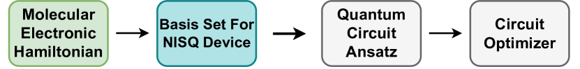
(b) Applying VQE to the electronic structure problem of molecular systems.

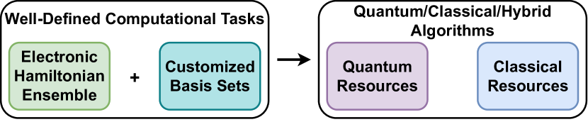
(c) Using basis set design and molecular ensemble to construct well-defined computational tasks for NISQ or classical algorithms.

Figure 1: The overall procedure of solving the electronic Hamiltonian can be split into four steps for both classical and quantum algorithms as shown in FIG. 1(a) and FIG. 1(b). A more systematic design and optimization of basis sets can aid the development of these algorithms for electronic structure problems, as shown in FIG. 1(c).

From the generalized procedure of solving an electronic Hamiltonian, we explained the effect that a basis set has on both computational accuracy and resources. In the context of using VQE for electronic structure, this effect becomes more significant. Due to the limited number of qubits in NISQ devices for fermionic encoding [30, 31, 32], there is often a trade-off between the size of the basis set and the size of the studied many-electron systems [7, 33]. Moreover, the applied Gaussian-based AOs (e.g., STO-3G [34], cc-pVDZ [35]) are, in fact, not fully optimized to minimize electronic structure properties such as the ground state energy given a fixed number of single-electron modes. This can be supported by the literature about the optimization of AOs [36, 16]. For the purpose of improving the practicality of using NISQ algorithms to solve electronic structure problems, we believe the systematic study of customizable basis set generation is of high importance. For instance, including basis set optimization and design as part of VQE’s architecture can introduce the physical characteristics of many-electron systems in real space for VQE. This can potentially improve various aspects of the algorithm, such as trial qubit state preparation or optimizer configuration for the landscape of the corresponding parameter space.

Additionally, customizable basis set generation enables a better formulation of studying the electronic Hamiltonian as a computational task. It has been shown that approximating the ground state of the electronic Hamiltonian with a fixed basis set in real space (and fixed particle number) is QMA-complete [29, 37]. This suggests that the way a basis set discretizes the real space can affect the hardness of the electronic structure problem. We can further incorporate this idea into basis set designs. Given an ensemble of electronic Hamiltonians with the same electron number, by designing customized basis sets, we shall generate instances of electronic structure problems classified by different computational complexities (see FIG. 1(c)). Not only does this help study the complexity of electronic Hamiltonians, but it also provides another metric for benchmarking the capability of quantum simulation algorithms (or hybrid algorithms that rely on quantum resources too) [38, 39, 33, 40, 41, 23] against pure classical approaches.

III More freedom in Gaussian basis set design

The basis sets used in electronic systems typically can be classified into three main categories: delocalized basis sets that rely on periodic functions like plane waves as basis functions [42, 43], real-space basis sets that use localized functions such as wavelets distributed on grid points [44, 45, 46], and Gaussian basis sets that utilize GTO to form contracted functions to approximate Slater-type orbitals [47, 48].

We also utilize GTO as the building block of more complicated basis functions for several reasons. First and foremost, GTO currently is one of the common choices for constructing basis set for molecular systems, the scale of which is applicable to VQE in the current state of NISQ devices [8, 7, 14]. This allows us to optimize and build new basis sets on the existing progress of GTO research. Secondly, the orbital integrals in Eqs. (9) and (10) in the case of GTO can be calculated analytically for the most part [49, 50], making the numerical error of the tensor elements of the discretized electronic Hamiltonian easily controlled. Last but not least, with proper manipulations of Gaussian functions, various Gaussian-based basis sets with different features from AOs, such as floating Gaussian basis sets [51, 52, 53], Gaussian-based real-space basis sets [54, 55], and even-tempered basis sets [56], can also be constructed.

By careful design, the variety of basis functions built from GTO can be greatly improved compared to existing Gaussian basis set generation methods in the standard software packages such as PySCF [57] and Psi4 [58]. In this section, we will formally introduce GTO (Gaussian-type orbital). Then, we focus on describing the proposed framework that provides extra freedom in using GTO to build composite basis functions that improve the customizability of Gaussian-based basis sets.

In general, the form of a GTO in Cartesian coordinates can be expressed as

$$\phi^{\rm{GTO}}(\bm{r};\bm{R},\mathpzc{i},\mathpzc{j},\mathpzc{k},\alpha)$$ (12)

$$\,\equiv\, N(x\!-\!X)^{\mathpzc{i}}(y\!-\!Y)^{\mathpzc{j}}(z\!-\!Z)^{\mathpzc{k}}{\rm{exp}}(-\alpha|\bm{r\!-\!R}|^{2}),$$

$$\mathpzc{l} \,\equiv\, \mathpzc{i}+\mathpzc{j}+\mathpzc{k},\quad\bm{r}\,\equiv\,[x,\,y,\,z],\quad\bm{R}\,\equiv\,[X,\,Y,\,Z],$$

where $\alpha$ is the exponent coefficient that determines how diffused the GTO is, $\mathpzc{l}$ represents the orbital angular momentum, and $\bm{R}$ is the center position of the orbital. The most common use of GTOs is to form a contracted Gaussian-type orbital (CGTO)

$$\phi_{m}^{\rm{CGTO}}(\bm{r};\bm{R_{m}},\mathpzc{i}_{m},\mathpzc{j}_{m},\mathpzc{k}_{m})$$ (13)

$$\equiv \sum_{n}d_{n}\,\phi^{\rm{GTO}}_{n}(\bm{r};\bm{R_{m}},\alpha_{n},\mathpzc{i}_{m},\mathpzc{j}_{m},\mathpzc{k}_{m}).$$

$d_{n}$ are called ‘‘contraction coefficients’’ as multiple concentric GTOs with equal angular momentum and different weights are ‘‘contracted’’ to approximate a Slater-type orbital (STO). STO is a type of orbital that provides an accurate representation of AOs [1]. The function curve of STO has a cusp near the orbital center due to its non-vanishing gradient, which GTO is incapable of reconstructing. However, forming a CGTO with appropriate contraction coefficients instead of a single GTO can alleviate this problem while retaining the computational efficiency of GTO [34]. In our basis set generation framework, a basis function need not be a CGTO composed of concentric GTOs with the same angular momentum but can also be the linear combination of multi-center GTOs that may or may not have the same angular momentum. We define this type of generalized Gaussian-based orbital as mixed-contracted Gaussian-type orbital (MCGTO):

$$\phi_{m^{\prime}}^{\rm{MCGTO}}(\bm{r})\equiv\sum_{m}\phi_{m}^{\rm{CGTO}}(\bm{r};\bm{R_{m}},\mathpzc{i}_{m},\mathpzc{j}_{m},\mathpzc{k}_{m}).$$ (14)

MCGTO provides the first additional freedom in our framework, which makes it possible to construct more delocalized basis functions than a GTO to incorporate the interatomic bonding information before applying the SCF methods. For instance, one can use the molecular orbitals of small systems as the basis functions for larger combined systems.

Primitive variables that correlate multiple CGTOs through customized mapping functions are the second additional freedom to basis set generation. These correlations can have direct physical interpretations. For example, homonuclear diatomic molecules have spatial symmetry that can be described by the point group $D_{\infty h}$, i.e., they have rotational symmetry about their internuclear axis and reflection symmetry about a plane perpendicular to the axis [59]. Such molecular symmetry affects the formation of their molecular orbitals. Therefore, it is reasonable to correlate the parameters of AOs during the AO-based basis set generation so that such symmetry is imposed to reduce the computational cost for later parameter optimization. Taking a step further, by using the primitive variables that correlate basis functions, grid-based Gaussian basis sets become available. In such a scenario, the center position of each basis function would also be the location of a grid point controlled by the spacing of the grid box. A mapping function from the single spacing parameter (i.e., the sparsity of gird points) to the CGTO center positions greatly lower the total number of basis set parameters while maintaining the topology of the grid box. Moreover, the exponent and contraction coefficients of the CGTOs can be correlated to reduce parameters further. One example of such type of basis set is shown in FIG. 2.

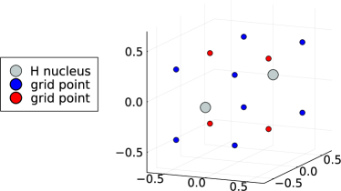
Figure 2: A $1\!\times\!2\!\times\!1$ grid-based Gaussian basis set for $\rm{H_{2}}$. Based on the geometric symmetry of $\rm{H_{2}}$, constraints on CGTO parameters can be imposed. For example, the CGTOs located on the grid points with the same color can have identical exponent and contraction coefficients. Correlated grid points can be directly generated using the helper function GridBox in Quiqbox.

Combining the design of a generalized Gaussian-based orbital, MCGTO, and the additional correlation configuration among CGTO parameters, we complete our design of a more customizable generation of Gaussian-based basis sets. To provide a straightforward comparison between it and the standard basis set generation method, the computational graphs of both methods in the context of electronic ground-state energy computation are shown in FIG. 3.

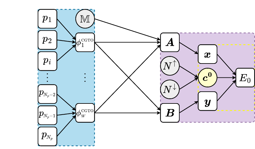
(a) The complete computational graph of an algorithm solving for the electronic ground-state energy in standard electronic structure packages.

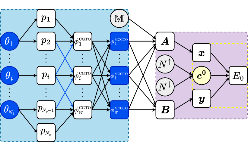
(b) The computational graph with extra connectivity and layers after replacing the standard basis set generation method in FIG. 3(a) with our framework. In the light blue box, the leftmost added layer represents the primitive parameters $\{\theta_{i}\}$ that control CGTO parameters $\{p_{i}\}$ through mapping functions, and the rightmost layer represents MCGTOs as the output basis functions. Additionally, since the CGTOs can share parameters in Quiqbox, more connectivity (blue lines) between the CGTO parameters and CGTOs becomes available.

Figure 3: The comparison between the standard basis set generation method and our framework for finding the electronic ground-state energy. The light blue box represents the basis set construction. The light purple box represents the electronic algorithm to compute the approximate ground-state energy $E_{0}$. The yellow dashed box represents the chosen eigensolver that produces $\bm{c^{0}}$ as the final input to obtain $E_{0}$.

Aside from the common input parameters indicated in Eq. (3), the parameters from the generated basis set $\{\phi_{n}\}$ can be considered the primary parameters that affect $E_{0}$. Specifically, for the standard Gaussian basis set generation method (FIG. 3(a)), only the CGTO parameters $\{p_{i}\,|\,i=1\dots N_{p}\}$ can be the basis set parameters. However, in our basis set generation framework (FIG. 3(b)), such restrictions are lifted by allowing more primitive parameters $\{\theta_{i}\,|\,i=1\dots N_{\theta}\}$ to control the orbital parameters. On top of this, correlations between CGTOs can be implemented with shared orbital parameters among them, and MCGTOs serve as the finally generated basis functions. As we fixed the coefficients generated by the eigensolver as shown in the yellow dashed box (along with other parameters in the grey circled boxes in FIG. 3), $E_{0}$ is mapped from $\{\theta_{i}\}$ through layers of differentiable nodes connected by various mapping functions. Thus, $\{\theta_{i}\}$ as the basis set parameters can be optimized using variational methods based on the analytical gradient of $E_{0}$ with respect to them, which forms the process of basis set optimization.

IV Variational optimization of basis set parameters

IV.1 Generalized analytical electronic structure gradient with respect to basis set parameters

Let $\{\theta_{i}\,|\,\theta_{i}\in\mathbb{R},i=1,\dots,N_{\theta}\}$ be a set of unique real parameters (meaning they are distinguishable from each other by their symbols and indices regardless of whether they have the same value) that $E_{0}$ explicitly or implicitly depends on. To minimize $E_{0}$ with respect to $\{\theta_{i}\}$, we need to calculate the gradient of $E_{0}$ with respect to the vectorized parameters $\bm{\theta}=[\theta_{1},\dots,\theta_{i},\dots,\theta_{N_{\theta}}]^{T}$, the analytical form of which can be expressed as [60, 51]:

$$\frac{dE_{0}}{d\bm{\theta}}=\sum_{m}\frac{\partial E_{0}}{\partial\varphi_{m}}\frac{\partial\varphi_{m}}{\partial\bm{\theta}}+\braket{\Psi_{0}}{\frac{\partial H_{\rm elec}}{\partial\bm{\theta}}}{\Psi_{0}}.$$ (15)

The first term in Eq. (15) represents the explicit dependency of the parameters based on the ground state approximation, and the second term represents the effective force from the Hellmann--Feynman theorem [51, 61]. For the purpose of a systematic basis set optimization, $\{\theta_{i}\}$ represents a set of unique and independent basis set parameters to be optimized. Assuming the electronic Hamiltonian is independent of these parameters (e.g., the basis function centers can be detached from the nuclei locations, forming floating basis functions [51, 52, 53]), the second term in Eq. (15) is eliminated. Thus, the partial derivative of $E_{0}$ with respect to a single basis set parameter $\theta_{i}$ reduces to

$$\frac{\partial E_{0}}{\partial\theta_{i}}=\sum_{m}\frac{\partial E_{0}}{\partial\varphi_{m}}\frac{\partial\varphi_{m}}{\partial\theta_{i}}.$$ (16)

Combining Eq. (16) with Eqs. (8--10), we can derive a more detailed formula of the parameter partial derivative for a general electronic structure algorithm:

$$\frac{\partial E_{0}}{\partial\theta_{i}}= \sum_{j}\frac{\partial E_{0}}{\partial x_{j}}\frac{\partial x_{j}}{\partial\bm{A}}\cdot\frac{\partial\bm{A}}{\partial\theta_{i}}+\sum_{k}\frac{\partial E_{0}}{\partial y_{k}}\frac{\partial y_{k}}{\partial\bm{B}}\cdot\frac{\partial\bm{B}}{\partial\theta_{i}}$$ (17)

$$= \sum_{mn}(\nabla_{\bm{A}}E_{0}\odot\partial_{\theta_{i}}\bm{A})_{mn}+\sum_{mnpq}(\nabla_{\bm{B}}E_{0}\odot\partial_{\theta_{i}}\bm{B})_{mnpq}$$

where $\odot$ denotes element-wise multiplication, and

$$\begin{split}(\nabla_{\bm{A}}E_{0})_{mn}=&(\sum_{j}\frac{\partial E_{0}}{\partial x_{j}}\frac{\partial x_{j}}{\partial\bm{A}})_{mn},\end{split}$$ (18)

$$\begin{split}(\nabla_{\bm{B}}E_{0})_{mnpq}=&(\sum_{k}\frac{\partial E_{0}}{\partial y_{k}}\frac{\partial y_{k}}{\partial\bm{B}})_{mnpq},\end{split}$$ (19)

$$\begin{split}(\partial_{\theta_{i}}\bm{A})_{mn}=&(\partial_{\theta_{i}}\varphi_{m}|\varphi_{n})+(\varphi_{m}|\partial_{\theta_{i}}\varphi_{n}),\end{split}$$ (20)

$$\begin{split}(\partial_{\theta_{i}}\bm{B})_{mnpq}=&(\partial_{\theta_{i}}\varphi_{m}\varphi_{n}|\varphi_{p}\varphi_{q})+(\varphi_{m}\partial_{\theta_{i}}\varphi_{n}|\varphi_{p}\varphi_{q})+\\ &(\varphi_{m}\varphi_{n}|\partial_{\theta_{i}}\varphi_{p}\varphi_{q})+(\varphi_{m}\varphi_{n}|\varphi_{p}\partial_{\theta_{i}}\varphi_{q}).\end{split}$$ (21)

The term $\sum_{l}\frac{\partial E_{0}}{\partial c_{l}}\frac{\partial c_{l}}{\partial\theta_{i}}$ is not included in Eq. (17) because the value of $\nabla_{\bm{c}}E_{0}$ is calculated at $\bm{c}=\bm{c^{0}}$, which is always a null vector as $E_{0}$ is the global minimum of $f_{3}(\bm{c})$ at $\bm{c^{0}}$ according to Eqs. (7) and (11).

To further expand Eqs. (20) and (21), based on Eq. (6), the partial derivatives of the orthonormal $\{\varphi_{m}\}$ can be expressed as [60]:

$$\partial_{\theta_{i}}\varphi_{m} =\partial_{\theta_{i}}\phi_{i}X+\phi_{i}\partial_{\theta_{i}}X,$$ (22)

$$(\partial_{\theta_{i}}X)_{mn} =-\sum_{pq}V_{mp}\frac{(V^{\dagger}\partial_{\theta_{i}}SV)_{pq}}{(\lambda_{p}\lambda_{q})^{1/2}(\lambda_{p}^{1/2}+\lambda_{q}^{1/2})}V^{*}_{nq},$$

$$(\partial_{\theta_{i}}S)_{ij} =\braket{\partial_{\theta_{i}}\phi_{i}}{\phi_{j}}+\braket{\phi_{i}}{\partial_{\theta_{i}}\phi_{j}},$$

where $\bm{V_{p}}=[V_{1p},\dots,V_{Wp}]^{T}$ is the $p$th eigenvector of $\bm{S}$ with corresponding eigenvalue $\lambda_{p}$.

We can even further expand the partial derivative of each $\phi_{n}$ as the product of two terms within the summation:

$$\partial_{\theta_{i}}\phi_{n}=\!\!\sum_{p_{j}\in\{p_{j}^{n}\}}\!\!\frac{\partial\phi_{n}}{\partial p_{j}}\frac{\partial p_{j}}{\partial\theta_{i}}$$ (23)

where $\{p_{j}^{n}\}$ are all the differentiable CGTO parameters (i.e., the exponent coefficients, the contraction coefficients, and the GTO center) $\phi_{n}$ explicitly depends on

$$\{p_{j}^{n}\}=\{ \alpha_{1}^{n},\makebox[6.94446pt][c]{.\hfil.\hfil.},\alpha^{n}_{N^{n}_{\rm{GTO}}},d_{1}^{n},\makebox[6.94446pt][c]{.\hfil.\hfil.},d^{n}_{N^{n}_{\rm{GTO}}},$$ (24)

$$X^{n}_{1},Y^{n}_{1},Z^{n}_{1},\makebox[6.94446pt][c]{.\hfil.\hfil.},X^{n}_{N^{n}_{\rm{cen}}},Y^{n}_{N^{n}_{\rm{cen}}},Z^{n}_{N^{n}_{\rm{cen}}}\}.$$

The superscript $n$ of the included CGTO parameters (e.g., $\alpha_{1}^{n}$) indicates that they are corresponding to $\phi_{n}$. Specifically, $N^{n}_{\rm{GTO}}$ is the total number of GTOs in $\phi_{n}$, and $N^{n}_{\rm{cen}}$ is the total number of GTO centers that group the GTOs in $\phi_{n}$ into concentric GTOs. Thus, all the explicit CGTO parameters from $\{\phi_{n}\}$ would be

$$\{p_{j}\}=\{p_{j}^{1}\}\cup\{p_{j}^{2}\}\cup\dots\cup\{p_{j}^{W}\}.$$ (25)

In the recent Gaussian basis set optimization method [16], all basis functions in $\{\phi_{n}\}$ are CGTOs, so $N^{n}_{\rm{cen}}=1$, and the basis set parameters are just a subset of all the explicit parameters as shown in Eq. (25). This effectively reduces Eq. (23) to only one term, a partial derivative with respect to $\theta_{i}$, as $\partial p_{j}/\partial\theta_{i}=\delta_{ij}$.

By calculating the analytical parameter gradient, one can perform variational optimization for the generated basis set. In fact, optimization of minimal AO-based Gaussian basis sets with respect to the Hartree--Fock energy has been implemented in a Python software package named ‘‘DiffiQult’’ [16]. Optimizing the basis set parameters according to the Hartree--Fock energy is a good starting point for many more advanced electronic structure algorithms, such as multi-configuration and multi-reference computations that are based on the Hartree--Fock state. Thus, when we try to implement the generalized basis set optimization in Quiqbox, we also set the objective function of basis set parameter optimization to the Hartree--Fock energy. Specifically, in the case of the restricted closed-shell Hartree--Fock method (RHF), Eq. (8) would be specialized as [1]

$$\bm{T^{x}}= f_{1}(\bm{A}):=\bm{A},$$ (26)

$$\bm{T^{y}}= f_{2}(\bm{B}):=\bm{B},$$

$$\tilde{E_{0}}(\bm{D})= f_{3}(\bm{D};\,\bm{T^{x}},\,\bm{T^{y}})$$

$$:= \sum_{\mu,\nu}D_{\mu\nu}({T^{\bm{x}}}_{\mu\nu}\!+\!\sum_{\lambda,\sigma}D_{\lambda\sigma}[2{T^{\bm{y}}}_{\mu\nu\sigma\lambda}\!-\!{T^{\bm{y}}}_{\mu\lambda\sigma\nu}]),$$

where $\bm{D}$ is the density matrix of the electrons with the same spin (assuming $N^{\uparrow}=N^{\downarrow}$ and each occupied molecular spatial orbital is doubly occupied), which is a matrix format of $\bm{c}$. Similarly, $\bm{T^{x}}$ and $\bm{T^{y}}$ are, respectively, $\bm{x}$ and $\bm{y}$ reformatted as tensors.

IV.2 Variational parameter optimization based on hybrid differentiation design

If one can find all the elementary differentiation rules that will be used to compute Eq. (17), along with additional necessary AD rules to implement the calculation as a programming function in an existing AD software library, they will be able to complete the code for differentiation-based parameter optimization with minimal effort. Specifically, reverse-mode AD would be the preferable AD variant to implement as the number of basis set parameters is normally larger than the output dimension of the objective function (e.g., $E_{0}$ for the Hartree--Fock energy) [19]. However, reverse-mode AD is not well defined when the diagonalization process of matrices with degenerate eigenvalues emerges in the programming code. This led to the compromise of using the rather inefficient forward-mode AD to perform the gradient calculation in DiffiQult [16].

Instead of fully relying on forward-mode AD or adapting reverse-mode AD with customized AD rules as a workaround, we designed a hybrid differentiation engine in Quiqbox. This differentiation engine combines both AD and symbolic differentiation (SD) so that it can provide both efficiency and extensibility to Quiqbox’s parameter optimization procedure. The fundamental design of it is to divide the parameter differentiation, i.e., Eq. (17), into three parts:

1. compute $\nabla_{\bm{A}}E_{0}$ and $\nabla_{\bm{B}}E_{0}$;

2. compute $\partial_{\theta_{i}}\bm{A}$ and $\partial_{\theta_{i}}\bm{B}$;

3. compute $\partial_{\theta_{i}}E_{0}=f_{4}(\nabla_{\bm{A}}E_{0},\>\nabla_{\bm{B}}E_{0},\>\partial_{\theta_{i}}\bm{A},\>\partial_{\theta_{i}}\bm{B})$

where

$$f_{4}(\bm{T^{1}},\>\bm{T^{2}},\>\bm{T^{3}},\>\bm{T^{4}})$$ (27)

$$:= \sum_{mn}(\bm{T^{1}}\odot\bm{T^{3}})_{mn}+\sum_{mnpq}(\bm{T^{2}}\odot\bm{T^{4}})_{mnpq}.$$

The first part requires the computation of Eqs. (18) and (19), and hence only depends on the choice of electronic structure algorithm, whereas the second part requires the computation of Eqs. (20) and (21), and thus only depends on the generated basis set. The third part depends only on tensor contractions.

By dividing the chain of analytical differentiation into computational modules, we lose the capability of utilizing a single full AD computation. However, since each module can be independently maintained and updated, doing so can reduce the risk of code breaking due to bugs coming from external AD libraries. This is crucial from the perspective of developing sustainable scientific programs. More importantly, we now gain the flexibility to design tailored optimization for each module.

Particularly, for part one, one can choose between AD and SD depending on the complexity of Eqs. (18) and (19) determined by the applied electronic structure algorithm. As for part two, the differentiation of each $\phi_{n}$ can be optimized by transforming it into the efficient Gaussian-based electronic integral computation. Due to the generality of MCGTO, as it can represent any linear combination based on Eqs. (12--14), any partial derivative of MCGTO, including a CGTO, can be fully expressed by a new MCGTO. This means the expression of MCGTO is complete for arbitrary order of gradients of MCGTO. Thus, we can define a new basis function $\psi_{n}^{\theta_{i}}$ with respect to $\theta_{i}$ and $\phi_{n}$ such that

$$\psi_{n}^{\theta_{i}}\equiv\partial_{\theta_{i}}\phi_{n}.$$ (28)

This effectively transforms the calculation of Eqs. (20) and (21) into the calculation of electronic integrals of MCGTOs that compose a new derivative basis set:

$$\mathbb{D}\equiv\{\phi_{n}\}\cup\{\psi_{n}^{\theta_{1}}\}\cup\dots\cup\{\psi_{n}^{\theta_{N_{\theta}}}\}.$$ (29)

Quiqbox utilizes AD to compute all the derivatives that directly contribute to contraction coefficients but uses SD to generate new MCGTOs as the partial differentiation of basis functions. Due to the powerful multiple dispatch feature in the Julia programming language [20, 21], $\mathbb{D}$ can be generated and stored efficiently using the code that supports ahead-of-time (AOT) code compilation.

The overall architecture of Quiqbox’s parameter optimization procedure applied with the aforementioned hybrid-differentiation design is shown in FIG. 4. The computation of the objective function is also separated from the computation of the gradient, as it provides a stationary point of $\bm{c}$ (i.e., $\bm{c^{0}}$) before each differentiation computation. As a result, the choice of electronic structure algorithm can also be expanded separately by programming new computational modules. This architecture, by design, makes it easier for Quiqbox to adapt more advanced post-Hartree--Fock algorithms for basis set optimization. As for its performance, we shall discuss it in the next section.

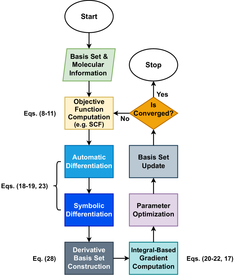
Figure 4: The diagram of the basis set optimization procedure. Within each optimization iteration cycle, both AD and SD are applied to parameter differentiation. Particularly, partial derivatives of basis functions with respect to basis set parameters are then transformed into a new derivative basis set $\mathbb{M}$ such that the cost of gradient computation can mostly rely on the direct electronic integral calculation in the teal box.

V Performance

To demonstrate the performance of Quiqbox (version 0.5.2 running on Julia 1.8.2), we compare it in three scenarios with existing packages that have limited similar features. The tests were run on a cluster node equipped with an Intel Xeon E7-8891 v4 CPU.

V.1 The Hartree--Fock method

As the Hartree--Fock method is currently the main objective function for basis set optimization in Quiqbox, it is crucial to verify the accuracy and efficiency of Quiqbox in performing such computations. We used the equal-spacing hydrogen chain, with the distance between adjacent nuclei being $1.0$ a.u., as a test system for how the computation accuracy and efficientcy scale with respect to the growth of system size. As for the package to benchmark against, we chose the widely-used ab initio electronic structure package PySCF (version 2.1.1 running on Python 3.9.12). The Hartree--Fock method, specifically RHF, was applied using each package with all the default settings except that the convergence threshold of RHF SCF iteration was manually set to be $1\!\times\!10^{-9}\,\rm{Ha}$. The multi-threading optimization was enabled for both packages, and the total number of available threads was set to 16. The benchmarking results are shown in FIG. 5. In FIG. 5(a), we show that with the hydrogen chain lengthening, Quiqbox can maintain better accuracy than PySCF, especially for smaller basis sets. Additionally, as shown in FIG. 5(a), Quiqbox, on average, needs less time to complete the SCF process than PySCF but has worse scaling. This is mainly due to the increasing relative inefficiency of Quiqbox’s electronic integral computation compared to PySCF.

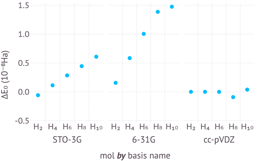
(a) The Hartree--Fock energies computed by PySCF minus the same quantities computed by Quiqbox.

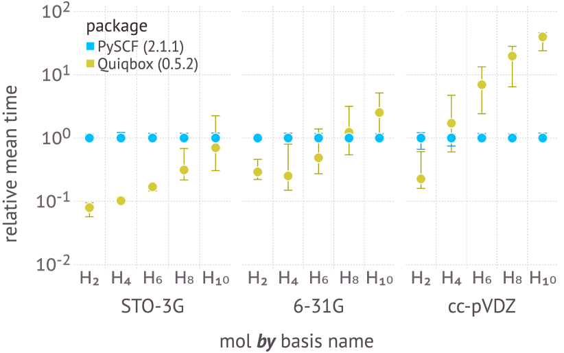
(b) The relative mean run time for Quiqbox’s Hartree--Fock SCF iteration with respect to PySCF. The upper error bar indicates the mean time plus one standard deviation, and the lower error bar records the minimal run time in each testing case.

Figure 5: The benchmark for Quiqbox’s RHF function against PySCF.

V.2 Electronic integrals

Instead of directly relying on an external Gaussian-type electronic integral library, we have written our own integral engine (also in Julia) as part of the core functions of Quiqbox, based on reference [50]. Additionally, we have added specialized optimization methods to avoid repetitive integral computation from the resulting tensor elements and the orbital expressions with shared parameters. On top of that, the integral engine is fully compatible with all kinds of MCGTOs. By contrast, PySCF relies on the C-based electronic integral library Libcint [62].

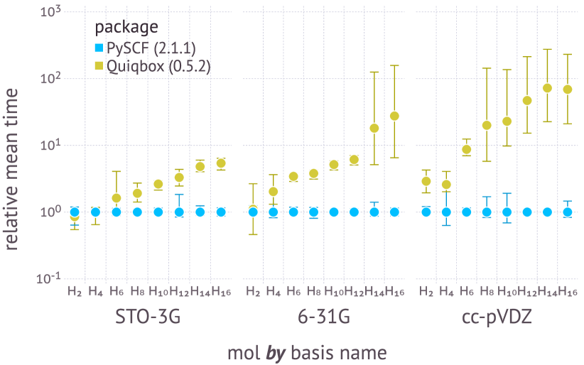
(a) The mean run time comparison of core Hamiltonian (one-electron tensor) computation.

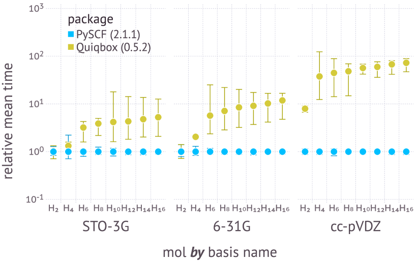
(b) The mean run time comparison of electron-electron interaction (two-electron tensor) computation.

Figure 6: The relative run time of electronic integral computation of Quiqbox’s native electronic integral engine with respect to Libcint used in PySCF. Same as in FIG. 5(b), the upper error bar indicates the mean time plus one standard deviation, and the lower error bar records the minimal run time in each testing case.

We compared the electronic integral computations between Quiqbox and Libcint for the same basis sets and molecules used in the Hartree--Fock tests. Quiqbox and Libcint agreed on all the computation results within a difference of $5\!\times\!10^{-7}$ a.u. In respect of computation efficiency, as shown in FIG. 6, for smaller basis sets such as STO-3G [34] and 6-31G [63], the minimal run time difference between Quiqbox’s integral engine and Libcint is within the same magnitude in best cases. For the cc-pVDZ [35] basis set (with optimized general contraction), the differences increase significantly, particularly for electron-electron interaction integrals. One possible reason is that Quiqbox’s integral engine does not take the spatial distribution of identical floating atomic orbitals (only $\bm{R}$ changes) into consideration to optimize the integral computation. For example, in an $\rm{H_{8}}$ chain, the integral computation of orbitals located at the 5th, 6th, 7th, and 8th hydrogen nuclei, should produce the same result as the integral computation of orbitals located at the 1st, 2nd, 3rd, 4th hydrogen nuclei after appropriate relabeling and reordering; thus they need not be recomputed. This type of issue can be avoided more easily by implementing more powerful integral computation reduction functions. Moreover, the author of Libcint has mentioned in their technical literature that they implemented hardware-level optimization such as CPU caching and addressing optimization in Libcint, as well as sparse matrix computation optimization on the software level [62], both of which are currently lacking in Quiqbox’s integral engine.

We believe that with more optimization in the future, we can improve Quiqbox’s integral engine to shorten the efficiency gap to Libcint. It is worth mentioning that implementing our native integral engine allows us to realize proper normalization for Cartesian-coordinate-based GTO integrals, which has been a legacy problem for Libcint [64], is crucial for realizing MCGTOs in Quiqbox.

V.3 Basis set parameter optimizations

To benchmark the performance of Quiqbox’s basis set optimization, we compared it with DiffiQult [16]. Since DiffiQult does not support basis sets beyond LACO, the selected basis set was the minimal basis set STO-3G [34] for both packages. Moreover, DiffiQult does not support multi-threading computation, so in the case of $\rm{H_{2}}$, Quiqbox is constrained to only use one thread both when running native Julia functions and when calling the default back-end linear algebra library OpenBLAS [65].

Nevertheless, Quiqbox’s optimization function shows a significant advantage against DiffiQult as presented in TABLE 1. Using the same numerical optimizer as DiffiQult, L-BFGS [66] with a line search algorithm using the strong Wolfe (SW) conditions, Quiqbox provided a 300 times speed-up. By replacing the line search algorithm with the one used in the nonlinear conjugate gradient method proposed by Hager and Zhang (HZ) [67], Quiqbox was able to achieve even faster convergence both in terms of the number of steps and overall computing time. This allowed a total of about 450 times speed-up relative to DiffiQult. When only using a first-order stochastic gradient descent optimizer like Adam [68], Quiqbox still outperformed DiffiQult with over 50 times speed-up. To be noted, we included two testing cases for $\rm{H_{2}}$: one was for optimizing only the exponent and contraction coefficients ($\alpha$ and $d$), and another one also added the GTO centers ($\bm{R}$). The reason for doing so is that DiffiQult does not support optimizing GTO centers while simultaneously optimizing the other two, which is not a limitation for Quiqbox.

The drastic improvement of basis set optimization’s efficiency pushes forward the practicality of variational basis set optimization, especially for larger systems. For example, in the case of optimizing the STO-3G basis set for LiH, Quiqbox was able to finish the optimization within two hours. In contrast, DiffiQult had not achieved convergence even after running for more than 11 hours. This result is included in TABLE 1 as well.

Molecule	Parameters		Package	Thread	Optimizer	$E_{0}$ (Ha)	Step	Time (sec)	Time/Step	Speed-up
	Types	Quantity
$\rm{H_{2}}$	$\alpha$, $d$	12	DiffiQult	1	L-BFGS (SW)	$-1.837307$	30	901.5	30.05	1.00
		12 (6)	Quiqbox	1	L-BFGS (SW)	$-1.837307$	34	3.0	0.09	300.50
					L-BFGS (HZ)	$-1.837307$	18	2.0	0.11	450.75
					Adam	$-1.837306$	489	12.4	0.03	72.70
	$\alpha$, $d$, $\bm{R}$	18	DiffiQult	1	L-BFGS (SW)	$-1.840628$	37	1122.9	30.35	1.00
		18 (9)	Quiqbox	1	L-BFGS (SW)	$-1.840820$	35	3.4	0.10	330.26
					L-BFGS (HZ)	$-1.840820$	21	3.1	0.15	362.22
					Adam	$-1.840782$	502	16.8	0.03	66.84
LiH	$\alpha$, $d$, $\bm{R}$	30	DiffiQult	1	L-BFGS (SW)	N/A	$>\!19$	$>\!4\!\times\!10^{4}$	N/A	1.00
		30 (28)	Quiqbox	1	L-BFGS (HZ)	$-8.963143$	433	6330.1	14.62	$>\!6.32$
			Quiqbox	8				5239.0	12.10	$>\!7.64$

Table 1: The benchmark for Quiqbox’s parameter optimization of STO-3G basis set concerning the RHF energy against DiffiQult. In the column ‘‘Parameters’’, $\alpha$, $d$, and $\bm{R}$ respectively represent all exponent coefficients, all contraction coefficients, and all orbital centers from the basis functions in the basis set. Each row of the sub-column ‘‘Quantity’’ shows the total number of parameters, with the extra number in parentheses (when they appear) being the reduced number of unique parameters to be optimized after imposing parameter correlations using Quiqbox’s basis set generation framework.

VI Example: building completely delocalized orbitals

Now we showcase the extra customizability Quiqbox provides. Consider a basis set $\{\phi^{\prime}_{n}\}$, where the Coulomb interaction between every two different spatial orbitals is equal to a constant $\mathcal{J}$, and the exchange-correlation between every two different spatial orbitals is equal to a constant $\mathcal{K}$, i.e.,

$$\forall\>\phi^{\prime}_{i},\>\phi^{\prime}_{j} \in\{\phi^{\prime}_{n}\}\>{\rm{s.t.}}\>\phi^{\prime}_{i}\neq\phi^{\prime}_{j},$$ (30)

$$\mathcal{J} \equiv(\phi^{\prime}_{i}\phi^{\prime}_{i}|\phi^{\prime}_{j}\phi^{\prime}_{j}),$$

$$\mathcal{K} \equiv(\phi^{\prime}_{i}\phi^{\prime}_{j}|\phi^{\prime}_{i}\phi^{\prime}_{j}).$$

Such basis sets can be defined as basis sets with ‘‘completely delocalized orbitals (CDOs)’’, resulting in permutation invariance of electronic modes with the same spin configuration.

One example of such a basis set is three pairs of identical floating CGTOs that all intersect at the same point such that every line segment that connects two CGTOs (at their centers) in the same pair is a perpendicular bisector of other pairs. The two CGTOs of each pair are combined as a new orbital in the basis set. If each CGTO contains $n$ GTOs, then in total, only $n$ floating GTOs with unique exponents and contraction coefficients are used to construct all three basis functions of the basis set.

The geometry of this basis set is shown in FIG. 7, and the code for constructing an instance of such type of basis set with $n\!=\!4$ (i.e., CDO3-4G) in Quiqbox is shown in line 10-36 of Listing 1.

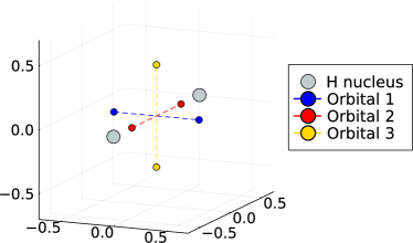
Figure 7: The geometry of a delocalized basis set of three orbitals (CDO3) concerning $\rm H_{2}$.

Listing 1: The Julia code of generating and optimizing a CDO3-4G basis set for $\rm{H_{2}}$ using Quiqbox.

⬇

1# Install Quiqbox if you haven't already

2using Pkg

3Pkg.add("Quiqbox")

4

5# Load Quiqbox

6using Quiqbox

7

8# The function to construct the center pairs

9# for delocalized orbitals

10function genDOcenters(l)

11 Lp = fill(l)|>Ref

12 shapes = [(1,0,0), (0,1,0), (0,0,1)]

13 GridBox.(shapes, Lp)

14end

15

16# The function to build a delocalized

17# orbital basis set

18function genDObs(l, gfs)

19 cPairs = genDOcenters(l)

20 map(cPairs) do cp

21 gp = gfs|>Ref

22 genBasisFunc.(cp.point, gp)|>sum

23 end

24end

25

26# Build an initial basis set

27gfs = [GaussFunc(17.0, 0.4),

28 GaussFunc( 2.5, 0.8),

29 GaussFunc( 0.5, 0.6),

30 GaussFunc( 0.1, 0.2)]

31bs = genDObs(1.5, gfs)

32

33# Extract the parameters to be optimized

34pp = markParams!(bs, true)|>Ref

35pSyms = [:L, :α, :d]

36pars = vcat(getParams.(pp, pSyms)...)

37

38# Specify the molecular geometry

39nuc = ["H", "H"]

40nucCoords = [[-0.7, 0.0, 0.0],

41 [ 0.7, 0.0, 0.0]]

42

43# Perform parameter optimization

44optimizeParams!(pars, bs,

45 nuc, nucCoords,

46 POconfig(maxStep=1000))

According to the fermionic de Finetti theorem [69], a fermionic quantum state of a finite-size system that is invariant under permutations of modes can be well described by a non-interacting fermionic state produced by mean-field methods. It would be of interest to study whether a CDO-based basis set that enforces the orbital permutation invariance would improve the performance of Hartree--Fock methods without losing much information from discretizing the molecular electronic Hamiltonian. Hence, we can use Quiqbox to perform parameter optimization of CDO3-4G (see lines 39--46 of Listing 1). The result of this optimization is compared to typical AOs in TABLE 2. CDO3-4G is able to produce lower Hartree--Fock energy for $\rm{H_{2}}$ with one-sixth as many orbitals as cc-pVDZ. This suggests the potential of using CDO-based basis sets to compress the information of the true ground state to a single Slater determinant state, as opposed to traditional AOs.

Basis set	$W$	$N_{\rm{GTO}}$	$E_{0}\>({\rm{Ha}})$	$E_{0}$ w.r.t. cc-pVDZ
STO-3G	$2$	$6$	$-1.83100$	$+0.651\%$
6-31G	$4$	$6$	$-1.84103$	$+0.107\%$
cc-pVDZ	$18$	$24$	$-1.84300$	$0.000\%$
CDO3-4G	$3$	$24$	$-1.84617$	$-0.172\%$
CDO3-nG	$3$	$\geq\!30$	$-1.84700$	$-0.217\%$

Table 2: The Hartree--Fock ground state energy approximations of ${\rm{H_{2}}}$ (with the bond length set to $1.4\;{\rm{a.u.}}$) using different basis sets. $N_{\rm{GTO}}$ represents the total number of GTO used for each basis set regardless of whether they share the same parameters. The CDO3 basis sets are optimized by Quiqbox to provide the lowest possible $E_{0}$. CDO3-nG is the asymptotic limit of the optimized CDO3 basis sets as the number of unique floating GTOs keeps increasing until $E_{0}$ converges.

As we see through this example, with Quiqbox, one can quickly construct and optimize a customized basis set to meet specific research needs. In other words, Quiqbox aims to be a ‘‘quick toolbox’’ for basis set study.

VII Conclusion and perspective

On the one hand, the ideas about Gaussian basis set design and optimization [36, 43, 70, 51, 52, 53] have been developing along the advance of classical ab initio calculation for electronic structure problems. On the other hand, the existing basis sets do not provide a smooth transition for NISQ devices to solve electronic structure problems practically. Nor do they permit proper benchmarks of VQE against existing classical algorithms. Tailoring new basis sets for specific scenarios becomes more in demand.

Aside from the need for a more customizable basis set design, we explained the significance of a more systematic study of basis sets beyond providing optimal numerical results for specific many-electron systems in Sec. II. Customizing and modifying basis sets to a higher degree across different systems will provide finer control of the electronic structure problem as a general computational problem and help study the effect of basis set discretization of electronic Hamiltonians.

To meet the abovementioned requirements, we proposed a highly customizable Gaussian-based basis set generation framework. It contains two main parts: basis set generation and parameter optimization. We introduced in Sec. III a type of more generalized Gaussian-based orbital named ‘‘mixed-contracted Gaussian-type orbital (MCGTO)’’ such that constructing basis sets beyond AOs using GTOs becomes possible. In Sec. IV, we then introduced a variational parameter optimization procedure for the basis sets composed of MCGTOs, which can be implemented with general electronic structure algorithms.

Moreover, this framework is already realized by the open-source software package, Quiqbox.jl, which we have developed using the high-performance dynamic programming language Julia [20, 21]. In Sec. V, we compared the performance of Quiqbox against other existing electronic structure packages. The results showcase Quiqbox’s capability and efficiency of variational basis set optimization and provide helpful feedback regarding Quiqbox’s potential improvement. Last but not least, we demonstrated using Quiqbox to construct basis sets of completely delocalized orbitals (CDOs). A CDO3-4G basis set consisting of three orbitals built from four unique floating GTOs can provide $0.2\%$ improvement for computing the Hartree--Fock energy of $\rm{H_{2}}$ compared to cc-pVDZ basis set with 18 orbitals (see TABLE 2).

In the future, we would like to add more post-Hartree--Fock methods as the objective functions for the basis set optimization. Doing so will have multiple benefits. First, it will help optimize and tailor the basis set for more electronic structure algorithms. Secondly, we can start studying the correlation between basis set geometry (through basis function designs and parameters) and the performance of corresponding algorithms. For instance, given a ground state ansatz, can one design a basis set that provides low-error discretization of the electronic Hamiltonian and reduces the computational cost of finding the ground state? If such a basis set exists, then the parameter space characterized by the basis set will contain a global minimum closer to the true ground-state wavefunction and allows the optimizer to find it easily. Additionally, we can incorporate the basis set completeness optimization technique into the basis set construction and parameter optimization [70, 71, 72], as it can help develop better automatic basis set generation procedures.

Finally, we would like to optimize Quiqbox’s performance further. Notably, we want to improve Quiqbox’s integral engine’s efficiency. In this way, besides being a basis set generation and optimization packages, it can also be a strong option for doing ab initio electronic structure computation in quantum chemistry and quantum physics.

VIII Acknowledgements

This paper was supported by the ‘‘Quantum Chemistry for Quantum Computers’’ project sponsored by the U.S. Department of Energy under Award No. DESC0019374. The authors are thankful for Brent Harrison’s proofreading and comments. JDW was supported by the US NSF grant PHYS-1820747 and NSF EPSCoR-1921199 and by the Office of Science, Office of Advanced Scientific Computing Research under programs Fundamental Algorithmic Research for Quantum Computing (FAR-QC) and the Optimization, Verification, and Engineered Reliability of Quantum Computers (OVER-QC) projects. JDW holds concurrent appointments at Dartmouth College and as an Amazon Visiting Academic. This paper describes work performed at Dartmouth College and is not associated with Amazon. WW would like to express his gratitude to his mother, father, and older sister. This paper would not have been possible without their utmost support. He would also like to thank his friends for their constant encouragement.

IX Appendix: Electronic Structure Acronyms and Notations

Acronym	Full name
AO	Atomic orbital.
GTO	Gaussian-type orbital.
CGTO	Contracted GTO.
LCAO	Linear combination of AOs.
MCGTO	Mixed-contracted GTO.

Table 3: The acronyms of all the single-particle spatial wavefunctions mentioned in the paper.

Symbol	Meaning
$N$	Number of electrons.
$N^{\uparrow}$	Number of spin-up electrons.
$N^{\downarrow}$	Number of spin-down electrons.
$N^{\prime}$	Number of nuclei.
$\mathbb{M}$	Set of nuclear positions and the corresponding charges.
$H_{elec}$	Electronic Hamiltonian.
$H_{nuc}$	Sum of nuclear kinetic and nuclear-nuclear repulsion energy.
$H_{tot}$	Total Hamiltonian.
$\mathcal{E}$	True ground state energy of $H_{elec}$.

Table 4: The notation convention in the paper of the physical variables determined by a many-electron system.

Symbol	Meaning
$\phi_{n}$	The $n$th basis function.
$\bm{S}$	The overlap matrix of basis set $\{\phi_{n}\,|\,n\!=\!1,\dots,W\}$.
$\varphi_{m}$	The $m$th orthonormalized basis function.
$\Psi_{0}$	Trial wavefunction of the approximate ground state based on an ansatz.
$\Phi_{n}$	The $n+1$th eigenfunction of the electronic Hamiltonian.
$\bm{c}$	Ansatz parameters of $\Psi_{0}$.
$\tilde{E_{0}}$	Energy expectation with respect to $\Psi_{0}$.
$E_{0}$	Lower bound of $\tilde{E_{0}}$.
$\bm{A}$	One-electron integral tensor with respect to $\{\varphi_{m}\}$.
$\bm{B}$	Two-electron integral tensor with respect to $\{\varphi_{m}\}$.
$\bm{c^{0}}$	Value of $\bm{c}$ that minimizes $\tilde{E_{0}}$ to $E_{0}$.
$\alpha$	The exponent coefficient of a GTO.
$\mathpzc{l}\!\equiv\!\mathpzc{i}\!+\!\mathpzc{j}\!+\!\mathpzc{k}$	The orbital angular momentum of a GTO.
$\bm{R}\!\equiv\![X,\,Y,\,Z]$	The center position of a GTO.
$d$	The contraction coefficient in a CGTO.
$\bm{\theta}\>\;(\{\theta_{i}\})$	Basis set parameters.
$\{p_{j}^{n}\}$	All the CGTO parameters of the $n$th basis function.
$\{p_{j}\}$	All the CGTO parameters in the basis set.
$\psi_{n}^{\theta_{i}}$	The basis function equivalent to the partial derivative of $\phi_{n}$ with respect to $\theta_{i}$.
$\mathbb{D}$	The derivative basis set that transforms the parameter gradients of elements in $\{\phi_{n}\}$ into its electronic integrals.

Table 5: The notations of the variables and quantities related to the basis functions defined in the paper.

References

- [1] Attila Szabo and Neil S Ostlund. Modern quantum chemistry: introduction to advanced electronic structure theory. Courier Corporation, 2012.
- [2] Juan Miguel Arrazola, Soran Jahangiri, Alain Delgado, Jack Ceroni, Josh Izaac, Antal Száva, Utkarsh Azad, Robert A Lang, Zeyue Niu, Olivia Di Matteo, et al. Differentiable quantum computational chemistry with pennylane. arXiv preprint arXiv:2111.09967, 2021.
- [3] John C Slater. A simplification of the hartree-fock method. Physical review, 81(3):385, 1951.
- [4] JG Valatin. Generalized hartree-fock method. Physical Review, 122(4):1012, 1961.
- [5] Rodney J Bartlett, Stanislaw A Kucharski, and Jozef Noga. Alternative coupled-cluster ansätze ii. the unitary coupled-cluster method. Chemical physics letters, 155(1):133--140, 1989.
- [6] Peter G Szalay, Thomas Muller, Gergely Gidofalvi, Hans Lischka, and Ron Shepard. Multiconfiguration self-consistent field and multireference configuration interaction methods and applications. Chemical reviews, 112(1):108--181, 2012.
- [7] Sam McArdle, Suguru Endo, Alán Aspuru-Guzik, Simon C Benjamin, and Xiao Yuan. Quantum computational chemistry. Reviews of Modern Physics, 92(1):015003, 2020.
- [8] Alberto Peruzzo, Jarrod McClean, Peter Shadbolt, Man-Hong Yung, Xiao-Qi Zhou, Peter J Love, Alán Aspuru-Guzik, and Jeremy L O’brien. A variational eigenvalue solver on a photonic quantum processor. Nature communications, 5(1):1--7, 2014.
- [9] John Preskill. Quantum computing in the nisq era and beyond. Quantum, 2:79, 2018.
- [10] Frank Leymann and Johanna Barzen. The bitter truth about gate-based quantum algorithms in the nisq era. Quantum Science and Technology, 5(4):044007, 2020.
- [11] Jarrod R McClean, Jonathan Romero, Ryan Babbush, and Alán Aspuru-Guzik. The theory of variational hybrid quantum-classical algorithms. New Journal of Physics, 18(2):023023, 2016.
- [12] Abhinav Kandala, Antonio Mezzacapo, Kristan Temme, Maika Takita, Markus Brink, Jerry M Chow, and Jay M Gambetta. Hardware-efficient variational quantum eigensolver for small molecules and quantum magnets. Nature, 549(7671):242--246, 2017.
- [13] Marco Cerezo, Andrew Arrasmith, Ryan Babbush, Simon C Benjamin, Suguru Endo, Keisuke Fujii, Jarrod R McClean, Kosuke Mitarai, Xiao Yuan, Lukasz Cincio, et al. Variational quantum algorithms. Nature Reviews Physics, 3(9):625--644, 2021.
- [14] Jules Tilly, Hongxiang Chen, Shuxiang Cao, Dario Picozzi, Kanav Setia, Ying Li, Edward Grant, Leonard Wossnig, Ivan Rungger, George H Booth, et al. The variational quantum eigensolver: a review of methods and best practices. Physics Reports, 986:1--128, 2022.
- [15] Susi Lehtola. Automatic algorithms for completeness-optimization of g aussian basis sets, 2015.
- [16] Teresa Tamayo-Mendoza, Christoph Kreisbeck, Roland Lindh, and Alán Aspuru-Guzik. Automatic differentiation in quantum chemistry with applications to fully variational hartree--fock. ACS central science, 4(5):559--566, 2018.
- [17] Muhammad F Kasim, Susi Lehtola, and Sam M Vinko. Dqc: A python program package for differentiable quantum chemistry. The Journal of chemical physics, 156(8):084801, 2022.
- [18] Andreas Griewank et al. On automatic differentiation. Mathematical Programming: recent developments and applications, 6(6):83--107, 1989.
- [19] Atilim Gunes Baydin, Barak A Pearlmutter, Alexey Andreyevich Radul, and Jeffrey Mark Siskind. Automatic differentiation in machine learning: a survey. Journal of Marchine Learning Research, 18:1--43, 2018.
- [20] Jeff Bezanson, Stefan Karpinski, Viral B Shah, and Alan Edelman. Julia: A fast dynamic language for technical computing. arXiv preprint arXiv:1209.5145, 2012.
- [21] Jeff Bezanson, Jiahao Chen, Benjamin Chung, Stefan Karpinski, Viral B Shah, Jan Vitek, and Lionel Zoubritzky. Julia: Dynamism and performance reconciled by design. Proceedings of the ACM on Programming Languages, 2(OOPSLA):1--23, 2018.
- [22] Weishi Wang. Quiqbox.jl. The code repository of the package: https://github.com/frankwswang/Quiqbox.jl.
- [23] Andrew J Daley, Immanuel Bloch, Christian Kokail, Stuart Flannigan, Natalie Pearson, Matthias Troyer, and Peter Zoller. Practical quantum advantage in quantum simulation. Nature, 607(7920):667--676, 2022.
- [24] James D Whitfield, Jun Yan, Weishi Wang, Joshuah T Heath, and Brent Harrison. Quantum computing 2022. arXiv preprint arXiv:2201.09877, 2022.
- [25] Peter Pulay. Improved scf convergence acceleration. Journal of Computational Chemistry, 3(4):556--560, 1982.
- [26] Konstantin N Kudin, Gustavo E Scuseria, and Eric Cances. A black-box self-consistent field convergence algorithm: One step closer. The Journal of chemical physics, 116(19):8255--8261, 2002.
- [27] Xiangqian Hu and Weitao Yang. Accelerating self-consistent field convergence with the augmented roothaan--hall energy function. The Journal of chemical physics, 132(5):054109, 2010.
- [28] Naruki Yoshikawa and Masato Sumita. Automatic differentiation for the direct scf approach to the hartree-fock method. arXiv preprint arXiv:2203.04441, 2022.
- [29] Bryan O’Gorman, Sandy Irani, James Whitfield, and Bill Fefferman. Intractability of electronic structure in a fixed basis. PRX Quantum, 3(2):020322, 2022.
- [30] Sergey B Bravyi and Alexei Yu Kitaev. Fermionic quantum computation. Annals of Physics, 298(1):210--226, 2002.
- [31] Vojtěch Havlíček, Matthias Troyer, and James D Whitfield. Operator locality in the quantum simulation of fermionic models. Physical Review A, 95(3):032332, 2017.
- [32] Kanav Setia, Sergey Bravyi, Antonio Mezzacapo, and James D Whitfield. Superfast encodings for fermionic quantum simulation. Physical Review Research, 1(3):033033, 2019.
- [33] Alán Aspuru-Guzik, Anthony D Dutoi, Peter J Love, and Martin Head-Gordon. Simulated quantum computation of molecular energies. Science, 309(5741):1704--1707, 2005.
- [34] Robert F Stewart. Small gaussian expansions of slater-type orbitals. The Journal of Chemical Physics, 52(1):431--438, 1970.
- [35] Thom H Dunning Jr. Gaussian basis sets for use in correlated molecular calculations. i. the atoms boron through neon and hydrogen. The Journal of chemical physics, 90(2):1007--1023, 1989.
- [36] Masanori Tachikawa, Kento Taneda, and Kazuhide Mori. Simultaneous optimization of gtf exponents and their centers with fully variational treatment of hartree--fock molecular orbital calculation. International journal of quantum chemistry, 75(4-5):497--510, 1999.
- [37] Adam D Bookatz. Qma-complete problems. arXiv preprint arXiv:1212.6312, 2012.
- [38] Yuri Manin. Computable and uncomputable. Sovetskoye Radio, Moscow, 128, 1980.
- [39] Richard P Feynman. Simulating physics with computers. In Feynman and computation, pages 133--153. CRC Press, 2018.
- [40] Benjamin P Lanyon, James D Whitfield, Geoff G Gillett, Michael E Goggin, Marcelo P Almeida, Ivan Kassal, Jacob D Biamonte, Masoud Mohseni, Ben J Powell, Marco Barbieri, et al. Towards quantum chemistry on a quantum computer. Nature chemistry, 2(2):106--111, 2010.
- [41] Marco Cerezo, Andrew Arrasmith, Ryan Babbush, Simon C Benjamin, Suguru Endo, Keisuke Fujii, Jarrod R McClean, Kosuke Mitarai, Xiao Yuan, Lukasz Cincio, et al. Variational quantum algorithms. Nature Reviews Physics, 3(9):625--644, 2021.
- [42] Georg Kresse and Jürgen Furthmüller. Efficient iterative schemes for ab initio total-energy calculations using a plane-wave basis set. Physical review B, 54(16):11169, 1996.
- [43] Georg Kresse and Jürgen Furthmüller. Efficiency of ab-initio total energy calculations for metals and semiconductors using a plane-wave basis set. Computational materials science, 6(1):15--50, 1996.
- [44] JE Pask, BM Klein, CY Fong, and PA Sterne. Real-space local polynomial basis for solid-state electronic-structure calculations: A finite-element approach. Physical Review B, 59(19):12352, 1999.
- [45] Luigi Genovese, Alexey Neelov, Stefan Goedecker, Thierry Deutsch, Seyed Alireza Ghasemi, Alexander Willand, Damien Caliste, Oded Zilberberg, Mark Rayson, Anders Bergman, et al. Daubechies wavelets as a basis set for density functional pseudopotential calculations. The Journal of chemical physics, 129(1):014109, 2008.
- [46] Laura E Ratcliff, William Dawson, Giuseppe Fisicaro, Damien Caliste, Stephan Mohr, Augustin Degomme, Brice Videau, Viviana Cristiglio, Martina Stella, Marco D’Alessandro, et al. Flexibilities of wavelets as a computational basis set for large-scale electronic structure calculations. The Journal of chemical physics, 152(19):194110, 2020.
- [47] Thom Dunning, P Jeffrey Hay, et al. Gaussian basis sets for molecular calculations. In Methods of electronic structure theory, pages 1--27. Springer, 1977.
- [48] J Grant Hill. Gaussian basis sets for molecular applications. International Journal of Quantum Chemistry, 113(1):21--34, 2013.
- [49] Martin Head-Gordon and John A Pople. A method for two-electron gaussian integral and integral derivative evaluation using recurrence relations. The Journal of chemical physics, 89(9):5777--5786, 1988.
- [50] Tomas Petersson and Bo Hellsing. A detailed derivation of gaussian orbital-based matrix elements in electron structure calculations. European journal of physics, 31(1):37, 2009.
- [51] AC Hurley. The computation of floating functions and their use in force constant calculations. Journal of computational chemistry, 9(1):75--79, 1988.
- [52] Arthur A Frost. Floating spherical gaussian orbital model of molecular structure. i. computational procedure. lih as an example. The Journal of Chemical Physics, 47(10):3707--3713, 1967.
- [53] Hanspeter Huber. Geometry optimization in ab initio calculations. floating orbital geometry optimization applying the hellmann-feyman force. Chemical Physics Letters, 62(1):95--99, 1979.
- [54] Steven R White. Hybrid grid/basis set discretizations of the schrödinger equation. The Journal of chemical physics, 147(24):244102, 2017.
- [55] Steven R White and E Miles Stoudenmire. Multisliced gausslet basis sets for electronic structure. Physical Review B, 99(8):081110, 2019.
- [56] Ira Cherkes, Shachar Klaiman, and Nimrod Moiseyev. Spanning the hilbert space with an even tempered gaussian basis set. International Journal of Quantum Chemistry, 109(13):2996--3002, 2009.
- [57] Qiming Sun, Xing Zhang, Samragni Banerjee, Peng Bao, Marc Barbry, Nick S Blunt, Nikolay A Bogdanov, George H Booth, Jia Chen, Zhi-Hao Cui, et al. Recent developments in the pyscf program package. The Journal of chemical physics, 153(2):024109, 2020.
- [58] Daniel GA Smith, Lori A Burns, Andrew C Simmonett, Robert M Parrish, Matthew C Schieber, Raimondas Galvelis, Peter Kraus, Holger Kruse, Roberto Di Remigio, Asem Alenaizan, et al. Psi4 1.4: Open-source software for high-throughput quantum chemistry. The Journal of chemical physics, 152(18):184108, 2020.
- [59] David M Bishop. Group theory and chemistry. Courier Corporation, 1993.
- [60] Poul Jørgensen and Jack Simons. Ab initio analytical molecular gradients and hessians. The Journal of Chemical Physics, 79(1):334--357, 1983.
- [61] Peter Politzer and Jane S Murray. The hellmann-feynman theorem: a perspective. Journal of molecular modeling, 24(9):1--7, 2018.
- [62] Qiming Sun. Libcint: An efficient general integral library for gaussian basis functions. Journal of Computational Chemistry, 36:1664--1671, 2015.
- [63] Warren J Hehre, Robert Ditchfield, and John A Pople. Self—consistent molecular orbital methods. xii. further extensions of gaussian—type basis sets for use in molecular orbital studies of organic molecules. The Journal of Chemical Physics, 56(5):2257--2261, 1972.
- [64] libcint github issue: How to rescale coefficients, 2017.
- [65] Qian Wang, Xianyi Zhang, Yunquan Zhang, and Qing Yi. Augem: automatically generate high performance dense linear algebra kernels on x86 cpus. In SC’13: Proceedings of the International Conference on High Performance Computing, Networking, Storage and Analysis, pages 1--12. IEEE, 2013.
- [66] Dong C Liu and Jorge Nocedal. On the limited memory bfgs method for large scale optimization. Mathematical programming, 45(1):503--528, 1989.
- [67] William W Hager and Hongchao Zhang. A new conjugate gradient method with guaranteed descent and an efficient line search. SIAM Journal on optimization, 16(1):170--192, 2005.
- [68] Diederik P Kingma and Jimmy Ba. Adam: A method for stochastic optimization. arXiv preprint arXiv:1412.6980, 2014.
- [69] Christian Krumnow, Zoltán Zimborás, and Jens Eisert. A fermionic de finetti theorem. Journal of Mathematical Physics, 58(12):122204, 2017.
- [70] Donald G Truhlar. Basis-set extrapolation. Chemical Physics Letters, 294(1-3):45--48, 1998.
- [71] Pekka Manninen and Juha Vaara. Systematic gaussian basis-set limit using completeness-optimized primitive sets. a case for magnetic properties. Journal of computational chemistry, 27(4):434--445, 2006.
- [72] Susi Lehtola. Automatic algorithms for completeness-optimization of gaussian basis sets. Journal of Computational Chemistry, 36(5):335–347, 2014.