A Double Regression Method for Graphical Modeling of High-dimensional Nonlinear and Non-Gaussian Data

Abstract

Graphical models have long been studied in statistics as a tool for inferring conditional independence relationships among a large set of random variables. The most existing works in graphical modeling focus on the cases that the data are Gaussian or mixed and the variables are linearly dependent. In this paper, we propose a double regression method for learning graphical models under the high-dimensional nonlinear and non-Gaussian setting, and prove that the proposed method is consistent under mild conditions. The proposed method works by performing a series of nonparametric conditional independence tests. The conditioning set of each test is reduced via a double regression procedure where a model-free sure independence screening procedure or a sparse deep neural network can be employed. The numerical results indicate that the proposed method works well for high-dimensional nonlinear and non-Gaussian data.

Keywords: Conditional Independence Tests, Directed Acyclic Graph, Dimension Reduction, Markov Blanket, Markov Network.

1 Introduction

Graphical models, which generally refer to undirected Markov networks, have proven to be a useful tool for inferring conditional independence relationships for a large set of random variables. They are particularly useful under the high-dimensional scenario, i.e., when the number of random variables is greater than the number of observations. In this scenario, with the aid of the sparse graphical model learned for the explanatory variables, the inference for high-dimensional regression is reduced to the inference for a series of low-dimensional regression, for which the $t$-test can be used for inference of the significance and associated confidence interval for each explanatory variable. See Liang et al. (2021) for the details. As an alternative to undirected Markov networks, Bayesian networks can also serve the purpose of inference for the conditional independence relationships for a large set of random variables. However, Bayesian networks are directed and focus more on data generating mechanisms. It is worth noting that the Bayesian network can be constructed from its moral graph, which is an undirected Markov network, using a collider set algorithm (Pellet and Elisseeff, 2008) or local neighborhood algorithm (Margaritis and Thrun, 2000) to have the edge directions added. Therefore, learning undirected Markov networks is fundamental, which is the focus of this paper.

In practice, the random variables can be Gaussian or non-Gaussian, and the dependence between different random variables can be linear or nonlinear. However, most of the existing works in graphical modeling focus on Gaussian data with linear dependence. Under the Gaussian and linear assumptions, various methods have been developed based on the properties of partial correlation coefficients, concentration matrix, and regression coefficients of Gaussian graphical models (GGMs), see e.g., graphical Lasso (Yuan and Lin, 2007; Friedman et al., 2008), nodewise regression (Meinshausen and Bühlmann, 2006), $\psi$-learning (Liang et al., 2015), and structural equation modeling (Zheng et al., 2018). To be more detailed, let $\{X_{1},X_{2},\ldots,X_{p}\}$ denote a set of zero-mean Gaussian random variables, let $V=\{1,2,\ldots,p\}$ denote its index set, let $\Sigma$ denote the covariance matrix of the random variables, let $C=\Sigma^{-1}$ denote the concentration matrix, and let $\beta_{i}^{(j)}$ denote a coefficient of the normal linear regression

$$X_{j}=\beta_{i}^{(j)}X_{i}+\sum_{r\in V\setminus\{i,j\}}\beta_{r}^{(j)}X_{r}+\epsilon_{j},\quad j=1,2,\ldots,p,$$ (1)

where $\epsilon_{j}$ is a zero-mean Gaussian random error. By the standard theory on normal linear regression, see e.g. chapter 13 of Bühlmann and van de Gerer (2011), the following relation holds:

$$\rho_{ij|V\setminus\{i,j\}}\neq 0\Longleftrightarrow C_{ij}\neq 0\Longleftrightarrow\beta_{i}^{(j)}\neq 0,$$ (2)

where $\rho_{ij|V\setminus\{i,j\}}$ denotes the partial correlation coefficient of $X_{i}$ and $X_{j}$ conditioned on all other variables, and $C_{ij}$ denotes the $(i,j)$th element of the concentration matrix $C$. Based on this relation, the graphical Lasso method (Yuan and Lin, 2007; Friedman et al., 2008) infers the GGM by directly estimating the concentration matrix via a regularization approach; the nodewise regression method (Meinshausen and Bühlmann, 2006) infers the GGM by computing the coefficient $\beta_{i}^{(j)}$ for each pair of variables $(X_{j},X_{i})$ via a regularized regression; the graphical regression method (Ni et al., 2019; Zhang and Li, 2020) regresses both the mean and the precision matrix of a GGM on covariates, which enables estimation of subject-specific graphical models; the $\psi$-learning method (Liang et al., 2015) infers the GGM by an equivalent measure of the partial correlation coefficient $\rho_{ij|V\setminus\{i,j\}}$, which can be computed based on a reduced conditioning set; and the structural equation modeling method (Zheng et al., 2018) infers a directed acyclic graph (DAG) for the GGM by directly solving the structure equations formed by the nodewise regression (1), where the problem was formulated as a continuous optimization problem with a structural constraint (Harary and Manvel, 1971) for ensuring acyclicity of the graph.

Many authors have tried to extend the methods developed for GGMs to non-Gaussian data or mixed data under the assumption that the random variables are still linearly dependent. For example, Ravikumar et al. (2010) extends the nodewise regression method to binary data; Lee and Hastie (2013), Cheng et al. (2013) and Yang et al. (2014) extends the nodewise regression method to mixed data; Xu et al. (2019) extends the $\psi$-learning method to mixed data; and Fan et al. (2017) extends the graphical Lasso method to mixed data by introducing some latent variables for the observed discrete variables. However, as pointed out in Fan et al. (2017), the latent variable method does not necessarily lead to correct graphical models, as the conditional independence relationship between the latent variables does not imply the conditional independence relationship between the observed discrete variables. The copula PC method (Cui et al., 2016) suffers from the same issue. Quite recently, Zheng et al. (2020) extends the structural equation modeling method to certain types of nonlinear models defined in the Sobolev space. However, it is unclear whether the method can lead to consistent estimation of the underlying graphical models under the high-dimensional scenario. Some other methods, e.g. Yu et al. (2019), infer the model in an approximate sense using variational autoencoder, and it is unclear whether it can lead to the conditional independence relationships pursued in graphical modeling.

Up to our knowledge, none of the works has been done for inference of graphical models under the general high-dimensional nonlinear and non-Gaussian setting. To tackle this problem, we proposed a double regression method. The proposed method works by performing a series of nonparametric conditional independence tests, for each of which the conditioning set is reduced by a double regression procedure. The proposed method is shown to be consistent under mild conditions. The numerical results indicate that the proposed method works well for high-dimensional nonlinear and non-Gaussian data.

Statistical learning for nonlinear and non-Gaussian models is important, as in modern data science nonlinear dependency is common and the data may not tend towards Gaussian distributions, such as biological data and financial data. Researchers have found that although the accuracy of the partial correlation test-based GGM methods are not significantly affected by violations of the Gaussian assumption, they are significantly affected by violations of the linear dependency assumption, see e.g. Voortman and Druzdzel (2008) for more discussions on this issue. Researchers have also found that nonlinearity and non-Gaussianity can actually be a blessing, and nonlinear non-Gaussian modeling can reveal more accurate information about the true data generating process than the linear and Gaussian approximation. For example, Shimizu et al. (2006) and Hoyer et al. (2008) found that non-Gaussianity is helpful in predicting causal relationships among the variables.

The remaining part of this article is organized as follows. Section 2 describes the proposed method and establishes its consistency. Section 3 illustrates the proposed method using simulated data. Section 4 applies the proposed method to identification of drug-sensitive genes with the cancer cell line encyclopedia (CCLE) data. Section 5 analyzes the computational complexity of the proposed method. Section 6 concludes the paper with a brief discussion.

2 Double Regression Method

2.1 The Algorithm

Notations: Consider a set of random variables $\{X_{1},X_{2},\ldots,X_{p}\}$, where each variable can be non-Gaussian and the dependence between different variables can be nonlinear. The dimension $p$ is assumed to grow with the sample size $n$. To indicate this dependence, we rewrite $p$ as $p_{n}$ in what follows. Let $V=\{1,2,\ldots,p_{n}\}$ be the index set of the variables, let $A\subset V$ be a subset of $V$, and let ${\bm{X}}_{A}=\{X_{k}:k\in A\}$.

As our goal is to construct a graphical model for the variables, the conditional independence test (CIT) $X_{i}\rotatebox[origin={c}]{90.0}{$\models$}X_{j}|X_{V\setminus\{i,j\}}$ needs to be conducted for each pair of the variables $(X_{i},X_{j})$. Since the functional form of the dependence between different variables is unknown, a nonparametric CIT can be applied here. An abundance of nonparametric CITs have been developed in the literature. A non-exhaustive list includes permutation-based tests (Doran et al., 2014a; Berrett et al., 2019), kernel-based tests (Zhang et al., 2012a; Strobl et al., 2019), classification or regression-based tests (Sen et al., 2017; Zhang et al., 2017), knockoff-based tests (Candès et al., 2018), and generative adversarial network (GAN)-based tests (Bellot and van der Schaar, 2019a). Refer to Li and Fan (2019) for a comprehensive overview.

As pointed out in Li and Fan (2019), the existing nonparametric CITs often suffer from the curse of dimensionality in the confounding set; that is, the tests may be ineffective when the sample size is small, since the accumulation of spurious correlations from a large number of confounding variables makes them difficult to discriminate between the hypotheses. To tackle this issue, we consider the following simple mathematical fact of conditional probability distributions:

$$\begin{split}P(X_{i},X_{j}|{\bm{X}}_{V\setminus\{i,j\}})&=P(X_{i}|X_{j},{\bm{X}}_{V\setminus\{i,j\}})P(X_{j}|{\bm{X}}_{V\setminus\{i,j\}})=P(X_{i}|X_{j},{\bm{X}}_{S_{i}\setminus\{j\}})P(X_{j}|{\bm{X}}_{S_{j\setminus i}})\\ &=P(X_{i},X_{j}|{\bm{X}}_{S_{i}\setminus\{j\}},{\bm{X}}_{S_{j\setminus i}})=P(X_{i},X_{j}|{\bm{X}}_{S_{i}\cup S_{j\setminus i}\setminus\{j\}}),\end{split}$$ (3)

where ${\bm{X}}_{S_{i}}$ denotes the set of true variables of the nonlinear regression $X_{i}\sim{\bm{X}}_{V\setminus\{i\}}$, and ${\bm{X}}_{S_{j\setminus i}}$ denotes the set of true variables of the nonlinear regression $X_{j}\sim{\bm{X}}_{V\setminus\{i,j\}}$. Based on this property of conditional probability distributions, we propose the double regression method which is summarized in Algorithm 1 and can be used for reducing the conditioning sets of the CITs.

for each variable $X_{i}$, $i=1,2,\ldots,p_{n}$ do

       (i) Variable selection: conduct nonlinear/non-Gaussian regression

$$X_{i}\sim{\bm{X}}_{V\setminus\{i\}},$$ (4)

and select a subset of variables. Denote the index set of the selected variables by $\hat{S}_{i}$, which can be viewed as an estimate of $S_{i}$.

end for

for each pair of variables $(X_{i},X_{j})$, $1\leq j<i\leq p_{n}$ do

       (ii) Variable selection: conduct nonlinear/non-Gaussian regression

$$X_{j}\sim{\bm{X}}_{V\setminus\{i,j\}},$$ (5)

and select a subset of variables. Denote the index set of the selected variables by $\hat{S}_{j\setminus i}$, which can be viewed as an estimate of $S_{j\setminus i}$.

      (iii) Conditional independence test: perform nonparametric conditional independence test

$$X_{i}\rotatebox[origin={c}]{90.0}{$\models$}X_{j}|{\bm{X}}_{\hat{S}_{i}\cup\hat{S}_{j\setminus i}\setminus\{j\}},$$ (6)

and denote the $p$-value of the test by $q_{ij}$.

end for

(iv) Multiple hypothesis test: perform a multiple hypothesis test for all pairs of variables based on the $p$-values $\{q_{ij}:1\leq j<i\leq p_{n}\}$, and identify the pairs for which the $p$-values are significantly smaller than others.

Algorithm 1 Double Regression

The proposed method is called double regression, as for each conditional independence test two regression tasks need to be performed in order to reduce the size of the conditioning set. Regarding this method, we have three remarks:

Remark 1.

When $X_{i}$’s are Gaussian and linearly dependent, the double regression method is reduced to the $\psi$-learning method (Liang et al., 2015), for which it can be shown that the $p$-value of the conditional independence test (6) provides an equivalent measure for the partial correlation coefficient $\rho_{ij|V\setminus\{i,j\}}$ in determining the structure of the GGM. Note that, for GGMs, the conditioning set used in (6) can be further reduced based on the Markov and faithfulness properties as shown in Liang et al. (2015).

Remark 2.

In addition to consistent variable selection procedures, (3) also holds for variable sure screening procedures. In practice, variable screening for high-dimensional nonlinear regression can be done using Bayesian sparse neural networks (Liang et al., 2018; Sun et al., 2021), which are shown to have the sure screening property for both normal and multinomial logistic regression. For other continuous variables, a nonparanormal transformation (Liu et al., 2009) can be applied before the application of Bayesian sparse neural networks. One can also replace the Bayesian sparse neural network by a model-free sure independence screening (SIS) procedure, say, the Henze-Zirkler sure independence screening (HZ-SIS) procedure proposed by Xue and Liang (2017) for nonlinear regression with continuous variables, and the sure independence screening procedure proposed by Cui et al. (2015) for nonlinear regression with a categorical response variable. When a sure independence screening procedure is used, we recommend to select $n/(c\log(n))$ variables for each regression task, where $c$ may slightly vary from 1 for different problems. More interestingly, the above two types of variable screening procedures can be used in a combined manner; that is, one can first perform a SIS procedure to reduce the dimension of the conditioning set, and then perform Bayesian sparse neural networks to have the dimension of the reduced conditioning set reduced further.

Remark 3.

Our recommendations for the variable sure screening methods and nonparametric conditional independence tests (CIT) are summarized in Table 1.

Table 1: Methods recommended for variable sure screening and nonparametric conditional independence tests.

Procedure	Recommended Methods
Variable Sure Screening	Methods collected in Model-free SIS Procedures (Cheng et al., 2022), Henze-Zirkler SIS (Xue and Liang, 2017), Sparse BNN (Liang et al., 2018; Sun et al., 2021)
Nonparametric Conditional Independence Test (CIT)	Kernel CIT (Zhang et al., 2012b), Conditional Distance Independence Test (Wang et al., 2015), Permutation-based Kernel CIT (Doran et al., 2014b), Generative CIT (Bellot and van der Schaar, 2019b)

2.2 Consistency

This section establishes the consistency of the proposed double regression method for learning graphical models with high-dimensional nonlinear and/or non-Gaussian data. Let $T_{ij}$ denote the test statistic used in the conditional independence test (6). Let $\hat{\mathcal{E}}_{n}$ denote the resulting network by Algorithm 1. To study the consistency of $\hat{\mathcal{E}}_{n}$, we make the following assumptions.

Assumption 1.

(Markov and faithfulness properties) The generative distribution of the data is Markov and faithful to a directed acyclic graph.

Assumption 2.

(High dimensionality) The dimension $p_{n}$ increases in a polynomial of the sample size $n$.

Assumption 3.

(Uniform sure screening property) The variable screening procedure satisfies the uniform sure screening property, i.e., $\min_{1\leq i\leq p_{n}}P(S_{i}\subset\hat{S}_{i})\to 1$ and $\min_{1\leq j<i\leq p_{n}}P(S_{j\setminus i}\subset\hat{S}_{j\setminus i})\to 1$ hold as the sample size $n\to\infty$.

Assumption 4.

(Separation) $\min_{i,j}(\mu_{ij,1}-\mu_{ij,0})>\eta_{n}$, where $\eta_{n}=c_{0}n^{-\kappa}$ for some constant $c_{0}>0$ and $\kappa>0$, and $\mu_{ij,0}$ and $\mu_{ij,1}$ denote the mean values of the test statistic $T_{ij}$ under the null (conditionally independent) and alternative (conditionally dependent) hypotheses, respectively.

Assumption 5.

(Tail probability)

$$\sup_{i,j}P(|T_{ij}-\mu_{ij}|>\frac{1}{2}\eta_{n})=\exp\left\{-O(n^{\delta(\kappa)})\right\},$$

where $\mu_{ij}=E(T_{ij})$ denotes the expectation of $T_{ij}$, and $\delta(\kappa)$ is positive number depending on $\kappa$.

Regarding these assumptions, we have the following comments. Assumptions 1 and 2 are regular for high-dimensional graphical models. Similar assumptions have been used in the study of Gaussian graphical models, see e.g. Liang et al. (2015). Assumption 3 ensures asymptotic validity of the conditional independence tests on reduced conditioning sets. Under Assumption 2, it is easy to verify that the uniform sure screening property is satisfied by many existing sure independence screening procedures such as those proposed in Xue and Liang (2017) and Cui et al. (2015). This property also holds for Bayesian sparse neural networks under Assumption 2. Assumptions 4 and 5 are on the distribution of the test statistics. Assumptions 4 is like the $\beta$-min condition used in high-dimensional variable selection, see e.g. Dezeure et al. (2015) and Van de Geer et al. (2011). This condition basically requires that the gap between the mean values of the test statistics under the null and alternative hypotheses are “sufficiently large” to separate, which seems necessary for proving the consistency of Algorithm 1. Assumption 5 constrains the tail probability of the distribution. Without loss of generality, we can assume that $T_{ij}$ is an average-type test statistic and follows a sub-Gaussian distribution. Then, by the concentration inequality, it is easy to show that Assumption 5 holds provided that $0<\kappa<1/2$ and $0<\delta(\kappa)<1-2\kappa$.

Let $A_{ij}$ denote that an error event occurs when testing the hypotheses $H_{0}:e_{ij}=0$ versus $H_{1}:e_{ij}=1$, where $e_{ij}=0$ and $e_{ij}=1$ denote that the variables $X_{i}$ and $X_{j}$ are conditionally independent and dependent, respectively. Thus,

$$P\{\mbox{an error occurs in $\hat{\mathcal{E}}_{n}$}\}=P(\cup_{i>j}A_{ij})\leq O(p_{n}^{2})\sup_{i>j}P(A_{ij}).$$ (7)

Then based on the Assumption 1 - 5, we have the following theorem.

Theorem 1.

Suppose Assumptions 1-5 hold. For each pair of variables $(X_{i},X_{j})$, let $\mu_{ij,0}+\eta_{n}/2$ denote the critical value of the conditional independence test (6). Then the network estimate is consistent, i.e., $P\{\mbox{an error occurs in $\hat{\mathcal{E}}_{n}$}\}\to 0$ as $n\to\infty$.

Theorem 1 establishes consistency of the double regression method. In other words, it shows that if constructing the network with the double regression method, the probability of mistakenly adding or removing one edge converges to 0 as the sample size goes to infinity. The proof is presented in the Appendix.

3 Synthetic Examples

Example 1

We generated 100 datasets from the following nonlinear and non-Gaussian model

$$\begin{split}X_{1}&\sim Unif[-1,1],\\ X_{2}&=6\cos(X_{1})+\epsilon_{2},\quad\epsilon_{2}\sim Unif[-1,1],\\ X_{3}&=5\sin(X_{1})+X_{2}+\epsilon_{3},\quad\epsilon_{3}\sim N(0,1),\\ X_{4}&=5\cos(X_{3}X_{6})+3X_{3}+3X_{6}+\epsilon_{4},\quad\epsilon_{4}\sim N(0,1),\\ X_{5}&=0.05(X_{2}+X_{6})^{3}+\epsilon_{5},\quad\epsilon_{5}\sim N(0,1),\\ X_{6}&\sim Unif[-1,1],\\ X_{7}&=6\cos(0.2(X_{3}+\log(|5X_{5}|+1)))+\epsilon_{7},\quad\epsilon_{7}\sim Unif[-1,1],\\ X_{i}&\sim N(0,1),\quad i=8,9,\ldots,p_{n}.\\ \end{split}$$ (8)

In this example, we set the dimension $p_{n}=30$ and the sample size $n=400$. To goal of this example is to compare the proposed method with the existing methods, such as notears and DAG-GNN, under their ideal setting. Note that both the methods notears and DAG-GNN are developed under the low-dimensional scenario.

Algorithm 1 was applied to this example with HZ-SIS (Xue and Liang, 2017) used in variable screening and the randomized conditional correlation test (RCoT) (Strobl et al., 2019) used in nonparametric conditional independence test. The network edges in step (c) of Algorithm 1 are identified based on the adjusted $p$-values (Holm, 1979). We use the averaged Areas Under the precision-recall Curves (AUC) as the metric to evaluate the performance of different methods. Refer to Appendix A.2 for the definitions of precision and recall. The numerical results are summarized in Figure 1 and Table 2.

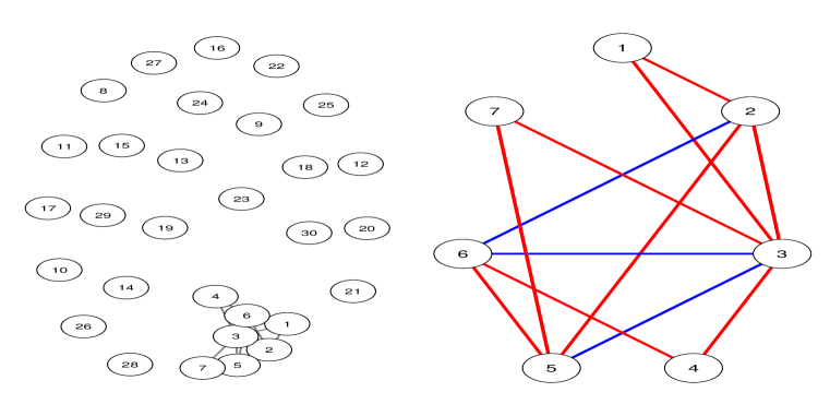
Figure 1: Markov networks identified by Algorithm 1 for one simulated dataset of the model (8) at a significance level of 0.01 based on adjusted $p$-values: (left plot) full network; (right plot) subnetwork of the nodes $X_{1}-X_{7}$, where the red lines indicate parents/children relationships and the blue lines indicate spouse relationships.

The left plot of Figure 1 shows the Markov network identified by Algorithm 1 for one simulated dataset at a significance level of $\alpha=0.01$ based on the adjusted $p$-values, where we set the neighborhood size $n_{s}=5$ in variable screening, i.e., $\hat{S}_{i}$ and $\hat{S}_{j\setminus i}$ consist of top $5$ variables which are most related to $X_{i}$ and $X_{j}$, respectively. For HZ-SIS, the relatedness of two variables is measured in the Henze-Zirkler test statistic (Henze and Zirkler, 1990). The right plot of Figure 1 shows the subnetwork of the nodes $X_{1}$–$X_{7}$, which is identical to its true Markov network of the model (8). By the standard graph theory, the undirected Markov network (also known as moral graph) corresponding to a DAG consists of all parents/children relations and spouse relations. The performance of the algorithm is quite robust to the choice of $\alpha$. For example, if we set $\alpha=0.05$ for this dataset, only three false links, $X_{16}$-$X_{23}$, $X_{16}$-$X_{24}$ and $X_{19}$-$X_{27}$, are added to the full network, and the same subnetwork shown in Figure 1 can still be identified.

Table 2 explores the effect of neighborhood size $n_{s}$ used in variable screening on the performance of the algorithm, where the AUC values were calculated. The precision-recall curve is often used in information retrieval for comparison of performances of different binary decision algorithms. Table 2 indicates that an excessively large conditioning set can deteriorate the power of the nonparametric CIT. This further implies that a direct application of a nonparametric CIT to a high-dimensional dataset for learning the Markov network is not efficient. An appropriate variable selection/screening procedure is crucial to the performance of Algorithm 1. For such a low-dimensional problem, we generally recommend a variable selection method to be used in steps (i) and (ii) of Algorithm 1, provided the variable selection method is not too expensive.

Table 2: Averaged areas under the precision-recall curves (AUC) produced by Algorithm 1 and baseline methods for discovering the undirected Markov network of model (8), where “SD” represents the standard deviation of the averaged AUC over 100 datasets.

Method double regression notears DAG-GNN GLASSO GSCAD 5 10 15 linear MLP Sob – – – AUC 0.9543 0.8767 0.8096 0.7935 0.7990 0.7746 0.7527 0.6346 0.6975 SD 0.0008 0.0027 0.0029 0.0023 0.0018 0.0032 0.0035 0.0019 0.0022

For comparison, we have applied the methods developed by Zheng et al. (2020) (denoted by “notears” ) and Yu et al. (2019) (denoted by “DAG-GNN” ), as the baseline methods, to this example. The results are summarized in Table 2. The method notears include three options, “linear”, “MLP” and “Sob”, which are to approximate each regression (4) by a linear regression, multilayer perceptron, and Sobolev basis function, respectively. The “linear” corresponds to the Gaussian graphical model. The comparison indicates that the double regression method can outperform the baseline methods significantly.

For a thorough comparison, we have also applied the methods developed for GGMs, such as Gaussian-Lasso (GLASSO) and Graphical-SCAD (GSCAD) to this example, although the data are not Gaussian. The numerical results summarized in Table 2 show that the proposed double regression method also significantly outperforms these GGM methods for this example.

Example 2

We generated 100 datasets from the following high-dimensional nonlinear and non-Gaussian model:

$$\begin{split}X_{1}&\sim Unif[-1,1],\quad X_{2}=g(X_{1})+\epsilon_{2},\quad\epsilon_{2}\sim N(0,1)\\ X_{i}&=f(X_{i-2})+g(X_{i-1})+\epsilon_{i},\quad i=3,4,\ldots,p_{n},\\ \end{split}$$ (9)

where $\epsilon_{i}$ was drawn with an equal probability from $N(0,1)$ or $Unif[-0.5,0.5]$ for $i=3,4,\ldots,p_{n}$, and both $f(z)$ and $g(z)$ were randomly drawn from the set of functions $\{|z|\cos(z),\tanh(z)$, $\log(|z|+1)\}$ for $i=2,3,\ldots,p_{n}$. In this example, we set the dimension $p_{n}=1000$ and the sample size $n=400$, which represents a small-$n$-large-$p$ problem.

Algorithm 1 was applied to this example, where variable screening was done using the HZ-SIS procedure (Xue and Liang, 2017), the nonparametric CIT was done using the RCoT (Strobl et al., 2019), and the network edges in step (c) were identified based on the adjusted $p$-values (Holm, 1979) of the conditional independence tests. The numerical results are summarized in Table 3.

Table 3: Averaged areas under the precision-recall (PR) curves (AUC) produced by Algorithm 1 for recovering the undirected Markov network of the model (9), where “SD” represents the standard deviation of the averaged AUC over 100 datasets.

Method double regression notears DAG-GNN GLASSO GSCAD 20 30 40 50 Linear MLP Sob – – – AUC 0.7564 0.7567 0.7556 0.7547 – 0.0808 0.3028 0.3296 0.6953 0.7136 SD 0.0007 0.0008 0.0008 0.0008 – 0.0024 0.0026 0.0037 0.0071 0.0073

Table 3 shows that Algorithm 1 is not sensitive to neighborhood size $n_{s}$ under the high-dimensional setting. For this example, Algorithm 1 can perform reasonably well for a neighborhood size between 20 and 50. Intuitively, $n_{s}$ cannot be too small or too large. An excessively small value of $n_{s}$ increases the risk of missing important conditioning variables, while an excessively large value of $n_{s}$ can cause the issue of “curse of dimensionality”. They both reduces the power of the tests. For such a small-$n$-large-$p$ problem, we generally recommend a variable sure screening method to be used in steps (i) and (ii) of Algorithm 1.

For comparison, the baseline methods, notears, DAG-GNN, GLASSO and GSCAD, have also been applied to this example. The results are summarized in Table 3. For “notears”, we tried all three options, linear, MLP and Sob, but the linear option caused to slow computing and did not produce any results. The comparison indicates again the superiority of the double regression method. Under the high-dimensional setting, the double regression method makes a drastic improvement over notears and DAG-GNN, the state-of-the-art nonlinear and non-Gaussian methods.

4 Causal Structure Discovery for High-Dimensional Regression

4.1 The Algorithm

The causal relationship for a pair or more variables refers to a persistent association which is expected to exist in all situations without being affected by the values of other variables. The causal relationship discovery has been an essential task in many disciplines. In statistics, the causal relationship can be determined using conditional independence tests. For a large set of variables, a pair of variables are considered to have no direct causal relationship if a subset of the remaining variables can be found such that the two variables are independent conditioned on this subset of variables. Based on conditional independence tests, Spirtes et al. (2000) proposed the famous PC algorithm for learning the structure of causal Bayesian networks. Later, Bühlmann et al. (2010) extended the PC algorithm to variable selection for high-dimensional linear regression. The extension is called the PC-simple algorithm which can be used to search for the causal structure around the response variable. Note that the causal structure includes all the possible direct causes and effects of the response variable, i.e., all the parents and children in the terminology of DAGs. For certain problems, we may be able to determine in logic which are for parents and which are for children, although PC-simple cannot tell. In the same vein, Liang et al. (2021) and Sun and Liang (2021) proposed the Markov neighborhood regression (MNR) approach for high-dimensional inference and applied it to causal structure discovery around the response variable. Like the PC-simple algorithm, MNR works based on a series of conditional independence tests.

In the same logic as MNR and the PC-simple algorithm, Algorithm 1 can be extended to find the causal structure around the response variable for the high-dimensional regression:

$$Y=f(X_{1},X_{2},\ldots,X_{p_{n}},\epsilon),$$ (10)

where $f$ denotes a general nonlinear function, $X_{1},X_{2},\ldots,X_{p_{n}}$ are explanatory variables, and $\epsilon$ denotes random error. To identify the causal variables around the response variable $Y$, the extended algorithm can be described as follows.

(i) Variable selection: Conduct the regression $Y\sim{\bm{X}}$ to obtain a reduced feature set. Denote the reduced feature set by $\hat{S}\subseteq\{1,\dots,p_{n}\}$ as an estimate of the set of true variables of the regression $Y\sim{\bm{X}}$.

for each feature $X_{j}\in\hat{S}$ do

       (ii) Variable selection: conduct the regression $X_{j}\sim{\bm{X}}_{V\setminus\{j\}}$ to obtain a reduced neighborhood $\hat{\xi}_{j}\subseteq\{1,\dots,p_{n}\}$.

      (iii) Conditional independence test: conduct nonparametric conditional independence test

$$X_{j}\rotatebox[origin={c}]{90.0}{$\models$}Y|{\bm{X}}_{\hat{S}\cup\hat{\xi}_{j}\setminus\{j\}},$$ (11)

and denote the $p$-value of the test by $q_{j}$.

end for

(iv) Multiple hypothesis test: conduct a multiple hypothesis test to identify the causal features based on the $p$-values calculated above.

Algorithm 2 Causal Structure Discovery

4.2 Drug Sensitive Gene Selection

Disease heterogeneity is often observed in complex diseases such as cancer. For example, molecularly targeted cancer drugs are only effective for patients with tumors expressing targets (Grünwald and Hidalgo, 2003; Buzdar, 2009). The disease heterogeneity has directly motivated the development of precision medicine, aiming to improve patient care by tailoring optimal therapies to an individual patient according to his/her molecular profile and clinical characteristics. Identifying sensitive genes to different drugs is an important step toward the goal of precision medicine.

To illustrate the proposed method, we considered the CCLE dataset, which is publicly available at www.broadinstitute.org/ccle. The dataset consists of 8-point dose-response curves for 24 chemical compounds across over 400 cell lines. For different chemical compounds, the numbers of cell lines are slightly different. For each cell line, it consists of the expression values of $p_{n}=18,988$ genes. We used the area under the dose-response curve, which was termed as activity area in Barretina et al. (2012), to measure the sensitivity of a drug to each cell line. Compared to other measurements, such as $IC_{50}$ and $EC_{50}$, the activity area could capture the efficacy and potency of the drug simultaneously.

Algorithm 2 was applied to the dataset collected for each drug to identify the drug-sensitive genes, where variable screening was done in two steps. First, we applied HZ-SIS (Xue and Liang, 2017) to reduce the number of features for each regression to 80 ($\approx n/\log(n)$). Next, we applied the sparse Bayesian neural network (BNN) method developed by Liang et al. (2018) to reduce the number of features of each regression further. By Liang et al. (2018), the sparse BNN also possesses the sure screening property and thus can be used here. As a result, the sizes of $\hat{S}$ and $\hat{\xi}_{j}$’s can be very small, which are around 10 or less for each drug of this example. With the reduced conditioning set, the accuracy of the conditional independence test (11) can be much improved. The drug sensitive genes can then be identified based on the adjusted $p$-values (Holm, 1979) of the conditional independence tests. We set the significance level of the multiple hypothesis test at 0.05. Note that for the drug response regression, i.e., those performed in step (a) of Algorithm 2, the target gene of the drug will be added to the regression as an additional feature if it is not selected by HZ-SIS.

Table LABEL:drugtab summarizes the results of this example, where we validate the “association” between the drug and each gene by the number of PubMed articles (https://www.ncbi.nlm.nih.gov/pmc/) which cite both the drug and the gene. As shown in Table LABEL:drugtab, for many drugs, the gene selection results by Algorithm 2 are strongly supported by relevant PubMed articles.

For comparison, the baseline methods, notears (Zheng et al., 2020) and DAG-GNN (Yu et al., 2019), and some linear model-based methods such as desparsified Lasso (van de Geer et al., 2014; Javanmard and Montanari, 2014; Zhang and Zhang, 2014), ridge projection, multi sample-splitting Meier et al. (2016) and MNR (Liang et al., 2021), were applied to this example. For the linear model-based methods, since they are test-based, we selected for each drug the genes with the adjusted $p$-values less than 0.05 as significant; and if there were no genes selected at this significance level, we just reported one gene with the smallest adjusted $p$-value. For each drug, desparsified Lasso is simply inapplicable due to the ultra-high dimensionality of the dataset; the package hdi (Meier et al., 2016) aborted due to the excess of memory limit. Due to the same issue, hdi also aborted for some drugs when performing ridge regression. Multi sample-splitting and MNR work reasonably well for this example, with results partially overlapped with those by double regression.

For notears (with the MLP option) and DAG-GNN, we applied them to the reduced dataset by HZ-SIS (Xue and Liang, 2017) as those used by double regression. Since the two methods are not test-based, it is possible that no gene is selected for some drugs.

Table 4: Comparison of drug sensitive genes selected by double regression, ridge projection, multi sample-splitting (multi-split) and MNR for 24 anti-cancer drugs, where the superscripts ^∗, ${\dagger}$ and ${\ddagger}$ denote that the numbers of relevant PubMed articles are in the ranges “1–9”, “10–99” and “100 and above”, respectively. For double regression, the number in the parentheses represents the adjusted $p$-value of the selected gene. The gene selection results of ridge projection, multi-split and MNR were taken from Liang et al. (2021).

Drug	Double Regression	Ridge	Multi-Split	MNR	notears	DAG-GNN
17-AAG	NQO1‡ (2.16e-6) ZFP30∗ (8.80e-4)	–	NQO1‡	NQO1‡	NQO1‡	NQO1‡ ATP6V0E1
AEW541	IGF1R‡(8.02e-5) SGPP1∗(6.58e-4) SP1†(1.76e-2)	F3†	SP1†	TMEM229B	IGF1R‡	PUM2
AZD0530	DDAH2(2.16e-2) FGFBP1(2.23e-2)	PPY2	SYN3	DDAH2	–	–
AZD6244	CSF1†(6.39e-3) SPRY2†(1.64e-2) CAPNS2(1.64e-2)	OSBPL3	SPRY2† LYZ∗ RNF125∗	LYZ∗ SPRY2†	SPRY2†	SPRY2† LYZ∗ RNF125∗
Erlotinib	MGC4294(2.18e-3) EGFR‡(2.35e-3)	LRRN1∗	PCDHGC3∗	ENPP1†	–	–
Irinotecan	SLFN11‡(4.50e-11) CD63‡(1.19e-6)	SLFN11‡	ARHGAP19 SLFN11‡	ARHGAP19 SLFN11‡	ARHGAP19 SLFN11‡	SLFN11‡ CD63‡ (+5 insensitive genes)
L-685458	GSS(2.81e-2) CTSL1(3.78e-2)	–	MSL2	FAM129B	RGS18	RGS7BP
Lapatinib	GRB7‡(1.56e-3) SYTL1(8.40e-3)	WDFY4	ERBB2‡	SYTL1	–	–
LBW242	RIPK1†(3.78e-3) TMEM177(3.14e-2)	RXFP3	LOC100009676	RIPK1†	RIPK1†	–
Nilotinib	RHOC†(1.56e-2) ARID1B∗(1.56e-2)	–	RAB37∗	RHOC†	ABL1‡ CNOT7 RABL5	–
Nutlin-3	CCDC30(4.63e-3) LOC285548(4.30e-2) ZMAT3†(4.30e-2)	TTC7B	LOC100009676	DNAJB14	–	–
Paclitaxel	BCL2L1‡(4.39e-4) SSRP1†(1.27e-2) SLC35F5∗(2.89e-2) ZNRD1†(3.35e-2)	ABCB1‡	ABCB1‡	BCL2L1‡	ABCB1‡	BCL2L1‡ SSRP1† (+8 insensitive genes)
Panobinostat	EIF4EBP2∗(2.94e-3) LARP6(2.94e-3) AXL‡(2.41e-2) TGFB2†(3.76e-2)	C17orf105	PUM2	TGFB2†	–	EIF4EBP2∗ AXL‡, MYB∗ PARP1∗ (+4 insensitive genes)
PD-0325901	SPRY2†(3.95e-3) KLF3∗(1.60e-2)	ZNF646	LYZ* RNF125	DBN1	SPRY2†	ETV4 CRIM1 CYR61
PD-0332991	COX18(6.97e-4) NTN4∗(4.03e-2)	GRM6	LOC100506972	PUM2	–	LOC100506779
PF2341066	HGF‡(7.06e-3) ENAH∗(7.27e-3) LRMP∗(1.53e-2)	WDFY4∗	SPN†	HGF${\ddagger}$ ENAH* GHRLOS2	HGF‡ CBFA2T3	–
PHA-665752	INHBB∗(1.00e-2)	–	LAIR1	INHBB∗	–	–
PLX4720	PLEKHH3(8.08e-5) MEX3C(1.78e-4)	ADAMTS13	SPRYD5	PLEKHH3	PLEKHH3 PSORS1C1	GYPC
RAF265	SYT7(5.63e-3) PIK3CD∗(2.12e-2)	LOC100507235	SIGLEC9	SEPT11	–	–
Sorafenib	RPL22†(4.34e-2)	–	SBNO1	RPL22† LAIR1∗	–	–
TAE684	SP1†(1.42e-3) MBNL3(1.99e-2)	–	ARID3A	ARID3A	ALK† LAIR1	ALK† TNFRSF12A MYOF
TKI258	MYO5B(4/49e-4) FECH(4.74e-2)	–	SPN∗	KHDRBS1	–	C4orf46 ORC1
Topotecan	SLFN11‡(3.73e-11) CD63†(9.46e-5) HSPB8∗(3.59e-2)	–	SLFN11‡	SLFN11‡	SLFN11‡	SLFN11‡ HSPB8∗ DSP
ZD-6474	APOO(9.87e-4) KLF2∗(4.59e-3)	MID1IP1	NOD1	PXK	–	–

Table LABEL:drugtab summarizes the results of all the above methods. It shows that the double regression and its competitors can produce similar or overlapped results for some drugs, while, in general, the gene selection results by double regression are more supported by the existing literature. For example, for the drugs Topotecan and Irinotecan, double regression, notears, DAG-GNN, multi-split and MNR all selected the gene SLFN11 as a drug sensitive gene. In the literature, Barretina et al. (2012) and Zoppoli et al. (2012) reported that SLFN11 is predictive of treatment response for Topotecan and Irinotecan. For the drug 17-AAG, five methods selected NQO1 as a drug sensitive gene. In the literature, Hadley and Hendricks (2014) and Barretina et al. (2012) reported NQO1 as the top predictive biomarker for 17-AAG. For the drug Paclitaxel, double regression, MNR and DAG-GNN selected BCL2L1 as a drug sensitive gene. In the literature, many publications, such as Lee et al. (2016) and Dorman et al. (2016), reported that the gene BCL2L1 is predictive of treatment response for Paclitaxel. For the drug PF2341066, Lawrence and Salgia (2010) reported that HGF, which was selected by double regression, MNR and notears as the drug sensitive gene, is potentially responsible for the effect of PF2341066. For drug LBW242, RIPK1 was selected by double regression, MNR and notears. In Gaither et al. (2007) and Moriwaki et al. (2015), it was stated that RIPK1 is one of the presumed target of LBW242, which is involved in increasing death of cells.

For many other drugs, double regression produced more accurate gene selection results than its competitors. For example, for the drug Erlotinib whose target gene is EGFR, double regression selected its target gene as the drug-sensitive gene while its competitors did not. For the drug Lapatinib, double regression selected GRB7, while its competitors did not. Nencioni et al. (2010) reported that the removal of GRB7 by RNA-interference reduces breast cancer cell viability and increases the activity of Lapatinib, and they further concluded that GRB7 upregulation is a potentially adverse consequence of HER2 signaling inhibition, and preventing GRB7 accumulation and/or its interaction with receptor tyrosine kinases may increase the benefit of HER2-targeting drugs.

In summary, this example shows that the double regression method can lead to more accurate discoveries for gene regulatory relationships than the existing methods.

5 Computational Complexity Analysis

The computation of Algorithm 1 can be greatly simplified. In practice, we can construct a DAG based on the result of step (i)-(iii) by treating $\hat{S}_{i}$ as the set of parent nodes of $X_{i}$, and then establish a moral graph for the DAG. Denote the moral graph by $\hat{\mathcal{G}}_{n}$ and the true one by $\mathcal{E}_{n}$. It is easy to show by the variable sure screening property that $P(\mathcal{E}_{n}\subset\hat{\mathcal{G}}_{n})\to 1$ as $n\to\infty$. Therefore, the conditional independence test (6) can only be performed on the links of $\hat{\mathcal{G}}_{n}$ instead of all possible links as prescribed in Algorithm 1. Let $l_{n,p_{n}}$ denote the number of links contained in the true sparse graph. Then the computational complexity of Algorithm 1 is $O((p_{n}+l_{n,p_{n}})T(n,p_{n}))$, where $T(p_{n},n)$ denotes the computational complexity of a single regression task, and the factors $p_{n}$ and $l_{n,p_{n}}$ are for the computational complexities of steps (i) and (ii), respectively. It is reasonable to assume that the true graph has a sparsity of $l_{n,p_{n}}=O(p_{n})$. Therefore, Algorithm 1 has a computational complexity of $O(p_{n}T(n,p_{n}))$.

We note that for both baseline methods Zheng et al. (2020) and Yu et al. (2019), they also need to perform $p_{n}$ nonlinear regression essentially as implied by their loss functions. That is, all three methods have about the same computational complexity. However, this comparison is somewhat unfair to the proposed algorithm, as both baseline methods require the learned nonlinear regression for each node to be consistent such that the subsequent inference for conditional independence relationships can be made. Under their current setting, consistency might not hold for the small-$n$-large-$p$ problems, while the proposed algorithm is particularly designed for small-$n$-large-$p$ problems. This is consistent with our numerical results, see Tables 2 and 3 for the low- and high-dimensional cases, respectively.

If the computational complexity $T(n,p_{n})$ for a single regression task is considered high for some problems, the double regression for each conditional tests can be avoided. In this case, steps (ii) and (iii) of Algorithm 1 can be replaced by the following steps:

• For each node $X_{i}$, find the spouse nodes, i.e., finding the set $A_{i}=\{j:\exists\ k\in\hat{S}_{i}\cap\hat{S}_{j}\}$ for $i=1,\ldots,p_{n}$, where $X_{j}$ is a node not connected but sharing a common neighbor with $X_{i}$. Let $\tilde{M}_{i}=\hat{S}_{i}\cup A_{i}$.

• For each pair of variables $(X_{i},X_{j})$, perform nonparametric conditional independence test

  $$X_{i}\rotatebox[origin={c}]{90.0}{$\models$}X_{j}|{\bm{X}}_{\tilde{M}_{ij}\setminus\{i,j\}},$$ (12)

  where $\tilde{M}_{ij}=\tilde{M}_{i}$ if $|\tilde{M}_{i}\setminus\{i,j\}|\leq|\tilde{M}_{j}\setminus\{i,j\}|$ and $\tilde{M}_{ij}=\tilde{M}_{j}$ otherwise. Denote the $p$-value of the test by $q_{ij}$.

The modified algorithm can be justified based on the theory of DAG. For each node $X_{i}$, step (i) of Algorithm 1 is to find the set of parents and children nodes, step (ii^′) is to find the set of spouse nodes, and then $\tilde{M}_{i}$ forms a super Markov blanket of $X_{i}$. Recall that the Markov blanket of a node in a DAG is the union of its parents, children, and spouse nodes. Then, in a similar way to Theorem 1 of Xu et al. (2019), we will be able to show that the tests (6) and (12) are equivalent in determining the Markov network in the sense

$$\phi_{ij}=1\Longleftrightarrow\tilde{\phi}_{ij}=1,$$

where $\phi_{ij}\in\{0,1\}$ and $\tilde{\phi}_{ij}\in\{0,1\}$ denote the outputs of the conditional independence tests (6) and (12), respectively. Again, as argued earlier, the conditional independence test (12) can only be performed for the links of $\hat{\mathcal{G}}_{n}$ only, which can have the number of tests reduced significantly.

6 Discussion

In this paper, we have proposed an effective method for learning graphical models for high-dimensional nonlinear and/or non-Gaussian data. The proposed method works by performing a series of nonparametric conditional independence tests, for each of which the conditioning set is reduced by a double regression procedure. Since variable screening is usually much cheaper in computation than variable selection for high-dimensional regression, variable screening is recommended in general. Moreover, when a sure independence variable screening procedure is employed in Algorithm 1, the procedure only needs to be applied to each variable once as the results of (5) can be directly derived from those of (4) in this case.

Finally, we note that despite its simplicity, the conditional distribution property (3) provides an alternative justification for Markov neighborhood regression (Liang et al., 2021; Sun and Liang, 2021) and has many potential applications in high-dimensional statistical statistics.

Appendix A Appendix

A.1 Proof of Theorem 1

Proof.

Let $A_{ij}^{I}$ and $A_{ij}^{II}$ denote the false positive and false negative errors, respectively. Then,

$$A_{ij}=A_{ij}^{I}\cup A_{ij}^{II},$$ (13)

where

$$\begin{cases}\mbox{False positive error }A_{ij}^{I},&T_{ij}>\mu_{ij,0}+\eta_{n}/2\ \mbox{and}\ e_{ij}=0,\\ \mbox{False negative error $A_{ij}^{II}$},&T_{ij}\leq\mu_{ij,0}+\eta_{n}/2\ \mbox{and}\ e_{ij}=1,\\ \end{cases}$$

Then there exists a constant $C>0$ such that

$$\sup_{i,j}P(A_{ij}^{I})=\sup_{i,j}P(T_{ij}>\mu_{ij,0}+\eta_{n}/2)\leq\sup_{i,j}P(|T_{ij}-\mu_{ij,0}|>\eta_{n}/2)\leq e^{-c_{1}n^{\delta(c_{0},\kappa)}},$$ (14)

for some positive constant $c_{1}$. Further, under the alternative hypothesis $H_{1}:e_{ij}=1$,

$$\sup_{i,j}P(A_{ij}^{II})=\sup_{i,j}P(T_{ij}\leq\mu_{ij,0}+\eta_{n}/2)\leq\sup_{i,j}P(|T_{ij}-\mu_{ij,1}|>\eta_{n}/2)\leq e^{-c_{1}n^{\delta(c_{0},\kappa)}}.$$ (15)

Summarizing (7)-(15), we have $P\{\mbox{an error occurs in $\hat{\mathcal{E}}_{n}$}\}\to 0$ as $n\to\infty$ under Assumption 2. This concludes the proof. ∎

A.2 Definition of Precision and Recall

Let us define an experiment from $P$ positive instances and $N$ negative instances under some conditions. The four outcomes can be summarized in Table 5.

Table 5: Outcomes of a binary decision

	Actual positive (P)	Actual negative (N)
Predicted positive	True positive (TP)	False positive (FP)
Predicted negative	False negative (FN)	True negative (TN)

Then the precision and recall are defined by

$$\mbox{precision}=\frac{TP}{TP+FP},\quad\mbox{recall}=\frac{TP}{TP+FN},$$

and $TP$, $FP$ and $FN$ denote true positives, false positives and false negatives, respectively.

References

- Barretina et al. (2012) Barretina, J., Caponigro, G., Stransky, N., Venkatesan, K., Margolin, A. A., Kim, S., Wilson, C. J., Lehár, J., Kryukov, G. V., Sonkin, D., Reddy, A., Liu, M., Murray, L., Berger, M. F., Monahan, J. E., Morais, P., Meltzer, J., Korejwa, A., Jané-Valbuena, J., Mapa, F. A., Thibault, J., Bric-Furlong, E., Raman, P., Shipwayn, A., Engels, I. H., Cheng, J., Yu, G. K., Yu, J., Aspesi, P., de Silva, M., Jagtap, K., Jones, M. D., Wang, L., Hatton, C., Palescandolo, E., Gupta, S., Mahan, S., Sougnez, C., Onofrio, R. C., Liefeld, T., MacConaill, L., Winckler, W., Reich, M., Li, N., Mesirov, J. P., Gabriel, S. B., Getz, G., Ardlie, K., Chan, V., Myer, V. E., Weber, B. L., Porter, J., Warmuth, M., Finan, P., Harris, J. L., Meyerson, M., Golub, T. R., Morrissey, M. P., Sellers, W. R., Schlegel, R., and Garraway, L. A. (2012), “The Cancer cell line encyclopedia enables predictive modeling of anticancer drug sensitivity,” Nature, 483, 603–607.
- Bellot and van der Schaar (2019a) Bellot, A. and van der Schaar, M. (2019a), “Conditional Independence Testing using Generative Adversarial Networks,” in Advances in Neural Information Processing Systems, eds. Wallach, H., Larochelle, H., Beygelzimer, A., Alché-Buc, F., Fox, E., and Garnett, R., Curran Associates, Inc., vol. 32, pp. 2202–2211.
- Bellot and van der Schaar (2019b) — (2019b), “Conditional independence testing using generative adversarial networks,” arXiv preprint arXiv:1907.04068.
- Berrett et al. (2019) Berrett, T., Wang, Y., Barber, R., and Samworth, R. (2019), “The conditional permutation test for independence while controlling for confounders,” Journal of the Royal Statistical Society: Series B (Statistical Methodology), 82.
- Bühlmann et al. (2010) Bühlmann, P., Kalisch, M., and Maathuis, M. (2010), “Variable selection in high-dimensional linear models: patially faithful distributions and the PC-simple algorithm,” Biometrika, 97, 261–278.
- Bühlmann and van de Gerer (2011) Bühlmann, P. and van de Gerer, S. (2011), Statistics for High-Dimensional Data, New York: Springer.
- Buzdar (2009) Buzdar, A. (2009), “Role of biologic therapy and chemotherapy in hormone receptor and HER2-positive breast cancer,” The Annals of Oncology, 20, 993–999.
- Candès et al. (2018) Candès, E., Fan, Y., Janson, L., and Lv, J. (2018), “Panning for gold: ‘model-X’ knockoffs for high dimensional controlled variable selection,” Journal of the Royal Statistical Society: Series B (Statistical Methodology), 80, 551–577.
- Cheng et al. (2013) Cheng, J., Li, T., Levina, E., and Zhu, J. (2013), “High-dimensional mixed graphical models,” arXiv:1304.2810v3.
- Cheng et al. (2022) Cheng, X., Wang, H., Zhu, L., Zhong, W., and Zhou, H. (2022), “Moder-Free Sure Independent Screening Procedures,” R Package, https://rdrr.io/cran/MFSIS/src/R/MFSIS.R.
- Cui et al. (2015) Cui, H., Li, R., and Zhong, W. (2015), “Model-Free Feature Screening for Ultrahigh Dimensional Discriminant Analysis,” Journal of the American Statistical Association, 110, 630–641.
- Cui et al. (2016) Cui, R., Groot, P., and Heskes, T. (2016), “Copula PC algorithm for causal discovery from mixed data,” in Machine Learning and Knowledge Discovery in Databases, eds. P., F., N., L., G., M., and J., V., Cham: Springer, pp. 377–392.
- Dezeure et al. (2015) Dezeure, R., Bühlmann, P., Meier, L., and Meinshausen, N. (2015), “High-dimensional inference: confidence intervals, p-values and R-software hdi,” Statistical science, 533–558.
- Doran et al. (2014a) Doran, G., Muandet, K., Zhang, K., and Schölkopf, B. (2014a), “A Permutation-Based Kernel Conditional Independence Test,” in Proceedings of the Thirtieth Conference on Uncertainty in Artificial Intelligence, Arlington, Virginia, USA: AUAI Press, UAI’14, p. 132–141.
- Doran et al. (2014b) Doran, G., Muandet, K., Zhang, K., and Schölkopf, B. (2014b), “A Permutation-Based Kernel Conditional Independence Test.” in UAI, Citeseer, pp. 132–141.
- Dorman et al. (2016) Dorman, S., Baranova, K., Knoll, J., Urquhart, B., Mariani, G., Carcangiu, M., and Rogan, P. (2016), “Genomic signatures for paclitaxel and gemcitabine resistance in breast cancer drived by machine learning,” Molecular Oncology, 10, 85–100.
- Fan et al. (2017) Fan, J., Liu, H., and Ning, Y. (2017), “High dimensional semiparametric latent graphical model for mixed data,” Journal of the Royal Statistical Society, Series B, 79, 405–421.
- Friedman et al. (2008) Friedman, J., Hastie, T., and Tibshirani, R. (2008), “Sparse inverse covariance estimation with the graphical lasso,” Biostatistics, 9, 432–441.
- Gaither et al. (2007) Gaither, A., Porter, D., Yao, Y., Borawski, J., Yang, G., Donovan, J., Sage, D., Slisz, J., Tran, M., Straub, C., Ramsey, T., Iourgenko, V., Huang, A., Chen, Y., Schlegel, R., Labow, M., Fawell, S., Sellers, W., and Zawel, L. (2007), “A Smac mimetic rescue screen reveals roles for inhibitor of apoptosis proteins in tumor necrosis factor-alpha signaling,” Cancer Research, 67, 11493–11498.
- Grünwald and Hidalgo (2003) Grünwald, V. and Hidalgo, M. (2003), “Developing inhibitors of the epidermal growth factor receptor for cancer treatment,” Journal of the National Cancer Institute, 95, 851–867.
- Hadley and Hendricks (2014) Hadley, K. and Hendricks, D. (2014), “Use of NQO1 status as a selective biomarker for oesophageal squamous cell carcinomas with greater sensitivity to 17-AAG,” BMC Cancer, 14, 1–8.
- Harary and Manvel (1971) Harary, F. and Manvel, B. (1971), “On the Number of Cycles in a Graph,” Matematicky Casopis, 21, 55–63.
- Henze and Zirkler (1990) Henze, N. and Zirkler, B. (1990), “A class of invariant consistent tests for multivariate normality,” Communications in statistics - Theory and Methods, 10, 3595–3617.
- Holm (1979) Holm, S. (1979), “A simple sequentially rejective multiple test procedure,” Scandinavian Journal of Statistics, 6, 65–70.
- Hoyer et al. (2008) Hoyer, P. O., Hyvärinen, A., Scheines, R., Spirtes, P. L., Ramsey, J., Lacerda, G., and Shimizu, S. (2008), “Causal discovery of linear acyclic models with arbitrary distributions,” in UAI.
- Javanmard and Montanari (2014) Javanmard, A. and Montanari, A. (2014), “Confidence intervals and hypothesis testing for high-dimensional regression,” Journal of Machine Learning Research, 15, 2869–2909.
- Lawrence and Salgia (2010) Lawrence, R. and Salgia, R. (2010), “MET molecular mechanisms and therapiesin lung cancer,” Cell Adhesion & Migration, 4, 146–152.
- Lee et al. (2016) Lee, H., Hanibuchi, M., Lim, S.-J., Yu, H., Kim, M., He, J., Langley, R., Lehembre, F., Regenass, U., and Fidler, I. (2016), “Treatment of experimental human breast cancer and lung cancer brain metastases in mice by macitentan, a dual antagonist of endothelin receptors, combined with paclitaxel,” NeuroOncology, 18, 486–496.
- Lee and Hastie (2013) Lee, J. and Hastie, T. (2013), “Structure learning of mixed graphical models,” Journal of Machine Learning Research: W&CP, 31.
- Li and Fan (2019) Li, C. and Fan, X. (2019), “On nonparametric conditional independence tests for continuous variables,” Wiley Interdisciplinary Reviews: Computational Statistics, 12.
- Liang et al. (2018) Liang, F., Li, Q., and Zhou, L. (2018), “Bayesian Neural Networks for Selection of Drug Sensitive Genes,” Journal of the American Statistical Association, 113, 955–972.
- Liang et al. (2015) Liang, F., Song, Q., and Qiu, P. (2015), “An Equivalent Measure of Partial Correlation Coefficients for High Dimensional Gaussian Graphical Models,” Journal of the American Statistical Association, 110, 1248–1265.
- Liang et al. (2021) Liang, F., Xue, J., and Jia, B. (2021), “Markov neighborhood regression for high-dimensional inference,” Journal of the American Statistical Association, in press.
- Liu et al. (2009) Liu, H., Lafferty, J., and Wasserman, L. (2009), “The nonparanormal: Semiparametric estimation of high dimensional undirected graphs,” J. Mach. Learn. Res., 10, 2295–2328.
- Margaritis and Thrun (2000) Margaritis, D. and Thrun, S. (2000), “Bayesian network induction via local neighborhoods,” in Advances in Neural Information Processing Systems 12, eds. Solla, S., Leen, T., and Müller, K.-R., Boston: MIT Press, pp. 505–511.
- Meier et al. (2016) Meier, L., Dezeure, R., Meinshausen, N., Maechler, M., and Buehlmann, P. (2016), “High-Dimensional Inference,” https://cran.r-project.org/.
- Meinshausen and Bühlmann (2006) Meinshausen, N. and Bühlmann, P. (2006), “High-dimensional graphs and variable selection with the Lasso,” Annals of Statistics, 34, 1436–1462.
- Moriwaki et al. (2015) Moriwaki, K., Bertin, J., Gough, P., Orlowski, G., and Chan, F. (2015), “Differential roles of RIPK1 and RIPK3 in TNF-induced necroptosis and chemotherapeutic agent-induced cell death,” Cell Death & Disease, 6, e1636.
- Nencioni et al. (2010) Nencioni, A., Cea, M., Garuti, A., Passalacqua, M., Raffaghello, L., Soncini, D., Moran, E., Zoppoli, G., Pistoia, V., Patrone, F., and Ballestrero, A. (2010), “Grb7 Upregulation Is a Molecular Adaptation to HER2 Signaling Inhibition Due to Removal of Akt-Mediated Gene Repression,” PLoS ONE, 5.
- Ni et al. (2019) Ni, Y., Stingo, F. C., and Baladandayuthapani, V. (2019), “Bayesian graphical regression,” Journal of the American Statistical Association, 114, 184–197.
- Pellet and Elisseeff (2008) Pellet, J.-P. and Elisseeff, A. (2008), “Using Markov blankets for causal structure learning,” Journal of Machine Learning Research, 9, 1295–1342.
- Ravikumar et al. (2010) Ravikumar, P., Wainwright, M., and Lafferty, J. (2010), “High-dimensional Ising model selection using -regularized logistic regression,” Annals of Statistics, 38, 1287–1319.
- Sen et al. (2017) Sen, R., Suresh, A. T., Shanmugam, K., Dimakis, A. G., and Shakkettai, S. (2017), “Model-Powered Conditional Independence Test,” in Proceedings of the 31st International Conference on Neural Information Processing Systems, Red Hook, NY, USA: Curran Associates Inc., NIPS’17, p. 2955–2965.
- Shimizu et al. (2006) Shimizu, S., Hoyer, P. O., Hyvärinen, A., and Kerminen, A. J. (2006), “A Linear Non-Gaussian Acyclic Model for Causal Discovery,” J. Mach. Learn. Res., 7, 2003–2030.
- Spirtes et al. (2000) Spirtes, P., Glymour, C., and Scheines, R. (2000), Causation, Prediction, and Search, Boston: MIT Press.
- Strobl et al. (2019) Strobl, E. V., Zhang, K., and Visweswaran, S. (2019), “Approximate Kernel-Based Conditional Independence Tests for Fast Non-Parametric Causal Discovery,” Journal of Causal Inference, 7, 20180017.
- Sun and Liang (2021) Sun, L. and Liang, F. (2021), “Markov neighborhood regression for statistical inference of high-dimensional generalized linear models,” Manuscript.
- Sun et al. (2021) Sun, Y., Song, Q., and Liang, F. (2021), “Consistent Sparse Deep Learning: Theory and Computation,” Journal of the American Statistical Association, in press.
- van de Geer et al. (2014) van de Geer, S., Bühlmann, P., Ritov, Y., and Dezeure, R. (2014), “On asymptotically optimal confidence regions and tests for high-dimensional models,” Ann. Statist., 42, 1166–1202.
- Van de Geer et al. (2011) Van de Geer, S., Bühlmann, P., and Zhou, S. (2011), “The adaptive and the thresholded Lasso for potentially misspecified models (and a lower bound for the Lasso),” Electronic Journal of Statistics, 5, 688–749.
- Voortman and Druzdzel (2008) Voortman, M. and Druzdzel, M. J. (2008), “Insensitivity of Constraint-Based Causal Discovery Algorithms to Violations of the Assumption of Multivariate Normality.” in FLAIRS Conference, pp. 690–695.
- Wang et al. (2015) Wang, X., Pan, W., Hu, W., Tian, Y., and Zhang, H. (2015), “Conditional distance correlation,” Journal of the American Statistical Association, 110, 1726–1734.
- Xu et al. (2019) Xu, S., Jia, B., and Liang, F. (2019), “Learning Moral Graphs in Construction of High-Dimensional Bayesian Networks for Mixed Data,” Neural Computation, 31, 1183–1214.
- Xue and Liang (2017) Xue, J. and Liang, F. (2017), “A Robust Model-Free Feature Screening Method for Ultrahigh-Dimensional Data,” Journal of Computational and Graphical Statistics, 26, 803–813.
- Yang et al. (2014) Yang, E., Ravikumar, P., Allen, G. I., Baker, Y., Wan, Y.-W., and Liu, Z. (2014), “A General Framework for Mixed Graphical Models,” arXiv:1411.0288v1.
- Yu et al. (2019) Yu, Y., Chen, J. J., Gao, T., and Yu, M. (2019), “DAG-GNN: DAG Structure Learning with Graph Neural Networks,” in ICML.
- Yuan and Lin (2007) Yuan, M. and Lin, Y. (2007), “Model selection and estimation in the Gaussian graphical model,” Biometrika, 95, 19–35.
- Zhang and Zhang (2014) Zhang, C.-H. and Zhang, S. S. (2014), “Confidence intervals for low dimensional parameters in high dimensional linear models,” Journal of the Royal Statistical Society: Series B (Statistical Methodology), 76, 217–242.
- Zhang and Li (2020) Zhang, J. and Li, Y. (2020), “Gaussian Graphical Regression Models with High Dimensional Responses and Covariates,” arXiv preprint arXiv:2011.05245.
- Zhang et al. (2012a) Zhang, K., Peters, J., Janzing, D., and Schölkopf, B. (2012a), “Kernel-Based Conditional Independence Test and Application in Causal Discovery,” in Proceedings of the Twenty-Seventh Conference on Uncertainty in Artificial Intelligence, Arlington, Virginia, USA: AUAI Press, UAI’11, p. 804–813.
- Zhang et al. (2012b) Zhang, K., Peters, J., Janzing, D., and Schölkopf, B. (2012b), “Kernel-based conditional independence test and application in causal discovery,” arXiv preprint arXiv:1202.3775.
- Zhang et al. (2017) Zhang, Q., Filippi, S., Flaxman, S., and Sejdinovic, D. (2017), “Feature-to-Feature Regression for a Two-Step Conditional Independence Test,” in UAI.
- Zheng et al. (2018) Zheng, X., Aragam, B., Ravikumar, P., and Xing, E. P. (2018), “DAGs with NO TEARS: Continuous Optimization for Structure Learning,” in Proceedings of the 32nd International Conference on Neural Information Processing Systems, Red Hook, NY, USA: Curran Associates Inc., NIPS’18, p. 9492–9503.
- Zheng et al. (2020) Zheng, X., Dan, C., Aragam, B., Ravikumar, P., and Xing, E. (2020), “Learning Sparse Nonparametric DAGs,” in Proceedings of the Twenty Third International Conference on Artificial Intelligence and Statistics, eds. Chiappa, S. and Calandra, R., PMLR, vol. 108 of Proceedings of Machine Learning Research, pp. 3414–3425.
- Zoppoli et al. (2012) Zoppoli, G., Regairaz, M., Leo, E., Reinhold, W., Varma, S., Ballestrero, A., Doroshow, J., and Pommier, Y. (2012), “Putative DNA/RNA helicase schlafenl1 (SLFN11) sensitizes cancer cells to DNA-damaging agents,” Proceedings of the National Academy of Sciences USA, 109, 15030–15035.