Explicit Caplet Implied Volatilities for Quadratic Term-Structure Models

Abstract

We derive an explicit asymptotic approximation for implied volatilities of caplets under the assumption that the short-rate is described by a generic quadratic term-structure model. In addition to providing an asymptotic accuracy result, we perform experiments in order to gauge the numerical accuracy of our approximation.

Keywords: quadratic term-structure, simple forward rate, implied volatility, caplet.
MSC Codes: 60G99, 35C20, 91-08.
JEL Classification: C600 , C630 , C650, G190, G100.

1 Introduction

In a general term-structure framework, the instantaneous short-rate of interest is given by an explicit function of time and some auxiliary factors, which are typically modeled as the solution of a (multi-dimensional) stochastic differential equation. By far the most well-known class of term-structure models are the affine term-structure (ATS) models which, as the name suggests, model the short rate as an affine function of the auxiliary factor process. Notable ATS models include the Vasicek Vasicek [1977], Cox-Ingersoll-Ross (CIR) Cox et al. [2005] and Hull-White Hull and White [1990] models. ATS models have enjoyed widespread popularity because they allow for zero-coupon bond prices to be written explicitly as exponential affine functions of the auxiliary factors.
A somewhat lesser-known class of term-structure models are the quadratic term-structure (QTS) models, which, as the name suggests, model the short rate as an quadratic function of the auxiliary factor process. QTS models include some ATS models as special cases and also offer some additional modeling flexibility due to the fact that the zero-coupon bond price can be written as exponential quadratic functions of the auxiliary factors. Moreover, empirical results from Ahn et al. [2002] indicate that QTS better capture historical bond price than ATS models.
The purpose of this paper is to derive an explicit approximation for implied volatilities of options written on simple forward rates, assuming the underlying short-rate is given by a general QTS model. The implied volatility approximation we obtain is based on the coefficient polynomial expansion method that was introduced by Pagliarani and Pascucci [2012] in order to derive approximate option prices in a scalar setting and later extended in Lorig et al. [2017] in order to derive approximate implied volatilities in a multi-factor local-stochastic volatility (LSV) setting. Our work is similar in some senses to Lorig and Suaysom [2022], who also employ the polynomial expansion method to derive approximate implied volatilities. But, there are two important differences between that work and ours: (i) Lorig and Suaysom [2022] derived implied volatilities for options on bonds rather than on simple-forward rates and (ii) Lorig and Suaysom [2022] focus on ATS rather than QTS models. For related work on implied volatility in a Heath-Jarrow-Morton (HJM) setting, we refer the reader to Angelini and Herzel [2006].
The rest of the paper proceeds as follows: in Section 2 we introduce a financial market in which the short-rate of interest is described by the class of QTS models. In Section 3 we provide a concise review of how to explicitly price options on bonds and simple forward rates (including caplets) in a QTS setting using Fourier transforms. In Section 4 we provide a precise link (see Proposition 4 and Remark 5) between simple forward rates and classical multi-factor LSV models. We use this result in Section 5 to develop an explicit approximation for caplet prices. In Section 6, we translate the price approximation into a corresponding approximation of implied volatility. Lastly, in Section 7, we perform experiments to gauge the numerical accuracy of our implied volatility approximation.

2 Quadratic term-structure models

We fix a time horizon ${\overline{T}}<\infty$ and consider a continuous-time financial market, defined on a filtered probability space $(\Omega,\mathscr{F},\mathds{F},\mathds{P})$ with no arbitrages and no transaction costs. The probability measure $\mathds{P}$ represents the market’s chosen pricing measure taking the money market account $M=(M_{t})_{0\leq t\leq{\overline{T}}}$ as numéraire. The filtration $\mathds{F}=(\mathscr{F}_{t})_{0\leq t\leq{\overline{T}}}$ represents the history of the market.
We suppose that the money market account $M$ is strictly positive, continuous and non-decreasing. As such, there exists a non-negative $\mathds{F}$-adapted short-rate process $R=(R_{t})_{0\leq t\leq{\overline{T}}}$ such that

$$\mathrm{d}M_{t} =R_{t}M_{t}\,\mathrm{d}t, M_{0} >0.$$ (1)

We will focus on the case in which the dynamics of the short-rate $R$ are described by a QTS model. Specifically, let $Y=(Y_{t}^{(1)},Y_{t}^{(2)},\ldots,Y_{t}^{(d)})^{\top}_{0\leq t\leq{\overline{T}}}$, be the unique strong solution of a stochastic differential equation (SDE) of the following form

$$\mathrm{d}Y_{t} =(\lambda+\Lambda\,Y_{t})\,\mathrm{d}t+\Sigma\,\mathrm{d}W_{t},$$ (2)

where $\lambda\in\mathds{R}_{+}^{d\times 1}$ is a column vector, the matrix $\Lambda\in\mathds{R}^{d\times d}$ is diagonalizable and has negative real components of eigenvalues, the matrix $\Sigma\in\mathds{R}^{d\times d}$ and $W=(W_{t}^{(1)},W_{t}^{(2)},\ldots,W_{t}^{(d)})_{0\leq t\leq{\overline{T}}}^{\top}$ is a $d$-dimensional $(\mathds{P},\mathds{F})$-Brownian motion. Then, following [Ahn et al., 2002, Section 2], every equivalence class of QTS models has a unique canonical representation of the form

$$R_{t} =r(Y_{t}):=q+Y_{t}^{\top}\Xi\,Y_{t},$$ (3)

for some constant $q\in\mathds{R}_{+}$ and some matrix $\Xi\in\mathds{R}^{d\times d}$ that is positive semidefinite and satisfies $\Xi_{i,i}=1$ for $i=1,2,\ldots,d$. Note that the restrictions on $q$ and $\Xi$ guarantee that the short-rate $R$ is non-negative.

3 Pricing options on bonds and simple forward rates in a QTS setting

In this section we provide a formal review of how to explicitly price options on bonds and simple forward rates in the QTS setting. For a rigorous treatment of the results presented below, we refer the reader to [Chen et al., 2004, Section 4.3]. To begin, for any $T\leq{\overline{T}}$, column vector $\nu\in\mathds{C}^{d\times 1}$ and matrix $\Omega\in\mathds{C}^{d\times d}$, let us define $\Gamma(\,\cdot\,,\,\cdot\,;T,\nu,\Omega):[0,T]\times\mathds{R}^{d\times 1}\to\mathds{C}$ by

$$\Gamma(t,Y_{t};T,\nu,\Omega) :=\mathds{E}_{t}\exp\Big{(}-\int_{t}^{T}\mathrm{d}s\,r(Y_{s})+\nu^{\top}Y_{T}+Y_{T}^{\top}\Omega\,Y_{T}\Big{)},$$ (4)

where $\mathds{E}_{t}$ denotes the $\mathscr{F}_{t}$-conditional expectation under $\mathds{P}$. The existence of the function $\Gamma$ follows from the Markov property of $Y$. Formally, the function $\Gamma$ satisfies the Kolmogorov backward partial differential equation (PDE)

$$(\partial_{t}+\mathscr{A}-r)\Gamma(t,\,\cdot\,;T,\nu,\Omega) =0, \Gamma(T,y;T,\nu,\Omega) =\exp\Big{(}\nu^{\top}y+y^{\top}\Omega\,y\Big{)},$$ (5)

where the operator $\mathscr{A}$ is the generator of $Y$ under $\mathds{P}$. Explicitly, the generator $\mathscr{A}$ is given by

$$\mathscr{A} =(\lambda+\Lambda y)^{\top}\nabla_{y}+\tfrac{1}{2}\text{Tr}(\Sigma\Sigma^{\top}\nabla_{y}\nabla_{y}^{\top}),$$ (6)

where $\nabla_{y}=(\partial_{y_{1}},\partial_{y_{2}},\ldots,\partial_{y_{d}})^{\top}$, and “Tr” denotes the trace operator. The solution to (5) is given by

$$\Gamma(t,y;T,\nu,\Omega) =\exp\Big{(}-F(t;T,\nu,\Omega)-G^{\top}(t;T,\nu,\Omega)y-y^{\top}H(t;T,\nu,\Omega)y\Big{)},$$ (7)

where, from [Chen et al., 2004, Theorem 3.6], the scalar-valued function $F(\,\cdot\,;T,\nu,\Omega):[0,T]\to\mathds{C}$, the vector-valued function $G(\,\cdot\,;T,\nu,\Omega):[0,T]\to\mathds{C}^{d\times 1}$ and the matrix-valued function $H(\,\cdot\,;T,\nu,\Omega):[0,T]\to\mathds{C}^{d\times d}$ solve the following system of ordinary differential equations (ODEs)

$$\partial_{t}F(t;T,\nu,\Omega) =\tfrac{1}{2}G^{\top}(t;T,\nu,\Omega)\Sigma\Sigma^{\top}G(t;T,\nu,\Omega)-\text{Tr}(\Sigma\Sigma^{\top}H(t;T,\nu,\Omega))-G^{\top}(t;T,\nu,\Omega)\lambda-q,$$ (8)

$$F(T;T,\nu,\Omega) =0,$$ (9)

$$\partial_{t}G(t;T,\nu,\Omega) =2H^{\top}(t;T,\nu,\Omega)\Sigma\Sigma^{\top}G(t;T,\nu,\Omega)-\Lambda G(t;T,\nu,\Omega)-2H^{\top}(t;T,\nu,\Omega)\lambda,$$ (10)

$$G(T;T,\nu,\Omega) =-\nu,$$ (11)

$$\partial_{t}H(t;T,\nu,\Omega) =2H^{\top}(t;T,\nu,\Omega)\Sigma\Sigma^{\top}H(t;T,\nu,\Omega)-\Lambda H(t;T,\nu,\Omega)-H^{\top}(t;T,\nu,\Omega)\Lambda^{\top}-\Xi,$$ (12)

$$H(T;T,\nu,\Omega) =-\Omega,$$ (13)

The solution to the system (9),(11) and (13) exists and is unique.
As $F(t;T,0,0)$, $G(t;T,0,0)$ and $H(t;T,0,0)$ will appear frequently throughout this paper, it will be convenient to define

$$\mathfrak{F}(t;T) :=F(t;T,0,0), \mathfrak{G}(t;T) :=G(t;T,0,0), \mathfrak{H}(t;T) :=H(t;T,0,0).$$ (14)

Now, for any $T\leq{\overline{T}}$, let us denote by $B^{T}=(B_{t}^{T})_{0\leq t\leq T}$ the value of a zero-coupon bond that pays one unit of currency at time $T$. In the absence of arbitrage, the process $B^{T}/M$ must be a $(\mathds{P},\mathds{F})$-martingale. As such, we have

$$\frac{B_{t}^{T}}{M_{t}} =\mathds{E}_{t}\Big{(}\frac{B_{T}^{T}}{M_{T}}\Big{)}=\mathds{E}_{t}\Big{(}\frac{1}{M_{T}}\Big{)},$$ (15)

where we have used $B_{T}^{T}=1$. Solving for $B_{t}^{T}$, we obtain

$$B_{t}^{T} =\mathds{E}_{t}\Big{(}\frac{M_{t}}{M_{T}}\Big{)}=\mathds{E}_{t}\Big{(}\mathrm{e}^{-\int_{t}^{T}\mathrm{d}s\,r(Y_{s})}\Big{)}=\Gamma(t,Y_{t};T,0,0)$$ (16)

$$=\exp\Big{(}-\mathfrak{F}(t;T)-\mathfrak{G}^{\top}(t;T)Y_{t}-Y^{\top}_{t}\mathfrak{H}(t;T)Y_{t}\Big{)},$$ (17)

where the third equality follows from (4) and the fourth equality follows from (7) and (14).

3.1 Pricing options on zero-coupon bonds

Let $U=(U_{t})_{0\leq t\leq T}$ denote the value of a European option that pays $\psi(\log B_{T}^{\overline{T}})$ at time $T$ for some function $\psi:\mathds{R}_{-}\to\mathds{R}$. With the aim of finding $U_{t}$, let $\widehat{\psi}:\mathds{C}\to\mathds{C}$ denote the generalized Fourier transform of $\psi$, which is defined as follows

$$\widehat{\psi}(\omega) :=\int_{-\infty}^{\infty}\mathrm{d}x\,\mathrm{e}^{-\mathtt{i}\omega x}\psi(x), \omega =\omega_{r}+\mathtt{i}\omega_{i}, \omega_{r},\omega_{i} \in\mathds{R}.$$ (18)

We can recover $\psi$ from $\widehat{\psi}$ using the inverse Fourier transform

$$\psi(x) =\frac{1}{2\pi}\int_{-\infty}^{\infty}\mathrm{d}\omega_{r}\,\mathrm{e}^{\mathtt{i}\omega x}\widehat{\psi}(\omega).$$ (19)

Now, noting that, in the absence of arbitrage, the process $U/M$ must be a $(\mathds{P},\mathds{F})$-martingale, we have

$$\frac{U_{t}}{M_{t}} =\mathds{E}_{t}\Big{(}\frac{U_{T}}{M_{T}}\Big{)}=\mathds{E}_{t}\Big{(}\frac{\psi(\log B_{T}^{\overline{T}})}{M_{T}}\Big{)}.$$ (20)

Solving for $U_{t}$, we obtain

$$U_{t} =\mathds{E}_{t}\exp\Big{(}-\int_{t}^{T}\mathrm{d}s\,r(Y_{s})\Big{)}\psi(\log B_{T}^{\overline{T}})$$ (21)

$$=\frac{1}{2\pi}\int_{-\infty}^{\infty}\mathrm{d}\omega_{r}\,\widehat{\psi}(\omega)\mathds{E}_{t}\mathrm{e}^{-\int_{t}^{T}\mathrm{d}s\,r(Y_{s})+\mathtt{i}\omega\log B_{T}^{\overline{T}}}$$ (22)

$$=\frac{1}{2\pi}\int_{-\infty}^{\infty}\mathrm{d}\omega_{r}\,\widehat{\psi}(\omega)\mathds{E}_{t}\mathrm{e}^{-\int_{t}^{T}\mathrm{d}s\,r(Y_{s})}\mathds{E}_{T}\mathrm{e}^{\mathtt{i}\omega\log B_{T}^{\overline{T}}}$$ (23)

$$=\frac{1}{2\pi}\int_{-\infty}^{\infty}\mathrm{d}\omega_{r}\,\widehat{\psi}(\omega)\mathrm{e}^{-\mathtt{i}\omega\mathfrak{F}(T;{\overline{T}})}\mathds{E}_{t}\mathrm{e}^{-\int_{t}^{T}\mathrm{d}s\,r(Y_{s})-\mathtt{i}\omega\mathfrak{G}^{\top}(T;{\overline{T}})Y_{T}-\mathtt{i}\omega Y^{\top}_{T}\mathfrak{H}(T;{\overline{T}})Y_{T}}$$ (24)

$$=\frac{1}{2\pi}\int_{-\infty}^{\infty}\mathrm{d}\omega_{r}\,\widehat{\psi}(\omega)\mathrm{e}^{-\mathtt{i}\omega\mathfrak{F}(T;{\overline{T}})}\Gamma\big{(}t,Y_{t};T,-\mathtt{i}\omega\mathfrak{G}(T;{\overline{T}}),-\mathtt{i}\omega\mathfrak{H}(T;{\overline{T}})\big{)}$$ (25)

$$=:u(t,Y_{t};T,{\overline{T}}).$$ (26)

In general, the inverse Fourier integral (25) that defines $u$ must be computed numerically.

Remark 1.

As $\log B_{T}^{\overline{T}}\leq 0$ $\mathds{P}$-a.s., values of $\psi(x)$ for $x>0$ do not affect the conditional expectation (21) and thus do not affect the value $U_{t}$ of the option. The values of $\psi(x)$ for $x>0$ do, however, affect convergence properties of the Fourier transform (18) and inverse Fourier transform (19). As such, it makes sense to choose values of $\psi(x)$ for $x>0$ so that these integrals converge for some value of $\omega_{i}\in\mathds{R}$.

3.2 Pricing options on simple forward rates

The simple forward rate from $T$ to ${\overline{T}}$ is a process $L^{T,{\overline{T}}}=(L_{t}^{T,{\overline{T}}})_{0\leq t\leq T}$, which is defined as follows

$$L^{T,{\overline{T}}}_{t} :=\frac{1}{\tau}\Big{(}\frac{B^{T}_{t}}{B^{{\overline{T}}}_{t}}-1\Big{)}, \tau :={\overline{T}}-T.$$ (27)

Let $V=(V_{t})_{0\leq t\leq T}$ denotes the value of a European forward rate option with reset date $T$ and settlement date ${\overline{T}}$ that pays $\phi(\log L^{T,{\overline{T}}}_{T})$ at time ${\overline{T}}$ for some function $\phi:\mathds{R}\to\mathds{R}$. Because the payoff $\phi(\log L^{T,{\overline{T}}}_{T})$ to be made at time ${\overline{T}}$ is known at time $T$ we have

$$V_{T} =B_{T}^{\overline{T}}\phi(\log L_{T}^{T,{\overline{T}}}).$$ (28)

To see this, simply note that $V_{\overline{T}}=B_{\overline{T}}^{\overline{T}}\phi(\log L_{T}^{T,{\overline{T}}})=\phi(\log L_{T}^{T,{\overline{T}}})$. Using (27) and $B_{T}^{T}=1$, we can express $V_{T}$ as a function of $B_{T}^{\overline{T}}$ as follows

$$V_{T} =B_{T}^{\overline{T}}\phi\Big{(}\log\Big{[}\frac{1}{\tau}\Big{(}\frac{1}{B_{T}^{\overline{T}}}-1\Big{)}\Big{]}\Big{)}=\mathrm{e}^{\log B_{T}^{\overline{T}}}\phi\Big{(}\log\Big{[}\frac{1}{\tau}\Big{(}\mathrm{e}^{-\log B_{T}^{\overline{T}}}-1\Big{)}\Big{]}\Big{)}=:\psi(\log B_{T}^{\overline{T}}).$$ (29)

Thus, we can view a forward rate option on $L^{T,{\overline{T}}}$ with reset date $T$, settlement date ${\overline{T}}$ and payoff $\phi(\log L_{T}^{T,{\overline{T}}})$ as a European option on $B^{T}$ with expiration date $T$ and payoff $\psi(\log B_{T}^{\overline{T}})$, where $\psi$ is defined in (29). It follows that

$$V_{t} =u(t,Y_{t};T,{\overline{T}}), \psi(x) =\mathrm{e}^{x}\phi\Big{(}\log\Big{[}\frac{1}{\tau}\Big{(}\mathrm{e}^{-x}-1\Big{)}\Big{]}\Big{)},$$ where (30)

with $u$ given by (26).

Example 2.

An important example of a European forward rate option is a caplet, which has a payoff

$$\phi(\log L_{T}^{T,{\overline{T}}}) =\tau(\mathrm{e}^{\log L_{T}^{T,{\overline{T}}}}-\mathrm{e}^{k})^{+}.$$ (31)

Here, $k:=\log K$ is the $\log$ strike of the caplet. We have from (30) that

$$\psi(x) =(1+\tau\mathrm{e}^{k})\Big{(}\frac{1}{1+\tau\mathrm{e}^{k}}-\mathrm{e}^{x}\Big{)}^{+},$$ (32)

and thus, from (18), the generalized Fourier transform of $\psi$ is given by

$$\widehat{\psi}(\omega) =\frac{-\,(1+\tau\mathrm{e}^{k})^{\mathtt{i}\omega}}{\omega^{2}+\mathtt{i}\omega}, \omega_{i} >0.$$ (33)

The caplet price $V_{t}$ can now be computed by inserting the expression (33) for $\widehat{\psi}$ into (25) and evaluating the integral numerically.

4 Relation between QTS models and LSV models

While (26) and (30) in conjunction with (33) can be used to compute caplet prices explicitly, the resulting expression tells us very little about the corresponding implied volatilities. In this section, we will establish a precise relation between QTS models and LSV models. This relation will be used in subsequent sections to find an explicit approximation for caplet prices and implied volatilities.
We begin by deriving the dynamics of $B^{T}/M$. Using (1) and (17), we have by Itô’s Lemma that

$$\mathrm{d}\Big{(}\frac{B_{t}^{T}}{M_{t}}\Big{)} =\Big{(}\frac{B_{t}^{T}}{M_{t}}\Big{)}\gamma^{\top}(t,Y_{t};T)\mathrm{d}W_{t},$$ (34)

where we have introduced the vector-valued function $\gamma(\,\cdot\,,\,\cdot\,;T):[0,T]\times\mathds{R}^{d\times 1}\to\mathds{R}^{d\times 1}$, which is defined as follows

$$\gamma(t,Y_{t};T) :=\Sigma^{\top}\nabla_{y}\log\Gamma(t,Y_{t};T,0,0)$$ (35)

$$=-\Sigma^{\top}\Big{(}\mathfrak{G}(t;T)+\Big{(}\mathfrak{H}(t;T)+\mathfrak{H}^{\top}(t;T)\Big{)}Y_{t}\Big{)}.$$ (36)

Now, let us denote by $\widetilde{\mathds{P}}$ the ${\overline{T}}$-forward probability measure, whose relation to $\mathds{P}$ is given by the following Radon-Nikodym derivative

$$\frac{\mathrm{d}\widetilde{\mathds{P}}}{\mathrm{d}\mathds{P}} :=\frac{M_{0}B_{\overline{T}}^{\overline{T}}}{B_{0}^{\overline{T}}M_{\overline{T}}}=\exp\Big{(}-\frac{1}{2}\int_{0}^{\overline{T}}\|\gamma(t,Y_{t};{\overline{T}})\|^{2}\mathrm{d}t+\int_{0}^{\overline{T}}\gamma^{\top}(t,Y_{t};{\overline{T}})\mathrm{d}W_{t}\Big{)},$$ (37)

where $\|\gamma\|^{2}=\gamma^{\top}\gamma$. Observe that the last equality follows from (34). By Girsanov’s theorem and (37), the process $\widetilde{W}=(\widetilde{W}_{t}^{(1)},\widetilde{W}_{t}^{(2)},\ldots,\widetilde{W}_{t}^{(d)})_{0\leq t\leq{\overline{T}}}^{\top}$, defined as follows

$$\widetilde{W}_{t} :=-\int_{0}^{t}\gamma(s,Y_{s};{\overline{T}})\mathrm{d}s+W_{t},$$ (38)

is a $d$-dimensional $(\widetilde{\mathds{P}},\mathds{F})$-Brownian motion. The following lemma will be useful.

Lemma 3.

Let $\Pi=(\Pi_{t})_{0\leq t\leq{\overline{T}}}$ denotes the value of a self-financing portfolio and let $\Pi^{\overline{T}}=(\Pi_{t}^{\overline{T}})_{0\leq t\leq{\overline{T}}}$, defined by $\Pi_{t}^{\overline{T}}:=\Pi_{t}/B_{t}^{\overline{T}}$, be the ${\overline{T}}$-forward price of $\Pi$. Then the process $\Pi^{\overline{T}}$ is a $(\widetilde{\mathds{P}},\mathds{F})$-martingale.

Proof.

Define the Radon-Nikodym derivative process $Z=(Z_{t})_{0\leq t\leq{\overline{T}}}$ by $Z_{t}:=\mathds{E}_{t}(\mathrm{d}\widetilde{\mathds{P}}/\mathrm{d}\mathds{P})$. Using the fact that $\Pi/M$ is a $(\mathds{P},\mathds{F})$-martingale as well as [Shreve, 2004, Lemma 5.2.2] we have for any $0\leq t\leq T\leq{\overline{T}}$ that

$$\frac{\Pi_{t}}{M_{t}} =\mathds{E}_{t}\Big{(}\frac{\Pi_{T}}{M_{T}}\Big{)}=Z_{t}\widetilde{\mathds{E}}_{t}\Big{(}\frac{1}{Z_{T}}\frac{\Pi_{T}}{M_{T}}\Big{)}=\frac{B_{t}^{\overline{T}}}{M_{t}}\widetilde{\mathds{E}}_{t}\Big{(}\frac{M_{T}}{B_{T}^{\overline{T}}}\frac{\Pi_{T}}{M_{T}}\Big{)},$$ (39)

where $\widetilde{\mathds{E}}_{t}$ denotes the $\mathscr{F}_{t}$-conditional expectation under $\widetilde{\mathds{P}}$. Dividing both sides of equation (39) by $B_{t}^{\overline{T}}$ and canceling common factors of $M_{t}$ and $M_{T}$, we obtain

$$\Pi_{t}^{\overline{T}} =\frac{\Pi_{t}}{B_{t}^{\overline{T}}}=\widetilde{\mathds{E}}_{t}\frac{\Pi_{T}}{B_{T}^{\overline{T}}}=\widetilde{\mathds{E}}_{t}\Pi_{T}^{\overline{T}},$$ (40)

which establishes that $\Pi^{\overline{T}}$ is a $(\widetilde{\mathds{P}},\mathds{F})$-martingale, as claimed. ∎

Note from (27) that $L^{T,{\overline{T}}}$ is the ${\overline{T}}$-forward price of a static portfolio consisting of $1/\tau$ shares of $B^{T}$ and $-1/\tau$ shares of $B^{\overline{T}}$. As such, we have from Lemma 3 that $L^{T,{\overline{T}}}$ is a $(\widetilde{\mathds{P}},\mathds{F})$-martingale.
It will be helpful to write the dynamics of $L^{T,{\overline{T}}}$ under the ${\overline{T}}$-forward measure $\widetilde{\mathds{P}}$. Using Itô’s Lemma, (27), (34) and (38), we obtain

$$\mathrm{d}L^{T,{\overline{T}}}_{t} =\frac{1}{\tau}\mathrm{d}\Big{(}\frac{B^{T}_{t}}{B^{{\overline{T}}}_{t}}\Big{)}=\frac{1}{\tau}\mathrm{d}\Big{(}\frac{B^{T}_{t}/M_{t}}{B^{{\overline{T}}}_{t}/M_{t}}\Big{)}$$ (41)

$$=\frac{1}{\tau}\Big{(}\frac{B^{T}_{t}}{B^{{\overline{T}}}_{t}}\Big{)}\Big{(}\gamma^{\top}(t,Y_{t};T)-\gamma^{\top}(t,Y_{t};{\overline{T}})\Big{)}\mathrm{d}\widetilde{W}_{t}$$ (42)

$$=\Big{(}L^{T,{\overline{T}}}_{t}+\frac{1}{\tau}\Big{)}\Big{(}\gamma^{\top}(t,Y_{t};T)-\gamma^{\top}(t,Y_{t};{\overline{T}})\Big{)}\mathrm{d}\widetilde{W}_{t}.$$ (43)

Now, let us denote by $X=(X_{t})_{0\leq t\leq T}$ the $\log$ of the simple forward rate from $T$ to ${\overline{T}}$, that is

$$X_{t} :=\log L_{t}^{T,{\overline{T}}}.$$ (44)

We are now in a position to state the main result of this section.

Proposition 4.

As in Section 3.2, let $V=(V_{t})_{0\leq t\leq T}$ denote the value of a European forward rate option with reset date $T$ and settlement date ${\overline{T}}$ that pays $\phi(\log L^{T,{\overline{T}}}_{T})=\phi(X_{T})$ at time ${\overline{T}}$ for some function $\phi:\mathds{R}\to\mathds{R}$. Let $V^{\overline{T}}=(V_{t}^{\overline{T}})_{0\leq t\leq T}$ denote the ${\overline{T}}$-forward price of $V$. Then, there exists a function $v(\,\cdot\,,\,\cdot\,,\,\cdot\,;T,{\overline{T}}):[0,T]\times\mathds{R}\times\mathds{R}^{d\times 1}\to\mathds{R}$ such that

$$V_{t}^{\overline{T}}=v(t,X_{t},Y_{t};T,{\overline{T}}).$$ (45)

Moreover, the function $v$ satisfies the following PDE

$$(\partial_{t}+\widetilde{\mathscr{A}}(t))v(t,\cdot,\cdot;T,{\overline{T}}) =0, v(T,x,y;T,{\overline{T}}) =\phi(x),$$ (46)

where the operator $\widetilde{\mathscr{A}}$ is given by

$$\widetilde{\mathscr{A}}(t) =\frac{1}{2}\Big{(}1+\frac{\mathrm{e}^{-x}}{\tau}\Big{)}^{2}\|\gamma(t,y;T)-\gamma(t,y;{\overline{T}})\|^{2}(\partial_{x}^{2}-\partial_{x})$$ (47)

$$\quad+\Big{(}\lambda+\Lambda y+\Sigma\,\gamma(t,y;{\overline{T}})\Big{)}^{\top}\nabla_{y}+\frac{1}{2}\textup{Tr}(\Sigma\Sigma^{\top}\nabla_{y}\nabla_{y}^{\top})$$ (48)

$$\quad+\Big{(}1+\frac{\mathrm{e}^{-x}}{\tau}\Big{)}\Big{(}\Sigma\,\gamma(t,y;T)-\Sigma\,\gamma(t,y;{\overline{T}})\Big{)}^{\top}\nabla_{y}\partial_{x}.$$ (49)

Proof.

We begin by writing the dynamics of $X$ and $Y$ under the ${\overline{T}}$-forward probability measure $\widetilde{\mathds{P}}$. First, using Itô’s Lemma and (43), we obtain

$$\mathrm{d}X_{t} =-\frac{1}{2}\Big{(}1+\frac{\mathrm{e}^{-X_{t}}}{\tau}\Big{)}^{2}\|\gamma(t,Y_{t};T)-\gamma(t,Y_{t};{\overline{T}})\|^{2}\mathrm{d}t$$ (50)

$$\quad+\Big{(}1+\frac{\mathrm{e}^{-X_{t}}}{\tau}\Big{)}\Big{(}\gamma^{\top}(t,Y_{t};T)-\gamma^{\top}(t,Y_{t};{\overline{T}})\Big{)}\mathrm{d}\widetilde{W}_{t}.$$ (51)

Next, using (2) and (38), we find

$$\mathrm{d}Y_{t} =\Big{(}\lambda+\Lambda\,Y_{t}+\Sigma\,\gamma(t,Y_{t};{\overline{T}})\Big{)}\mathrm{d}t+\Sigma\,\mathrm{d}\widetilde{W}_{t}.$$ (52)

The pair $(X,Y)$ is a Markov process whose generator $\widetilde{\mathscr{A}}$ under $\widetilde{\mathds{P}}$ is given by (49). Now, using the fact that ${\overline{T}}$-forward prices are $(\widetilde{\mathds{P}},\mathds{F})$-martingales and the fact that the process $(X,Y)$ is Markov, there exists a function $v$ such that

$$V_{t}^{\overline{T}} =\frac{V_{t}}{B_{t}^{\overline{T}}}=\widetilde{\mathds{E}}_{t}\frac{V_{T}}{B_{T}^{\overline{T}}}=\widetilde{\mathds{E}}_{t}\phi(X_{T})=v(t,X_{t},Y_{t};T,{\overline{T}}),$$ (53)

where, in the third equality, we have used (28). We have from (53) that the function $v$ satisfies the Kolmogorov backward PDE (46). ∎

A few important remarks are in order.

Remark 5.

As $L^{T,{\overline{T}}}=\mathrm{e}^{X}$ is a positive $(\widetilde{\mathds{P}},\mathds{F})$-martingale, the process $(X,Y)$ can be seen as a classical LSV model, where $Y$ represents non-local factors of volatility. For example, when $d=1$ we have from (49) that

$$\widetilde{\mathscr{A}}(t) =c(t,x,y)(\partial_{x}^{2}-\partial_{x})+f(t,x,y)\partial_{y}+g(t,x,y)\partial_{y}^{2}+h(t,x,y)\partial_{x}\partial_{y},$$ (54)

where the functions $c$, $f$, $g$ and $h$ are given by

$$c(t,x,y) =\tfrac{1}{2}\Sigma^{2}\Big{(}1+\frac{\mathrm{e}^{-x}}{\tau}\Big{)}^{2}\Big{(}\mathfrak{G}(t;{\overline{T}})-\mathfrak{G}(t;T)+2\Big{(}\mathfrak{H}(t;{\overline{T}})-\mathfrak{H}(t;T)\Big{)}y\Big{)}^{2},$$ (55)

$$f(t,x,y) =\lambda+\Lambda y-\Sigma^{2}\Big{(}\mathfrak{G}(t;{\overline{T}})+2\mathfrak{H}(t;{\overline{T}})y\Big{)},$$ (56)

$$g(t,x,y) =\tfrac{1}{2}\Sigma^{2},$$ (57)

$$h(t,x,y) =\Sigma^{2}\Big{(}1+\frac{\mathrm{e}^{-x}}{\tau}\Big{)}\Big{(}\mathfrak{G}(t;{\overline{T}})-\mathfrak{G}(t;T)+2\Big{(}\mathfrak{H}(t;{\overline{T}})-\mathfrak{H}(t;T)\Big{)}y\Big{)}.$$ (58)

Remark 6.

The instantaneous covariance matrix of the process $(X,Y)$ is singular due to the fact that $X_{t}$ can be written as an explicit function of $t$ and $Y_{t}$. Indeed, using (17), (27) and (44), we have

$$X_{t} =\log\Big{[}\frac{1}{\tau}\Big{(}\mathrm{e}^{\mathfrak{F}(t;{\overline{T}})-\mathfrak{F}(t;T)+\Big{(}\mathfrak{G}^{\top}(t;{\overline{T}})-\mathfrak{G}^{\top}(t;T)\Big{)}Y_{t}+Y^{\top}_{t}\Big{(}\mathfrak{H}(t;{\overline{T}})-\mathfrak{H}(t;T)\Big{)}Y_{t}}-1\Big{)}\Big{]}=:\xi(t,Y_{t};T,{\overline{T}}).$$ (59)

As a result, the generator $\widetilde{\mathscr{A}}$ defined in (49) is not uniformly elliptic. The setting here is similar to the settings in Leung et al. [2017] and Barletta et al. [2019] where the authors use the approximation methods described in Sections 5 and 6 of this paper to find explicit approximations of implied volatility for options on leveraged exchange traded funds and the VIX, respectively. As the authors of those papers point out, the lack of a uniformly elliptic generator does not complicate the construction of a formal implied volatility approximation.

Remark 7.

Let $\widetilde{Y}^{(-j)}:=(Y_{t}^{(1)},\ldots,Y_{t}^{(j-1)},Y_{t}^{(j+1)},\ldots,Y_{t}^{(d)})_{0\leq t\leq T}^{\top}$. Had the function $\xi(t,y;T,{\overline{T}})$ defined in (59) been invertible with respect to $y_{j}$ for some $j\in\{1,2,\ldots,d\}$, we could have written $Y_{t}^{(j)}=\xi_{j}^{-1}(t,X_{t},\widetilde{Y}_{t}^{(-j)};T,{\overline{T}})$ where $\xi_{j}^{-1}$ is the inverse of $\xi$ with respect to $y_{j}$. The process $(X,\widetilde{Y}^{(-j)})$ would have been a $d$-dimensional Markov process with a non-singular instantaneous covariance matrix and thus, a uniformly elliptic generator. This was the approach taken in Lorig and Suaysom [2022], where the authors found explicit approximations of implied volatilities for options on bonds in an affine (as opposed to quadratic) term-structure setting.

Remark 8.

Clearly, because $V_{t}^{\overline{T}}=V_{t}/B_{t}^{\overline{T}}$, we have from (17) and (30) that

$$v(t,\xi(t,y;T;{\overline{T}}),y;T,{\overline{T}}) =\frac{u(t,y;T,{\overline{T}})}{\Gamma(t,y;{\overline{T}},0,0)}.$$ (60)

However, as mentioned previously, the explicit expression (60) for $v$ does not tell us anything about implied volatilities of caplets, which is the aim of this paper.

5 Option price asymptotics

Let $z:=(x,y_{1},\ldots,y_{d})$. We have from (46) that the function $v$ satisfies a parabolic PDE of the form

$$(\partial_{t}+\widetilde{\mathscr{A}}(t))v(t,\,\cdot\,) =0, \widetilde{\mathscr{A}}(t) =\sum_{|\alpha|\leq 2}a_{\alpha}(t,z)\partial_{z}^{\alpha}, v(T,\,\cdot\,) =\phi,$$ (61)

where, for brevity, we have omitted the dependence on $T$ and ${\overline{T}}$. Note that we have introduced standard multi-index notation

$$\alpha =(\alpha_{1},\alpha_{2},\dots,\alpha_{d+1}), \partial_{z}^{\alpha} =\prod_{i=1}^{d+1}\partial_{z_{i}}^{\alpha_{i}}, z^{\alpha} =\prod_{i=1}^{d+1}{z_{i}}^{\alpha_{i}}, |\alpha| =\sum_{i=1}^{d+1}\alpha_{i}, \alpha! =\prod_{i=1}^{d+1}\alpha_{i}!.$$ (62)

In general, there is no explicit solution to PDEs of the form (61). In this section, we will show in a formal manner how an explicit approximation of $v$ can be obtained by using a simple Taylor series expansion of the coefficients $(a_{\alpha})_{|\alpha|\leq 2}$ of $\widetilde{\mathscr{A}}$. The method described below was introduced for scalar diffusions in Pagliarani and Pascucci [2012] and subsequently extended to $d$-dimensional diffusions in Lorig et al. [2017, 2015].
To begin, for any $\epsilon\in[0,1]$ and $\bar{z}:[0,T]\to\mathds{R}^{d+1}$, let $v^{\epsilon}$ be the unique classical solution to

$$0 =(\partial_{t}+\widetilde{\mathscr{A}}^{\epsilon}(t))v^{\epsilon}(t,\,\cdot\,), v^{\epsilon}(T,\,\cdot\,) =\phi,$$ (63)

where the operator $\widetilde{\mathscr{A}}^{\epsilon}$ is defined as follows

$$\widetilde{\mathscr{A}}^{\epsilon}(t) :=\sum_{|\alpha|\leq 2}a_{\alpha}^{\epsilon}(t,z)\partial_{z}^{\alpha}, a_{\alpha}^{\epsilon} :=a_{\alpha}(t,\bar{z}(t)+\epsilon(z-\bar{z}(t))),$$ with (64)

Observe that $\widetilde{\mathscr{A}}^{\epsilon}|_{\epsilon=1}=\widetilde{\mathscr{A}}$ and thus $v^{\epsilon}|_{\epsilon=1}=v$. We will seek an approximate solution of (63) by expanding $v^{\epsilon}$ and $\widetilde{\mathscr{A}}^{\epsilon}$ in powers of $\epsilon$. Our approximation for $v$ will be obtained by setting $\epsilon=1$ in our approximation for $v^{\epsilon}$. We have

$$v^{\epsilon} =\sum_{n=0}^{\infty}\epsilon^{n}v_{n}, \widetilde{\mathscr{A}}^{\epsilon}(t) =\sum_{n=0}^{\infty}\epsilon^{n}\widetilde{\mathscr{A}}_{n}(t),$$ (65)

where the functions $(v_{n})_{n\geq 0}$ are, at the moment, unknown, and the operators $(\widetilde{\mathscr{A}}_{n})_{n\geq 0}$ are given by

$$\widetilde{\mathscr{A}}_{n}(t) =\frac{\mathrm{d}^{n}}{\mathrm{d}\epsilon^{n}}\widetilde{\mathscr{A}}^{\epsilon}|_{\epsilon=0}=\sum_{|\alpha|\leq 2}a_{\alpha,n}(t,z)\partial_{z}^{\alpha}, a_{\alpha,n}=\sum_{|\eta|=n}\frac{1}{\eta!}(z-\bar{z}(t))^{\eta}\partial_{z}^{\eta}a_{\alpha}(t,\bar{z}(t)).$$ (66)

Note that $a_{\alpha,n}(t,\,\cdot\,)$ is the sum of the $n$th order terms in the Taylor series expansion of $a_{\alpha}(t,\,\cdot\,)$ about the point $\bar{z}(t)$. Inserting the expansions from (65) for $v^{\epsilon}$ and $\widetilde{\mathscr{A}}^{\epsilon}$ into PDE (63) and collecting terms of like order in $\epsilon$ we obtain

$$\mathscr{O}(\epsilon^{0}): 0 =(\partial_{t}+\widetilde{\mathscr{A}}_{0}(t))v_{0}(t,\,\cdot\,), v_{0}(T,\,\cdot\,) =\phi,$$ (67)

$$\mathscr{O}(\epsilon^{n}): 0 =(\partial_{t}+\widetilde{\mathscr{A}}_{0}(t))v_{n}(t,\,\cdot\,)+\sum_{k=1}^{n}\widetilde{\mathscr{A}}_{k}(t)v_{n-k}(t,\,\cdot\,), v_{n}(T,\,\cdot\,) =0.$$ (68)

Now, observe that the coefficients $(a_{\alpha,0})_{|\alpha|\leq 2}$ of $\widetilde{\mathscr{A}}_{0}$ do not depend on $z$. Thus, $\widetilde{\mathscr{A}}_{0}$ is the generator of a $(d+1)$-dimensional Brownian motion with a time-dependent drift vector and covariance matrix. As such, $v_{0}$ is given by

$$v_{0}(t,z) =\mathscr{P}_{0}(t,T)\phi(z)=\int_{\mathds{R}^{d+1}}\mathrm{d}z^{\prime}\,p_{0}(t,z;T,z^{\prime})\phi(z^{\prime}).$$ (69)

where $\mathscr{P}_{0}$ is the semigroup generated by $\widetilde{\mathscr{A}}_{0}$ and $p_{0}$ is the associated transition density (i.e., the solution to (67) with $\phi=\delta_{\zeta}$). Explicitly, we have

$$p_{0}(t,z;T,\zeta) =\frac{1}{\sqrt{(2\pi)^{d+1}|\mathbf{C}(t,T)|}}{\exp\left(-\tfrac{1}{2}(\zeta-z-\textbf{m}(t,T))^{\top}\mathbf{C}^{-1}(t,T)(\zeta-z-\textbf{m}(t,T))\right)},$$ (70)

where m and $\mathbf{C}$ are given by

$$\textbf{m}(t,T) :=\int_{t}^{T}\mathrm{d}s\,m(s), \mathbf{C}(t,T) :=\int_{t}^{T}\mathrm{d}s\,A(s),$$ (71)

and $m$ and $A$ are, respectively, the instantaneous drift vector and covariance matrices

$$m(s) :=\begin{pmatrix}a_{(1,0,\cdots,0),0}(s)\\ a_{(0,1,\cdots,0),0}(s)\\ \vdots\\ a_{(0,0,\cdots,1),0}(s)\end{pmatrix}, A(s) :=\begin{pmatrix}2a_{(2,0,\cdots,0),0}(s)&a_{(1,1,\cdots,0),0}(s)&\ldots&{a_{(1,0,\cdots,1),0}(s)}\\ a_{(1,1,\cdots,0),0}(s)&2a_{(0,2,\cdots,0),0}(s)&\ldots&a_{(0,1,\cdots,1),0}(s)\\ \vdots&\vdots&\ddots&\vdots\\ a_{(1,0,\cdots,1),0}(s)&a_{(0,1,\cdots,1),0}(s)&\ldots&2a_{(0,0,\cdots,2),0}(s)\\ \end{pmatrix}.$$ (72)

By Duhamel’s principle, the solution $v_{n}$ of (68) is

$$v_{n}(t,z) =\sum_{k=1}^{n}\int_{t}^{T}\mathrm{d}t_{1}\,\mathscr{P}_{0}(t,t_{1})\widetilde{\mathscr{A}}_{k}(t_{1})v_{n-k}(t_{1},z)$$ (73)

$$=\sum_{k=1}^{n}\sum_{i\in I_{n,k}}\int_{t}^{T}\mathrm{d}t_{1}\int_{t_{1}}^{T}\mathrm{d}t_{2}\cdots\int_{t_{k-1}}^{T}\mathrm{d}t_{k}$$ (74)

$$\qquad\mathscr{P}_{0}(t,t_{1})\mathscr{A}_{i_{1}}(t_{1})\mathscr{P}_{0}(t_{1},t_{2})\mathscr{A}_{i_{2}}(t_{2})\cdots\mathscr{P}_{0}(t_{k-1},t_{k})\mathscr{A}_{i_{k}}(t_{k})\mathscr{P}_{0}(t_{k},T)\phi(z),$$ (75)

$$I_{n,k} =\{i=(i_{1},i_{2},\cdots,i_{k})\in\mathds{N}^{k}:i_{1}+i_{2}+\cdots+i_{k}=n\}.$$ (76)

While the expression (75) for $v_{n}$ is explicit, it is not easy to compute as written because operating on a function with $\mathscr{P}_{0}$ requires performing a $(d+1)$-dimensional integral. The following proposition establishes that $v_{n}$ can be expressed as a differential operator acting on $v_{0}$.

Proposition 9.

The solution $v_{n}$ of PDE (68) is given by

$$v_{n}(t,z) =\mathscr{L}_{n}(t,T)v_{0}(t,z),$$ (77)

where $\mathscr{L}$ is a linear differential operator, which is given by

$$\mathscr{L}_{n}(t,T) =\sum_{k=1}^{n}\sum_{i\in I_{n,k}}\int_{t}^{T}\mathrm{d}t_{1}\int_{t_{1}}^{T}\mathrm{d}t_{2}\cdots\int_{t_{k-1}}^{T}\mathrm{d}t_{k}\mathscr{G}_{i_{1}}(t,t_{1})\mathscr{G}_{i_{2}}(t,t_{2})\cdots\mathscr{G}_{i_{k}}(t,t_{k}),$$ (78)

the index set $I_{n,k}$ is as defined in (76) and the operator $\mathscr{G}_{i}$ is given by

$$\mathscr{G}_{i}(t,t_{k}) :=\sum_{|\alpha|\leq 2}a_{\alpha,i}(t_{k},\mathscr{Z}(t,t_{k}))\partial_{z}^{\alpha}, \mathscr{Z}(t,t_{k}) :=z+\textbf{m}(t,t_{k})+\mathbf{C}(t,t_{k})\nabla_{z}.$$ (79)

Proof.

The proof, which is given in [Lorig et al., 2017, Theorem 2.6], relies on the fact that, for any $0\leq t\leq t_{k}<\infty$ the operator $\mathscr{G}_{i}$ in (79) satisfies

$$\mathscr{P}_{0}(t,t_{k})\mathscr{A}_{i}(t_{k}) =\mathscr{G}_{i}(t,t_{k})\mathscr{P}_{0}(t,t_{k}).$$ (80)

Using (80), as well as the semigroup property ${\mathscr{P}_{0}}(t_{1},t_{2}){\mathscr{P}_{0}}(t_{2},t_{3})={\mathscr{P}_{0}}(t_{1},{t_{3}})$, we have that

$$\mathscr{P}_{0}(t,t_{1})\mathscr{A}_{i_{1}}(t_{1})\mathscr{P}_{0}(t_{1},t_{2})\mathscr{A}_{i_{2}}(t_{2})\cdots\mathscr{P}_{0}(t_{k-1},t_{k})\mathscr{A}_{i_{k}}(t_{k})\mathscr{P}_{0}(t_{k},T)\phi(z)$$ (81)

$$=\mathscr{G}_{i_{1}}(t,t_{1})\mathscr{G}_{i_{2}}(t,t_{2})\cdots\mathscr{G}_{i_{k}}(t,t_{k})\mathscr{P}_{0}(t,t_{1})\mathscr{P}_{0}(t_{1},t_{2})\cdots\mathscr{P}_{0}(t_{k-1},t_{k})\mathscr{P}_{0}(t_{k},T)\phi$$ (82)

$$=\mathscr{G}_{i_{1}}(t,t_{1})\mathscr{G}_{i_{2}}(t,t_{2})\cdots\mathscr{G}_{i_{k}}(t,t_{k})\mathscr{P}_{0}(t,T)\phi$$ (83)

$$=\mathscr{G}_{i_{1}}(t,t_{1})\mathscr{G}_{i_{2}}(t,t_{2})\cdots\mathscr{G}_{i_{k}}(t,t_{k})v_{0}(t,\,\cdot\,),$$ (84)

where, in the last equality we have used $\mathscr{P}_{0}(t,T)\phi=v_{0}(t,\,\cdot\,)$. Inserting (84) into (75) yields (77). ∎

Having obtained expressions for the functions $(v_{n})_{n\geq 0}$ as differential operators $(\mathscr{L}_{n})_{n\geq 0}$ acting on $v_{0}$, we define $\bar{v}$, the $n$th order approximation of $v$, as follows

$$\bar{v}_{n}:=\sum_{k=0}^{n}{v_{k}}.$$ (85)

Note that $\bar{v}_{n}$ depends on the choice of $\bar{z}$. In general, if one is interested in the value of $v(t,z)$ a good choice for $\bar{z}$ is $\bar{z}(t)=z$.

6 Implied volatility asymptotics

In this section, we show how to translate the price approximation developed in Section 5 into an approximation of Black implied volatilities associated with caplets. The derivation below closely follows the derivation in Lorig et al. [2017], where the authors develop an approximation for Black-Scholes implied volatilities associated with call options on equity.
Throughout this section, we fix a QTS model (2)-(3), an initial date $t$, a reset date $T>t$, a settlement date ${\overline{T}}>T$, the initial values $(X_{t}=\log L_{t}^{T,{\overline{T}}},Y_{t})=(x,y)$ and a caplet payoff $\phi(X_{T})=\tau(\mathrm{e}^{X_{T}}-\mathrm{e}^{k})^{+}$. Our goal is to find an approximation of implied volatility for this particular caplet. To ease notation, we will sometimes hide the dependence on $(t,x,y;T,{\overline{T}},k)$. However, the reader should keep in mind that the implied volatility of the caplet under consideration does depend on $(t,x,y;T,{\overline{T}},k)$, even if this is not explicitly indicated. Below, we remind the reader of the Black model and provide definitions of the Black price and Black implied volatility, which will be used throughout this section.
In the Black model, the dynamics of the simple forward rate $L^{T,{\overline{T}}}=\mathrm{e}^{X}$ are given by

$$\mathrm{d}L^{T,{\overline{T}}}_{t} =\sigma L^{T,{\overline{T}}}_{t}\mathrm{d}\widetilde{W}_{t}, \mathrm{d}X_{t} =-\tfrac{1}{2}\sigma^{2}\mathrm{d}t+\sigma\mathrm{d}\widetilde{W}_{t},$$ and thus (86)

where $\sigma>0$ is the Black volatility and $\widetilde{W}$ is a scalar $(\widetilde{\mathds{P}},\mathds{F})$-Brownian motion. Equation (86) leads to the following definitions.

Definition 10.

The ${\overline{T}}$-forward Black price of a caplet, denoted $v^{\text{B}}$, is defined as follows

$$v^{\text{B}}(t,x;T,{\overline{T}},k,\sigma) :=\tau\,\widetilde{\mathds{E}}[(\mathrm{e}^{X_{T}}-\mathrm{e}^{k})^{+}|X_{t}=x]=\tau\,\Big{(}\mathrm{e}^{x}\Phi(d_{+})-\mathrm{e}^{k}\Phi(d_{-})\Big{)},$$ (87)

where the dynamics of $X$ are given by (86) and

$$d_{\pm} :=\frac{1}{\sigma\sqrt{T-t}}\left(x-k\pm\frac{\sigma^{2}(T-t)}{2}\right), \Phi(d) :=\int_{-\infty}^{d}\mathrm{d}x\,\frac{1}{\sqrt{2\pi}}\mathrm{e}^{-x^{2}/2}.$$ (88)

Definition 11.

The Black implied volatility corresponding to the ${\overline{T}}$-forward price $v$ of a caplet is the unique positive solution $\sigma$ of the equation

$$v^{\text{B}}(t,x;T,{\overline{T}},k,\sigma) =v.$$ (89)

where the Black price $v^{\text{B}}$ is given by (87).

Now, suppose that $v\equiv v(t,x,y;T,{\overline{T}},k)$ is the ${\overline{T}}$-forward price of a caplet corresponding to a QTS model, where we have now indicated the dependence on the $\log$ strike $k$ explicitly. As in Section 5, we will seek an approximation of the implied volatility $\sigma^{\epsilon}$ corresponding to $v^{\epsilon}$ by expanding $\sigma^{\epsilon}$ in power of $\epsilon$. Our approximation of $\sigma$ will then be obtained by setting $\epsilon=1$. We have

$$\sigma^{\epsilon} =\sigma_{0}+\delta\sigma^{\epsilon}, \delta\sigma^{\epsilon} =\sum_{n=1}^{\infty}\epsilon^{n}\sigma_{n},$$ (90)

where $(\sigma_{n})_{n\geq 0}$ are, at the moment, unknown. Expanding the Black price $v^{\text{B}}(\sigma^{\epsilon})$ in powers of $\epsilon$ we obtain

$$v^{\text{B}}(\sigma^{\epsilon}) =v^{\text{B}}(\sigma_{0}+\delta\sigma^{\epsilon})$$ (91)

$$=\sum_{k=0}^{\infty}\frac{1}{k!}(\delta\sigma^{\epsilon}\partial_{\sigma})^{k}v^{\text{B}}(\sigma_{0})$$ (92)

$$=v^{\text{B}}(\sigma_{0})+\sum_{k=1}^{\infty}\frac{1}{k!}\sum_{n=1}^{\infty}\epsilon^{n}\sum_{I_{n,k}}\Big{(}\prod_{j=1}^{k}\sigma_{i_{j}}\Big{)}\partial_{\sigma}^{k}v^{\text{B}}(\sigma_{0})$$ (93)

$$=v^{\text{B}}(\sigma_{0})+\sum_{n=1}^{\infty}\epsilon^{n}\sum_{k=1}^{\infty}\frac{1}{k!}\sum_{I_{n,k}}\Big{(}\prod_{j=1}^{k}\sigma_{i_{j}}\Big{)}\partial_{\sigma}^{k}v^{\text{B}}(\sigma_{0})$$ (94)

$$=v^{\text{B}}(\sigma_{0})+\sum_{n=1}^{\infty}\epsilon^{n}\bigg{(}\sigma_{n}\partial_{\sigma}+\sum_{k=2}^{\infty}\frac{1}{k!}\sum_{I_{n,k}}\Big{(}\prod_{j=1}^{k}\sigma_{i_{j}}\Big{)}\partial_{\sigma}^{k}\bigg{)}v^{\text{B}}(\sigma_{0}),$$ (95)

where $I_{n,k}$ is given by (76). Inserting the expansions for $v^{\epsilon}$ and $v^{\text{B}}(\sigma^{\epsilon})$ into the equation $v^{\epsilon}=v^{\text{B}}(\sigma^{\epsilon})$ and collecting terms of like order in $\epsilon$ we obtain

$$\mathscr{O}(\epsilon^{0}) v_{0} =v^{\text{B}}(\sigma_{0}),$$ (96)

$$\mathscr{O}(\epsilon^{n}) v_{n} =\bigg{(}\sigma_{n}\partial_{\sigma}+\sum_{k=2}^{\infty}\frac{1}{k!}\sum_{I_{n,k}}\Big{(}\prod_{j=1}^{k}\sigma_{i_{j}}\Big{)}\partial_{\sigma}^{k}\bigg{)}v^{\text{B}}(\sigma_{0}).$$ (97)

Now, from (69) and (87) we have

$$v_{0} =v^{\text{B}}\left(\sqrt{\mathbf{C}_{1,1}(t,T)/(T-t)}\right),$$ (98)

where $\mathbf{C}$ is defined in (71). Thus, it follows from (96) that

$$\sigma_{0} =\sqrt{\mathbf{C}_{1,1}(t,T)/(T-t)}.$$ (99)

Having identified $\sigma_{0}$, we can use (97) to obtain $\sigma_{n}$ recursively for every $n\geq 1$. We have

$$\sigma_{n} =\frac{1}{\partial_{\sigma}v^{\text{B}}(\sigma_{0})}\bigg{(}v_{n}-\sum_{k=2}^{\infty}\frac{1}{k!}\sum_{I_{n,k}}\Big{(}\prod_{j=1}^{k}\sigma_{i_{j}}\Big{)}\partial_{\sigma}^{k}v^{\text{B}}(\sigma_{0})\bigg{)}.$$ (100)

Using the expression given in (77) for $v_{n}$, one can show that $\sigma_{n}$ is an $n$th order polynomial in $\log$-moneyness $k-x$ with coefficients that depend on $(t,T)$; see [Lorig et al., 2017, Section 3] for details. We provide explicit expressions for $\sigma_{0}$, $\sigma_{1}$, and $\sigma_{2}$ for $d=1$ in Appendix A.
We now define our $n$th order approximation of implied volatility as

$$\bar{\sigma}_{n} :=\sum_{j=0}^{n}\sigma_{j},$$ (101)

where $\sigma_{j}$ is given by (100). If we set $\bar{z}(t)=(x,y)$ in the price approximation, then the corresponding implied volatility approximation (101) satisfies the following asymptotic accuracy result

$$|\sigma(t,x,y;T,{\overline{T}},k)-\bar{\sigma}_{n}(t,x,y;T,{\overline{T}},k)| =\mathscr{O}((T-t)^{(n+1)/2}), (T,k)\to(t,x),$$ as (102)

within the parabolic region $\{(T,k):|k-x|\leq\ell\sqrt{T-t}\}$ for some $\ell>0$. The proof of (102) is a direct consequence of [Barletta et al., 2019, Theorem 3.10].

7 Numerical example: Quadratic Ornstein-Uhlenbeck model

Throughout this section, we consider a QTS model, whose dynamics are as follows

$$\mathrm{d}Y_{t} =\kappa(\theta-Y_{t})\mathrm{d}t+\delta\mathrm{d}W_{t}, R_{t}=r(Y_{t}) =q+Y_{t}^{2},$$ (103)

where the constants $\kappa,\delta$ are positive and $\theta,q$ are nonnegative. Noting that $Y$ is an Ornstein-Uhlenbeck process, we refer to the model (103) as the Quadratic Ornstein-Uhlenbeck (QOU) model.

Remark 12.

If we consider the special case $\theta=q=0$. then we have by Itô’s lemma that

$$\mathrm{d}R_{t} =2\kappa\Big{(}\frac{\delta^{2}}{2\kappa}-R_{t}\Big{)}\mathrm{d}t+2\delta\sqrt{R_{t}}\mathrm{d}W_{t}.$$ (104)

Note that (104) is a Cox-Ingersoll-Ross (CIR) process with a mean $\frac{\delta^{2}}{2\kappa}$, rate of mean-reversion $2\kappa$ and volatility $2\delta$. Thus, the QOU model contains as a special case, some (but not all) CIR short-rate models.

Comparing (103) with (2) and (3) we obtain

$$\lambda =\kappa\theta, \Lambda =-\kappa, \Sigma =\delta, \Xi =1.$$ (105)

Next, we can obtain from (9), (11), and (13) that $(F,G,H)$ satisfies the following system of ODEs

$$\left.\begin{aligned} \partial_{t}F(t;T,\nu,\Omega)&=\tfrac{1}{2}\delta^{2}G^{2}(t;T,\nu,\Omega)-\delta^{2}H(t;T,\nu,\Omega)-\kappa\theta G(t;T,\nu,\Omega)-q,&F(T;T,\nu,\Omega)&=0,\\ \partial_{t}G(t;T,\nu,\Omega)&=\big{(}2\delta^{2}H(t;T,\nu,\Omega)+\kappa\big{)}G(t;T,\nu,\Omega)-2\kappa\theta H(t;T,\nu,\Omega),&G(T;T,\nu,\Omega)&=-\nu,\\ \partial_{t}H(t;T,\nu,\Omega)&=2\delta^{2}H^{2}(t;T,\nu,\Omega)+2\kappa H(t;T,\nu,\Omega)-1,&H(T;T,\nu,\Omega)&=-\Omega.\end{aligned}\right\}$$ (106)

Solving (106), we obtain

$$F(t;T,\nu,\Omega) =\int_{T}^{t}\mathrm{d}s\,\Big{(}\tfrac{1}{2}\delta^{2}G^{2}(s;T,\nu,\Omega)-\delta^{2}H(s;T,\nu,\Omega)-\kappa\theta G(s;T,\nu,\Omega)-q\Big{)},$$ (107)

$$G(t;T,\nu,\Omega) =-\frac{Q_{1}(T-t)\nu+Q_{2}(T-t)\Omega+Q_{3}(T-t)}{Q_{4}(T-t)\Omega+Q_{5}(T-t)}, H(t;T,\nu,\Omega) =-\frac{Q_{6}(T-t)\Omega+Q_{7}(T-t)}{Q_{4}(T-t)\Omega+Q_{5}(T-t)},$$ (108)

where the functions $Q_{i}(t)$ for $i\in\{1,2,\ldots,7\}$ are given by

$$Q_{1}(t) :=2\mu\mathrm{e}^{\tfrac{1}{2}\mu t}, Q_{2}(t) :=\frac{8\delta^{2}}{\mu}\left(\mathrm{e}^{\tfrac{1}{2}\mu t}-1\right)^{2}\left(\frac{-\kappa^{2}\theta}{\delta^{2}}\right)-\frac{\kappa\theta Q_{4}(t)}{\delta^{2}},$$ (109)

$$Q_{3}(t) :=-\frac{\kappa\theta}{\delta^{2}}\left(\frac{\kappa}{\mu}Q_{7}\left(\frac{t}{2}\right)Q_{5}\left(\frac{t}{2}\right)-Q_{1}(t)+Q_{5}(t)\right), Q_{4}(t) :=4\delta^{2}(1-\mathrm{e}^{\mu t}),$$ (110)

$$Q_{5}(t) :=\mu(\mathrm{e}^{\mu t}+1)+2\kappa(\mathrm{e}^{\mu t}-1), Q_{6}(t) :=\mu(\mathrm{e}^{\mu t}+1)-2\kappa(\mathrm{e}^{\mu t}-1),$$ (111)

$$Q_{7}(t) :=2(1-\mathrm{e}^{\mu t}), \mu :=2\sqrt{\kappa^{2}+2\delta^{2}}.$$ (112)

Next, from (54) we have the form of the generator

$$\widetilde{\mathscr{A}}(t) =c(t,x,y)(\partial_{x}^{2}-\partial_{x})+f(t,x,y)\partial_{y}+g(t,x,y)\partial_{y}^{2}+h(t,x,y)\partial_{x}\partial_{y},$$ (113)

where the functions $c$, $f$, $g$ and $h$ are given by

$$c(t,x,y) =\tfrac{1}{2}\delta^{2}\Big{(}1+\frac{\mathrm{e}^{-x}}{\tau}\Big{)}^{2}\Big{(}\mathfrak{G}(t;{\overline{T}})-\mathfrak{G}(t;T)+2\Big{(}\mathfrak{H}(t;{\overline{T}})-\mathfrak{H}(t;T)\Big{)}y\Big{)}^{2},$$ (114)

$$f(t,x,y) =\kappa\theta-\kappa y-\delta^{2}\Big{(}\mathfrak{G}(t;{\overline{T}})+2\mathfrak{H}(t;{\overline{T}})y\Big{)},$$ (115)

$$g(t,x,y) =\tfrac{1}{2}\delta^{2},$$ (116)

$$h(t,x,y) =\delta^{2}\Big{(}1+\frac{\mathrm{e}^{-x}}{\tau}\Big{)}\Big{(}\mathfrak{G}(t;{\overline{T}})-\mathfrak{G}(t;T)+2\Big{(}\mathfrak{H}(t;{\overline{T}})-\mathfrak{H}(t;T)\Big{)}y\Big{)}.$$ (117)

Introducing the notation

$$\chi_{i,j}(t,x,y) :=\frac{1}{i!j!}\partial_{x}^{i}\partial_{y}^{j}\chi(t,x,y) \chi \in\{c,f,g,h\},$$ where (118)

the explicit implied volatility approximation $\bar{\sigma}_{n}$ can now be computed up to order $n=2$ using the formulas in Appendix A. We have

$$\sigma_{0} =\sqrt{\frac{2}{T-t}\int_{t}^{T}\mathrm{d}s\,c_{0,0}(s,x,y_{2})},$$ (119)

$$\sigma_{1} =\frac{(k-x)}{(T-t)^{2}\sigma^{3}_{0}}\Big{(}2\int_{t}^{T}\mathrm{d}s\,c_{1,0}(s,x,y_{2})\int_{t}^{s}\mathrm{d}q\,c_{0,0}(q,x,y_{2})+\int_{t}^{T}\mathrm{d}s\,c_{0,1}(s,x,y_{2})\int_{t}^{s}\mathrm{d}q\,h_{0,0}(q,x,y_{2})\Big{)}$$ (120)

$$\quad+\frac{1}{2(T-t)\sigma_{0}}\int_{t}^{T}\mathrm{d}s\,c_{0,1}(s,x,y_{2})\Big{(}2\int_{t}^{s}\mathrm{d}q\,f_{0,0}(q,x,y_{2})+\int_{t}^{s}\mathrm{d}q\,h_{0,0}(q,x,y_{2})\Big{)},$$ (121)

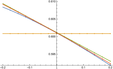
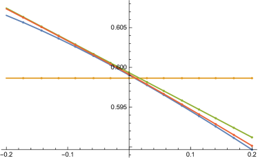
$T=\frac{1}{64}$	$T=\frac{1}{32}$
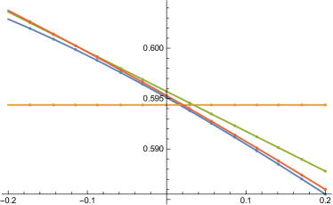
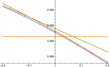
$T=\frac{1}{16}$	$T=\frac{1}{8}$

Figure 1: For the QOU model described in Section 7, we plot exact implied volatility $\sigma$ and approximate implied volatility $\bar{\sigma}_{n}$ up to order $n=2$ as a function of $\log$-moneyness $k-x$ with the initial date and settlement date of the caplet is fixed at $t=0$ and ${\overline{T}}=2$, respectively, and with the reset date of the caplet taking the following values $T=\{\frac{1}{64},\frac{1}{32},\frac{1}{16},\frac{1}{8}\}$. The zeroth, first, and second order approximate implied volatilities correspond to the orange, green and red curves, respectively, and the blue curve corresponds to the exact implied volatility. The following parameters remained fixed: $q=0$, $\kappa=0.9$, $\theta=\frac{0.25}{0.9}$, $\delta=0.2$, $y=\sqrt{0.08}$.

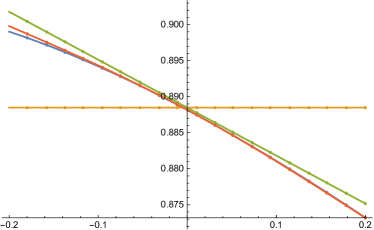
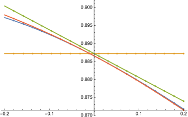
$T=\frac{1}{64}$	$T=\frac{1}{32}$
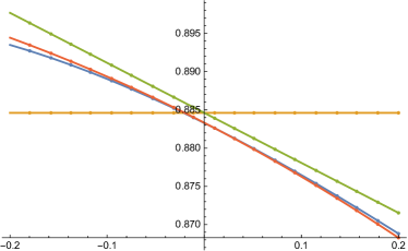
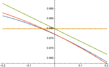
$T=\frac{1}{16}$	$T=\frac{1}{8}$

Figure 2: For the QOU model described in Section 7, we plot the exact implied volatility $\sigma$ and approximate implied volatility $\bar{\sigma}_{n}$ up to order $n=2$ as a function of $\log$-moneyness $k-x$ with the initial date and settlement date of the caplet is fixed at $t=0$ and ${\overline{T}}=2$, respectively, and with the reset date of the caplet taking the following values $T=\{\frac{1}{64},\frac{1}{32},\frac{1}{16},\frac{1}{8}\}$. The zeroth, first, and second order approximate implied volatilities correspond to the orange, green and red curves, respectively, and the blue curve corresponds to the exact implied volatility. The following parameters remained fixed: $\kappa=0.045$, $\delta=\sqrt{0.035}$, $y=\sqrt{0.08}$, $\theta=q=0$.

where we have omitted the 2nd order term $\sigma_{2}$ due to its considerable length.
In Figures 1 and 2, using different parameters for $(\kappa,\theta,\delta,q,y)$, we plot our explicit approximation of implied volatility $\bar{\sigma}_{n}$ up to order $n=2$ as a function of $\log$-moneyness $k-x$ with $t=0$ and ${\overline{T}}=2$ fixed and with reset date ranging over $T=\{\frac{1}{64},\frac{1}{32},\frac{1}{16},\frac{1}{8}\}$. For comparison, we also plot the “exact” implied volatility $\sigma$, which can be computed using ${\overline{T}}$-forward caplet prices using (60) and inverting the Black formula (87) numerically. In both figures, we observe that the second order approximation $\bar{\sigma}_{2}$ accurately matches the level, slope, and convexity of the exact implied volatility $\sigma$ near-the-money for all four reset dates.
In Figures 3 and 4, using the same values for $(\kappa,\theta,\delta,q,y)$ as in Figures 1 and 2, respectively, we plot the absolute value of the relative error of our second order approximation $|\bar{\sigma}_{2}-\sigma|/\sigma$ as a function of $\log$-moneyness $k-x$ and reset date $T$. Consistent with the asymptotic accuracy results (102), we observe that the errors decrease as we approach the origin in both directions of $k-x$ and $T$.

Appendix A Explicit expressions for $\sigma_{0}$, $\sigma_{1}$ and $\sigma_{2}$

In this appendix we give the expressions for the implied volatility approximation using (99) and (100) explicitly up to second order for $d=1$ in terms of the coefficients $c$,$f$,$g$, and $h$ of $\widetilde{\mathscr{A}}$, given in (54), by performing Taylor’s series expansion of the coefficients around $\bar{z}(t)=(x,y)$. To ease the notation, we define

$$\chi_{i,j}(t)\equiv\chi_{i,j}(t,x,y) =\frac{\partial^{i}_{x}\partial^{j}_{y}\chi(t,x,y)}{i!j!}, \chi \in\{c,f,g,h\}.$$ (122)

The zeroth order term $\sigma_{0}$ is given by

$$\sigma_{0} =\sqrt{\frac{2}{T-t}\int_{t}^{T}\mathrm{d}s\,c_{0,0}(s)}.$$ (123)

Next, let us define

$$\mathscr{H}_{n}(\Theta) :=\Big{(}\frac{-1}{\sigma_{0}\sqrt{2(T-t)}}\Big{)}^{n}\mathsf{H}_{n}(\Theta), \Theta :=\frac{x-k-\frac{1}{2}\sigma^{2}_{0}(T-t)}{\sigma_{0}\sqrt{2(T-t)}}.$$ (124)

where $\mathsf{H}_{n}(\Theta)$ is the $n$th-order Hermite polynomial. Then the first order term $\sigma_{1}$ is given by

$$\sigma_{1} =\sigma_{1,0}+\sigma_{0,1},$$ (125)

where $\sigma_{1,0}$ and $\sigma_{0,1}$ are given by

$$\sigma_{1,0} =\frac{1}{(T-t)\sigma_{0}}\int_{t}^{T}\mathrm{d}s\,c_{1,0}(s)\int_{t}^{s}\mathrm{d}q\,c_{0,0}(q)\Big{(}2\mathscr{H}_{1}(\Theta)-1\Big{)},$$ (126)

$$\sigma_{0,1} =\frac{1}{(T-t)\sigma_{0}}\int_{t}^{T}\mathrm{d}s\,c_{0,1}(s)\Big{(}\int_{t}^{s}\mathrm{d}q\,f_{0,0}(q)+\int_{t}^{s}\mathrm{d}q\,h_{0,0}(q)\mathscr{H}_{1}(\Theta)\Big{)}.$$ (127)

Lastly, the second order term $\sigma_{2}$ is given by

$$\sigma_{2} =\sigma_{2,0}+\sigma_{1,1}+\sigma_{0,2},$$ (128)

where the terms $\sigma_{2,0}$, $\sigma_{1,1}$, $\sigma_{0,2}$ are given by

$$\sigma_{2,0} =\frac{1}{(T-t)\sigma_{0}}\bigg{(}\frac{1}{2}\int_{t}^{T}\mathrm{d}s\,c_{2,0}(s)\Big{(}(\int_{t}^{s}\mathrm{d}q\,c_{0,0}(q))^{2}(4\mathscr{H}_{2}(\Theta)-4\mathscr{H}_{1}(\Theta)+1)+2\int_{t}^{s}\mathrm{d}q\,c_{0,0}(q)\Big{)}$$ (129)

$$\quad+\int_{t}^{T}\mathrm{d}s_{1}\,\int_{s_{1}}^{T}\mathrm{d}s_{2}\,c_{1,0}(s_{1})c_{1,0}(s_{2})\Big{(}\int_{t}^{s_{1}}\mathrm{d}q_{1}\,c_{0,0}(q_{1})\int_{t}^{s_{2}}\mathrm{d}q_{2}\,c_{0,0}(q_{2})$$ (130)

$$\quad\times\big{(}4\mathscr{H}_{4}(\Theta)-8\mathscr{H}_{3}(\Theta)+5\mathscr{H}_{2}(\Theta)-\mathscr{H}_{1}(\Theta)\big{)}+\int_{t}^{s_{1}}\mathrm{d}q_{1}\,c_{0,0}(q_{1})\Big{(}6\mathscr{H}_{2}(\Theta)-6\mathscr{H}_{1}(\Theta)+1)\Big{)}\bigg{)}$$ (131)

$$\quad-\frac{\sigma^{2}_{1,0}}{2}\Big{(}(T-t)\sigma_{0}(\mathscr{H}_{2}(\Theta)-\mathscr{H}_{1}(\Theta))+\frac{1}{\sigma_{0}}\Big{)},$$ (132)

$$\sigma_{1,1} =\frac{1}{(T-t)\sigma_{0}}\Bigg{(}\frac{1}{2}\int_{t}^{T}\mathrm{d}s\,c_{1,1}(s)\bigg{(}2\int_{t}^{s}\mathrm{d}q_{1}\,c_{0,0}(q_{1})\int_{t}^{s}\mathrm{d}q_{2}\,h_{0,0}(q_{2})\mathscr{H}_{2}(\Theta)$$ (133)

$$\quad+\int_{t}^{s}\mathrm{d}q_{1}\,c_{0,0}(q_{1})(2\int_{t}^{s}\mathrm{d}q_{2}\,f_{0,0}(q_{2})-\int_{t}^{s}\mathrm{d}q_{2}\,h_{0,0}(q_{2}))\mathscr{H}_{1}(\Theta)$$ (134)

$$\quad-\int_{t}^{s}\mathrm{d}q_{1}\,c_{0,0}(q_{1})\int_{t}^{s}\mathrm{d}q_{2}\,f_{0,0}(q_{2})+\int_{t}^{s}\mathrm{d}q_{1}\,h_{0,0}(q_{1})\bigg{)}$$ (135)

$$\quad+\int_{t}^{T}\mathrm{d}s_{1}\,\int_{s_{1}}^{T}\mathrm{d}s_{2}\,c_{1,0}(s_{1})c_{0,1}(s_{2})\bigg{(}2\int_{t}^{s_{1}}\mathrm{d}q_{1}\,c_{0,0}(q_{1})\int_{t}^{s_{2}}\mathrm{d}q_{2}\,h_{0,0}(q_{2})\mathscr{H}_{4}(\Theta)$$ (136)

$$\quad+\int_{t}^{s_{1}}\mathrm{d}q_{1}\,c_{0,0}(q_{1})\Big{(}2\int_{t}^{s_{2}}\mathrm{d}q_{2}\,f_{0,0}(q_{2})-3\int_{t}^{s_{2}}\mathrm{d}q_{2}\,h_{0,0}(q_{2})\Big{)}\mathscr{H}_{3}(\Theta)$$ (137)

$$\quad+(\int_{t}^{s_{1}}\mathrm{d}q\,c_{0,0}(q)(\int_{t}^{s_{2}}\mathrm{d}q\,h_{0,0}(q)-3\int_{t}^{s_{2}}\mathrm{d}q\,f_{0,0}(q))+\int_{t}^{s_{1}}\mathrm{d}q\,h_{0,0}(q)\Big{)}\mathscr{H}_{2}(\Theta)$$ (138)

$$\quad+\Big{(}\int_{t}^{s_{1}}\mathrm{d}q_{1}\,c_{0,0}(q_{1})\int_{t}^{s_{2}}\mathrm{d}q_{2}\,f_{0,0}(q_{2})-\int_{t}^{s_{1}}\mathrm{d}q_{1}\,h_{0,0}(q_{1})\Big{)}\mathscr{H}_{1}(\Theta)\bigg{)}$$ (139)

$$\quad+\int_{t}^{T}\mathrm{d}s_{1}\,\int_{s_{1}}^{T}\mathrm{d}s_{2}\,c_{0,1}(s_{1})c_{1,0}(s_{2})\bigg{(}2\int_{t}^{s_{1}}\mathrm{d}q_{1}\,h_{0,0}(q_{1})\int_{t}^{s_{2}}\mathrm{d}q_{2}\,c_{0,0}(q_{2})\mathscr{H}_{4}(\Theta)$$ (140)

$$\quad+\Big{(}2\int_{t}^{s_{1}}\mathrm{d}q_{1}\,f_{0,0}(q_{1})-3\int_{t}^{s_{1}}\mathrm{d}q_{1}\,h_{0,0}(q_{1})\Big{)}\int_{t}^{s_{2}}\mathrm{d}q_{2}\,c_{0,0}(q_{2})\mathscr{H}_{3}(\Theta)$$ (141)

$$\quad+\Big{(}\big{(}\int_{t}^{s_{1}}\mathrm{d}q_{1}\,h_{0,0}(q_{1})-3\int_{t}^{s_{1}}\mathrm{d}q_{1}\,f_{0,0}(q_{1})\big{)}\int_{t}^{s_{2}}\mathrm{d}q_{2}\,c_{0,0}(q_{2})+3\int_{t}^{s_{1}}\mathrm{d}q_{1}\,h_{0,0}(q_{1})\Big{)}\mathscr{H}_{2}(\Theta)$$ (142)

$$\quad+\Big{(}\int_{t}^{s_{1}}\mathrm{d}q_{1}\,f_{0,0}(q_{1})(2+\int_{t}^{s_{2}}\mathrm{d}q_{2}\,c_{0,0}(q_{2}))-2\int_{t}^{s_{1}}\mathrm{d}q_{1}\,h_{0,0}(q_{1})\Big{)}\mathscr{H}_{1}(\Theta)-\int_{t}^{s_{1}}\mathrm{d}q_{1}\,f_{0,0}(q_{1})\bigg{)}$$ (143)

$$\quad+\int_{t}^{T}\mathrm{d}s_{1}\,\int_{s_{1}}^{T}\mathrm{d}s_{2}\,f_{1,0}(s_{1})c_{0,1}(s_{2})\int_{t}^{s_{1}}\mathrm{d}q_{1}\,c_{0,0}(q_{1})\Big{(}2\mathscr{H}_{1}(\Theta)-1\Big{)}$$ (144)

$$\quad+2\int_{t}^{T}\mathrm{d}s_{1}\,\int_{s_{1}}^{T}\mathrm{d}s_{2}\,h_{1,0}(s_{1})c_{0,1}(s_{2})\int_{t}^{s_{1}}\mathrm{d}q_{1}\,c_{0,0}(q_{1})\Big{(}2\mathscr{H}_{2}(\Theta)-\mathscr{H}_{1}(\Theta)\Big{)}\Bigg{)}$$ (145)

$$\quad-\sigma_{1,0}\sigma_{0,1}\Big{(}(T-t)\sigma_{0}(\mathscr{H}_{2}(\Theta)-\mathscr{H}_{1}(\Theta))+\frac{1}{\sigma_{0}}\Big{)},$$ (146)

$$\sigma_{0,2} =\frac{1}{(T-t)\sigma_{0}}\Bigg{(}\frac{1}{2}\int_{t}^{T}\mathrm{d}s\,c_{0,2}(s)\bigg{(}\Big{(}\int_{t}^{s}\mathrm{d}q\,h_{0,0}(q)\big{)}^{2}\mathscr{H}_{2}(\Theta)+2\int_{t}^{s}\mathrm{d}q_{1}\,h_{0,0}(q_{1})\int_{t}^{s}\mathrm{d}q_{2}\,f_{0,0}(q_{2})\mathscr{H}_{1}(\Theta)$$ (147)

$$\quad+(\int_{t}^{s}\mathrm{d}q\,f_{0,0}(q))^{2}+2\int_{t}^{s}\mathrm{d}q\,g_{0,0}(q)\bigg{)}$$ (148)

$$\quad+\int_{t}^{T}\mathrm{d}s_{1}\,\int_{s_{1}}^{T}\mathrm{d}s_{2}\,c_{0,1}(s_{1})c_{0,1}(s_{2})\bigg{(}\int_{t}^{s_{1}}\mathrm{d}q_{1}\,h_{0,0}(q_{1})\int_{t}^{s_{2}}\mathrm{d}q_{2}\,h_{0,0}(q_{2})\mathscr{H}_{4}(\Theta)$$ (149)

$$\quad+\Big{(}\int_{t}^{s_{1}}\mathrm{d}q_{1}\,f_{0,0}(q_{1})\int_{t}^{s_{2}}\mathrm{d}q_{2}\,h_{0,0}(q_{2})+\int_{t}^{s_{1}}\mathrm{d}q_{1}\,h_{0,0}(q_{1})\int_{t}^{s_{2}}\mathrm{d}q_{2}\,f_{0,0}(q_{2})$$ (150)

$$\quad-\int_{t}^{s_{1}}\mathrm{d}q_{1}\,h_{0,0}(q_{1})\int_{t}^{s_{2}}\mathrm{d}q_{2}\,h_{0,0}(q_{2})\Big{)}\mathscr{H}_{3}(\Theta)$$ (151)

$$\quad+\Big{(}2\int_{t}^{s_{1}}\mathrm{d}q\,g_{0,0}(q)+\int_{t}^{s_{1}}\mathrm{d}q_{1}\,f_{0,0}(q_{1})\int_{t}^{s_{2}}\mathrm{d}q_{2}\,f_{0,0}(q_{2})-\int_{t}^{s_{1}}\mathrm{d}q_{1}\,f_{0,0}(q_{1})\int_{t}^{s_{2}}\mathrm{d}q_{2}\,h_{0,0}(q_{2})$$ (152)

$$\quad-\int_{t}^{s_{2}}\mathrm{d}q_{1}\,f_{0,0}(q_{1})\int_{t}^{s_{1}}\mathrm{d}q_{2}\,h_{0,0}(q_{2})\Big{)}\mathscr{H}_{2}(\Theta)$$ (153)

$$\quad-\Big{(}2\int_{t}^{s_{1}}\mathrm{d}q\,g_{0,0}(q)+\int_{t}^{s_{1}}\mathrm{d}q_{1}\,f_{0,0}(q_{1})\int_{t}^{s_{2}}\mathrm{d}q_{2}\,f_{0,0}(q_{2})\Big{)}\mathscr{H}_{1}(\Theta)\bigg{)}$$ (154)

$$\quad+\int_{t}^{T}\mathrm{d}s_{1}\,\int_{s_{1}}^{T}\mathrm{d}s_{2}\,f_{0,1}(s_{1})c_{0,1}(s_{2})\Big{(}\int_{t}^{s_{1}}\mathrm{d}q\,h_{0,0}(q)\mathscr{H}_{1}(\Theta)+\int_{t}^{s_{1}}\mathrm{d}q\,f_{0,0}(q)\Big{)}$$ (155)

$$\quad+\int_{t}^{T}\mathrm{d}s_{1}\,\int_{s_{1}}^{T}\mathrm{d}s_{2}\,h_{0,1}(s_{1})c_{0,1}(s_{2})\Big{(}\int_{t}^{s_{1}}\mathrm{d}q\,h_{0,0}(q)\mathscr{H}_{2}(\Theta)+\int_{t}^{s_{1}}\mathrm{d}q\,f_{0,0}(q)\mathscr{H}_{1}(\Theta)\Big{)}\Bigg{)}$$ (156)

$$\quad-\frac{\sigma^{2}_{0,1}}{2}\Big{(}(T-t)\sigma_{0}(\mathscr{H}_{2}(\Theta)-\mathscr{H}_{1}(\Theta))+\frac{1}{\sigma_{0}}\Big{)}.$$ (157)

Note that, although $\mathscr{H}_{3}(\Theta)$ and $\mathscr{H}_{4}(\Theta)$ appear in the expressions for $\sigma_{2,0},\sigma_{1,1}$ and $\sigma_{0,2}$, the 3rd and 4th order terms in $k-x$ cancel the 3rd and 4th order terms resulting from $\{\sigma_{1,0}^{2}\mathscr{H}_{2}(\Theta),\sigma_{1,0}^{2}\mathscr{H}_{1}(\Theta)\}$, $\{\sigma_{0,1}\sigma_{1,0}\mathscr{H}_{2}(\Theta),\sigma_{0,1}\sigma_{1,0}\mathscr{H}_{1}(\Theta)\}$, and $\{\sigma_{0,1}^{2}\mathscr{H}_{2}(\Theta),\sigma_{0,1}^{2}\mathscr{H}_{1}(\Theta)\}$, respectively, resulting in a second order implied volatility expansion that is quadratic in $k-x$.

Figure 3: For the QOU model described in Section 7, we plot the absolute value of the relative error of our second order implied volatility approximation $|\bar{\sigma}_{2}-\sigma|/\sigma$ as a function of $\log$-moneyness $k-x$ and caplet reset date $T$. The horizontal axis represents $\log$-moneyness $k-x$ and the vertical axis represents caplet reset date $T$. Ranging from darkest to lightest, the regions above represent relative errors in increments of $0.002$ from $<0.002$ to $>0.018$. The initial date and settlement date of the caplet is fixed at $t=0$ and ${\overline{T}}=2$, respectively. The following parameters remained fixed: $q=0$, $\kappa=0.9$, $\theta=\frac{0.25}{0.9}$, $\delta=0.2$, $y=\sqrt{0.08}$.

Figure 4: For the QOU model described in Section 7, we plot the absolute value of the relative error of our second order implied volatility approximation $|\bar{\sigma}_{2}-\sigma|/\sigma$ as a function of $\log$-moneyness $k-x$ and caplet reset date $T$. The horizontal axis represents $\log$-moneyness $k-x$ and the vertical axis represents caplet reset date $T$. Ranging from darkest to lightest, the regions above represent relative errors in increments of $0.005$ from $<0.005$ to $0.03$. The initial date and settlement date of the caplet is fixed at $t=0$ and ${\overline{T}}=2$, respectively. The following parameters remained fixed: $\kappa=0.045$, $\delta=\sqrt{0.035}$, $y=\sqrt{0.08}$, $\theta=q=0$.

References

- Ahn et al. [2002] D.-H. Ahn, R. F. Dittmar, and A. R. Gallant. Quadratic term structure models: Theory and evidence. The Review of financial studies, 15(1):243–288, 2002.
- Angelini and Herzel [2006] F. Angelini and S. Herzel. Notes and comments: An approximation of caplet implied volatilities in gaussian models. Decisions in Economics and Finance, 28(2):113–127, 2006.
- Barletta et al. [2019] A. Barletta, E. Nicolato, and S. Pagliarani. The short-time behavior of vix-implied volatilities in a multifactor stochastic volatility framework. Mathematical Finance, 29(3):928–966, 2019.
- Chen et al. [2004] L. Chen, D. Filipović, and H. V. Poor. Quadratic term structure models for risk-free and defaultable rates. Mathematical Finance: An International Journal of Mathematics, Statistics and Financial Economics, 14(4):515–536, 2004.
- Cox et al. [2005] J. C. Cox, J. E. Ingersoll Jr, and S. A. Ross. A theory of the term structure of interest rates. In Theory of valuation, pages 129–164. World Scientific, 2005.
- Hull and White [1990] J. Hull and A. White. Pricing interest-rate-derivative securities. The review of financial studies, 3(4):573–592, 1990.
- Leung et al. [2017] T. Leung, M. Lorig, and A. Pascucci. Leveraged etf implied volatilities from etf dynamics. Mathematical Finance, 27(4):1035–1068, 2017.
- Lorig and Suaysom [2022] M. Lorig and N. Suaysom. Options on bonds: implied volatilities from affine short-rate dynamics. Annals of Finance, pages 1–34, 2022.
- Lorig et al. [2015] M. Lorig, S. Pagliarani, and A. Pascucci. Analytical expansions for parabolic equations. SIAM Journal on Applied Mathematics, 75:468–491, 2015.
- Lorig et al. [2017] M. Lorig, S. Pagliarani, and A. Pascucci. Explicit implied volatilities for multifactor local-stochastic volatility models. Mathematical Finance, 27(3):926–960, 2017. ISSN 1467-9965. doi: 10.1111/mafi.12105. URL http://dx.doi.org/10.1111/mafi.12105.
- Pagliarani and Pascucci [2012] S. Pagliarani and A. Pascucci. Analytical approximation of the transition density in a local volatility model. Cent. Eur. J. Math., 10(1):250–270, 2012. ISSN 1895-1074. doi: 10.2478/s11533-011-0115-y. URL http://dx.doi.org/10.2478/s11533-011-0115-y.
- Shreve [2004] S. E. Shreve. Stochastic calculus for finance II: Continuous-time models, volume 11. Springer Science & Business Media, 2004.
- Vasicek [1977] O. Vasicek. An equilibrium characterization of the term structure. Journal of financial economics, 5(2):177–188, 1977.