TESS light curves of cataclysmic variables – II – Superhumps in old novae and novalike variables

Abstract

Superhumps are among the abundant variable phenomena observed in the light curves of cataclysmic variables (CVs). They come in two flavours as positive and negative superhumps, distinguished by periods slightly longer or shorter, respectively, than the orbital periods of these interacting binary systems. Positive superhumps are ubiquitous in superoutbursting short period dwarf novae of the SU UMa type but are less common in longer period systems with accretion disks in a permanent bright state such as novalike variables and most old novae. Negative superhumps do not seem not to have a preference for a particular type of CV. Here, I take advantage of the long high cadence light curves provided by TESS for huge number of stars, selecting all old novae and novalike variables with past reported superhumps for which TESS light curves are available and have not yet been analysed in previous publications in order to study their superhump behaviour. In combination with information taken from the literature the results enable to compile the most complete census of superhumps in these stars so far. As a corollary, for the eclipsing systems in the present sample of objects eclipse epochs derived from the TESS light curves and in some cases from archival light curves are listed and used to update orbital ephemeris and to discuss period changes.

1 Introduction

Variability in cataclysmic variables (CVs) occurs in a multitude of different forms and on a wide range of time scales. Most of it is associated to mass transfer or aspect variations in these close binary systems composed of a white dwarf primary star and a Roche-lobe filling late type secondary component transferring matter to the primary which – in the absence of a strong magnetic field of the white dwarf – forms an accretion disk around the compact star before it is accreted onto its surface.

A good characterization of many of the variable phenomena requires extensive observations of the respective stars with a suitable time resolution over as long a time base as possible. In this respect the long continuous high cadence light curves provided by the Kepler mission have been extremely beneficial (e.g., Osaki & Kato, 2013; Ramsay et al., 2016; Bruch, 2022a, to cite only a few examples). However, Kepler observed but a few CVs. This changed considerably with the launch of the Transit Exoplanet Survey Satellite (TESS, Ricker et al., 2014) which – although equipped with much smaller telescopes and pointing at a given sector of the sky for less time – provided light curves of many more CVs with a time base and a temporal resolution well suited to address many issues concerning the variability in these stars.

A particular type of consistent modulations in numerous CVs are the so-called superhumps (SHs); i.e., variations with a period a few percent different from the orbital period of the binary. SHs come in two flavours: positive superhumps (pSHs) with periods slightly longer than the orbital period, and negative superhumps (nSHs) the periods of which are a bit shorter than the orbit.

pSHs were first observed in dwarf nova type CVs of the SU UMa subclass during superoutburst (Vogt, 1974) and have since become the hallmark of this particular outburst stage of SU UMa stars (Kato et al., 2009, and other publications of this series). pSHs are thought to arise when the accretion disk expands such that the revolution period of matter at its outer rim reaches the 3:1 resonance radius with the binary orbit. This condition is most easily attained during large scale (super-) outbursts in short period dwarf novae, i.e., SU UMa stars. The tidal interaction of the disk with the secondary star then induces an elliptical deformation in the former (Whitehurst, 1988; Whitehurst & King, 1991). Whenever the secondary star passes close to the elongated part of the disk tidal, stresses cause an increase of the disk luminosity. This occurs on a period slightly longer than the orbital period because of a prograde precession of the deformed disk.

pSHs are not restricted to SU UMa stars in superoutburst but are also observed in increasing number in non-outbursting CVs such as novalike variables (NLs) and old novae (which have an accretion disk in a similar state as the NLs). Most of these have periods longer than the SU UMa stars. Since the secondary star mass in CVs increases systematically with the orbital period their mass ratio $q=M_{\rm prim}/M_{\rm sec}$ is on average also higher and may reach (or even surpass, see Sect. 4) the theoretical limit for the condition required to generate SHs. This limit is contested but appears to lie somewhere in the range $q=0.22\ldots 0.39$ (Whitehurst & King, 1991; Pearson, 2006; Smak, 2020).

While the basic physics of pSHs are thus thought to be reasonably well understood, this is not the case for negative superhumps. Phenomenologically, they are explained to arise in a warped accretion disk or a disk inclined with respect to the orbital plane. In such a configuration, depending on the variable aspect between the disk and the stream of infalling matter from the secondary star, the latter penetrates more or less deeply into the gravitational well of the white dwarf before its hits the accretion disk and thus liberates a variable amount of energy, leading to a modulation of the disk luminosity. The inclined disk precesses retrogradely such that the same aspect between the disk and the infalling stream of matter repeats on a period slightly less than the orbital period. While this scenario is widely accepted to explain nSHs there is no consensus about the mechanism which causes a warp or an inclination of the accretion disk in the first place (Montgomery, 2009; Thomas & Wood, 2015). Thus, there are no theoretical constraints for the appearance of nSHs. Observationally, they are found in short period dwarf novae (Wood et al., 2011; Osaki & Kato, 2014) as well as in long period NLs (Kimura et al., 2020).

The periods of both, pSHs and nSHs, are not strictly constant but exhibit small variations depending on details of the distribution of mass within the the accretion disk.

Recently, Bruch (2022b) (hereafter referred to as Paper I) investigated the TESS light curves of a sample of NLs and old novae and identified SHs in several systems which were hitherto not known to be superhumpers. In extension of that study I investigate here the TESS light curves of all NLs and old novae with SHs, either positive or negative, reported in the literature which have been observed by TESS, and the TESS data of which have not already been the subject of other publications. The data used and methods applied are briefly outlined in Sect. 2. Thereafter, the individual systems are discussed in Sect. 3. For some eclipsing CVs additional eclipse epochs, an update of the orbital period, and an assessment of period variations are also included as a corollary. In Sect. 4, I present a census of all superhumping NLs and old novae. A summary of the results concludes this study in Sect. 5.

2 Data and data handling

The details of the data used in this study and their handling are largely the same as in Paper I and were described there. Therefore, I will only give a summary here. TESS SAP data with a time resolution of 2 min were downloaded from the Barbara A. Misulski Archive for Space Telescopes (MAST). For one object (KIC 8751494) data from the Kepler mission, retrieved from the same source, are also used. Whenever observations from different TESS sectors were obtained in immediate succession they were combined into a single light curve. Different light curves of the same object are referred to as LC#1, LC#2, etc. The start and end epochs of the light curves are listed in Table 1.

Table 1: Journal of observations.

Name	LC	Start time	End time
	number	BJD 2450000+
PX And	1	8764.69	8788.92
UU Aqr	1	9447.70	9473.16
KR Aur	1	9474.17	9550.63
BZ Cam	1	8816.88	8868.83
	2	9010.26	9035.13
	3	9390.65	9418.85
V592 Cas	1	8764.69	8789.68
	2	8955.79	8982.27
RR Cha	1	9333.86	9389.72
V751 Cyg	1	8711.37	5737.41
V1974 Cyg	1	8738.65	8763.32
	2	9418.99	9446.58
BB Dor	1	8325.29	8682.36
	2	9036.28	9389.72
BH Lyn	1	8842.51	8868.83
	2	9579.82	9606.94
BK Lyn	1	8870.44	8897.79
AH Men	1	8325.30	8353.17
	2	8410.90	8436.83
	3	8596.78	8682.36
	4	9036.28	9060.64
	5	9333.86	9389.72
RR Pic	1	8354.11	8595.68
	2	8624.97	8682.36
	3	9036.28	9060.64
	4	9088.24	9332.58
	5	9361.29	9389.72
AO Psc	1	9447.70	9473.16
AY Psc	1	9447.69	9498.81
V348 Pup	1	9201.74	9254.07
RW Tri	1	8790.66	8814.27
UX UMa	1	8711.36	8763.32
	2	8899.32	8954.88
DW UMa	1	8870.46	8897.78
	2	9607.94	9635.97
HS 1813+6122	1	8683.35	8841.14
	2	8870.17	9037.40
	3	9419.99	9456.58
	4	9579.81	9664.31
RX J2133.7+5107	1	8711.36	8763.32
KIC 8751494	1	8711.37	8737.41
	2	9390.66	9446.58
KIC 9406652	1	8683.36	8710.21
	2	8711.37	8737.41
	3	8085.66	9446.58
NSV 1907	1	9174.23	9200,23

Frequency analysis of the data were performed with Fourier techniques applying the Lomb-Scargle algorithm (Lomb, 1976; Scargle, 1982) or following Deeming (1975). Unless variations on longer time scales were targeted these were removed by subtraction of a Savitzky & Golay (1964) filtered version of the light curve, using a cut-off time scale of 2 d and a 4^th order smoothing polynomial for the filter. The frequency errors of power spectrum signals were estimated using the prescription of Schwarzenberg-Czerny (1991) which due to flickering and window patterns of real variations may overestimate the true errors.

Comparing TESS light curves with terrestial data it should be kept in mind that the TESS passband encompasses a wide range between 6 000 and 10 000 Å, centred on the Cousins $I$-band.

For the deeply eclipsing CVs in the present sample eclipse epochs were measured to enable an update of the orbital ephemeris and for future reference. Instead of measuring individual eclipse timings the light curves were folded on the orbital period, choosing the epoch such that the centre of the primary eclipse coincides with phase 0. This was done individually for the data of each TESS sector, yielding more than one eclipse epoch for the light curves combined from several sectors. The corresponding results are listed in Table 2. For four CVs (UU Aqr, V348 Pup, RW Tri and UX UMa) additional eclipse epochs were measured in light curves downloaded from the American Association of Variable Star Observers (AAVSO) archives (Kafka, 2021) and the data bank of the Observatório do Pico dos Dias (LNA Data Bank) as the minima of polynomials of suitable degree fitted to the eclipse profiles. They are listed in Appendix A. The transformation from JD to BJD was performed using the on-line tool of Eastman et al. (2010).

3 Results

Table 2: Representative eclipse epochs.

Star	Light curve	Epoch (BJD)	Cycle number1
PX And	LC#1	2458779.1330	65187
UU Aqr	LC#1	2459462.1633	47111
RR Cha	LC#1	2459363.0160	0
AH Men	LC#1	2458340.0867	0
	LC#2	2458425.0527	668
	LC#3 (part 1)	2458611.0146	2130
	LC#3 (part 2)	2458646.1193	2406
	LC#3 (part 3)	2458671.0497	2602
	LC#4	2459051.1099	5590
	LC#5 (part 1)	2459348.1110	7925
	LC#5 (part 2)	2459373.0414	8121
BH Lyn	LC#1	2458857.1359	74911
	LC#2	2459591.1530	79620
AY Psc	LC#1 (part 1)	2459462.1062	54476
	LC#1 (part 2)	2459488.1850	54596
V348 Pup	LC#1 (part 1)	2459211.0279	104276
	LC#1 (part 2)	2459238.0154	104541
RW Tri	LC#1	245880.0263	22112
UX UMa	LC#1 (part 1)	2458726.0252	37658
	LC#1 (part 2)	2458746.0858	37760
	LC#2 (part 1)	2458914.0431	38614
	LC#2 (part 2)	2458944.1338	38767
DW UMa	LC#1	2458885.0575	56178
	LC#2	2459622.0503	61573
HS 1813-6122	LC#1 (part 1)	2458693.0878	0
	LC#1 (part 2)	2458723.0351	203
	LC#1 (part 3)	2458753.1285	407
	LC#1 (part 4)	2458773.0430	542
	LC#1 (part 5)	2458803.1372	746
	LC#1 (part 6)	2458833.0826	949
	LC#2 (part 1)	2458880.1437	1268
	LC#2 (part 2)	2458910.0900	1471
	LC#2 (part 3)	2458940.0367	1674
	LC#2 (part 4)	2458970.1298	1878
	LC#2 (part 5)	2459000.0758	2081
	LC#2 (part 6)	2459020.1399	2217
	LC#3	2459429.0664	4989
	LC#4 (part 1)	2459589.1243	6074
	LC#4 (part 3)	2459649.0186	6480
NSV 1907	LC#1	2459189.1635	7710

¹ cycle count convention according to: this work (UU Aqr, RR Cha, AH Men, RW Tri, UX UMa, HS 1813-6122); Hellier & Robinson (1994) (PX And); Andronov et al. (1989) (BH Lyn); Diaz & Steiner (1990) (AY Psc); Dai et al. (2010) (V348 Pup); Boyd et al. (2017) (DW UMa); Hümmerich et al. (2017) (NSV 1907)

3.1 PX And: no superhumps in the TESS light curve

PX And is an eclipsing novalike variable. Stanishev et al. (2002) derived the most accurate value for the orbital period: 0.146352739(11) d. The same authors also found a periodic variation at 0.1415 d which they attribute to a nSH, and another one at 0.207 d the origin of which remained unexplained. The only significant signals in the power spectrum of the single TESS light curve correspond to the orbital period and its overones. Fig. 1a shows the frequency range around the orbital signal (which is truncated in order to better visualize any faint signals in its vicinity). No trace of a SH, either positive or negative, or of the 0.207 d period appears. Their frequencies are marked by red arrows in the figure. A representative eclipse epoch derived from the TESS data is listed in Table 2.

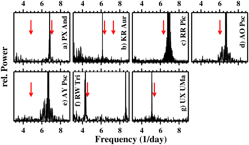
Figure 1: Power spectra in the range around the orbital frequency of six CVs with superhumps reported in the past but with no indications for superhumps in the TESS light curves. The orbital signals are heavily truncated in order to better visualize any faint signals in their vicinity. The frequencies of previously identified periodic signals are marked with red arrows. Note that the broad base around the orbital frequency (in particular in the RR Pic, AO Psc and AY Psc power spectra) are not independent signals but the unavoidable sidelobes of the main peak.

3.2 UU Aqr: The superhump vanished

UU Aqr is an eclipsing novalike variable. Although known as a variable star for almost a century (Beljawsky, 1926) it was identified as a CV only in 1986 by Volkov et al. (1986). Superhumps were observed by Patterson et al. (2005) but were absent in extensive photometry of Bruch (2019a). Lima et al. (2021) make no mention of SHs but claim to see a photometric period of 54.4 min, and of 25.7 min in circular polarization.

TESS observed UU Aqr in a single sector. The power spectrum of the light curve, after masking eclipses and removing variations on time scale above 2 d, is shown in the upper frame of Fig. 2. In the low ($<$20 d^-1) frequency range the orbital signal and the first two overtones stand out moderately strong above a multitude of peaks with decreasing power towards higher frequencies which can be attributed to non-coherent fluctuations in the brightness of UU Aqr on time scales of hours. An increase of power between 10 and 11 d^-1 may be significant. No outstanding signal is present near 5.711 d^-1 (marked by a red arrow in the figure), i.e., the frequency of the SH which is so prominent in the observations of Patterson et al. (2005) (see their figure 3). Thus, the superhump was not active during the epoch of the TESS observations.

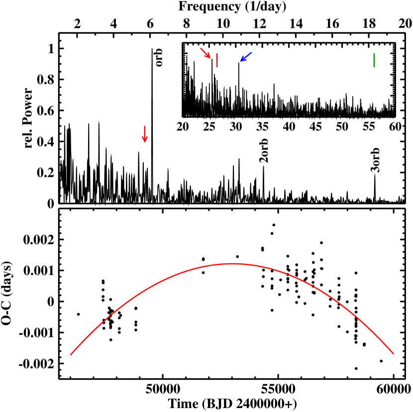
Figure 2: Top: Low frequency part of the power spectrum of the UU Aqr light curve. The insert shows the adjacent higher frequency part at on expanded power scale. The marks drawn into the figure are explained in the text. Bottom: $O-C$ diagram of eclipse timings of UU Aqr with respect to linear ephemeris according to Eq. 1. The red graph represents the best fit second order polynomial.

At higher frequencies (insert in Fig. 2) the fourth overtone of $F_{\rm orb}$ is the only signal which can be attributed to orbital variations (blue arrow). A stronger signal at 25.55 d^-1 ($P=56.36$ min; red arrow) is distinct from the third orbital overtone, but is possibly related to the 54.4 min photometric periodicity mentioned by Lima et al. (2021). Although the corresponding frequency (red bar) is somewhat higher, the power spectrum in figure 7 of Lima et al. (2021) contains numerous alias peaks reaching out until well beyond 56.36 min. I note, however, that the light curves of Bruch (2019a) do not contain an indication for variations in this period range. On the other hand, the power spectrum of those data has a marginally significant peak compatible with the 25.7 min polarimetric period which Lima et al. (2021) take as an indication for an intermediate polar nature of UU Aqr. But no such signal can be discerned in the TESS data (green bar in Fig. 2).

The orbital period of UU Aqr was last refined by Baptista et al. (1995) almost 30 yr ago. It is based on eclipse epoch measurements over a time base of about 7 yr. I am not aware of any published eclipse timings since then which would enable to enlarge the time base for period determination. A representative eclipse epoch derived from the TESS light curve is listed in Table 2. The AAVSO archives and the LNA Data Bank contain many more time resolved light curves of UU Aqr observed between 2000 and 2019 which can be used to measure additional eclipse timings. After rejecting a couple of eclipses because their timings led to excessive $O-C$ values, I am left with 99 additional eclipse epochs which are listed in Table A1. These new data extend the time base for period determination by more than a factor of 5.

Combining the new eclipse timings with those listed by Baptista et al. (1994), (assigning weight 10 to the TESS eclipse epoch because it is based on many individual eclipses, and 1 to all others), neglecting the slight difference between BJD and HJD used in the earlier publications, and choosing an epoch close to the centre of all available eclipse epochs as zero point for cycle counts, the revised linear orbital ephemeris for UU Aqr are:

$$T_{\rm min}=BJD\,2451755.72717(8)+0.163580440(2)\times E$$ (1)

The resulting $O-C$ curve for the eclipse epochs are plotted in the lower frame of Fig. 2. There is a clear trend over time which can very well be described by a parabola, indicating that the orbital period of UU Aqr changes gradually over time. Thus, the eclipse epochs are better described by quadratic ephemeris:

$$T_{\rm min} = BJD\,2451755.72834(4)$$

$$+0.163580465(1)\times E$$

$$-1.84(4)\,10^{-12}\times E^{2}$$

The period decreases currently at a rate of ${\rm d}P/{\rm d}t=-2.240(4)\times 10^{-11}$ and the relative period decrease is $\dot{P}/P=5.010(9)\times 10^{-8}$ yr^-1.

3.3 KR Aur: The superhumps subsided

KR Aur is a well known novalike variable of the VY Scl subtype. The long term behaviour has been extensively monitored in the literature (see, e.g., Honeycutt & Kafka, 2004). For the early history of the system, see Kato et al. (2002). The orbital period was measured spectroscopically by Hutchings et al. (1983) and Shafter (1983) and more recently photometrically by Rodríguez-Gil et al. (2020) who provide the most accurate value of 0.162771641(49) d. Apart from the frequent low states which characterize KR Aur as a VY Scl star the system exhibits variability also on short time scales, i.e., the usual flickering seen in all CVs, but stronger than in most NLs (Bruch, 2021). Significant signals with unstable periods on the time scale of several hundred seconds have been seen by Singh et al. (1993) and Kato et al. (2002). Biryukov & Borisov (1990) claim the presence of 25 min variations, but these are quite unstable and can at most be classified as quasi-periodic oscillations (QPOs). In contrast, Kozhevnikov (2007) reports the presence in 2004, January and February, of a nSH at a period of 0.15713(2) d. Similar signals were, however, not detected in observations of Kato et al. (2002). In contrast, more recently, in 2021 January, Boeva et al. (2021) observed a nSH at a period of 0.1367(2) d, significantly shorter than that seen by Kozhevnikov (2007). All these observations were performed in high states.

Some months later, between September and November of the same year, again in a high state, TESS observed KR Aur in three sectors in subsequent time intervals. Apart from multiple signals at frequencies $<$4 d^-1 due to random variations on longer time scales, only a strong signal at the orbital frequency is outstanding. No indications for superhumps can be detected (Fig. 1b). Thus, the variations seen by Boeva et al. (2021) had subsided. The appearance of superhumps in KR Aur is consequently not permanent but an intermittent phenomenon. Moreover, the high frequency part of the power spectrum does not contain power in excess of the usual red flickering noise on the times scales indicated by Singh et al. (1993), Kato et al. (2002) or Biryukov & Borisov (1990).

3.4 BZ Cam: Lots of unstable signals

The long term photometric behaviour of BZ Cam, classified as a novalike variable, is somewhat unusual for its class. For many years it remained at a seemingly stable magnitude of $\sim$13 after a low state at $\sim$14 mag in 1928 (Garnavich & Szkody, 1988). Another low state occurred in 1999 (Greiner et al., 2001; Kato & Uemura, 2001). This would make BZ Cam a typical VY Scl star. But the AAVSO long term light curve, starting in late 2000, contains several excursions to a brighter state around 12 mag (apart from a short glitch to the low state level).

Combining spectroscopic and photometric data Patterson et al. (1996) derived an orbital period of 0.153693(7) d. They also saw very complicated structures in the power spectra of their light curves with a concentration of multiple signals in the frequency range below $\sim$20 d^-1. They tried to isolate specific signals and to discuss them in terms of positive and negative SHs, but admitted that their interpretation is not unique. Kato & Uemura (2001), in contrast, claim the presence of a pSH at 0.15634(1) during the 1999 low state of BZ Cam.

The TESS observations of BZ Cam can be combined into three light curves. Their power spectra (upper frames of Fig. 3) are similar to those shown by Patterson et al. (1996) with a concentration of peaks in the range between 8 and 14 d^-1 (periods between 1.7 and 3 h). The orbital frequency is marked by red vertical bars in the figure. Orbital variations clearly manifest themselves in LC#1 and LC#3, but are absent in LC#2. No trace of the SH seen by Kato & Uemura (2001) is present in the power spectra.

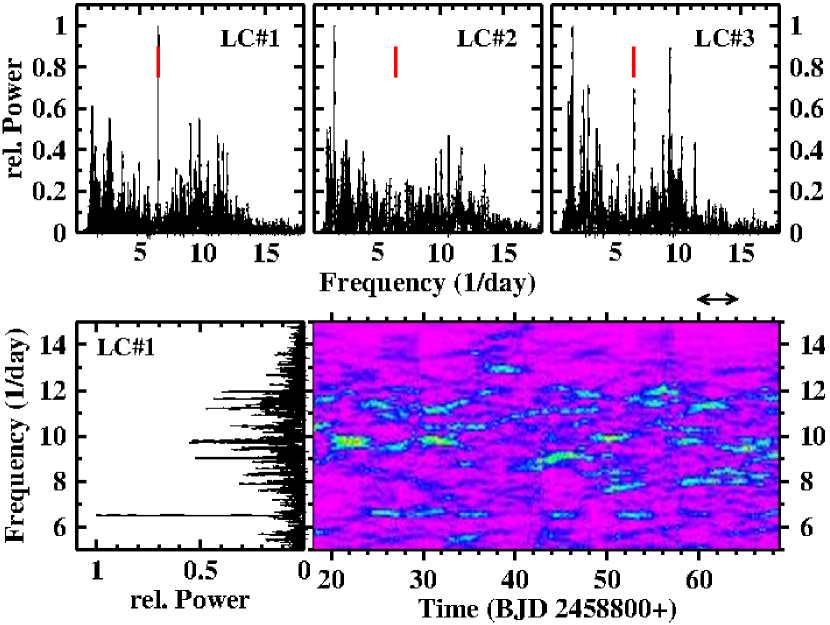
Figure 3: Top: Power spectra of the light curves of BZ Cam. the red vertical lines indicate the orbital frequency. Bottom: Part of the power spectrum of LC#1 in a conventional representation (left) together with a three dimensional plot of the power (colour coded) as a function of frequency and time (right). The double arrow above the plot indicates the width of the time intervals used to calculate the power spectrum and thus its time resolution.

In order to further investigate the occurrence of multiple apparently quite unstable periods of a few hours, time resolved power spectra were calculated using a sliding window with a widths of 4 d. The results for LC#1 are shown in the lower right frame of Fig. 3 (those for the other light curves are qualitatively similar). For comparison, the conventional power spectrum of the entire light curve is reproduced in the left frame. The time resolved spectrum is dominated by a profusion of signals which appear at random, vanish after a couple of days and can change their frequency during their life time. This is the typical behaviour of QPOs which are not uncommon in CVs but normally have shorter periods in the range of minutes to some tens of minutes. Their behaviour in BZ Cam is, however, somewhat reminiscent of CP Pup (see Paper I). These QPOs having been seen by Patterson et al. (1996) in 1994-95 and by TESS between 2019 and 2021 suggest that they are a permanent property of BZ Cam.

Another interesting feature in the time resolved power spectrum is the coming and going of the orbital signal which semi-periodically appears and vanishes on the time scale of several days.

3.5 V592 Cas: No nSH and drastically changed pSH waveform

V592 Cas was discovered by Greenstein et al. (1970) as LSI 55^o-8. The orbital period was measured spectroscopically to be 0.115063(1) d by Taylor et al. (1998). The latter authors also found strong pSHs at a period of 0.12228(1) d. Additionally, in 1997-1998 they saw a weak signal at 0.11193(5) d which they interpreted as a nSH. This was not detected in the 1993 observing season.

The overall properties of the two available TESS light curves taken about 6 months apart are similar. The upper frame of Fig. 4 shows LC#2. It is characterized by regular but non periodic variations on the time scale of a day. This is reflected in the power spectra in the lower left frame of the figure which contains numerous peaks at frequencies below 4 d^-1. A faint peak corresponding to a period of 0.1151(1) d in both power spectra can be identified with the orbital period of V592 Cas. I consider another signal at a slightly lower frequency, corresponding to a period of 0.1225(1) d, very similar to that reported by Taylor et al. (1998), as being caused by a positive superhump. However, its first overtone is vastly stronger. This is explained by the SH waveform shown in the lower right frame of Fig. 4 which consists of two maxima separated by minima of quite different depth. Except for a reversal of the slightly different heights of the two maxima, the waveform is the same in both lightcurves. It is drastically different from the simple saw-tooth shape observed by Taylor et al. (1998).

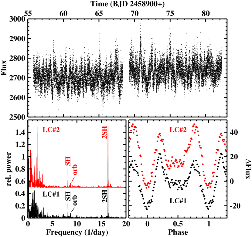
Figure 4: Top: Light curve LC#2 of V592 Cas. Bottom: Power spectra (left) and superhump waveforms (right) derived from light curves LC#1 (black) and LC#2 (red, shifted vertically for clarity).

With one notable exception, apart from overtones and simple arithmetic combinations of the orbital and SH frequencies the power spectra contain no indications of other significant periodicities. In particular, even after applying the same technique as Taylor et al. (1998), i.e., subtracting the pSH variation from the light curve, the present data reveal no trace of a nSH. The exception is a peak at low frequencies (period: 0.53 d) seen in LC#2 which is about as strong as the dominant first overtone of the superhump. It is not present in LC#1. One might therefore suspect it to be due to an accidental alignment of the random low frequency variations of V592 Cas. But this seems not to be the case because it is equally present at very nearly the same frequency in the first and in the second half of the light curve and thus persists at least over its total time base. This periodicity has no obvious relationship to the orbital or the SH period. Its nature remains unclear.

Finally, there is a broad enhancement of power between  65 and 170 d^-1 (8.5 – 22 min) which may explain the 22 min oscillation observed by Kato & Starkey (2002).

3.6 RR Cha: Superhumps and a revision of the WD spin period

Few detailed studies of the quiescent phase of Nova Chamaeleontis 1953 (RR Cha) have been published. Most relevant in the present context is the paper of Woudt & Warner (2002) who discovered eclipses in RR Cha, recurring at a period of 0.1401 d. Moreover, they detected positive as well as negative SHs at periods of 0.14442 d and 0.13529 d, respectively. They also identify a signal in the power spectra of their data corresponding to a period of 32.5 min and suspect RR Cha to be an intermediate polar. Further evidence for this is provided by Rodríguez-Gil & Potter (2003) who observed circular polarization in RR Cha which “appears to be modulated on the spin period of the primary and harmonics of the positive superhump period”.

Due to the faintness of RR Cha, the TESS light curve presents itself to the eye as almost featureless. However, a closer look reveals some interesting properties. The power spectrum of the original data is dominated by a signal at the orbital frequency. The period measured by Woudt & Warner (2002) is based on observations over a time interval of just above 2 d. The TESS light curve with a time base of almost 56 d should therefore permit to increase the accuracy of the orbital period by more than an order of magnitude. Folding the data on the inverse of the orbital frequency derived from the power spectrum yields a representative epoch for the eclipse minimum (Table 2) and the ephemeris

$$T_{\rm ecl}=BJD\,2459363.0160(14)+0.14006(1)\times E$$ (3)

where the error of the epoch is arbitrarily taken to be 1% of the period. The orbital waveform is shown in the upper right frame of Fig. 5. Out of eclipse it is characterized by a symmetrical double hump.

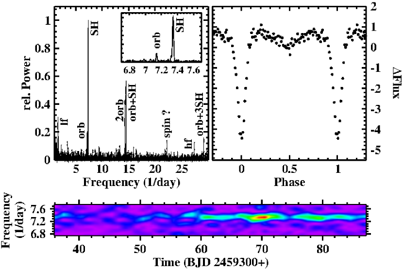
Figure 5: Top Left: Power spectrum of RR Cha. On the scale of the plot the orbital and SH signals are only marginally resolved. Therefore, the insert shows the corresponding frequency range on an expanded scale. To Right: Average waveform of the orbital variations of RR Cha. Bottom: Time resolved power spectrum of the range around the superhump frequency.

The power spectrum of RR Cha, after masking the eclipses, is reproduced in the upper left frame of Fig. 5. It is dominated by a signal at $F_{\rm SH}=7.346(1)$ d^-1 ($P_{\rm SH}=0.13613(2)$ d), just above the orbital frequency. The period is very close to that of the nSH seen by Woudt & Warner (2002). A time resolved power spectrum reveals a significant evolution of the strength of this signal. It starts rather weakly, gains strength in the third quarter of the light curve, and then looses power again, as can be seen in the time resolved power spectrum shown in the lower frame of Fig. 5. The TESS light curve does not contain the pSH detected by Woudt & Warner (2002).

Other signals in the power spectrum can be identified as the first overtone of the orbital frequency and arithmetic combinations of the orbital and the superhump frequencies. However, a peak at 22.215(3) d^-1 cannot be explained in this way. The corresponding period of 64.821(9) min is almost exactly twice the 32.5 min period seen by Woudt & Warner (2002) (with no error margin attached to it) and which they interpret as either the white dwarf spin period or its beat with the orbital period. This can hardly be a coincidence. Depending on the detailed conditions in an individual system the interplay between orbital motion and the white dwarf spin can lead to many different periodic modulations in the light curves (Warner, 1986; Norton et al., 1996). Signals at twice the spin frequency are, for instance, seen in the intermedidate polar AO Psc (see Sects. 3.14). It is therefore conceivable that the period seen by Woudt & Warner (2002) is the first overtone of the spin period (which is not seen in the present TESS data) and that a change in the system configuration leads to a signal at the fundamental period seen now.

Two more apparently significant signals can be detected in the power spectrum, one identified in Fig. 5 as $F_{\rm lf}=1.622(2)$ d^-1 ($P_{\rm lf}=0.6164(7)$ d), the other as $F_{\rm hf}=27.381(3)$ d^-1 ($P_{\rm hf}=0.036522(4)$ d). Neither $P_{\rm lf}=14.8\,{\rm h}$ nor $P_{\rm hf}=52.6\,{\rm min}$ has an obvious relationship to other periods in RR Cha. Thus, their origin remains unexplained.

3.7 V751 Cyg: Nothing new

Patterson et al. (2001) measured a spectroscopic orbital period of 0.1445(1) d for V751 Cyg and found a nSH at 0.13948(7) d. The latter was also seen by Papadaki et al. (2009). The single TESS light curve confirms the continued presence of the superhump at a period of 0.13930(2) d with a very nearly sinusoidal waveform. Fig. 6 shows the light curve, the power spectrum and the superhump waveform. The orbital frequency is marked by a red arrow in the power spectrum, indicating that an orbital signal is notably absent in the light curve. Instead, a clear signal at 1.87 d, i.e., the beat between orbit and superhump, is clearly seen (marked by a red bar in the insert of the lower left frame of Fig. 6). It also appears in the power spectrum of Patterson et al. (2001) The power spectrum does not contain other coherent signals but an enhancement of power between  60 and 75 d^-1 (20 – 24 min), possibly due to QPOs.

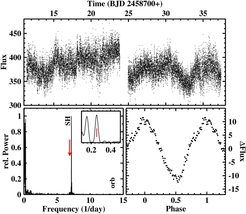
Figure 6: Top: Light curve of V751 Cyg. Bottom left: Power spectrum of V751 Cyg. The red arrow indicates the frequency of the orbital period which is not detectable in the light curve. The insert shows the low frequency part the power spectrum where the beat frequency between orbital and the superhump signals is marked by a red bar. Bottom right: Waveform of the superhump modulation.

3.8 V1974 Cyg: Superhumps and a 1.3 d variation

V1974 Cyg (Nova Cygni 1992) exhibits two distinct photometric periodicities. The first one, at 0.0812585(5) d (DeYoung & Schmidt, 1993; Retter et al., 1997), is considered to be orbital. A second slightly variable period close to 0.0850 d (Semeniuk et al., 1994, 1995; Retter et al., 1997) can be interpreted as a positive superhump. A third periodicity of 0.08304 d was seen in 1994 by Retter et al. (1997) but did not show up in 1995.

The two available TESS light curves, separated by two years, confirm the presence of the orbital signal at 0.08127(2) d while the superhump signal yields slightly different periods of 0.08504(2) and 0.08525(2) d in LC#1 and LC#2 (Fig. 7). Both signals are of comparable strength in the power spectra. Additionally, the power spectrum of LC#2 contains another peak, marked with a question mark in the figure, which is almost as strong as the superhump signal. It corresponds to a period of 1.281(7) d. Note that this is not the beat period between the orbital and superhump modulations. Its origin remains unclear but is reminiscent of the 0.53 d period seen in LC#2 of V592 Cas (Sect. 3.5). The 0.083 d period reported by Retter et al. (1997) cannot be deteced in the TESS light curves.

It is noteworthy, however, that in addition to the superhump Semeniuk et al. (1994) found a period of 3.75 d in their data. Although they do not quote error limits, their fig. 7 suggests that this period is compatible with twice the beat between the orbital and the superhump periods (1.84 d) (see also Semeniuk et al., 1995), similar to what has been seen by Bruch & Cook (2018) in V603 Aql.

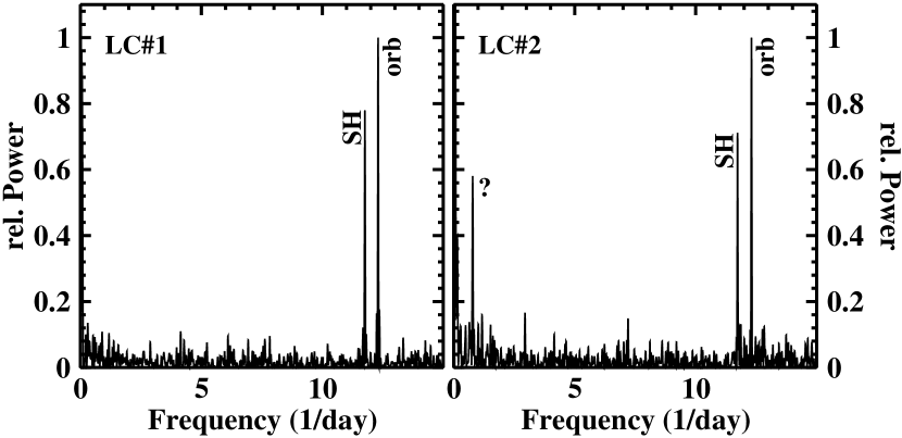
Figure 7: Power spectra of the two TESS light curves of V1974 Cyg.

3.9 BB Dor: Four periods, but not the orbital one

BB Dor (= EC 05287-5847) was identified as a cataclysmic variable by Chen et al. (2001). Their tentative classification as a VY Scl type star was confirmed by Rodríguez-Gil et al. (2012). The latter authors observed long term variations with a period of 36.43 d as well as a spectroscopic orbital period of 0.154095(30) d. A period of 0.14923(7) d – observed and thought to be orbital by Patterson et al. (2005) – would then be due to a nSH, while a weaker signal at 0.1633 d indicates a pSH. Another still much weaker signal in their power spectrum has a frequency of 12.833 d^-1, very nearly the sum of the two superhump frequencies.

TESS observed BB Dor in no less than 20 sectors. The star remained in a stable high state all the time. The individual light curves can be combined into two long ones, both with baselines of almost a year (there is a gap of 27 d in the second light curve). LC#1 is shown in the upper frame of Fig. 8. The middle frame contains the light curve of sector 12. Periodic or semi-periodic variations are obvious on three different time scales: some tens of days, just over one day, and a fraction of a day. Predicted times of maxima for the first two of these, based on a formal period measurement (see below) are marked by red dots on top of the light curves in the figure.

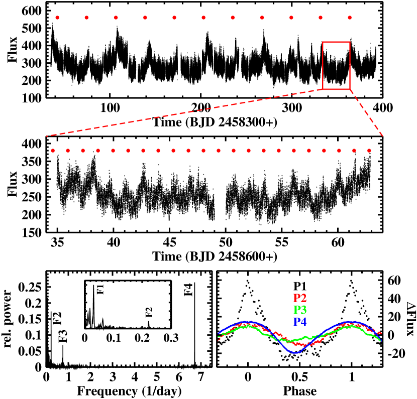
Figure 8: Top: Light curve LC#1 of BB Dor. Middle: Light curve of TESS sector 12. The red dots above the light curves mark predicted times of maxima of variations with a period/quasi-period of 32.15 d (top) and 1.35 d (middle). Bottom left: Power spectrum of LC#1. The insert contains an expanded view of the low frequency range. Bottom right: LC#1 folded on the four independent periods identified in the light curves (after subracting variations on longer time scales).

The power spectrum LC#1 is reproduced in the lower left frame of Fig. 8. That of LC#2 is practically identical. Four independent signals can be identified. The corresponding frequencies $F_{1}$ - $F_{4}$ are marked in the figures and listed together with the corresponding periods in Table 3. On a low power level (not resolved in the figure) several more significant peaks appear, but they all occur at frequencies equal to simple arithmetic combinations of the main signals and are therefore not independent. $P_{1}$ varies significantly, $P_{2}$ – $P_{4}$ only slightly between LC#1 and LC#2. In fact, in the power spectrum of the combined data the corresponding peaks split up into two. Therefore, values derived from both light curves are listed in the table.

The bottom right frame of Fig. 8, finally, shows LC#1 folded on the four periods, after variations on appropriate longer time scales have been subtracted in the case of $P_{2}-P_{4}$. The waveforms derived from LC#2 are not significantly different.

Table 3: Independent frequencies and their corresponding periods identified in the light curves of BB Dor.

	LC	Frequency (d-1)	Period (d)
$F_{1}$	LC#1	0.0311 (2)	32.1 (2)
	LC#2	0.0267 (2)	37.5 (3)
$F_{2}$	LC#1	0.2225 (2)	4.495 (3)
	LC#2	0.2231 (1)	4.483 (3)
$F_{3}$	LC#1	0.7549 (2)	1.3247 (3)
	LC#2	0.7533 (2)	1.3227 (4)
$F_{4}$	LC#1	6.71402 (2)	0.1489422 (4)
	LC#2	6.71454 (3)	0.1489305 (6)

The slight differences in time between the brightness peaks and the red dots in the upper frame of Fig. 8 and the significantly different periods found in LC#1 and LC#2 indicate that the $P_{1}$ variations are not strictly periodic. Nevertheless, they can clearly be identified with the quasi-periodic brightenings observed by Rodríguez-Gil et al. (2012). The different periods in the two TESS light curves [embracing the period of Rodríguez-Gil et al. (2012)], separated by a year, indicates that they are not caused by a stable clock in BB Dor. However, their persistence over more than 14 yr tells us that this is not just a transient phenomenon. Rodríguez-Gil et al. (2012) speculate that these variations are due to mass transfer variation caused by migrating star spots on the secondary star or stunted outbursts. But it is then not obvious why the brightenings occur with a reasonable well defined periodicity. The convex shape of the light between maxima suggests a gradual build-up and subsequent decay of the (so far unknown) process responsible for the modulations.

$P_{4}$ is very close to the main photometric period seen by Patterson et al. (2005) and which is interpreted by Rodríguez-Gil et al. (2012) as due to a nSH. One of the fainter power spectrum peaks mentioned above (better defined in LC#2 than in LC#1) has a frequency of 6.4918 (5) d^-1, which on the one hand is within the error margin of the spectroscopic orbital period and on the other hand is almost identical to $F_{4}-F_{2}$. Thus, $P_{4}$ can indeed be identified with a nSH period, and $P_{2}$ is correspondingly the nodal precession period of a warped accretion disk.

What about $P_{3}$? Could it be the apsidal precession period of an excentric disk? In that case the expected frequency of a pSH would be $F_{3}+F_{\rm orb}=7.245\ (1)$ d^-1. The closest marginally significant peak in the power spectrum of LC#1 is at 7.2558(6) d^-1. The period difference between the orbital and the superhump periods would then be three times as large for the positive than for the negative superhump. While not impossible, this is significantly more than the canonical difference of a factor of two. It may also be questioned why the superhump signal is then so much fainter than that due to the apsidal disk motion. An alternative, but equally unsatisfactory hypothesis is an interplay between $P_{1}$ and $P_{2}$. Is it a coincidence that in both light curves $3\left(F_{1}+F_{2}\right)=F_{3}$ within the formal $1\sigma$ error margin? As long as the origin of $P_{1}$ remains unknown it is difficult even to speculate about a reason for such an interplay.

The long light curves permit a closer look at the temporal development of the periodic signals. The time resolved power spectrum of LC#2, in the frequency range of the nSH and of $F_{3}$, constructed using a sliding window with a width of 10 d, is shown in the middle and lower frames, respectively, of Fig. 9, with the light curve shown in the upper frame. The corresponding power spectrum of LC#1 is very similar. The superhump signal itself does not vary significantly with time. But it is flanked symmetrically on both sides (stronger at frequencies lower than the SH frequency) by structures modulated with the long period ($P_{1}$) variations. Their frequency difference with respect to the SH frequency is equal to the frequency of the $F_{3}$ signal in the lower frame of the figure. $F_{3}$ is approximate constant during “quiescent” phases, subsides at the onset of the brightenings and reappears at a lower frequency during their maxima.

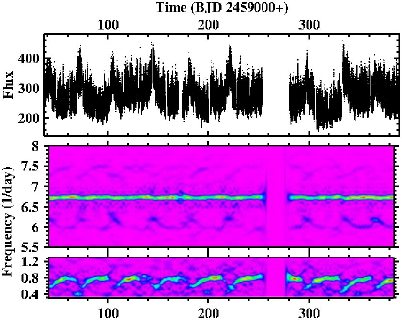
Figure 9: Top: Light curve LC#2 of BB Dor. Middle: Time resolved power spectrum of the light curve in a small range around the nSH frequency. Bottom: The same for a frequency range around $F_{3}$.

As a final remark on BB Dor, I note that the power spectra of the TESS light curves contain an excess of power between 30 and 100 d^-1, encompassing the range in which Chen et al. (2001) observed QPOs.

The complex variability of BB Dra disclosed by the long TESS light curves certainly deserves a more detailed investigation and interpretation. But this is beyond the scope of the present paper and must await a specific study.

3.10 BH Lyn: Positive Superhumps and QPOs

BH Lyn was discovered as PG 0818+513 in the Palomar-Green survey (Green et al., 1986). The system is eclipsing and thus makes it easy to determine a reliable orbital period which has been derived many times in the past. The most precise value of 0.155875577(14) d was measured by Stanishev et al. (2006). They also noted the presence of variations at a slightly smaller period of 0.1450(65) d which they interpret as a nSH. A similar variation at 0.1490(011) d was also seen by Patterson (1999). Additionally, Stanishev et al. (2006) observe the presence of a signal close to 32 d^-1 in the power spectra of most of their light curves which they attribute to QPOs.

The two available TESS light curves of BH Lyn exhibit irregular variations on time scales of a few days. Apart from the primary eclipse the orbital waveform exhibits a clear secondary eclipse. More interesting, however, are the power spectra (after masking the primary eclipses). On the left side of Fig. 10 the power spectrum of LC#1 is reproduced, concentrating on a frequency range of $\pm 2.5$ d^-1 around the orbital frequency and its first, second and third overtone. The peak caused by the orbital variations is highlighted in red. On the right side of the figure the time resolved power spectra in the same frequency range are shown, based on a sliding window with a widths of four days (thus, structures separated by less than four days are not independent). The general apparence of the power spectra of LC#2 is very similar.

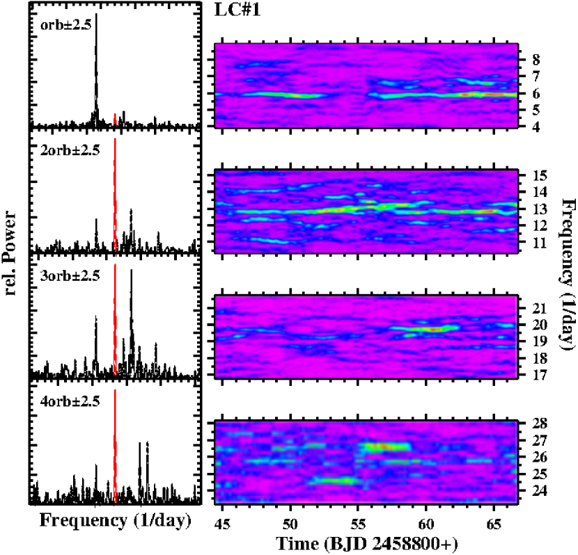
Figure 10: Left: Power spectra of LC#1 of BH Lyn in four narrow frequency ranges of $\pm$2.5 d^-1 around the orbital frequency and its first, second and third overtone (highlighted in red). Right: Time resolved power spectra of the same frequency range, using a sliding window with a width of four days.

While in none of the power spectra a significant peak is detected at a frequency close to that corresponding to the nSHs seen by Patterson (1999) and Stanishev et al. (2006), the dominant signal in the upper frames of the figure has a frequency just below the orbital frequency. The time resolved power spectrum shows that, albeit exhibiting some modulation in its strength, this signal is persistent over the whole extend of the light curve. It indicates thus the presence of a pSH with a period of 0.17059(5) d in LC#1. A similar persistent pSH is also seen in LC#2, but at a significantly shorter period of 0.16484(4) d. The period excess $\epsilon=\left(P_{\rm SH}-P_{\rm orb}\right)/P_{\rm orb}$ thus drops from 0.094 in LC#1 to 0.058 in LC#2. While it is known that superhump periods can change over time, such a large difference of $\epsilon$ at different epochs is unusual.

Apart from the orbital and SH signals the power spectra contain a multitude of peaks in narrow frequency ranges around the orbital frequency and its overtones. They appear less clearly also at higher overtones than shown in Fig. 10 [note that the QPOs claimed by Stanishev et al. (2006) at 32 d^-1 are very close to the forth overtone of the orbital frequency]. No simple relation between them is apparent, meaning that they are independent from each other. The time resolved power spectra reveal that they can appear for considerable time intervals with varying strength and frequency changes. These are characteristics of QPOs. Their concentration around the orbital frequency and its overtones is noteworthy. While not as extreme, this behaviour is reminiscent of similar properties observed in the old nova CP Pup (see Paper I) and BZ Cam (Sect. 3.4).

Finally, representative eclipse epochs of BH Lyn are listed in Table 2 for future reference.

3.11 BK Lyn: Positive superhump, yes, but no negative one

BK Lyn (=PG 0917+342) is a novalike variable with some curious peculiarities. At an orbital period of 0.07498(4) d (Ringwald et al., 1996) it is one of very few (non-magnetic) novalike variables below the CV period gap. In a never before seen transition, in 2005 BK Lyn morphed into a ER UMa star (Patterson et al., 2013), i.e., an SU UMa star with many normal outbursts in quick succession and a very short supercycle. However, in 2014 the system returned to the more stable high brightness state of a NL, as is evident from the AAVSO long term light curve. Superhumps were first seen in BK Lyn by Howell et al. (1991) but misinterpreted as orbital variations. Skillman & Patterson (1993) then correctly identified a 113.1 min modulation with a slightly varying period as a pSH which was later confirmed by Misselt & Shafter (1995). In a more extensive photometric study Patterson et al. (2013), in addition to pSHs, also detected their negative counterparts in some observing seasons. Finally, Yang et al. (2017) claim the presence of a long term period of 42.05(1) d in BK Lyn.

The only TESS light curve available (upper frame of Fig. 11) shows a clear modulation on the time scale of about 1.5 d superposed on a longer period variation. The latter is well fit by a sine wave with a period of 17.29(3) d (the red line in the figure). But since the light curve covers only just about 1.5 cycles it is by no means clear that this modulation is, in fact, periodic and persistent. The origin of the more rapid variations becomes immediately clear looking at the power spectrum in the lower left frame of Fig. 11 which is dominated by a strong signal at $F_{\rm SH}=12.7096(3)$ d^-1 ($P_{\rm SH}=0.078681(2)$ d). It is evidently due to the pSH observed on previous occasions and now has a slightly longer period. A much fainter signal is present at a higher frequency of $F_{\rm orb}=13.344(2)$ d^-1 ($P_{\rm orb}=0.074942(9)$ d). Within the error quoted by Ringwald et al. (1996) this period is identical to the spectroscopic orbital period but has a higher precision. Another signal appears at a low frequency of $F_{\rm b}=0.633(1)$ d^-1 ($P_{\rm b}=1.579(3)$ d). Within the error margins this is the difference between $F_{\rm orb}$ and $F_{\rm SH}$ and thus the period of the apsidal motion of an eccentric disk in the canonical interpretation of positive superhumps. It explains the shorter time scale modulations seen in the light curve. At higher frequencies signals at simple arithmetic combinations of $F_{\rm orb}$ and $F_{\rm SH}$ appear, but the data contain no trace of the nSH seen by Patterson et al. (2013).

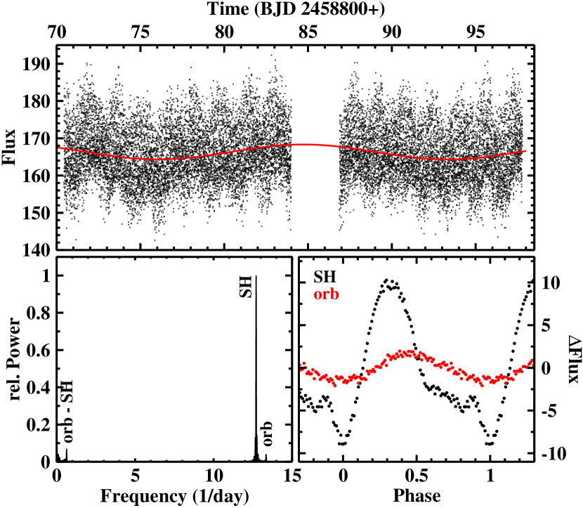
Figure 11: Top: Light curve of BK Lyn. The red graph represents a least squares sine fit with a period of 17.29 d. Bottom: Power spectrum of BK Lyn (left) and waveforms of the superhump and orbital modulations (right).

The waveform of the superhump variations (in black, together with the unconspicuous quasi-sinusoidal orbital waveform in red) is shown in the lower right frame of Fig. 11. Over the years the superhump shape varies. In the TESS data it comprises only the first have of the cycle. The second half is characterized by an only slighly declining level in the phase range 0.55 – 0.85 before dropping to the minimum at phase 0. In Patterson et al. (2013) (their figure 3) the waveform is clearly double humped, while Skillman & Patterson (1993) observed an almost sinusoidal superhump (their figure 6).

3.12 AH Men: Shallow eclipses and a strong negative superhump

Buckley et al. (1993) published the first encompassing photometric study of AH Men (1H05551-819). Apart from QPO-like variations in the range of 600 - 2400 s they detected the presence of a quasi-sinusoidal modulation at 0.1392202(9) d. Radial velocities measurements confirm that this variation “occurs at, or very near to, the orbital period”. This, however, is at odds with later observations of Patterson (1995) who noted the continuous presence of a signal at 0.1229934 (6)d. While in 1995 AH Men did not exhibit other coherent variations, between December 1993 and February 1994 Patterson saw strong variations at 0.127208 d (which he considers orbital), 0.12300 d, 0.062517 d and 3.7 d, as well as oscillations in the range of 17 – 22 min. In a later paper Patterson (1998) mentions a superhump period of 0.1385(2) d. Should this [and the period seen by Buckley et al. (1993)] be due to a pSH, while the 0.12300 d period points at a nSH?

The upper frame of Fig. 12 shows one of the five available TESS light curves (LC#5). It is dominated by regular variations which, as we will see, are due to the beat between the orbital and a nSH period. While this signal shows up in the power spectra of all light curves it is obvious to the eye only in LC#3 and later. Apart from this periodicity the power spectrum of LC#5 (lower left frame of the figure) just as that of all other light curves is dominated by a strong peak close to 8.09 d^-1 and some much fainter satellite lines, as shown in the lower left frame of the figure and on an expanded scale in the left insert. I interpret the strong $F_{\rm SH}=8.09$ d^-1 signal as being due to a negative superhump and a smaller peak at $F_{\rm orb}=7.86$ d^-1 as orbital. Other signals are related to the beat between them. At higher frequencies another group of signals appears (right insert), the strongest occurring at $2F_{\rm orb}=15.72361(8)$. At still higher frequencies additional peaks are seen which can all be interpreted as linear combinations of $F_{\rm orb}$ and $F_{\rm SH}$.

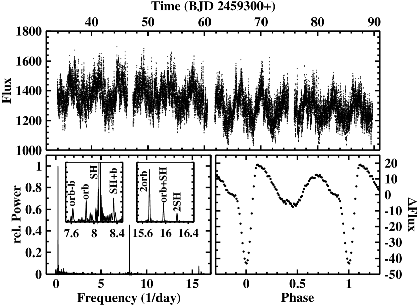
Figure 12: Top: Part of LC#5 of AH Men. Bottom left: Power spectrum of the light curve. The inserts contain small frequency intervals of this power spectrum on an expanded vertical scale. Here, “b” stands for the beat frequency between the orbital and superhump signals. Bottom right: Orbital waveform of AH Men (average of all light curves).

Why do I consider $F_{\rm orb}$ to be orbital in nature? This becomes obvious when folding the light curves on the corresponding period. The average of all folded light curves is shown in the lower right frame of Fig. 12. It clearly reveals a double-humped structure and a rather shallow eclipse. This waveform explains why the first overtone of $F_{\rm orb}$ in the power spectra is so much stronger than the fundamental frequency. On the other hand, folding the light curves on $1/F_{\rm SH}$ yield a nearly sinusoidal waveform, albeit with a much larger amplitude. Based on all light curves (eclipse timings are listed in Table 2), the following ephemeris for the eclipse minimum is derived:

$$T_{\rm min}=BJD2458340.0869(2)+0.12719550(5)\times E$$

Although rather stable, the period of the superhump varies slightly. The corresponding values measured in the individual light curves are: 0.12364(3) (LC#1), 0.12383(3) (LC#2), 0.123485(5) (LC#3), 0.12337(2) (LC#4) and 0.123446(6) (LC#5).

3.13 RR Pic: Only transient superhumps

RR Pic is a well studied old nova. The orbital period reveals itself in the form of a clear and persistent hump first seen by van Houten (1966) and ever since. The most precise value of 0.145025959 d was derived by Fuentes-Morales et al. (2018). They also saw pSHs with a period of 0.1577 in 2007. Schmidtobreick et al. (2008) report another superhump instance in 2005 with the same period and which went along with a signal at the beat between the SH and orbital periods.

The numerous sectorial data sets of RR Pic observed by TESS can be combined into 5 contiguous light curves, two of which encompass about 8 months. The orbital signal is outstanding in the respective power spectra, but no trace of a superhump is visible, even after carefully subtracting the average orbital waveform from the data (Fig. 1c). It is, however, remarkable that the waveform is extremely stable [and quite similar to the one shown in fig. 3 of Schmidtobreick et al. (2008)] over the almost 3 years spanned by the data. Even small details are faithfully repeated in the waveforms derived from the individual light curves.

Schmidtobreick et al. (2008) and Fuentes-Morales et al. (2018) analyzed light curves of RR Pic from 11 observing seasons and saw superhumps only twice. Adding to this the TESS data without SHs (over a total time base of $\approx$3 yr) makes it clear that superhumps in this system are only rare and transient events.

3.14 AO Psc: No confirmation of superhumps

The optical light curve of the well known intermediate polar AO Psc is dominated by the orbital period at 0.1495 d and the orbital side band of the white dwarf spin period at 14.31 min (Patterson & Price, 1981; Motch & Pakull, 1981). SHs in AO Psc with a period of 0.149627 d are only mentioned briefly by Patterson (2001) who referred details to a publication in preparation which, however, never appeared.

The power spectrum of the single TESS light curves contains strong signals at the orbital frequency $F_{\rm orb}$, the orbital sideband of the white dwarf spin frequency $F_{\rm spin}-F_{\rm orb}$, and weaker signals at $2F_{\rm orb}$, $F_{\rm spin}$, $F_{\rm spin}-2F_{\rm orb}$, $2F_{\rm spin}$ and $2F_{\rm spin}-2F_{\rm orb}$. But there are no indications of superhumps (Fig. 1d).

3.15 AY Psc: No superhumps, but an increasing orbital period

In contrast to the other objects in this study, AY Psc is a dwarf nova. It belongs to the Z Cam stars (Mercado & Honeycutt, 2002), i.e., those dwarf novae which occasionally remain in a standstill. The TESS light curve, observed in subsequent time intervals in two sectors and covering 51 days, is rather stable and does not contain the usual alternations between outbursts and quiescent phases with a quasi-period of 18.3 d (Han et al., 2017). It may therefore be concluded that the system was in a standstill during the entire observing period. During such phases the accretion disk is expected to be be in a hot state similar to those of NLs and old novae. Therefore, I include AY Psc in this study.

AY Psc is an eclipsing system as first noticed by Szkody et al. (1989). Orbital ephemeris were provided by Diaz & Steiner (1990) and later refined by Gülsecen et al. (2009) and Han et al. (2017). Gülsecen et al. (2009) reported the presence of nSHs with a slightly changing period between 0.2057 and 0.2073 d during three observing missions in 2003, 2004 and 2005. The total amplitude of the light variations of AY Psc in each of these missions was about 2.25 mag which is similar to its average outburst amplitude (Han et al., 2017). Thus, the system was observed during a period of normal dwarf nova activity. Gülsecen et al. (2009) did not investigate a dependence of the superhump properties on the phase of the outburst cycle.

The power spectrum of the TESS light curve (after masking the eclipses) does not confirm the presence of SHs Fig 1e). The only significant signals are at the orbital frequency and its overtones. Thus, if nSHs occur during the normal activity cycle of AY Psc, they subsided at least during the prolonged standstill covered by TESS.

The many eclipses in the TESS light curve permit, together with data taken from the literature, an improvement of the orbital period of AY Psc. Representative eclipse timings for the light curves observed in the two sectors covered by TESS are listed in Table 2. These, together with the eclipse timings listed by Diaz & Steiner (1990) and Han et al. (2017), including also the eclipse epoch taken from the ephemeris of Gülsecen et al. (2009) (unfortunately, they do not list individual eclipse timings), assigning a weight of 1 to the literature timings and 10 to the representative TESS eclipse epochs, yield the linear ephemeris:

$$T_{\rm min}=BJD\,2447623.3460(2)+0.217320654(4)\times E$$ (4)

Here, the errors are the formal fits error of the linear fit to the cycle number – eclipse epoch relation.

The $O-C$ diagram with respect to the linear ephemeris is shown in the left frame of Fig. 13 where the red graph is a fit of a 2^nd order polynomial to the data. It suggests that quadratic ephemeris provide a better description of the eclipse timings:

$$T_{\rm min} = BJD\,2447623.34640(6)$$

$$+0.217320452(1)\times E$$

$$+3.69(2)\,10^{-12}\times E^{2}$$

The period increases thus currently at a rate of $\dot{P}=3.40(3)\times 10^{-11}$. The relative period increase is $\dot{P}/P=5.71(4)\times 10^{-8}$ yr^-1.

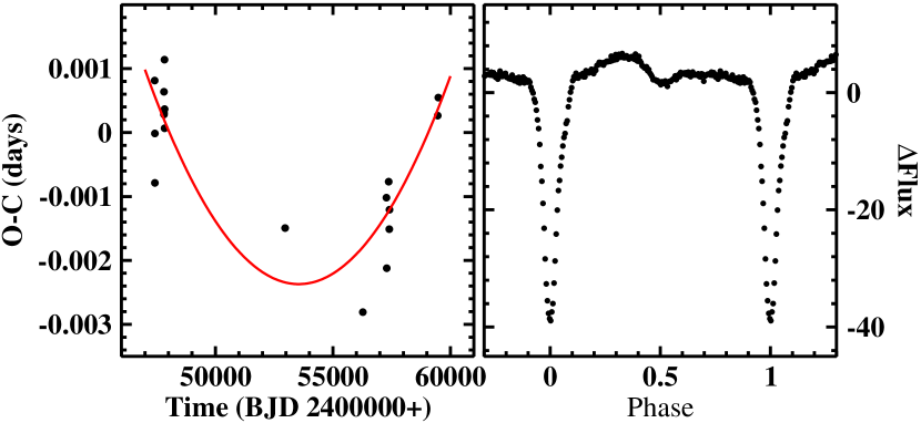
Figure 13: Left: $O-C$ diagram of eclipse timings of AY Psc with respect to linear ephemeris (Eq. 4). The red graph is a least squares fit of a 2^nd order polynomial to the data. Right: Orbital waveform of AY Psc during standstill.

The light curve, folded on the orbital period, yields the waveform shown in the right frame of Fig. 13. Apart from the primay eclipse a secondary eclipse occurs at phase 0.5. It is preceded by a hump. No hump is apparent at the phases before the primary eclipse, in contrast to what is often seen in other eclipsing CVs and is attributed to enhanced emission from a bright spot. The waveform is thus different from that observed by Gülsecen et al. (2009) in white light (see their fig. 3), but this may at least in part be due to the different passband of TESS.

3.16 V348 Pup: Superhumps confirmed

At an orbital period of 0.101838931(14) d (Rolfe et al., 2000), V348 Pup is an eclipsing novalike variable right at the centre of the CV period gap. Photometric variations with a period slightly different from the orbital one made Tuohy et al. (1990) suspect the star to be what would nowadays be considered an asynchronous polar; a notion which could neither be confirmed no rejected in pointed X-ray observations by Rosen et al. (1994), while Froning et al. (2003) found no evidence for a magnetic nature. Instead, Rolfe et al. (2000) reported SHs with a slightly variable period in V348 Pup in 1991, 1993 and 1995 which, however, were not seen when Saito & Baptista (2016) observed the star at a later epoch.

The light curve of V348 Pup, combining data from two TESS sectors, is shown in the upper frame of Fig. 14. The strong out-of-eclipse variations have a period of 1.797(1) d and immediately suggest to be due to the beat between the orbital and a SH period and thus the precession period of an accretion disk. This is confirmed by the power spectrum (lower left frame of the figure) which, apart from the dominating signal at the beat frequency, contains a peak at the orbital frequency $F_{\rm orb}$ and a strong signal at $F_{\rm SH}=9.2626(8)\,{\rm d}^{-1}$ ($P_{\rm SH}=0.107961(9)$ d). The period of the latter lies within the range of SH periods observed by Rolfe et al. (2000), leaving no doubt that it is due to a positive superhump. Other signals and a multitude of peaks at frequencies beyond the range shown in the figure can all be expressed as simple arithmetic combinations of $F_{\rm orb}$ and $F_{\rm SH}$. The waveform of the superhump is significantly structured as seen in the lower right frame of Fig. 14.

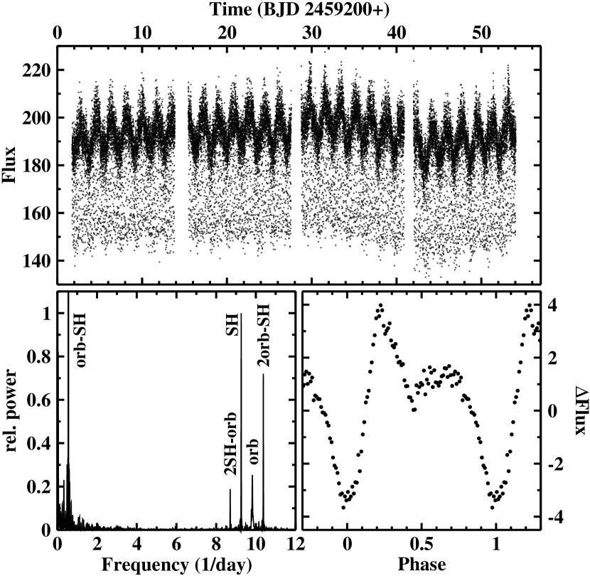
Figure 14: Top: Light curve of V348 Pup. Bottom: Power spectrum (left) and superhump waveform (right).

Investigating all available eclipse timings available at the time, Dai et al. (2010) concluded that the orbital period of V348 Pup is currently increasing. Average eclipse epochs derived from the two TESS sector data (Table 2) and 9 additional epochs measured in archival light curves retrieved from the LNA Data Bank (Table A2) permit to extend the total time base. I confirm the period increase and derive quadratic ephemeris for V348 Pup which are very similar to those quoted by Dai et al. (2010):

$$T_{\rm min} = BJD\,2448591.668(1)$$

$$+0.1018389(2)\times E$$

$$+2.6(1.7)\,10^{-13}\times E^{2}$$

3.17 RW Tri: no superhumps in TESS data

RW Tri is a deeply eclipsing novalike variable of the UX UMa type. Low amplitude ($\approx 0.5$ mag) oscillations on time scales of some tens of days have been observed by Honeycutt et al. (1994), Honeycutt (2001), and even more clearly by Bruch (2020). Apart from this the system is relatively stable as is corroborated by the long term AAVSO light curve. Smak (2019) reports nSHs with a period of 0.2203 d in his observations obtained in 1984 and possibly in 1957. They were, however, not present in 2015 – 2016 (Bruch, 2020). The more extensive continuous TESS data permit an additional verfication of Smak’s claim of superhumps in RW Tri.

A single TESS light curve of the system is available (upper frame of Fig. 15). Over its 24 d time base a gradual rise and subsequent decline in brightness occurs which is roughly compatible with the oscillations mentioned above. The flux level at the bottom of the eclipses follows these variations. This means that the responsible light source is not eclipsed.

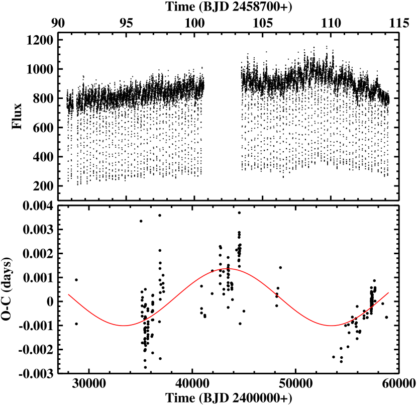
Figure 15: Top: TESS light curve of RW Tri. Bottom: $O-C$ diagram of eclipse timings of RW Tri with respect to linear ephemeris (Eq. 7). The red graph is a least squares sine fit.

The power spectrum does not contain significant signals at frequencies other than the orbital frequency and its overtones (Fig. 1f). Thus, at least during the epoch of the TESS observations no superhumps were excited in RW Tri.

As in the case of UU Aqr the last update of the orbital period of RW Tri occurred decades ago (Robinson et al., 1991). I retrieved numerous light curves from the AAVSO archives observed between 2005 and 2018 and measured 95 additional eclipse epochs in the same way as was done for UU Aqr and V348 Pup. The results are listed in Table A3. They were used together with the representative eclipse epoch derived from the TESS light curve (see Table 2), which got 10 times the weight of the individual eclipses, and those listed by Mandel (1965), Africano et al. (1978) and Robinson et al. (1991) to recalculate orbital ephemeris for RW Tri:

$$T_{\rm min}=BJD\,2453672.6246(4)+0.231883245(6)\times E$$ (7)

Not surprisingly, the orbital period is very close to the value quoted by Robinson et al. (1991). As in many other CVs the $O-C$ curve, now covering over 80 yr (albeit only sparsely covered during the first $\sim$15 yr), exhibits systematic variation on the time scale of years, indicating small fluctuations of the orbital period which cannot be attributed to the secular evolution of the system. These variations are, however, much more gradual in RW Tri than the very rapid period changes in UX UMa (see Sect. 3.18). With some good will one might even suspect a cyclic variation with a period of 55 yr (red curve in the figure), but covering only just about one cycle I am reluctant to claim it to be persistent.

3.18 UX UMa: Superhumps remain to be isolated events

UX UMa is the prototype of novalike variables, in particular of those system which, in contrast to VY Scl stars, have never been observed to go into a low state. As the prototype of its class and the brightest eclipsing novalike variable, UX UMa has been extensively studied in the past (see Neustroev et al., 2011, for a summary of previous observations). The orbital period was last refined by Baptista et al. (1995). In extensive photometric observations during the 2015 observing season de Miguel et al. (2016) found a modulation with a period of 3.680 d in the light curve of UX UMa which they interpret as being due to a retrograde precession of the accretion disk. An associated nSH at the beat period of the precession and the orbit is also seen. Bruch (2020) confirmed this behaviour but also noted that it was restricted to that particular season and did not repeat itself in previous or following years.

Is there any trace of the unusual behaviour observed in 2015 to be found in the TESS observations taken in 2019, Aug-Oct and 2020, Feb-Apr? No, there is not. The power spectra of the two TESS light curves do not contain any significant signal other than the orbital one and its overtones (Fig. 1g). The orbital waveform (left frame of Fig. 16) is characterized – apart from the primary eclipse – by a single hump, interrupted by the secondary eclipse which gives the hump the structure of two separate “horns”. The primary eclipse egress exhibits a clear change of gradient, i.e., the typical sign of a retarded egress of a hot spot. The flux level just after eclipse egress is considerably lower than just before ingress. This waveform is different from that normally observed at shorter wavelengths (see fig. 20 of Bruch, 2020). A comparison of the waveforms out of eclipse resulting from LC#1 (black) and LC#2 (red) is shown in the right frame of the figure. Only slight variations occur in the 6 months between the light curves.

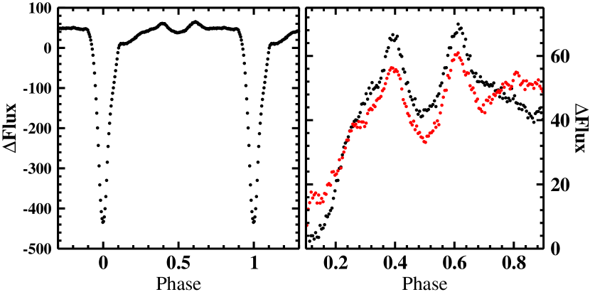
Figure 16: Left: Orbital waveform of UX UMa (average of LC#1 and LC#2). Right: The same on an expanded vertical scale, restriced to out-of-eclipse phases and shown separately for LC#1 (black) and LC#2 (red).

Just as for UU Aqr and RW Tri, the orbital period of UX UMa was last refined almost 30 yr ago (Baptista et al., 1995). Again, I took advantage of light curves observed between 1999 and 2022 found in the AAVSO archives, as well as of some unpublished light curves taken between 1977 and 1992, provided by R.E. Nather and E.L.. Robinson (private communication). They yielded no less than 291 useful additional eclipse epochs (Table A4). Representative eclipse epochs derived from the TESS light curves are listed in Table 2.

Combining the new eclipse timings with those listed by Nather & Robinson (1974), Africano & Wilson (1976), Kukarkin (1977), Quigley & Africano (1978), Rubenstein et al. (1991), Rutten et al. (1992) and Baptista et al. (1995) (as usual assigning weight 10 to the TESS eclipse epochs and 1 to all others) yielded the following revised orbital ephemeris for UX UMa:

$$T_{\rm min}=BJD\,2451319.779(3)+0.19667127(7)\times E$$ (8)

It turns out that within the $1\sigma$ error the period is identical to the one derived by Baptista et al. (1995). Indeed, in spite of the much longer time base the formal error increased. This is explained by the $O-C$ diagram, reproduced in the left frame of Fig. 17, which reveals an increased non-random scatter of the data points in recent years.

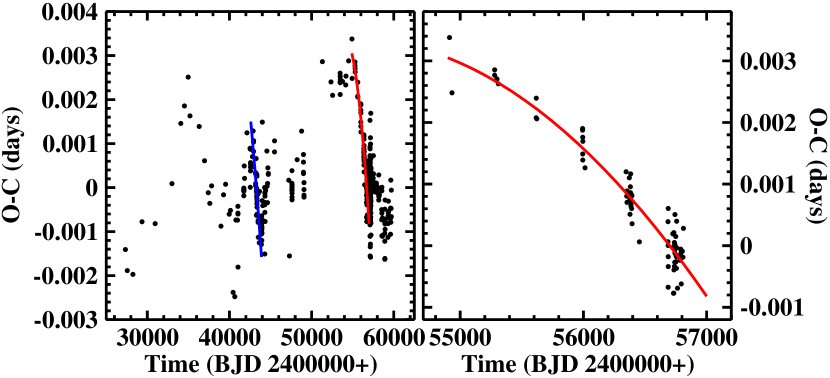
Figure 17: Left: $O-C$ diagram of the eclipses in UX UMa. The blue and red lines mark intervals of particularly strong gradients. Right: Detail of the $O-C$ diagram corresponding to the interval marked by the red line in the left frame, together the least squares parabolic fit to the data.

In the early years, a 29 yr cyclic variation of the orbital period of UX UMa was first suspected by Mandel (1965) and further discussed by Nather & Robinson (1974) and Africano & Wilson (1976), but then called into question by Kukarkin (1977) and Quigley & Africano (1978). Regarding the $O-C$ diagram in fig. 5 of Baptista et al. (1995) this hypothesis can clearly be rejected. This is impressively confirmed by the present results (Fig. 17) which extends the time base by about a factor of 2. The $O-C$ diagram indicates non-periodic but systematic variations of the the orbital period on widely varying time scales. The most rapid $O-C$ (and consequently period) changes are highlighted by blue and red lines in the figure which have very nearly the same gradient. The right frame of Fig. 17 contains an enlarged version of one of these $O-C$ diagram sections. The red line represents a least squares 2^nd order polynomial fit to the data which yields a period change of $\dot{P}=-1.97\times 10^{-10}$. This corresponds to a time scale for the period decrease as short as $P/\dot{P}=2.73\times 10^{6}$ yr.

On secular time scales the periods of cataclysmic variable are expected to decrease due to angular momentum loss of the system via magnetic breaking and gravitational radiation. Such variations are monotonic and occur on vastly longer time scales than observed here. Period variations on time scales of years and with changing sign are not uncommon in CVs. If they are cyclic they are often explained by the presence of a third body in the system (a hypothesis more often than not disproved by additional observations). Alternatively, the Applegate mechanism (Applegate, 1992) is frequently invoked with mixed success. However, it appears fair to say that so far no generally excepted idea to explain the often erratic period variations has been put forward.

3.19 DW UMa: A positive, yes, but no negative superhump

The eclipsing system DW UMa has been subjected to many photometric studies which revealed the presence of positive and negative superhumps. The most extensive investigation was performed by Boyd et al. (2017) who also cite references to other relevant papers. The orbital period is 0.1366065324(7) d. SHs were observed with slightly varying periods around 0.133 d (nSH) and 0.145 d (pSH). The beat period between the orbit and the superhumps is also clearly seen.

The latter feature is impressively confirmed in the two TESS light curves, the first of which is reproduced in the upper frame of Fig. 18. The power spectra (after masking the eclipses) basically confirm the earlier results with the noticeable exception that no trace of a nSH is present. Without assessing their formal significance I identified no less than 40 (LC#1) and 35 (LC#2) peaks up to the Nyquist frequency which appear to stand out above the surrounding “continuum”. All except 3 (LC#1) and 5 (LC#2) can be explained as $nF_{\rm orb}+mF_{\rm b}$ where $F_{\rm b}=F_{\rm orb}-F_{\rm SH}$ and $n$ and $m$ are integer values in the range $1\leq n\leq 46$ and $-4\leq m\leq 2$. The pSHs have significantly different periods of 0.14387(2) d (LC#1) and 0.14479(3) d (LC#2) in the two light curves separated by $\approx$2 yr. The orbital (eclipses masked) and superhump waveforms are shown in the lower frames of Fig. 18. Large (orbital) and moderate (superhump) differences between LC#1 and LC#2 are evident. For future reference representative eclipse epochs for the time intervals covered by the light curves are listed in Table 2.

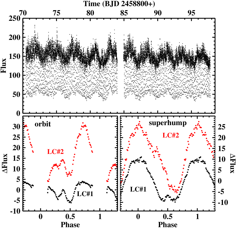
Figure 18: Top: Light curve LC#1 of DW UMa. Bottom: Orbital (left) and superhump waveforms (right) derived from light curves LC#1 (black) and LC#2 (red, shifted vertically for clarity).

3.20 HS 1813+6122: Transient superhumps, transient outbursts, and partial eclipses

Almost all our limited knowledge about the configuration and physics of HS 1813+6122 (HS 1813 hereafter) comes from a single publication: Rodríguez-Gil et al. (2007). They performed photometric and spectroscopic observations on various occasions between 2000 and 2004 and derived an orbital period of 3.55 h. Their photometry also contained a modulation at 3.39 h which they interpreted as a nSH. In contrast to what is seen in the present TESS data (see below) Rodríguez-Gil et al. (2007) apparently did not observe outburst of HS 1813, nor could they identify eclipses. Based on the spectroscopic evidence they classify the system as a SW Sex type star.

TESS observed HS 1813 in many sectors, permitting to construct two almost half year long light curves (LC#1 and LC#2), separated by just one month, and two shorter light curves at later epochs (see Table 1). The flux level differs strongly and systematically from one sector to the next. This cannot be real and must be attributed to difficulties to define the zero point of flux for the TESS light curves. The discontinuous flux levels thus required to add or subtract constants when stitching together data from different sectors to form a continuous light curve. This introduces considerable uncertainties in the general trend of the resulting curves, but should not affect relative variations within a given sector or high frequency variations.

The upper and lower right hand frames of Fig. 19 show LC#1 and LC#2, respectively, binned in intervals of 0.5 d. They contain quite unusual and surprising features. The single sector light curve LC#3 only contains low level variations, while the longer LC#4 is not unlike LC#1. Disregarding the long term trends which may well be artificial (see above), the light curve is characterized by some brightenings above an otherwise quiescent background (LC#1), and then rapidly morphs into a decidedly dwarf nova like light curve (LC#2). Due to the uncertainty of the flux zero point it is difficult to determine the amplitude of the outbursts. Assuming that the flux scale of LC#2 is at least approximately correct, the amplitude reached up to $\approx$0.5 mag and thus remained considerably below normal dwarf nova outburst amplitudes. The rapid change in behaviour between LC#1 and LC#2 which is also manifest in other than the outburst characteristics (see below) is rather unique. I am not aware of another CV which has been observed to behave similarly with the possible exception of the transient ER UMa-type behaviour of BK Lyn (Sect. 3.11). This certainly deserves a deeper investigation, but is not the topic of this study.

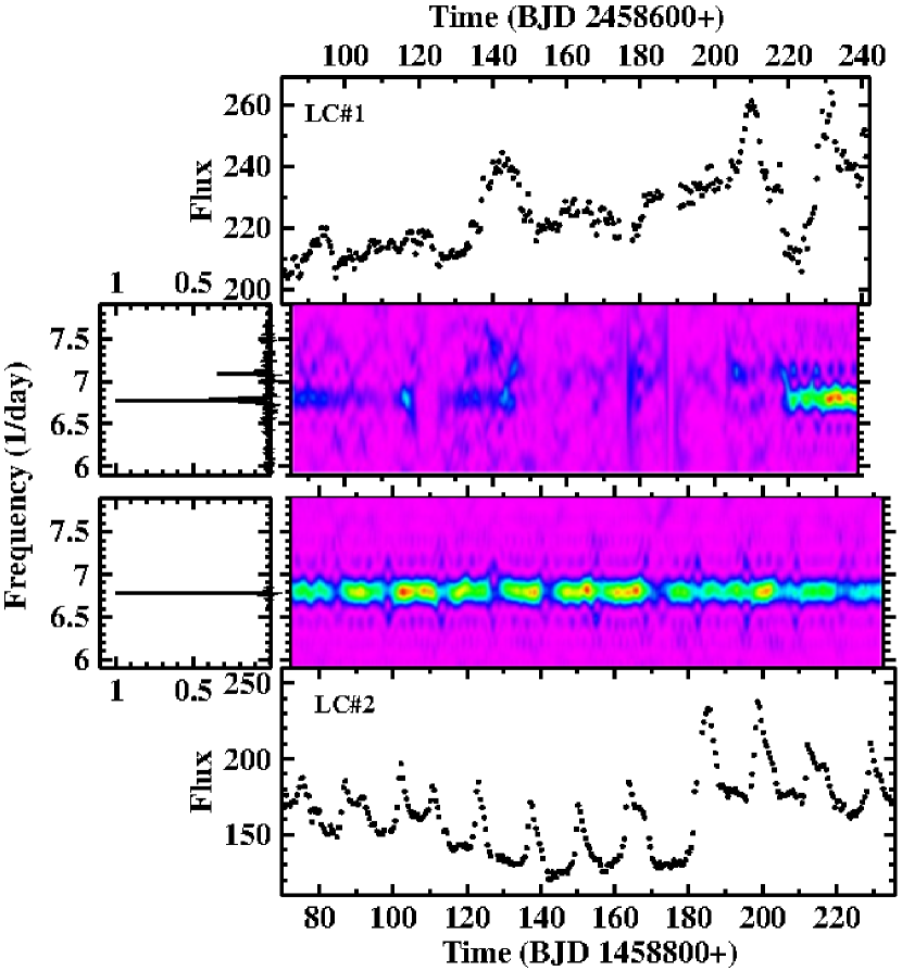
Figure 19: Light curves LC#1 and LC#2 of HS 1813 and their power spectra. The right upper and lower frames show light curves (binned in intervals of 0.5 d) of a very different general aspect, but close in time. The left frames contain the respective power spectra in a small interval around the orbital (dominating signal) and superhump frequencies (only present in LC#1). The remaining frames show the time resolved power spectra of the same frequency range and aligned in time with the light curves.

The power spectra of all light curves are dominated by signals at the orbital frequency and overtones. Their strengths, however, vary considerably over time as is evident in the time resolved power spectra in the two middle right hand frames of Fig. 19 (the frames on the left side contain the conventional power spectra of the entire light curves in the same frequency range). In LC#1 the orbital signal is present during the first weeks, gets fainter thereafter, and then suddenly increases strongly in power at the end of the light curve. Similar fluctuations in strength are also present in LC#3 and LC#4 (not shown). In constrast, in LC#2, i.e., during the episode of dwarf nova-like outbursts, it remains on a constant high level.

The superhump reported by Rodríguez-Gil et al. (2007) is only present in the latter part of LC#1 and at the same frequency of $F_{\rm SH}=7.0890(5)\,{\rm d}^{-1}$ ($P_{\rm SH}=0.141063(9)$ d) observed by them. It cannot be detected in any of the other light curves and must therefore be considered transient.

Folding the TESS light curves on the orbital period derived from the peak frequency in the power spectra reveals the presence of shallow partial eclipses in HS 1813. Average eclipse epochs for the individual TESS sectors are listed in Table 2. They are used to determined the orbital ephemeris:

$$T_{\rm min}=BJD\,2458693.087\,(2)+0.1475202\,(6)\times E$$ (9)

The period error adds up to a phase uncertainty of $\sim$0.15 at the epoch of the spectroscopic observations of Rodríguez-Gil et al. (2007). This makes it unfortunately impossible to obtain a reliable measure of a difference between the spectroscopic phase and the conjunction between the stellar components of HS 1813 as expected in SW Sex stars, and thus to verify this classification.

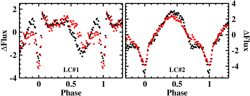
Figure 20: Orbital waveform of HS 1813 during epochs of low (LC1#1, left) and high (LC#2, right) outburst activity. Black symbols refer to outburst epochs, red ones to intervals between outbusts.

The orbital waveforms, as derived from LC#1 and LC#2 are shown in Fig. 20, separately for bright (black) and quiescent (red) intervals. While differences between bright and quiescent intervals remain small, significant changes between LC#1 to LC#2 are evident. In both light curves the waveform is dominated by a broad hump, cut in by a shallow V-shaped (and thus partial) eclipse. In LC#1 the hump is somewhat more structured (possibly doubles) than in LC#2. Moreover, it shifts by 0.3 units to later phases and the minimum broadens in LC#2. This indicates an obvious change in the structure of the dominating light sources in HS 1813. It is close at hand to speculate that this change is somehow related to the onset of the dwarf nova-type brightenings. It is noteworthy, however, that in dwarf novae the waveform normally changes significantly between quiescence and outbursts while this is not the case here.

3.21 RX J2133.7+5107: Superhumps and an unidentified 325 s modulation

This system was detected in the ROSAT Galactic Plane Survey (Motch et al., 1998) and identified by Bonnet-Bidaud et al. (2006) as long period ($P_{\rm orb}=0.297431(5)$ d; Thorstensen et al., 2010) intermediate polar with a white dwarf spin period of 570.82 s. They also saw the orbital side band of the spin period in their power spectra. In a multi-year campaign de Miguel et al. (2017) encountered a nSH with a slightly varying period in all observing seasons between 2010 and 2016.

The TESS light curve confirms these findings. The strongest signal in the power spectrum (left hand frame of Fig. 21) corresponds to a period of 0.28916(3) d which is very close to the average nSH period observed by de Miguel et al. (2017). Just as their observations, the TESS data do not contain a signal at the beat between orbital and superhump period. But in contrast to the former the power spectrum of the latter (weakly) reveals orbital variations. The continued presence of the superhump in all appropriate observations since 2010 allows classifying it as permanent.

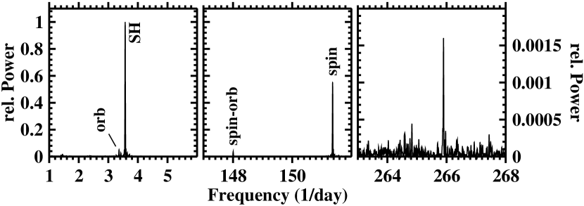
Figure 21: Power spectra of the RX J2133.7+5107 light curve including the superhump and orbital signals (left), the white dwarf spin signal and its orbital sideband (middle) and an unidentified high frequency signal (right). The vertical scale is the same in the left and middle frames, but greatly expanded in the right frame.

Not surprisingly, the power spectrum of the TESS light curves also contains a strong signal at the white dwarf spin period (measured to be 570.8914(5) s; middle panel of Fig. 21), the orbital side band and the first overtone (not shown). de Miguel et al. (2017) also mention signals at $F_{\rm sp}-F_{\rm orb}+F_{\rm SH}$ and $F_{\rm sp}-F_{\rm orb}-F_{\rm SH}$. On close inspection, both of these are also weakly present in the TESS light curve. de Miguel et al. (2017) noted that the spin period is decreasing over the years. The TESS data permit to add an additional point which excellently confirms the linear trend. A least squared fit to all available data yields $d{\rm P}/d{\rm t}=-3.8\pm 0.2$ msec/yr.

While the above results just confirm previous knowledge, the TESS light curves reveals an additional modulation at a high frequency of $F=265.898(2)$ d^-1 ($P=324.937(3)$ s; right hand frame of Fig. 21). It does not have any obvious relation to the other periodicities in the system. Time resolved power spectra reveal that its is persistent – with some variations in its strength – throughout the entire light curve.

The nature of this modulation remains thus unclear. Its coherence over at least two months makes the accretion disk unlikely as the place of origin. I am also not aware of any mechanism inherent in the secondary star which may lead to such short period variations. It may be permitted to speculate about white dwarf pulsations as their origin. The period is within the range observed in well established white dwarf pulsators in CVs such as GW Lib (van Zyl et al., 2004; Chote & Sullivan, 2016, and others) and V455 And (Araujo-Betancor et al., 2005; Szkody et al., 2013; Bruch, 2020). But then, in these stars more than one pulsation mode is excited leading to multiple power spectrum signals, differently from what is observed in RX J2133.7+5107. Moreover, they are short period CVs where the accretion disk is expected to be weak so as not to outshine the white dwarf. At the long period of RX J2133.7+5107 the (precessing) accretion disk and the accretion regions close to the magnetic poles of the WD in this intermediate polar will dominate the optical emission and are thus likely to mask any contribution from the white dwarf itself.

3.22 KIC 8751494: Strongly contaminated TESS light curves

KIC 8751494 was detected as a novalike variable, possibly of the SW Sex subtype, in Kepler data by Williams et al. (2010). They detected variations with a period of 0.1223(7) d. Later Kato & Maehara (2013), also using Kepler data, found this period to be slightly variable and interpreted it as a pSH, the orbital modulations – much fainter than the superhump – having a period of 0.114379(1) d.

The TESS light curves of KIC 8751494 are heavily contaminated by light from the variable star ATO J291.0335+44.9915 (Heinze et al., 2018) which is only 42 arcsec (i.e., twice the TESS pixel size) away. The power spectra (upper left frame of Fig. 22) are strongly dominated by a signal at $F_{\rm ATO}=5.5635(2)$ d^-1 ($P_{\rm ATO}=0.179743(7)$ d) which is compatible with the period listed by Heinze et al. (2018) for ATO-J291.335+44.9915. Signals also appear at multiples of $F_{\rm ATO}$ as well as $F_{\rm ATO}/2$. The latter must be considered as the fundamental frequency. None of them is present in the higher spatial resolution Kepler data. Folding the data on $2P_{\rm ATO}$ (insert in the figure) yields a perfect light curve of a short period Algol system with a secondary eclipse slightly less deep than the primary eclipse. Again, this is compatible with the classification as close eclipsing binary of Heinze et al. (2018). Thus, I attribute these variations exclusively to ATO J291.0335+44.9915. For the record, I give ephemeris for the primary minimum, based on representative minimum epochs measured in the two light curves:

$$T_{\rm min}=BJD\,2458711.16(2)+0.35948(1)\times E$$

Based on only two data points, formal errors are not defined. Therefore, I arbitrarily adopt a period error which would lead to an easily recognizable phase shift of 0.05 of the minimum over the time base of the observations.

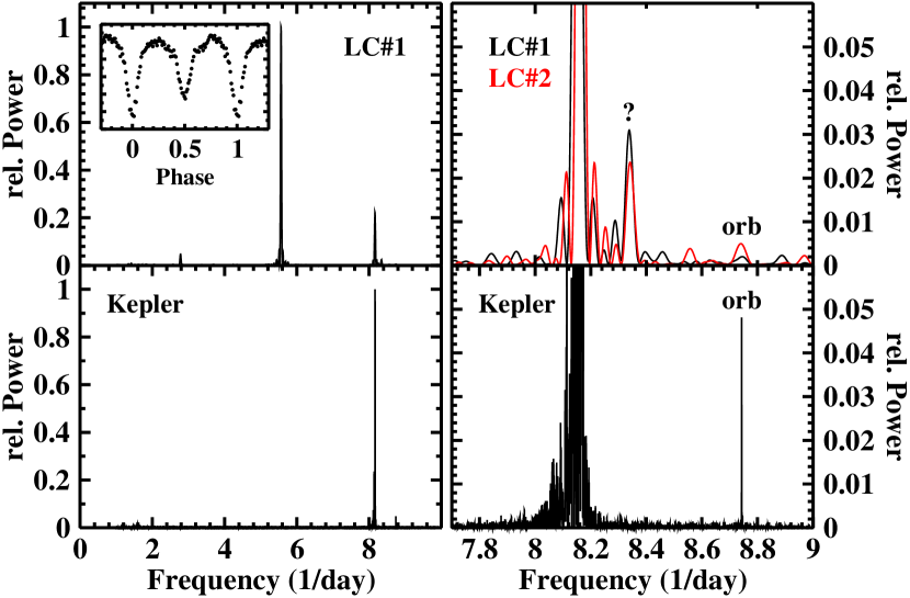
Figure 22: Top left: Power spectrum of LC#1 of KIC 871494. The insert shows the data folded on the period corresponding to half of the frequency of the dominating signal. These variations can be attributed to contamination from the star ATO J291.0335+44.9915 located close to KIC 871494. Top right: Parts of the Power spectra of LC#1 (black) and LC#2 (red) on an expanded scale. Bottom: The same for the power spectrum of the Kepler data of KIC 871494.

In addition to the contamination from ATO J291.0335+44.9915 the TESS power spectra also contain signals coming from KIC 8751494 itself. The SH is clearly present at slightly different frequencies of $F_{\rm SH}=8.152(1)$ d^-1 ($P_{\rm SH}=0.12267(2)$ d) in LC#1 and $F_{\rm SH}=8.1617(3)$ d^-1 ($P_{\rm SH}=0.12252(5)$ d) in LC#2. However, the orbital signal prominently seen in the Kepler data (power spectrum in the lower frames of Fig. 22), is only very weaky present (see right frames of the figure). Instead, the power spectra of the TESS data contain a significant peak between the superhump and the orbital frequencies, marked with a question mark in the figure. The frequency is identical on the $2\sigma$ level in both light curves. The average is $F=8.335(5)$ d^-1 ($P=0.11969(7)$ d). The nature of this additional periodicity is not immediately obvious and I leave this question open.

3.23 KIC 9406652: Alternating positive and negative superhumps

This object was identified as a variable star by Debosscher et al. (2011) in Kepler data. The first detailed investigation, based on low cadence light curves taken during Kepler quarters 1 through 15, was performed by Gies et al. (2013) who pointed out its similarity to old novae and novalike variables. They found the orbital period [later refined by Kimura et al. (2020) to be 0.25451 d], a negative superhump with a period of 0.2397 d, and a supraorbital period of 4.131 d which is the beat between the orbital and SH periods. The light curve is puntuated by semi-regular brightenings which made Kimura et al. (2020) classify KIC 9406652 as an IW And-type star, i.e. an unusual type of Z Cam-type dwarf novae. KIC 9406652 may thus not be a genuine novalike variable. Considering that the TESS data were apparently taken during such a standstill when the accretion disk – just as in the case of AY Psc (Sect. 3.15) – is in a similar hot state as those of NLs and old novae I include KIC 9406652 in this study.

TESS observed the star in 4 sectors. The first and the last two of these, separated in time by about two years (taken in 2019 and 2021, respectively), are consecutive. The data of the latter can be combined into a single light curve. However, those of the former have drastically different flux levels (which may be an artifact considering the known uncertainties concerning the absolute flux scale of TESS light curves) and somewhat distinct properties (see below). Therefore, I prefer not to combine them.

The behaviour of KIC 9406652 is quite different during the two epochs. I first concentrate on the 2019 data [LC#1 and LC#2; Fig. 23: light curves (top), power spectra (middle), and orbital and SH waveforms (bottom)]. Both light curves exhibit variations on time scales of several days. The power spectra reveal signals with periods of several hours. In LC#1, the strongest signal corresponds to a period exactly twice that of the second highest peak and must therefore be interpreted as the first overtone of a modulation with a period of $P=0.2864$(1) d. This period is 12.5% longer than the orbital period $P_{\rm orb}$ which is also manifest in the power spectrum together with its first overtone. It is thus close at hand to identify $P=P_{\rm pSH}$ with the first appearance of a pSH in KIC 9406652. The power spectrum also contains a fainter peak at $F_{\rm pSH}+F_{\rm orb}$ (and still fainter signals at higher overtones of the principal signals), but the beat period $1/F_{\rm pSH}-1/F_{\rm orb}$ and thus the apsidal precession period of the implied eccentric accretion disk is notably absent. The waveform of the orbital modulations (black graph in the bottom frame of Fig. 23) is qualitatively explained by ellipsoidal variations of the secondary star, considering the long period of this system and the red TESS passband, where the secondary minimum is partially filled in by reflection of light from the primary component. In contrast to the easily explained orbital waveform, the shape of the superhump waveform (red graph) is quite peculiar with two peaks of different extension and decidedly pointed minima and maxima.

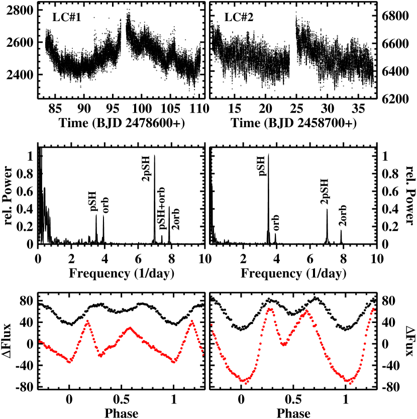
Figure 23: Properties of light curves LC#1 (left column) and LC#2 (right column) of KIC 9406652: light curves (top), low frequency part of the power spectra (middle), and orbital (black) and superhump (red) waveforms (bottom).

In LC#2 the strength of the fundamental superhump mode and its first overtone is inverted. The superhump amplitude is enhanced, and the waveform – still double humped but now superposed upon a single larger maximum – has a much more gentle (rounded) shape. The orbital waveform has not changed much with respect to LC#1. At $P_{\rm pSH}=0.28502(5)$ d the superhump period is slightly but significantly shorter than in LC#1.

In 2021 the light curve of KIC 9406652 was quite different (upper left frame of Fig. 24). It exhibits a clear periodicity on the time scale of several days. The corresponding peak in the power spectrum (lower left frame of the figure) indicates a period of 3.998(9) d which is close to the beat between the orbital period and the period $P_{\rm nSH}=0.239197$ (8) d corresponding to the main signal in the power spectrum. The latter is within the range of nSH periods seen in the Kepler data (Kimura et al., 2020). Thus, the negative superhump is back and the positive one has gone. On the scale of the figure the orbital period is only manifest in the power spectrum by its first overtone. This is easily explained by the orbital waveform (upper right frame of the figure) which is somewhat different than in LC#1 and LC#2, having maxima of different height and a deeper secondary minimum. The superhump waveform (lower right) is dominated by a strong maximum with two small humps on top.

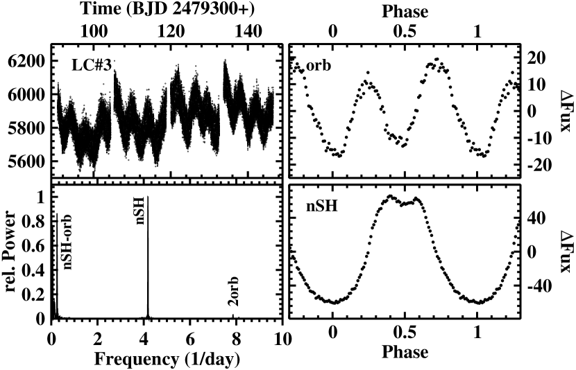
Figure 24: Properties of light curve LC#3 of KIC 9406652: light curve (upper left), low frequency part of the power spectrum (lower left), orbital waveform (upper right) and superhump light curve (lower right).

3.24 NSV 1907: Superhumps confirmed

Discovered as a variable star a long time ago (Hoffmeister, 1963), NSV 1907 (= CRTS J051654.1+33252) remained largely unstudied until quite recently, when Hümmerich et al. (2017) identified it as a deeply eclipsing novalike cataclysmic variable, possibly of the RW Sex subclass. The eclipses permitted them to measured an accurate orbital period of 0.2761069(2) d, i.e., on the longer side of the CV period distribution. A secondary minimum at eclipse phase 0.5 in their white light, $V$ and $B$ light curves attests to a non-negligible contribution of the secondary star at this long period. Hümmerich et al. (2017) also observed a 4.2 d modulation which they interpret as the nodal precession period of an accretion disk and which they use to predict a period of 0.2591 d for a (negative) superhump.

The TESS light observations confirm the presence of the SH as well as the nodal precession period. The light curve is shown in the upper frame of Fig. 25. Apart from the eclipses it is characterized by a strong increase and subsequent decrease of the brightness of NSV 1907 in its second half. Nevertheless the flux at eclipse minimum remains almost the same, meaning that the light source responsible for these variations is largely eclipsed. The out-of-eclipse flux level exhibits wiggles on the time scale of a few days which grow much stronger during the phase of increased brightness in the latter part of the light curve. A power spectrum of the data after removal of the eclipses and the longer term variations contains a strong peak at a frequency of 0.232(2) d^-1. The corresponding period of 4.30(5) d is very close to the period seen by Hümmerich et al. (2017) and thus confirms their results.

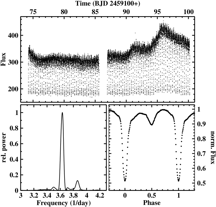
Figure 25: Top: Light curve of NSV 1907. Bottom left: Power spectrum of the light curve in a small range around the orbital frequency. Bottom right: Average waveform of the orbital variations of NSV 1907 normalized such that the eclipse minimum has 50% of the average flux of the two maxima.

At higher frequencies the power spectrum is dominated by signals at the orbital frequency and its overtones even after removal of the eclipses from the light curves. The lower left frame of Fig. 25 shows a narrow range around $F_{\rm orb}$. Apart from the orbital signal is contains a weaker peak at $F_{\rm SH}=3.860(3)$ d^-1 ($P_{\rm SH}=0.2591(1)$ d), leaving no doubt that this is the superhump signal prediced by Hümmerich et al. (2017) but not seen directly in their data.

Finally, the orbital waveform, normalized in the same way as was done for AC Cnc in Paper I, is shown in the lower right frame of Fig. 25. It impressively confirms the presence of secondary eclipses which, not surprisingly, are better defined in the redder TESS passband than in the earlier observations. Before the secondary eclipse the hump in the waveform has a significantly smaller amplitude that afterwards and also appears to have some peculiar structure. I tested if the hump maxima are modulated on the beat period between orbital and SH variations as has been seen in AC Cnc (Paper I). This is indeed the case, but the effect is much smaller than in AC Cnc.

4 Discussion: A census of superhumps

An assessment of superhumps and their implications for the understanding of the structure, dynamics and evolution of CVs has been made many times in the past (e.g., Patterson 1998, 2001, Patterson et al., 2005). A huge body of observational information on pSHs in SU UMa type dwarf nova has been collected by Kato et al. (2009) and in subsequent publications of this series. Much of this work deals with dwarf novae and with pSHs, while specific studies of nSHs and SH in non-outbursting CVs are considerably rarer. Among observational papers with some emphasis on SHs in NLs and old novae I cite Fuentes-Morales et al. (2018). For theoretical studies of nSHs I refer to Thomas & Wood (2015) and citations therein. Concerning our theoretical understanding of pSHs, I mention the classical papers of Whitehurst (1988), Whitehurst & King (1991) and Hirose et al. (1991).

Table 4 contains a census of the properties of positive and negative superhumps in all novae and novalike variables for which I could find reports on such variations in the literature. Apart from the orbital period it lists the SH period (which is many cases is the average of several slightly different values measured at different epochs) and the period excess defined as $\epsilon=\left(P_{\rm SH}-P_{\rm orb}\right)/P_{\rm orb}$. The table also provides information about the SH waveform, the detection or not of the apsidal or nodal precession period in the light curves, and the frequency of occurrence of SHs. I define three categories for the waveform: S indicates an approximately sinusoidal waveform which includes slight deviations from a pure sine such as a sawtooth shape, DH stands for a double humped waveform, and C is used for more complex shapes. Of course, these distinctions (in particular between DH and C) are sometimes subjective. The presence or absence of variations on the disk precession period is indicated by Y(es) or N(o) only in those cases where information in the literature permits a secure statement. The occurrence of superhumps is categorized as permanent (P) whenever it is seen in all available observations (but see below), and as transient (T) when it is seen in some observations but not in others.

Table 4: Summary of positive and negative superhump properties observed in novalike variables and old novae. All periods are expressed in days.

Name	$P_{\rm orb}$	negative superhump					positive superhump					Ref.a
		$P_{\rm nSH}$	$\epsilon_{\rm nSH}^{b}$	WFc	Precd	Occe	$P_{\rm pSH}$	$\epsilon_{\rm pSH}^{b}$	WFc	Precd	Occe
CP Pup	0.06139						0.06250	0.0181	S	N	T	3
BK Lyn	0.07494	0.07280	-0.0286	S	N	T	0.07848	0.0472	S/C	Y	P	1,4,5,6
V1974 Cyg	0.08126						0.08507	0.0469	S	Y	P	1,7,8,9
V348 Pup	0.10184						0.10740	0.0546	S/C	Y	T	1,10
V795 Her	0.10825	0.10474	-0.0324	C	N	T	0.11619	0.0733	S	N	T	2,11-18
KIC 8751494	0.11438						0.12249	0.0709	S	N	P	1,19,20
V592 Cas	0.11506	0.11193	-0.0272	S	N	T	0.12239	0.0637	S/DH	N	P	1,21
DM Gem	0.11570						0.12423	0.0737	S	N	P?	2,22
V630 Sgr	0.11793						0.12417	0.0529	?	Y	T	23,24
LQ Peg	0.11850						0.12480	0.0532	?	Y	P	25,26
V1084 Her	0.12056	0.11696	-0.0299	S	Y	?						27
V442 Oph	0.12443	0.12090	-0.0284	S	Y	P?						27
V4633 Sgr	0.12557						0.12823	0.0212	S	N	T	24,28
AH Men	0.12721	0.12355	-0.0288	S	Y	T	0.13886	0.0916	S	N	T	1,29-31
MV Lyr	0.13290	0.12816	-0.0357	S	N	T	0.13790	0.0376	S	Y	T	2,32,33
DW UMa	0.13661	0.13264	-0.0291	S	Y	T	0.14478	0.0598	S	Y	P	1,34
TT Ari	0.13755	0.13296	-0.0334	S	Y	P	0.14927	0.0852	S	N	T	2,35-50
V603 Aql	0.13822	0.13390	-0.0313	S	N	T	0.14548	0.0525	S	Y	P	51-58
V378 Peg	0.13858	0.13476	-0.0276	S		P						59,60
RR Cha	0.14010	0.13621	-0.0278	S		P	0.14442	0.0308		N	T	1,61
AQ Men	0.14147	0.13646	-0.0354	S	Y	P	0.15047	0.0636	C	Y	T	2,62,63
LS Cam	0.14238	0.13753	-0.0341		Y	P	0.15485	0.0876		N	T	64
V751 Cyg	0.14458	0.13936	-0.0361	S	Y	P						1,65,66
RR Pic	0.14503						0.15770	0.0874	S	N	T	1,67,68
IM Eri	0.14563	0.13841	-0.0496	S	Y	P						62
PX And	0.14634	0.14150	-0.0331	S	Y	T						1,69
V533 Her	0.14737	0.14289	-0.0304		N	T	0.15706	0.0658	S	Y	T	2,70
HS 1813+6122	0.14752	0.14095	-0.0445	S	N	T						1,71
V2574 Oph	0.14773	0.14164	-0.0412	S		T						72
BB Dor	0.14923	0.14093	-0.0556	S	Y	P	0.16330	0.0943	S		T	1,73
AO Psc	0.14950						0.16580	0.1090			T	1,74
BZ Cam	0.15369						0.15634	0.0172	DH		T	1,75
V704 And	0.15424	0.14772	-0.0423	S	Y	T						2
BH Lyn	0.15588	0.14700	-0.0570			T	0.16772	0.0760	S	Y	T	2,76,77
BG Tri	0.15844	0.15150	-0.0438	S	Y	T	0.17270	0.09000	S		T	78
KR Aur	0.16274	0.15713	-0.0345	S		T						1,79
V1193 Ori	0.16500	0.15883	-0.0374	S	N	T	0.17622	0.0680	DH/C	N	T	2
UU Aqr	0.16580						0.17510	0.0561			T	1,73
UX UMa	0.19667	0.18668	-0.0508	S		T						1,26,80
AY Psc	0.21732	0.20640	-0.0502	S		T						1,81
TV Col	0.22860	0.21611	-0.0546	S	Y	T						2,82-85
RW Tri	0.23188	0.22190	-0.0430	S		T						2,26,86
KIC 9406652	0.25451	0.22945	-0.0985	S	Y	T	0.29071	0.1422	C	N	T	1,87,88
NSV 1907	0.27611	0.25910	-0.0616	S	Y	P?						1,89
RX 2133.7+5107	0.29743	0.28132	-0.0542	S	N	P						1,90
RZ Gru	0.41750						0.52000	0.2455	S			2
a References (see Table 5)
b Period excess defined as $\epsilon=\left(P_{\rm SH}-P_{\rm orb}\right)/P_{\rm orb}$
c Waveform: S = sinusoidal; DH = double humped; C = complex
d Precession period detected (Yes/No)
e Occurrence of superhump: P = permanent; T = transient

Table 5: References to Table 4

(1) This work; (2) Paper I; (3) Patterson & Warner (1998); (4) Skillman & Patterson (1993) (5) Misselt & Shafter (1995);

(6) Patterson et al. (2013); (7) Semeniuk et al. (1994); (8) Semeniuk et al. (1995); (9) Retter et al. (1997); (10) Rolfe et al. (2000);

(11) Mironov et al. (1983); (12) Baidak et al. (1985); (13) Kałuzny (1989); (14) Rosen et al. (1989); (15) Shafter et al. (1990);

(16) Zhang et al. (1991); (17) Papadaki et al (2006); (18) Šimon et al. (2012); (19) Williams et al. (2010);

(20) Kato & Maehara (2013); (21) Taylor et al. (1998); (22) Rodríguez-Gil & Torres (2005); (23) Woudt & Warner (2001);

(24) Mróz et al. (2015); (25) Rude & Ringwald (2012); (26) Bruch (2020); (27) Patterson et al. (2002);

(28) Lipkin & Leibowitz (2008); (29) Buckley et al. (1993) (30) Patterson (1995); (31) Patterson (1998); (32) Borisov (1992);

(33) Skillman et al. (1995); (34) Boyd et al. (2017); (35) Andronov et al. (1992); (36) Andronov et al. (1999);

(37) Belova et al. (2013); (38) Bruch (2019b); (39) Kim et al. (2009); (40) Kraichva et al. (1999); (41) Rössiger (1988);

(42) Semeniuk (1987); (43) Skillman et al. (1998); (44) Smak & Stȩpień (1975); (45) Sztanjo (1979); (46) Tremko et al. (1992);

(47) Udalski (1988); (48) Volpi et al. (1998); (49) Weingrill et al. (2009); (50) Wu et al. (2002); (51) Bruch (1991);

(52) Bruch & Cook (2018); (53) Haefner (1981); (54) Haefner & Metz (1985); (55) Hollander et al. (1997);

(56) Patterson et al. (1997); (57) Patterson & Richman (1991); (58) Patterson et al. (1993); (59) Kozhevnikov (2012);

(60) Ringwald et al. (2012); (61) Woudt & Warner (2002); (62) Armstrong et al. (2013); (63) Iłkiewicz et al. (2021);

(64) Rawat et al. (2022); (65) Patterson et al. (2001); (66) Papadaki et al. (2009); (67) Fuentes-Morales et al. (2018);

(68) Schmidtobreick et al. (2008); (69) Stanishev et al. (2002); (70) McQuillin et al. (2012); (71) Rodríguez-Gil et al. (2007);

(72) Kang et al. (2006); (73) Patterson et al. (2005); (74) Patterson (2001) (75) Kato & Uemura (2001); (76) Stanishev et al. (2006);

(77) Patterson (1999); (78) Stefanov et al. (2022); (79) Kozhevnikov (2007); (80) de Miguel et al. (2016);

(81) Gülsecen et al. (2009); (82) Augusteijn et al. (1994); (83) Barrett et al. (1988); (84) Hutchings et al. (1981); (85) Motch (1981);

(86) Smak (2019); (87) Gies et al. (2013); (88) Kimura et al. (2020); (89) Hümmerich et al. (2017); (90) de Miguel et al. (2017).

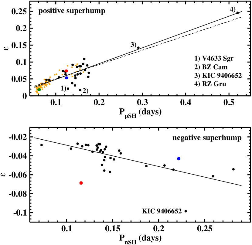
Figure 26: Top: Relation between the period excess and the superhump period for positive superhumps. The large dots represent data taken from Table 4. For comparison, data taken from table 9 of Patterson et al. (2005) are also plotted as smaller orange dots. The solid line is a linear least squares fit to all data from Table 4, excluding the low credential superhump systems V4633 Sgr and BZ Cam. The dashed line is the same, additionally excluding the long period systems KIC 9406652 and RZ Gru. The red, blue and green dots represent DM Gem, LQ Peg, and CP Pup, respectively. For further details, see text. Bottom: The same for negative superhumps. The red and blue dots represent DM Gem under the assumption that it is a negative superhumper, and the low credential system RW Tri, respectively. The solid line is a linear least squares fit to all points except DM Gem.

Some of the stars listed in the table may have low credentials as superhumpers because of sparse of observations, weak indications for SHs, or alternative explications for the observed variations. They are included in the table anyway for the sake of completeness, but it should be kept in mind that they may not exhibit genuine superhumps. In particular, I mention: (1) CP Pup. Patterson & Warner (1998) observed an unstable period which they interpreted as being due to a SH. As I showed in Paper I the TESS light curves of CP Pup exhibit a multitude of transient QPO-like variations in the respective period range which cannot be considered to be superhumps and which in more limited terrestrial observations may mimick SHs. (2) BZ Cam. This case is similar to CP Pup. Kato & Uemura (2001) claim to have seen superhumps, but the multitude of power spectrum peaks in the data of Patterson et al. (1996) and the time resolved power spectrum in Fig. 3 suggest only the occurrence of QPO-like variations. (3) RZ Gru. This star was identified in Paper I as a system with pSHs, but the corresponding power spectrum peak may not be outstanding enough to provide convincing evidence. Moreover, at the long orbital period RZ Gru is not expected to develop a precessing accretion disk (however, I try to avoid a bias based on theoretical preconceptions). (4) RW Tri. This system is claimed to have exhibited nSHs restricted to the 1984 and possibly 1957 observing seasons (Smak, 2019), but not in other years (Bruch, 2020). While this alone does not discredit it as a transient SH system, I consider the peaks in Smak’s power spectra, on which he bases his claim, not of suffient strength to convincingly indicate a consistent periodicity. (5) V4633 Sgr. Fuentes-Morales et al. (2018) list this star as a superhumping old nova, but Lipkin & Leibowitz (2008) interpret the corresponding variations in an asynchronous polar scenario, where the rotation of a magnetic white dwarf got out of synchronization with the orbital period as a consequence of the recent nova outburst of V4633 Sgr in 1998. (6) LQ Peg. It is not clear if the consistent photometric variations in this star are due to the orbital motion or a superhump. For a thorough discussion of this issue, see Bruch (2020). (7) AO Psc. As noticed in Sect. 3.14, AO Psc is only briefly mentioned as a superhumper by Patterson (2001), while the announced publication of details never occurred.

Including the systems with low credentials, Table 4 contains 46 stars. Of these, 30 exhibit positive and 33 negative superhumps. Thus, statistically among novae and novalike variable both species are about equally probable, unless there is an observational bias favouring the detection of one over the other. In nine stars both kinds of SHs have even been seen simultaneously (V603 Aql, TT Ari, LS Cam, V592 Cas, RR Cha, BB Dor, BK Lyn, AQ Men, DW UMa).

Stolz & Schoembs (1984) were the first to note a linear relationship between the period excess $\epsilon$ and the superhump period $P_{\rm SH}$ in SU UMa type dwarf novae; a relationship which – albeit less strictly – is also valid for pSHs in other CVs. It has been refined and discussed many times in subsequent years and sometimes replaced by a relation between $P_{\rm orb}$ and $P_{\rm SH}$ (e.g., Gänsicke et al., 2009; Fuentes-Morales et al., 2018). Both relations are largely equivalent, but if $\epsilon$ vs $P_{\rm SH}$ is linear, $P_{\rm orb}$ vs $P_{\rm SH}$ becomes notably nonlinear if a wider range of periods is regarded. Therefore, I use here the original notation of the Stolz-Schoembs relation.

For all positive superhump systems listed in Table 4, $\epsilon$ is plotted as a function of $P_{\rm pSH}$ as large dots in the upper frame of Fig. 26. For comparison, the respective data taken from table 9 of Patterson et al. (2005) are drawn as smaller orange dots. The bulk of them refers to short period SU UMa type dwarf novae. Several lessons can be learned from this diagram. As is already obvious from the data of Patterson et al. (2005) and is also mentioned by Fuentes-Morales et al. (2018), the scatter of the points corresponding to nova and novalike variables (i.e., almost all points with $P_{\rm pSH}>0.1$ d) exhibit a much higher scatter than the dwarf novae below the CV period gap. Thus, the Stolz-Schoembs relation becomes less well defined for these systems. There are some outliers with low $\epsilon$ values, two of which (V4633 Sgr and BZ Cam) can be identified with low credential superhump systems. These two are ignored subsequently. In contrast, other systems with low credentials – CP Pup (green dot in the figure) and LQ Peg (blue dot) – follow the general trend well. For LQ Peg this may be an indication that the persistent light curve variability is indeed due to SHs and not the orbital motion. DM Gem (red dot) was found in Paper I to exhibit two periods. But it could not be decided which of these is due to the orbital motion and which to SHs. In Fig. 26 DM Gem follows the general trend; a good argument in favour of its interpretation of a positive (instead of negative) superhumper.

Two systems, not previously discussed in the context of the Stolz-Schoembs relation, extend this relation to much longer periods: KIC 9406652 and RZ Gru. While the credentials for superhumps in RZ Gru may not be totally convincing (see above) there is no doubt about the strong pSH in KIC 9406652 (see Sect. 3.23). Excluding these two stars, a linear least squares fit the to remaining points yields the dashed line in Fig. 26. In spite of their significantly longer periods the points corresponding to KIC 9406652 and RZ Gru lie only $0.8\sigma$ and $1.3\sigma$, respectively above the extrapolated $P_{\rm pSH}-\epsilon$ relation defined by the other systems, where $\sigma$ is the standard deviation of their scatter around the dashed line. Thus, both of the long period systems follow well the Stolz-Schoembs relation for nova and novalike stars. The solid line is a least squares fit to all data, yielding $\epsilon=0.002(3)+0.47(2)\,P_{\rm psh}$.

KIC 9406652 and RZ Gru present a challenge to theoretical explanations of pSHs. As mentioned in the Introduction, these are thought to be caused by the extra tidal stresses in the outer regions of an asymmetric accretion disk when its elongated part extends towards the secondary star. The disk can become elliptical when the revolution period of particles in its outer part reaches the 3:1 resonance with the orbital period (Whitehurst, 1988). This is expected to be possible only in systems with a small mass ratio $q=M_{\rm WD}/M_{\rm sec}$. Just how small $q$ must be is a matter of debate. Limits cited in the literature range from 0.22 to 0.39 (Whitehurst & King, 1991; Pearson, 2006; Smak, 2020). The mass ratio of RZ Gru is unknown. Assuming the secondary star to have a mass according to the semi-empirical mass-period relation of Knigge et al. (2011) and the white dwarf mass to be equal to the average mass of the compact object in CVs (Zorotovic et al., 2011) the mass ratio is 0.41, higher than but still close to the upper limit of the theoretically permitted range. Based on radial velocity measurements of absorption and emission lines Gies et al. (2013) derived $q=0.83\pm 0.07$ for KIC 9406652, way beyond this range.

As also outlined in the Introduction, the phenomenological understanding of nSHs as arising in a warped or tilted accretion disk is widely accepted. But their is no consensus on the mechanisms which cause the warp or inclination of the disk. In contrast to positive superhumps it is therefore not possible to specify any limits imposed by theory on the occurrence of negative superhumps and to confront such limits with observations. The $\epsilon-P_{\rm nSH}$ relation constructed from Table 4 is shown in the lower frame of Fig. 26. I also insert as a red dot the location of DM Gem under the assumption that it is a negative superhumper. It falls drastically below the general trend. This is thus a further argument in favor to a pSH nature of this system. The low credential system RW Tri (blue dot) follows the general trend reasonably well and may thus in fact exhibit superhumps sporadically. This leaves KIC 9406652 as the only true outlyer in the diagram with a much more negative period excess than expected at its period. There is, however, no reason to suspect anything to be wrong with its SH period. A linear least squares fit to the data points (including KIC 9406652 but, of course, not DM Gem) yields $\epsilon=-0.006(2)-0.22(1)\,P_{\rm nSH}$ and is shown as a solid line in the figure. I note that the ratio of the inclination of this relation to the corresponding relation for pSHs is $-0.48$, confirming the conventional wisdom that the period deficit in negative superhumps systems is about half of that of the period excess in their positive counterparts at a given period.

In most cases where the corresponding information is available the negative as well as the positive SHs have a roughly sinusoidal shape, consisting of a single hump extending over all phases. Sometimes, it is distorted into a saw tooth with the steeper side leading or trailing, or the maximum is broader or narrower than the minimum. Often the waveform changes somewhat from one epoch to another. More interesting are the rarer cases of double humped or complex waveforms which occur more frequently in positive than in negative superhump systems. Extreme examples are observed in AQ Men (Iłkiewicz et al., 2021), V348 Pup (Fig. 14) or KIC 9406652 (Fig. 23). Such waveforms constitute a valuable source of information about the mechanisms leading to superhumps and the struture of superhumping accretion disks which has not yet been tapped adequately.

Often superhumps are accompanied with variations on the beat period between orbital and SH periods, i.e., at the precession period of the accretion disk. Particularly impressive examples are V348 Pup (Fig. 14) and DW UMa (Fig. 18). But in about a third of all cases variations on the beat period have not been detected. Sometimes this may be explained by absent or only weak variations on the orbital period, but there are counterexamples. The orbital and SH signals are of comparable strength in the power spectrum of the first half of the TESS light curve of V795 Her (Paper I), yet no signal is seen at the beat frequency. In contrast, the orbital is much weaker than the superhump signal in BK Lyn, but the light curve prominently exhibits variations on the beat period (Fig. 11). Of especial interest are a few systems where supraorbital periods are not seen on the beat period but on multiples thereof. These are V603 Aql (Bruch & Cook, 2018), RZ Gru (Paper I) and possibly V1974 Cyg (Sect. 3.8).

With a limited number of observations it is, of course, never possible to be certain that superhumps in any CV are really permanent. Here, I classify a system tentatively as a permanent superhumper if observations at different epochs are available and superhumps were always found when they have been searched for in data of suitable quality and quantity, and unless they are substituted by other long-term features in the light curve [such as the temporary substitution of negative by positive superhumps or the temporary transition into a low state in TT Ari; Bruch (2020)]. In this sense, the most convincing permanent SH systems are V603 Aql (pSH) and TT Ari (nSH; see the numerous references cited in Table 4). Classifying a system as a transient superhumper is much more straightforward: it is sufficient if superhumps are seen at one or several epochs but not at others. Adopting this criterium, transient superhumps are significantly more frequent than permanent ones.

5 Summary

In this paper, I took advantage of the enormous richness of information of the month long (or many times even longer) almost continuous high cadence light curves provided by the TESS mission to explore the properties and the temporal behaviour (periods, occurrence or absence, waveforms, interplay with orbital periods) of superhumps, either negative of positive, in the majority of novalike variables and old novae where such phenomena were observed in the past and for which TESS data are available. The results of this study, in combination with Paper I and information collected from the literature enabled a more complete census of the superhump properties in these systems than was possible hitherto. This compilation of old and new observational attributes should serve to provide boundary conditions for physical models for superhumps. In this context I draw special attention to the sometimes vexing morphological complexity and temporal variability of SH waveforms which merit more attention than they received so far.

As a corollary, for the eclipsing CVs among the targets of this study, eclipse epochs were derived from the TESS data. In some cases these were used together with additional eclipse epochs measured in archival terrestrial light curves to update the sometimes decades old orbital ephemeries and to discuss systematic or erratic period variations.

It is common knowledge that pSHs are abundant – even a defining characteristic – in superoutbursts of short period dwarf novae (SU UMa stars). SHs – both, positive and negative ones – are not observed as routinely in the longer period NLs and old novae, but the fraction of such systems exhibiting SHs is by no means small. The identification of several more such systems in Paper I suggests that many more superhumpers lurk amoung those systems which have not yet been systematically investigated for SHs. TESS light curves of a significant number of such NLs and old novae are available. An effort to analyse these is currently underway and will hopefully lead to a third paper of this small series.

Data availability

All data used in the present study are publically available at the Barbara A. Mikulski Archive for Space Telescopes (MAST:
https://mast.stsci.edu/portal/Mashub/clients/MAST/
Portal.html), the AAVSO web site (https://www.aavso.org) and the LNA Data Bank (http://databank.lna.br).

Appendix A Additional eclipse timings

Table 6: UU Aqr eclipse epochs (zero point for cycle counts as defined by Eq. 1).

Epoch (BJD)	Cycle	Epoch (BJD)	Cycle	Epoch (BJD)	Cycle	Epoch (BJD)	Cycle	Epoch (BJD)	Cycle
(2400000+)	No.	(2400000+)	No.	(2400000+)	No.	(2400000+)	No.	(2400000+)	No.
51755.7281	0	55415.8404	22375	56215.4214	27263	57249.7401	33586	58368.6292	40426
51756.5464	5	55416.6578	22380	56507.5749	29049	57262.4991	33664	58369.4481	40431
51756.7100	6	55416.8217	22381	56507.7392	29050	57609.4530	35785	58369.6107	40432
53234.6594	9041	55417.6403	22386	56508.5574	29055	57617.4687	35834	58370.4295	40437
54322.4696	15691	55417.8032	22387	56508.7214	29056	57627.6106	35896	58370.5924	40438
54323.4510	15697	55418.6214	22392	56509.5399	29061	57627.7741	35897	58370.7575	40439
54325.4128	15709	55418.7846	22393	56509.7027	29062	57628.5922	35902	58371.5731	40444
54357.4749	15905	55469.4949	22703	56510.6839	29068	57628.7564	35903	58371.7378	40445
54365.4905	15954	55778.4979	24592	56510.6842	29068	57629.5739	35908	58372.5563	40450
54728.4749	18173	55795.5097	24696	56523.4439	29146	57629.7363	35909	58372.7188	40451
54731.4211	18191	55799.5995	24721	56563.5208	29391	57630.5556	35914	58373.5371	40456
54734.5267	18210	55799.7637	24722	56563.5209	29391	57630.7185	35915	58373.7004	40457
54734.6915	18211	55800.5812	24727	56563.6837	29392	57642.4966	35987	58374.5178	40462
54735.3454	18215	55800.7451	24728	56563.6837	29392	57991.7407	38122	58377.6263	40481
54736.3271	18221	55801.5633	24733	56872.6888	31281	57995.6656	38146	58378.4439	40486
54810.2672	18673	55801.7268	24734	56872.8515	31282	58349.6548	40310	58378.6062	40487
54830.2252	18795	55893.3309	25294	56874.6512	31293	58349.8171	40311	58726.5426	42614
55059.3979	20196	56157.6775	26910	56874.8140	31294	58350.4714	40315	58726.7062	42615
55106.3460	20483	56159.4761	26921	56893.4627	31408	58351.6177	40322	58733.5766	42657
55415.6770	22374	56160.4586	26927	57249.5761	33585	58351.7801	40323

Table 7: V348 Pup eclipse epochs (zero point for cycle counts as defined by Dai et al. (2010)).

Epoch (BJD)	Cycle	Epoch (BJD)	Cycle	Epoch (BJD)	Cycle	Epoch (BJD)	Cycle	Epoch (BJD)	Cycle
(2400000+)	No.	(2400000+)	No.	(2400000+)	No.	(2400000+)	No.	(2400000+)	No.
56631.6506	78948	56633.6873	78968	57008.7600	82651	57728.7619	89721	57729.7803	89731
56633.5858	78967	56633.7889	78969	57728.6603	89720	57729.6783	89730

Table 8: RW Tri eclipse epochs (zero point for cycle counts as defined by Eq. 7).

Epoch (BJD)	Cycle	Epoch (BJD)	Cycle	Epoch (BJD)	Cycle	Epoch (BJD)	Cycle	Epoch (BJD)	Cycle
(2400000+)	No.	(2400000+)	No.	(2400000+)	No.	(2400000+)	No.	(2400000+)	No.
53672.6223	0	56228.4405	11022	57328.2638	15765	57337.5394	15805	57409.6550	16116
54392.3882	3104	56609.4252	12665	57329.4233	15770	57338.6984	15810	57410.5828	16120
54419.5180	3221	56619.3963	12708	57329.6556	15771	57339.3944	15813	57415.6840	16142
54447.3442	3341	56636.3240	12781	57329.8875	15772	57340.3218	15817	57416.6113	16146
54835.2862	5014	56922.4676	14015	57330.5834	15775	57342.4087	15826	57419.3941	16158
55063.4584	5998	56933.3661	14062	57330.8145	15776	57343.3362	15830	57420.3215	16162
55106.3577	6183	56935.4533	14071	57331.2785	15778	57344.2639	15834	57421.4813	16167
55172.4441	6468	57314.3506	15705	57331.5104	15779	57345.4232	15839	57422.4087	16171
55487.3422	7826	57315.7423	15711	57332.6698	15784	57391.7998	16039	57423.3364	16175
55490.3565	7839	57317.5974	15719	57332.9016	15785	57397.8289	16065	57424.4957	16180
55533.4868	8025	57319.6843	15728	57333.3658	15787	57399.6844	16073	57424.7273	16181
55822.4132	9271	57320.3800	15731	57334.2930	15791	57400.3797	16076	57623.4522	17038
55828.4424	9297	57321.3071	15735	57334.5248	15792	57400.6118	16077	57642.4662	17120
55867.3985	9465	57321.5389	15736	57334.7571	15793	57401.7710	16082	57645.4807	17133
55881.3116	9525	57324.5538	15749	57335.4523	15796	57402.6986	16086	57684.9010	17303
55950.4122	9823	57326.4088	15757	57335.9160	15798	57403.3943	16089	57685.5961	17306
55953.4270	9836	57326.6406	15758	57336.3799	15800	57403.6260	16090	57685.8285	17307
55957.3700	9853	57327.3361	15761	57336.6115	15801	57407.5681	16107	57686.7559	17311
56200.3826	10901	57327.5684	15762	57336.8436	15802	57408.7277	16112	58431.3325	20522

Table 9: UX UMa eclipse epochs (zero point for cycle counts as defined by Eq. 8).

Epoch (BJD)	Cycle	Epoch (BJD)	Cycle	Epoch (BJD)	Cycle	Epoch (BJD)	Cycle	Epoch (BJD)	Cycle
(2400000+)	No.	(2400000+)	No.	(2400000+)	No.	(2400000+)	No.	(2400000+)	No.
43311.7185	-40718	56688.7090	27299	57116.6640	29475	57143.8064	29613	57525.7421	31555
43660.8097	-38943	56725.2894	27485	57117.6483	29480	57144.0029	29614	57526.7250	31560
43998.6925	-37225	56725.4859	27486	57118.4352	29484	57144.3959	29616	57529.6749	31575
48779.7710	-12915	56731.3853	27516	57119.4182	29489	57144.7893	29618	57530.6580	31580
51319.7821	0	56733.3520	27526	57119.6150	29490	57145.7726	29623	57785.9373	32878
52363.5161	5307	56733.5494	27527	57119.8115	29491	57145.9689	29624	57804.8179	32974
52551.3369	6262	56734.3363	27531	57120.4025	29494	57146.7558	29628	57809.5381	32998
53466.6455	10916	56734.5324	27532	57121.3857	29499	57147.7394	29633	57811.8981	33010
53473.9221	10953	56738.2695	27551	57121.5827	29500	57148.5256	29637	57883.6832	33375
53476.8723	10968	56738.4663	27552	57121.7789	29501	57150.6887	29648	57888.7966	33401
53477.8555	10973	56739.2526	27556	57122.3686	29504	57150.8855	29649	57890.7632	33411
53481.7887	10993	56739.4495	27557	57122.5651	29505	57152.4585	29657	57907.6769	33497
53495.7527	11064	56741.4160	27567	57122.7608	29506	57152.8521	29659	57939.3410	33658
53760.8655	12412	56741.6130	27568	57122.9581	29507	57153.4429	29662	58154.8926	34754
54154.4047	14413	56742.3995	27572	57123.3518	29509	57153.8352	29664	58173.3798	34848
54187.4456	14581	56742.5968	27573	57123.7447	29511	57154.4258	29667	58173.5762	34849
54512.3469	16233	56743.3830	27577	57124.5319	29515	57154.6222	29668	58175.3468	34858
54912.7701	18269	56749.4800	27608	57124.7287	29516	57157.5729	29683	58175.5431	34859
54933.6164	18375	56751.4463	27618	57125.3192	29519	57158.5561	29688	58179.8698	34881
55279.3648	20133	56752.4297	27623	57125.5155	29520	57160.5220	29698	58181.8367	34891
55279.7582	20135	56754.3964	27633	57126.4985	29525	57162.4906	29708	58192.6534	34946
55298.6385	20231	56754.5929	27634	57126.6951	29526	57163.4728	29713	58212.5173	35047
55309.6520	20287	56756.3637	27643	57127.4820	29530	57164.4564	29718	58246.7381	35221
55616.4587	21847	56757.3465	27648	57127.6771	29531	57165.4392	29723	58527.3874	36648
55617.4423	21852	56757.5433	27649	57128.6623	29536	57166.4216	29728	58527.5843	36649
55621.3754	21872	56763.4428	27679	57128.8586	29537	57166.6203	29729	58554.7254	36787
55993.2806	23763	56785.6671	27792	57129.6454	29541	57168.3892	29738	58554.9221	36788
55993.4773	23764	56789.6006	27812	57129.8413	29542	57168.5861	29739	58559.4450	36811
55994.2636	23768	56789.7974	27813	57130.6284	29546	57169.5706	29744	58559.6411	36812
55994.4605	23769	56792.3540	27826	57131.4158	29550	57169.7664	29745	58620.6092	37122
55995.2469	23773	56794.3202	27836	57131.8085	29552	57170.5534	29749	58627.6898	37158
55995.4438	23774	56802.7776	27879	57132.0061	29553	57170.7493	29750	58898.8991	38537
56012.7505	23862	56807.6943	27904	57132.3987	29555	57171.5348	29754	58915.2223	38620
56346.5016	25559	56811.6282	27924	57132.5952	29556	57173.5031	29764	58915.4194	38621
56351.6146	25585	57078.7074	29282	57132.7923	29557	57177.4367	29784	58922.4999	38657
56353.3848	25594	57081.6568	29297	57132.9895	29558	57190.4161	29850	58923.2869	38661
56353.5812	25595	57081.8539	29298	57133.3822	29560	57191.4004	29855	58923.4825	38662
56372.4621	25691	57083.8209	29308	57133.7748	29562	57192.5799	29861	58941.5776	38754
56376.3951	25711	57092.8677	29354	57133.9721	29563	57193.5634	29866	58941.7736	38755
56378.3616	25721	57098.5713	29383	57134.3648	29565	57194.5476	29871	59283.7852	40494
56381.3120	25736	57099.3580	29387	57134.7581	29567	57198.4803	29891	59293.8150	40545
56381.5088	25737	57099.5551	29388	57135.5457	29571	57199.4629	29896	59310.7292	40631
56382.2954	25741	57099.7514	29389	57135.7420	29572	57202.4135	29911	59317.6125	40666
56383.2791	25746	57100.3415	29392	57135.9383	29573	57207.5266	29937	59317.8093	40667
56383.4753	25747	57100.5382	29393	57136.5285	29576	57208.5098	29942	59332.7564	40743
56385.4419	25757	57102.7016	29404	57136.7258	29577	57209.4956	29947	59352.6205	40844
56386.4253	25762	57103.2916	29407	57138.4943	29586	57222.4738	30013	59364.6172	40905
56388.3921	25772	57103.4888	29408	57139.6757	29592	57223.4576	30018	59605.3423	42129
56391.3420	25787	57104.4708	29413	57140.4630	29596	57224.4399	30023	59605.5396	42130
56391.5389	25788	57107.4216	29428	57140.6594	29597	57226.4081	30033	59622.4531	42216
56393.3089	25797	57107.6197	29429	57140.8548	29598	57227.3907	30038	59639.3667	42302
56395.2752	25807	57108.7979	29435	57141.4453	29601	57227.7848	30040	59639.5644	42303
56454.6696	26109	57108.9958	29436	57141.6419	29602	57467.3300	31258	59675.7512	42487
56686.3487	27287	57109.7807	29440	57141.8388	29603	57467.5267	31259	59703.6790	42629
56686.5451	27288	57110.7647	29445	57142.4293	29606	57470.6735	31275	59703.8751	42630
56687.3310	27292	57111.7481	29450	57142.6257	29607	57471.6567	31280
56687.5284	27293	57111.9446	29451	57142.8231	29608	57494.6675	31397
56688.3147	27297	57113.7153	29460	57143.4127	29611	57520.6280	31529
56688.5115	27298	57114.8952	29466	57143.6087	29612	57520.8249	31530

References

- Africano et al. (1978) Africano J.L., Nather R.E., Patterson J., Robinson E.L., Warner B., 1978, PASP, 90, 568
- Africano & Wilson (1976) Africano J.L., Wilson J., 1976, PASP, 88, 8
- Andronov et al. (1999) Andronov I.L., Arai K., Chinorova L.L., et al., 1999, AJ, 117, 574
- Andronov et al. (1989) Andronov I.L., Kimeridze G.N., Richter G.A., Symkov V.P., 1989, IBVS, 3388
- Andronov et al. (1992) Andronov I.L., Kolosov D.E., Movchan A.I., Rudenko A.N., 1992, Soobshch. Spets. Astrofiz. Obs., 69, 79
- Applegate (1992) Applegate J.H., 1992, ApJ, 385, 621
- Araujo-Betancor et al. (2005) Araujo-Betancor S. Gänsicke B.T., Hagen, H.-J., et al., 2005, A&A, 430, 629
- Armstrong et al. (2013) Armstrong E., Patterson J., Michelsen R., et al., 2013, MNRAS, 435, 707
- Augusteijn et al. (1994) Augusteijn T., Heemskerk M.H.M., Zwarthoed G.A.A., van Paradijs J., 1994, A&AS, 107, 219
- Baidak et al. (1985) Baidak A.V., Lipunova N.A., Shugarov S.Yu., Moshkalev V.G., Volkov, L.M., 1985, IBVS, 2676
- Baptista et al. (1995) Baptista R., Horne K., Hilditch R.W., Mason K.O., Drew J.E., 1995, ApJ, 448, 393
- Baptista et al. (1994) Baptista R., Steiner J.E., Cieslinski D., 1994, ApJ, 433, 332
- Barrett et al. (1988) Barrett P., O’Donoghue D., Warner B., 1988, MNRAS, 233, 759
- Beljawsky (1926) Beljawsky P.R., 1926, Beobachtungs-Zirkular der Astron. Nachr., 6, 38
- Belova et al. (2013) Belova A.L., Suleimanov V.F., Bikmaev I.F., Khamitov I.M., Zhukov G.V., Senio D.S., Belov I.Y., Sakhibullin N.A., 2013, Astron. Lett., 39, 111
- Biryukov & Borisov (1990) Biryukov W., Borisov G.V., 1990, Perem. Szvesdy, 1544, 1
- Boeva et al. (2021) Boeva, S., Latev, G., Zamanov R., 2021, ATel, 14365
- Bonnet-Bidaud et al. (2006) Bonnet-Bidaud J.M., Mouchet M., de Martino D., Matt G., Motch C., 2006, A&A, 445, 1037
- Borisov (1992) Borisov G.V., 1992, A&A, 261, 154
- Boyd et al. (2017) Boyd D.R.S., de Miguel E. Patterson J., et al., 2017, MNRAS, 466, 3417
- Bruch (1991) Bruch A., 1991, Acta Astron., 41,101
- Bruch (2019a) Bruch A., 2019a, IBVS, 6257
- Bruch (2019b) Bruch A., 2019b, MNRAS, 489, 2961
- Bruch (2020) Bruch A., 2020, New Astr., 78, 101369
- Bruch (2021) Bruch A., 2021, MNRAS, 503, 953
- Bruch (2022a) Bruch A., 2022a, MNRAS, 509, 4669
- Bruch (2022b) Bruch A., 2022b, MNRAS, 514, 4718
- Bruch & Cook (2018) Bruch A., Cook L.M., 2018, New Astr., 63, 1
- Buckley et al. (1993) Buckley D.A.H., Remillard R.A., Tuohy I.R., Warner B., Sullivan D.J., 1993, MNRAS, 265, 926
- Chen et al. (2001) Chen A., O’Donogue D., Stobie R.S., Kilkenny D., Warner B., 2001 MNRAS, 325, 89
- Chote & Sullivan (2016) Chote P., Sullivan D.J., 2016, MNRAS, 458, 1393
- Dai et al. (2010) Dai Z.B., Qian S.B., Fernández-Lajus E., Baume G.L., 2010, MNRAS, 409, 1195
- Debosscher et al. (2011) Debosscher J., Blomme J., Aerts C., De Ridder J., 2011, A&A, 529, A89
- Deeming (1975) Deeming T.J., 1975, Ap&SS, 39, 137
- de Miguel et al. (2016) de Miguel E., Patterson J., Cejudo E., et al., 2016, MNRAS, 457, 1447
- de Miguel et al. (2017) de Miguel E., Patterson J., Jones J.L., et al., 2017, MNRAS, 467, 428
- DeYoung & Schmidt (1993) DeYoung J.A., Schmidt R.E., 1993, IAU Circ., 5880
- Diaz & Steiner (1990) Diaz M.P., Steiner J.E., 1990, A&A, 238, 170
- Eastman et al. (2010) Eastman, J., Siverd, R., & Gaudi, B.S., 2010, PASP, 122, 935
- Froning et al. (2003) Froning C.S., Long K.S., Baptista R., 2003, AJ, 126, 964
- Fuentes-Morales et al. (2018) Fuentes-Morales I., Vogt, N., Tappert C., 2018, MNRAS 474, 2493
- Gänsicke et al. (2009) Gänsicke B.T., Dillon M., Southworth J., 2009, MNRAS, 397, 2170
- Garnavich & Szkody (1988) Garnavich P., Szkody P., 1988, PASP, 100, 1522
- Gies et al. (2013) Gies D.R., Guo Z., Howell S.B., 2013, ApJ, 775, 64
- Green et al. (1986) Green R.F., Schmidt M., Liebert J., 1986, ApJS, 61, 305
- Greenstein et al. (1970) Greenstein J.L., Sargent A.I., Haug U., 1970, A&A, 7, 1
- Greiner et al. (2001) Greiner J., Tovmassian G., Orio M., et al., 2001, A&A, 376, 1031
- Gülsecen et al. (2009) Gülsecen H., Retter A., Esenoǧlu H., 2009, New Astr., 14, 330
- Haefner (1981) Haefner R., 1981, IBVS, 2045
- Haefner & Metz (1985) Haefner R., Metz K., 1985, A&A, 145, 311
- Han et al. (2017) Han Z., Qian S., Voloshina I., Zhu L., 2017, Research A&A, 17, 56
- Heinze et al. (2018) Heinze A.N., Tonry J.L., Denneau, L., 2018, AJ, 156, 241
- Hellier & Robinson (1994) Hellier C., Robinson E.L., 1994, ApJ, 431, L107
- Hirose et al. (1991) Hirose M., Osaki Y., Mineshige S., 1991, PASJ, 43, 809
- Hoffmeister (1963) Hoffmeister C., 1963, Astron. Nachr., 287, 169
- Hollander et al. (1997) Hollander A., Kraakman H., van Paradijs, J., 1997, A&AS, 101, 87
- Honeycutt (2001) Honeycutt R.K., 2001, PASP, 113, 473
- Honeycutt & Kafka (2004) Honeycutt R.K., Kafka S., 2004, AJ, 128, 1279
- Honeycutt et al. (1994) Honeycutt R.K., Robertson J.W., Turner G.W., Vesper D.N., 1994, in Shafter A.W., ed., ASP Conf. Ser. 56, Interacting Binary Stars, p. 277
- Howell et al. (1991) Howell S.B., Szkody P., Kreidl T.J., Dobrzycka D., 1991, PASP, 103, 300
- Hümmerich et al. (2017) Hümmrich S., Gröbel R., Hambsch F.-J., et al., 2017 New Astr., 50, 30
- Hutchings et al. (1981) Hutchings J.B., Crampton D., Cowley A.P., Thorstensen J.R., Charles P.A., 1981, ApJ, 249, 680
- Hutchings et al. (1983) Hutchings J.B., Link R., Crampton D., 1983, PASP, 95, 265
- Iłkiewicz et al. (2021) Iłkiewics K., Scaringi S., Court J.M.C., et al., 2021, MNRAS, 503, 4050
- Kafka (2021) Kafka S., 2021, Observations from the AAVSO International Data Base available at https://www.aavso.org
- Kałuzny (1989) Kałuzny J, 1989, Acta Astron., 39, 235
- Kang et al. (2006) Kang T.W., Retter A., Liu A., Richards M., 2006, AJ, 131, 1687
- Kato et al. (2009) Kato T., Imada A, Uemura M., et al., 2009, PASJ, 61, S395
- Kato et al. (2002) Kato T., Ishioka R., Uemura M., 2002, PASJ, 54, 1003
- Kato & Maehara (2013) Kato T., Maehara H., 2013, PASJ, 65, 76
- Kato & Starkey (2002) Kato T., Starkey D.R., 2002, IBVS, 5358
- Kato & Uemura (2001) Kato T., Uemura M., 2001, IBVS, 5077
- Kim et al. (2009) Kim Y., Andronov I.L., Cha S.M., Chinarova L.L., Yoon J.N., 2009, A&A, 496,765
- Kimura et al. (2020) Kimura M., Osaki Y., Kato T., 2020, PASJ, 72, 94
- Knigge et al. (2011) Knigge C., Baraffe I., Patterson J., 2011, ApJS, 194, 28
- Kozhevnikov (2007) Kozhevnikov V.P., 2007, MNRAS, 378, 957
- Kozhevnikov (2012) Kozhevnikov V.P., 2012, New Astron., 17, 38
- Kraichva et al. (1999) Kraicheva Z., Stanishev V., Genkov V., Iliev V., 1999, A&A, 351, 607
- Kukarkin (1977) Kukarkin B.V., 1977, MNRAS, 180, 5p
- Lima et al. (2021) Lima I.J., Rodrigues C.V., Ferreira Lopes, C.E., et al., 2021, AJ, 161, 225
- Lipkin & Leibowitz (2008) Lipkin Y.M, Leibowitz E.M., 2008, MNRAS, 387, 289
- Lomb (1976) Lomb N.R., 1976, Ap&SS, 39, 447
- Mandel (1965) Mandel O.E., 1965, Perem. Szvesdy, 15, 475
- McQuillin et al. (2012) McQuillin R., Evans A, Wilson D., Maxtet P.F.L., Placco D., West R.G., Hounsell R.A., Bode M.F., 2012, MNRAS, 419, 330
- Mercado & Honeycutt (2002) Mercado L., Honeycutt R.K., 2002, Bull. AAS, 34, 1162
- Mironov et al. (1983) Mironov A.V., Moshkalev V.G., Shugarov S.Yu., 1983, IBVS, 2438
- Misselt & Shafter (1995) Misselt K.A., Shafter A.W., 1995, AJ, 109, 1757
- Montgomery (2009) Montgomery M.M., 2009, ApJ, 705, 603
- Motch (1981) Motch C., 1981, A&A, 200, 277
- Motch et al. (1998) Motch C., Guillout P., Haberl F., et al., 1998, A&AS, 132,341
- Motch & Pakull (1981) Motch C., Pakull M.W., 1981, A&A, 101, L9
- Mróz et al. (2015) Mróz P., Udalski A., Poleski R., et al., 2015, ApJS, 219, 26
- Nather & Robinson (1974) Nather R.E., Robinson E.L., 1974, ApJ, 190, 637
- Neustroev et al. (2011) Neustroev V.V., Suleimanov V.F., Borisov N.V., Belyakov K.V., Shearer A., 2011, MNRAS, 410, 963
- Norton et al. (1996) Norton A.J., Beardmore A.P., Taylor P., 1996, MNRAS, 280, 973
- Osaki & Kato (2013) Osaki Y., Kato T., 2013, PASJ, 65, 95
- Osaki & Kato (2014) Osaki Y., Kato T., 2014, PASJ, 66, 15
- Papadaki et al. (2009) Papadaki C., Boffin H.M.J., Stanishev V., Boumis P., Akras S., Sterken C., 2009, J. Astron. Data, 15, 1
- Papadaki et al (2006) Papadaki C., Boffin H.M.J., Sterken C., Stanishev V., Cuypers J., Boumis P., Akras S., Alikakos J., 2006, A&A, 456, 599
- Patterson (1995) Patterson J., 1995, PASP, 107, 657
- Patterson (1998) Patterson J., 1998, PASP, 110, 1132
- Patterson (1999) Patterson J., 1999, in: S. Mineshige & J.C. Wheeler (eds.) Disk instabilities in close binary systems, Tokyo Universal Academic Press, p. 61
- Patterson (2001) Patterson J., 2001, PASP, 113, 736
- Patterson et al. (2002) Patterson J., Fenton W.H., Thorstensen J.R., et al., 2002, PASP, 114, 1364
- Patterson et al. (2005) Patterson J., Kemp J., Harvey D.A., et al., 2005, PASP, 117, 1204
- Patterson et al. (1997) Patterson J., Kemp, J., Saad J., Skillman D.R., Harvey D., Fried R., Thorstensen J.R., Ashley R., 1997, PASP, 109, 468
- Patterson et al. (1996) Patterson J., Patino R., Thorstensen J.R., 1996, AJ, 111, 2422
- Patterson & Price (1981) Patterson J., Price C.M., 1981, ApJ, 243, L83
- Patterson & Richman (1991) Patterson J., Richman H., 1991, PASP, 103, 735
- Patterson et al. (1993) Patterson J., Thomas G., Skillman D.R., Diaz M., 1993, ApJS, 86, 235
- Patterson et al. (2001) Patterson J., Thorstensen J.R., Fried R., 2001, PASP, 113, 72
- Patterson et al. (2013) Patterson J., Uthas H., Kemp J., et al., 2013, MNRAS, 434, 1902
- Patterson & Warner (1998) Patterson J., Warner B., 1998, PASP, 110, 1026
- Pearson (2006) Pearson K.J., 2006, MNRAS, 371, 235
- Quigley & Africano (1978) Quigley R., Africano J., 1978, PASP, 90, 445
- Ramsay et al. (2016) Ramsay G., Hakala P., Wood M.A., 2016, MNRAS, 455, 2772
- Rawat et al. (2022) Rawat N., Pandey J.C., Joshi A., Yadava U., 2022, MNRAS, 512, 6054
- Retter et al. (1997) Retter A., Leibowitz E.M., Ofek E.O., 1997, MNRAS, 286, 745
- Ricker et al. (2014) Ricker G.R., Winn, J.N., Vanderspek R., et al., 2014, J. Astr. Tel. Instr. & Systems, 1, 014003
- Ringwald et al. (1996) Ringwald F.A., Thorstensen J.R., Honeycutt R.K., Robertson J.W., 1997, MNRAS, 278, 125
- Ringwald et al. (2012) Ringwald F.A., Velasco K., Roveto J.J., Meyers M.E., 2012, New Astron., 17,433
- Robinson et al. (1991) Robinson E.L., Shretone M.D., Africano J.L., 1991, AJ, 102, 1176
- Rodríguez-Gil et al. (2007) Rodríguez-Gil P., Gänsicke B.T., Hagen, H.J., et al., 2007, MNRAS, 377, 1747
- Rodríguez-Gil & Potter (2003) Rodríguez-Gil P., Potter S.B., 2003, MNRAS, 342, L1
- Rodríguez-Gil et al. (2012) Rodríguez-Gil P., Schmidtobreick, L., Long, K.S., Gänsicke B.T., Torres M.P.A., Rubio Díez M.M., Santander-Garcíia M., 2012 MNRAS, 422, 2332
- Rodríguez-Gil et al. (2020) Rodríguez-Gil P., Shahbaz T., Torres M.P.A., Gänsicke B.T., Izquierdo P., Toloza O., Álvarez-Hernández A., Steeghs D., 2020, MNRAS, 494, 425
- Rodríguez-Gil & Torres (2005) Rodríguez-Gil P, Torres M.P.A., 2005, A&A, 431, 289
- Rössiger (1988) Rössiger R., 1988, Sternwarte Sonneberg, Mitt. Veraenderliche Sterne, 11, 112
- Rolfe et al. (2000) Rolfe D.J., Haswell C.A., Patterson J., 2000, MNRAS, 317, 759
- Rosen et al. (1989) Rosen S.A., Branduardi-Raymont G., Mason K.O., Murdin P.G., 1989, MNRAS, 237, 1037
- Rosen et al. (1994) Rosen S.R., Clayton K.L., Osborne J.P., McGale P.A., 1994, MNRAS, 269, 913
- Rubenstein et al. (1991) Rubenstein E.P., Patterson J., Africano J.L., 1991, PASP, 103, 1258
- Rude & Ringwald (2012) Rude G.D., Ringwald F.A., 2012, New Astr., 17, 453
- Rutten et al. (1992) Rutten R.G.M., van Paradijs J., Tinbergen J., 1992, A&A, 260, 213
- Saito & Baptista (2016) Saito R., Baptista R., 2016, MNRAS, 457, 198
- Savitzky & Golay (1964) Savitzky A., Golay M.J.E., 1964, Analytical Chemistry, 36, 1627
- Scargle (1982) Scargle J.D., 1982, ApJ, 263, 853