On the strong metric dimension of composed graphs

Abstract

Two vertices $u$ and $v$ of an undirected graph $G$ are strongly resolved by a vertex $w$ if there is a shortest path between $w$ and $u$ containing $v$ or a shortest path between $w$ and $v$ containing $u$. A vertex set $R$ is a strong resolving set for $G$ if for each pair of vertices there is a vertex in $R$ that strongly resolves them. The strong metric dimension of $G$ is the size of a minimum strong resolving set for $G$. We show that a minimum strong resolving set for an undirected graph $G$ can be computed efficiently if and only if a minimum strong resolving set for each biconnected component of $G$ can be computed efficiently.

0.1 Introduction

In this paper we consider the strong metric dimension introduced by Sebö and Tannier in [ST04]. The strong metric dimension is a variant of the original metric dimension (which we simply call metric dimension) which is the smallest number $k$ of vertices from which the vector of distances to every vertex in the graph is unique. Here the distance between two vertices is the number of edges on a shortest path. The $k$-dimensional distance vectors of the vertices can be viewed as their positions in a $k$-dimensional space whose structure is defined by the graph.

The metric dimension has been introduced by Slater in [Sla75] and [Sla88] and independently by Harary and Melter in [HM76]. There are numerous research reports on the analysis of the metric dimension of graphs. Determining whether the metric dimension of a given graph is less than a given integer has been shown to be NP-complete by a reduction from 3-SAT [KRR96] and 3-Dimensional Matching [GJ79]. It is NP-complete for general graphs, planar graphs [DPSL17], even for those with maximum degree 6, and Gabriel unit disk graphs [HW12]. There are several algorithms for computing the metric dimension in polynomial time for special classes of graphs, as for example for trees [CEJO00, KRR96], wheels [HMP⁺05], grid graphs [MT84], $k$-regular bipartite graphs [SBS⁺11], amalgamation of cycles [IBSS10], outerplanar graphs [DPSL17], cactus block graphs [HEW16], chain graphs [FHH⁺15], and graphs with bounded extended biconnected components [VHW19].

The strong metric dimension of a graph $G$, in contrast to the metric dimension, is the size of a smallest set $R$ of vertices with the following property. For each pair of two distinct vertices $u$ and $v$ in $G$, there is a vertex $w\in R$ such that there is a shortest path between $w$ and $u$ that contains $v$ or a shortest path between $w$ and $v$ that contains $u$. Such a set $R$ is called a strong resolving set for $G$. Since in both cases the distance between $w$ and $u$ is different from the distance between $w$ and $v$, a strong resolving set for $G$ is always a resolving set for $G$ and thus the strong metric dimension is always greater than or equal to the metric dimension. However, if we again calculate the distance vectors $\vec{u}=(d_{G}(u,w_{1}),\ldots,d_{G}(u,w_{k}))$ for vertices $u$ to the $k$ vertices $w_{1},\ldots,w_{k}$ of a strong resolving set $R$, then there are significant advantages in contrast to the metric dimension when navigating through the graph. The distance between two vertices $u$ and $v$ is the maximum difference between $d_{G}(u,w_{i})$ and $d_{G}(v,w_{i})$ for $i=1,\ldots,k$, that is,

$$d_{G}(u,v)\,=\,\max_{i=1}^{k}|d_{G}(u,w_{i})-d_{G}(v,w_{i})|.$$

To navigate from a vertex $u$ to a vertex $v$ in graph $G$, we can now simply determine a neighbour $u^{\prime}$ of $u$ on a shortest path between $u$ and $v$. This is a neighbour $u^{\prime}$ of $u$ with $d_{G}(u^{\prime},v)=d_{G}(u,v)-1$.

Determining whether the strong metric dimension of a given graph is less than a given integer $k$ is NP-complete [OP07], like it is the case for the metric dimension. Computing the strong metric dimension also has been extensively studied for different graph classes, see for example [LZZ20], [KYRV16], [MRGS15], [Kuz20], [FM19] and [WK18].

In this paper we show that an efficient computation of the strong metric dimension for a graph $G$ can be reduced to an efficient computation of the biconnected components of $G$. That is, we consider a composition mechanism that connects two graphs $G_{1}$ and $G_{2}$ by identifying a vertex from $G_{1}$ with a vertex from $G_{2}$ in the disjoint union of $G_{1}$ and $G_{2}$. With this composition mechanism, a graph can be assembled from its biconnected components. Computing the strong metric dimension for graphs obtained by join operations, like the Cartesian product, the strong product and the corona product, has also been studied by other authors, see for example [KYR13] and [RVYKO14]. We demonstrate the power of our approach by three examples. We show that the strong metric dimension for graphs in which the biconnected components are circles or co-graphs can be computed in linear time.

0.2 Strong metric dimension

We consider undirected, connected, and finite graphs $G=(V,E)$, where $V$ is the set of vertices and $E\subseteq\{\{u,v\}\ |\ u,v\in V,u\neq v\}$ is the set of edges. Two distinct vertices $u,v\in V$ of $G$ are strongly resolved by a vertex $w\in V$ if there is a shortest path between $w$ and $u$ that contains $v$ or a shortest path between $w$ and $v$ that contains $u$. The length of a path is the number of edges. A vertex set $R\subseteq V$ is a strong resolving set for $G$ if for each pair of vertices $u,v\in V\setminus R,u\neq v$ there is a vertex $w\in R$ such that $u$ and $v$ are strongly resolved by $w$. The strong metric dimension of graph $G$ is the size of a smallest strong resolving set for $G$.

Ollermann and Peters-Fransen showed in [OP07] that finding a strong resolving set of $G$ is equivalent to finding a vertex cover of the so-called strong resolving graph ${G}_{\rm SR}$ of $G$, defined as follows. For a vertex $u\in V$ let $N_{G}(u)=\{v\,|\,\{u,v\}\in E\}$ and $N_{G}[u]=N_{G}(u)\cup\{u\}$ be the open and closed neighbourhoods of $u$, respectively. For two vertices $u,v\in V$ let $d_{G}(u,v)$ be the distance between $u$ and $v$ in $G$, that is, the number of edges of a shortest path between $u$ and $v$. We say a vertex $u\in V$ is maximally distant from a vertex $w$ if there is no vertex $v\in N_{G}(u)$ in the neighbourhood of $u$ with $d_{G}(v,w)>d_{G}(u,w)$.

The vertices of the strong resolving graph ${G}_{\rm SR}$ are the vertices of $G$. There is an edge between two vertices $u$ and $v$ in ${G}_{\rm SR}$ if and only if $u$ is maximally distant from $v$ and $v$ is maximally distant from $u$. In this case we also say that $u$ and $v$ are mutually maximally distant. It is easy to see that each strong resolving set for $G$ must contain at least one of two vertices that are mutually maximally distant. Also each set of vertices that contains at least one of two vertices that are mutually maximally distant is a strong resolving set for $G$. It follows that a strong resolving set for $G$ is a vertex cover for ${G}_{\rm SR}$ and vice versa. See Figure 1 for an example.

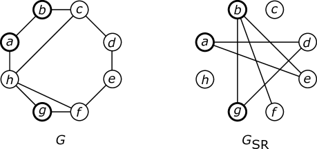
Figure 1: A Graph $G$ and its strong resolving graph ${G}_{\rm SR}$. The vertex set $\{\textsf{{a,b,g}}\}$ is a minimum vertex cover for ${G}_{\rm SR}$ and a minimum strong resolving set for $G$.

0.3 Composing graphs

The graphs we consider arise from attaching child graphs $G_{1},\ldots,G_{k}$ to a parent graph $H$. This attachment is performed by merging vertices $u_{1},\ldots,u_{k}$ of $G_{1},\ldots,G_{k}$ with vertices $v_{1},\ldots,v_{k}$ from $H$ in the disjoint union of the graphs $G_{1},\ldots,G_{k}$, and $H$.

Definition 1.

Let $G_{i}=(V_{i},E_{i})$, $1\leq i\leq k$, and $H=(V_{H},E_{H})$ be $k+1$ graphs, $u_{i}\in V_{i}$ for $i=1,\ldots,k$, and $v_{1},\ldots,v_{k}\in V_{H}$. Let $G_{1,\ldots,k}$ be the disjoint union of $G_{1},\ldots,G_{k}$. That is, $G_{1,\ldots,k}$ has vertex set $\cup_{i=1}^{k}V_{i}$ and edge set $\cup_{i=1}^{k}E_{i}$.

Then graph

$$G_{1,\ldots,k}{\,\circ_{(u_{1},\ldots,u_{k}\to v_{1},\ldots,v_{k})}\,}H$$

is defined by vertex set

$$(V_{1}\cup\cdots\cup V_{k}\cup V_{H})\setminus\{u_{1},\ldots,u_{k}\}$$

and edge set

$$\begin{array}[]{lll}(&E_{1}\cup\cdots\cup E_{k}\cup E_{H}&\\ &\cup\,\{\{w,v_{i}\}\,|\,w\in N_{G_{i}}(u_{i}),1\leq i\leq k\}&)\\ \setminus&\{\{w,u_{i}\}\,|\,w\in N_{G_{i}}(u_{i}),1\leq i\leq k\}.&\end{array}$$

The graph $G_{1,\ldots,k}{\,\circ_{(u_{1},\ldots,u_{k}\to v_{1},\ldots,v_{k})}\,}H$ is formed by the disjoint union of the $k$ graphs $G_{1},\ldots,G_{k}$ and graph $H$ without the vertices $u_{1},\ldots,u_{k}$ and their incident edges, in which for $i=1,\ldots,k$ the neighbours of vertex $u_{i}$ in $G_{i}$ are connected to vertex $v_{i}$. Figure 2 shows an example of the ${\,\circ_{(u_{1},\ldots,u_{k}\to v_{1},\ldots,v_{k})}\,}$ operation. For all further discussions, we only consider the case in that all graphs $G_{1},\ldots,G_{k},H$ are vertex disjoint, connected, and have at least two vertices. The vertices $v_{1},\ldots,v_{k}$ of $H$ do not need to be distinct.

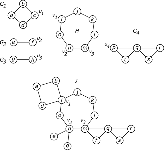
Figure 2: Five graphs $G_{1}$, $G_{2}$, $G_{3}$, $G_{4}$, $H$, and the graph $J=G_{1,2,3,4}{\,\circ_{(u_{1},u_{2},u_{3},u_{4}\to v_{1},v_{2},v_{2},v_{3})}\,}H$ created by the composition as defined in Definition 1.

0.4 The strong resolving graph

To compute a strong resolving set for a composed graph $J=G_{1,\ldots,k}{\,\circ_{(u_{1},\ldots,u_{k}\to v_{1},\ldots,v_{k})}\,}H$, we first determine the edge set of the strong resolving graph ${J}_{\rm SR}$.

Definition 2.

For a connected graph $G=(V,E)$ and a vertex $u\in V$, let ${\text{MD}(\,G,\,u\,)}$ be the set of vertices that are maximally distant from vertex $u$ in $G$.

The following prerequisite is used in each of the following lemmas and theorems.

Prerequisite 1.

Let $G_{i}=(V_{i},E_{i})$, $1\leq i\leq k$, and $H=(V_{H},E_{H})$ be $k+1$ vertex disjoint, connected graphs, $|V_{i}|\geq 2$, $u_{i}\in V_{i}$ for $i=1,\ldots,k$, $|V_{H}|\geq 2$, $v_{1},\ldots,v_{k}\in V_{H}$, let $G_{1,\ldots,k}$ be the disjoint union of $G_{1},\ldots,G_{k}$, and let

$$J=(V_{J},E_{J})=G_{1,\ldots,k}{\,\circ_{(u_{1},\ldots,u_{k}\to v_{1},\ldots,v_{k})}\,}H.$$

The vertices $v_{1},\ldots,v_{k}$ of $H$ do not need to be distinct.

Lemma 1.

Let 1 be given. Then the vertices $v_{1},\ldots,v_{k}$ have no incident edges in ${J}_{\rm SR}$.

Proof.

The vertices $v_{1},\ldots,v_{k}$ are separation vertices in $J$, because all graphs $G_{i}$, $1\leq i\leq k$, and $H$ are connected and have at least two vertices. Separation vertices are not maximally distant from any vertex. ∎

Lemma 2.

Let 1 be given. Let $w\in V_{H}$, then

$$\begin{array}[]{ll}{\text{MD}(\,J,\,w\,)}=&\left(\begin{array}[]{ll}&{\text{MD}(\,H,\,w\,)}\setminus\{v_{1},\ldots,v_{k}\}\\ \cup&\bigcup_{1\leq i\leq k}{\text{MD}(\,G_{i},\,u_{i}\,)}\end{array}\right).\end{array}$$

Proof.

This follows from the fact that each shortest path in $J$ between $w$ and a vertex of $G_{i}$ for $1\leq i\leq k$ passes vertex $v_{i}$ and each shortest path in $J$ between $w$ and a vertex of $H$ does not pass a vertex outside of $H$. Separation vertices are not maximally distant from any vertex, see also Lemma 1. ∎

In Figure 2 the vertices $\{\textsf{{a,o,e,g,t,s,r}}\}$ are maximally distant from vertex l in $J$.

Lemma 3.

Let 1 be given. Let $u^{\prime}_{j}\in V_{j}\setminus\{u_{j}\}$ for some $j$, $1\leq j\leq k$. Then

$$\begin{array}[]{ll}{\text{MD}(\,J,\,u^{\prime}_{j}\,)}=&\left(\begin{array}[]{ll}&{\text{MD}(\,G_{j},\,u^{\prime}_{j}\,)}\setminus\{u_{j}\}\\ \cup&{\text{MD}(\,H,\,v_{j}\,)}\setminus\{v_{1},\ldots,v_{k}\}\\ \cup&\bigcup_{1\leq i\leq k,i\not=j}{\text{MD}(\,G_{i},\,u_{i}\,)}\end{array}\right).\end{array}$$

Proof.

This follows from the fact that each shortest path in $J$ between $u^{\prime}_{j}$ and a vertex of $H$ or $G_{i}$ for $i\not=j$ passes vertex $v_{j}$ and each shortest path in $J$ between $u^{\prime}_{j}$ and a vertex of $(V_{j}\setminus\{u_{j}\})\cup\{v_{j}\}$ do not pass a vertex outside of $(V_{j}\setminus\{u_{j}\})\cup\{v_{j}\}$. Separation vertices are not maximally distant from any vertex, see also Lemma 1. Note that vertex $u_{j}$ can be maximally distant from $u^{\prime}_{j}$ in $G_{j}$, but is not a vertex of $J$. This is why we need to remove $u_{j}$ as well from ${\text{MD}(\,G_{j},\,u^{\prime}_{j}\,)}$. ∎

In Figure 2 the vertices $\{\textsf{{l,e,g,t,s,r}}\}$ are maximally distant from vertex a in $J$. Note that vertex c is also maximally distant from vertex a in $G_{1}$, but is excluded from ${\text{MD}(\,G_{1},\,\textsf{{a}}\,)}$.

The next lemmas characterise the edges of ${J}_{\rm SR}$ between vertices of $V_{i}\setminus\{u_{i}\}$ and vertices of $V_{j}\setminus\{u_{j}\}$ for $i\neq j$, and the edges between vertices of $V_{i}\setminus\{u_{i}\}$ and vertices of $V_{H}$.

Lemma 4.

Let 1 be given. Then for each vertex $u^{\prime}_{i}\in V_{i}\setminus\{u_{i}\}$ for some $i$, $1\leq i\leq k$, and each vertex $v^{\prime}\in V_{J}\setminus V_{i}$, the following statements hold true.

1. If $u^{\prime}_{i}$ is maximally distant from $u_{i}$ in $G_{i}$, or equivalently maximally distant from $v_{i}$ in $J$, then $u^{\prime}_{i}$ is maximally distant from $v^{\prime}$ in $J$.

2. If $v^{\prime}$ is maximally distant from $v_{i}$ in $J$, then $v^{\prime}$ is maximally distant from $u^{\prime}_{i}$ in $J$.

Proof.

This follows again from the fact that each shortest path in $J$ between $u^{\prime}_{i}$ and $v^{\prime}$ passes vertex $v_{i}$, and thus $d_{J}(u^{\prime}_{i},v^{\prime})=d_{J}(u^{\prime}_{i},v_{i})+d_{J}(v_{i},v^{\prime})$. ∎

In Figure 2 vertex a is maximally distant from vertex c in $G_{1}$, thus vertex a is maximally distant from all vertices except for b and d in $J$. Also, vertex e is maximally distant from vertex f in $G_{2}$, thus the vertices a and e are mutually maximally distant in $J$.

Lemma 5.

Let 1 be given. Two vertices $u^{\prime}_{i}\in V_{i}\setminus\{u_{i}\}$ and $u^{\prime}_{j}\in V_{j}\setminus\{u_{j}\}$ for $i\not=j$ are mutually maximally distant in $J$ if and only if $u^{\prime}_{i}$ is maximally distant from $u_{i}$ in $G_{i}$ and $u^{\prime}_{j}$ is maximally distant from $u_{j}$ in $G_{j}$.

Proof.

”$\Rightarrow$” Let $u^{\prime}_{i}$ be maximally distant from $u_{i}$ in $G_{i}$ and $u^{\prime}_{j}$ be maximally distant from $u_{j}$ in $G_{j}$. By Lemma 4, $u^{\prime}_{i}$ is maximally distant from each vertex of $V_{J}\setminus V_{i}$ and $u^{\prime}_{j}$ is maximally distant to each vertex of $V_{J}\setminus V_{j}$. Thus $u^{\prime}_{i}$ and $u^{\prime}_{j}$ are mutually maximally distant in $J$ and $\{u^{\prime}_{i},u^{\prime}_{j}\}$ is an edge in ${J}_{\rm SR}$.

”$\Leftarrow$” Since each path between $u^{\prime}_{i}$ and $u^{\prime}_{j}$ in $J$ passes vertex $u_{i}$ (and vertex $u_{j}$), the following statement holds true. If $u^{\prime}_{i}$ and $u^{\prime}_{j}$ are mutually maximally distant in $J$, then $u^{\prime}_{i}$ is maximally distant from $u_{i}$ in $G_{i}$ and $u^{\prime}_{j}$ is maximally distant from $u_{j}$ in $G_{j}$. ∎

Lemma 5 identifies the edges of ${J}_{\rm SR}$ between $u^{\prime}_{i}\in V_{i}$ and $u^{\prime}_{j}\in V_{j}$ for $i\neq j$.

Next we identify the edges of ${J}_{\rm SR}$ between two vertices of $V_{i}\setminus\{u_{i}\}$ and between two vertices of $V_{H}\setminus\{v_{1},\ldots,v_{k}\}$.

Lemma 6.

Let 1 be given.

1. Two vertices $u^{\prime}_{i},u^{\prime\prime}_{i}\in V_{i}\setminus\{u_{i}\}$ are mutually maximally distant in $J$ if and only if they are mutually maximally distant in $G_{i}$.

2. Two vertices $v^{\prime},v^{\prime\prime}\in V_{H}\setminus\{v_{1},\ldots,v_{k}\}$ are mutually maximally distant in $J$ if and only if they are mutually maximally distant in $H$.

Proof.

The statements follow from the facts that each shortest path between $u^{\prime}_{i}$ and $u^{\prime\prime}_{i}$ in $J$ does not pass a vertex of $V_{J}\setminus(V_{i}\cup\{v_{i}\})$ and each shortest path between $v^{\prime}$ and $v^{\prime\prime}$ in $J$ does not pass a vertex of $V_{1}\cup\ldots\cup V_{k}$. ∎

The following theorem follows from Lemma 5 and Lemma 6 and characterises all edges of ${J}_{\rm SR}$. Figure 3 shows the strong resolving graph ${J}_{\rm SR}$ of $J$ from Figure 2.

Theorem 1.

Let 1 be given. The strong resolving graph ${J}_{\rm SR}$ has an edge $\{w_{1},w_{2}\}$ if and only if $w_{1},w_{2}\notin\{v_{1},\ldots,v_{k}\}$ and

1. $w_{1},w_{2}\in V_{i}$ for some $i$, $1\leq i\leq k$, and $w_{1}$ and $w_{2}$ are mutually maximally distant in $G_{i}$,

2. $w_{1},w_{2}\in V_{H}$ and $w_{1}$ and $w_{2}$ are mutually maximally distant in $H$,

3. $w_{1}\in V_{i}$ and $w_{2}\in V_{j}$ for some $i,j$, $1\leq i<j\leq k$, and $w_{1}$ is maximally distant from $u_{i}$ in $G_{i}$ and $w_{2}$ is maximally distant from $u_{j}$ in $G_{j}$, or

4. if $w_{1}\in V_{i}$ for some $i$, $1\leq i\leq k$, $w_{2}\in V_{H}$, $w_{1}$ is maximally distant from $u_{i}$ in $G_{i}$ and $w_{2}$ is maximally distant from $v_{i}$ in $H$.

0.5 A minimum vertex cover

Theorem 1 characterises the edges in the strong resolving graph ${J}_{\rm SR}$ as follows, see Figure 3.

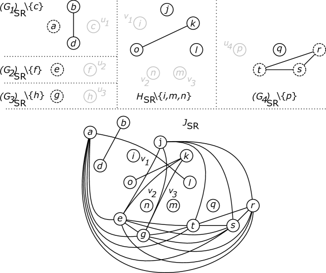
Figure 3: The graphs ${(G_{1})}_{\rm SR}\setminus\{\textsf{{c}}\}$, ${(G_{2})}_{\rm SR}\setminus\{\textsf{{f}}\}$, ${(G_{3})}_{\rm SR}\setminus\{\textsf{{h}}\}$, ${(G_{4})}_{\rm SR}\setminus\{\textsf{{p}}\}$, ${H}_{\rm SR}\setminus\{\textsf{{i,m,n}}\}$, and ${J}_{\rm SR}$, where $G_{1}$, $G_{2}$, $G_{3}$, $G_{4}$, $H$, and $J$ are from Figure 2. The dashed vertices in ${(G_{1})}_{\rm SR}$, ${(G_{2})}_{\rm SR}$, ${(G_{3})}_{\rm SR}$, and ${(G_{4})}_{\rm SR}$ are the vertices which are maximally distant from $u_{1}$, $u_{2}$, $u_{3}$, and $u_{4}$ in $G_{1}$, $G_{2}$, $G_{3}$, and $G_{4}$, respectively. The grey vertices are the vertices that are merged to separation vertices of $J$. These vertices are not taken into account when computing minimum strongly resolving sets for $J$.

• The edges considered in Case 1 are the edges of ${(G_{i})}_{\rm SR}\setminus\{u_{i}\}$.

• The edges considered in Case 2 are the edges of ${H}_{\rm SR}\setminus\{v_{1},\ldots,v_{k}\}$.

• The edges considered in Case 3 are the edges of a complete $k$-partite graph $K_{n_{1},\ldots,n_{k}}$, $n_{i}=|{\text{MD}(\,G_{i},\,u_{i}\,)}|$, with vertex set

  $$\bigcup_{1\leq i\leq k}{\text{MD}(\,G_{i},\,u_{i}\,)}$$

  and edge set

  $$\{\{w_{1},w_{2}\}\,|\,w_{1},\in{\text{MD}(\,G_{i},\,u_{i}\,)},w_{2},\in{\text{MD}(\,G_{j},\,u_{j}\,)},1\leq i<j\leq k\},$$

  .

• The edges considered in Case 4 are the edges of $k$ complete bipartite graphs $K_{n_{i},m_{i}}$, $1\leq i\leq k$, $n_{i}=|{\text{MD}(\,G_{i},\,u_{i}\,)}|$, $m_{i}=|{\text{MD}(\,H,\,v_{i}\,)}\setminus\{v_{1},\ldots,v_{k}\}|$ with vertex set

  $${\text{MD}(\,G_{i},\,u_{i}\,)}\,\cup\,(\,{\text{MD}(\,H,\,v_{i}\,)}\setminus\{v_{1},\ldots,v_{k}\}\,)$$

  and edge set

  $$\{\{w_{1},w_{2}\}\,|\,w_{1},\in{\text{MD}(\,G_{i},\,u_{i}\,)},w_{2},\in{\text{MD}(\,H,\,v_{i}\,)}\setminus\{v_{1},\ldots,v_{k}\}\}.$$

As mentioned in Section 0.2, a vertex set is a strong resolving set for $J$ if and only if it is a vertex cover for ${J}_{\rm SR}$. The strong resolving graph ${J}_{\rm SR}$ contains the $k$-partite graph $K_{n_{1},\ldots,n_{k}}$ and the $k$ bipartite graphs $K_{n_{i},m_{i}}$, $1\leq i\leq k$, as subgraphs. That is, each vertex cover $U$ for ${J}_{\rm SR}$ contains for some $j$, $1\leq j\leq k$, all vertices of the vertex sets ${\text{MD}(\,G_{i},\,u_{i}\,)}$, $1\leq i\leq k$, $i\neq j$, and additionally either all vertices of ${\text{MD}(\,G_{j},\,u_{j}\,)}$ or all vertices of ${\text{MD}(\,H,\,v_{j}\,)}\setminus\{v_{1},\ldots,v_{k}\}$.

To compute the size of a minimum vertex cover of ${J}_{\rm SR}$, we use the following notation of a restricted vertex cover.

Notation 1.

For a graph $G=(V,E)$ let

$${\text{VC}(\,G\,)}$$

be a minimum vertex cover for $G$. For a graph $G=(V,E)$ and a vertex set $M\subseteq V$ let

$${\overline{\text{VC}}(\,G,\,M\,)}$$

be a vertex set of minimum size that contains all vertices of $M$ and which is a vertex cover for $G$.

With the help of 1, a minimum vertex cover for ${J}_{\rm SR}$ can now easily be specified.

Lemma 7.

Let 1 be given. Let

$$U_{0}=\left(\begin{array}[]{ll}&{\text{VC}(\,{H}_{\rm SR}\setminus\{v_{1},\ldots,v_{k}\}\,)}\\ \cup&\bigcup_{1\leq i\leq k}{\overline{\text{VC}}(\,{(G_{i})}_{\rm SR}\setminus\{u_{i}\},\,{\text{MD}(\,G_{i},\,u_{i}\,)}\,)}\end{array}\right)$$

and

$$U_{j}=\left(\begin{array}[]{ll}&{\overline{\text{VC}}(\,{H}_{\rm SR}\setminus\{v_{1},\ldots,v_{k}\},\,{\text{MD}(\,H,\,v_{j}\,)}\setminus\{v_{1},\ldots,v_{k}\}\,)}\\ \cup&{\text{VC}(\,{(G_{j})}_{\rm SR}\setminus\{u_{j}\}\,)}\\ \cup&\bigcup_{1\leq i\leq k,i\not=j}{\overline{\text{VC}}(\,{(G_{i})}_{\rm SR}\setminus\{u_{i}\},\,{\text{MD}(\,G_{i},\,u_{i}\,)}\,)}\end{array}\right)$$

for $j=1,\ldots,k$.

Each vertex sets $U_{0},U_{1},\ldots,U_{k}$ is a vertex cover for ${J}_{\rm SR}$, where at least one of them is a minimum vertex cover ${J}_{\rm SR}$.

Proof.

As mentioned above, ${J}_{\rm SR}$ contains a complete $k$-partite subgraph with vertex set

$${\text{MD}(\,G_{1},\,u_{1}\,)}\,\cup\,\cdots\,\cup\,{\text{MD}(\,G_{k},\,u_{k}\,)}$$

and $k$ bipartite subgraphs with vertex sets

$${\text{MD}(\,G_{i},\,u_{i}\,)}\,\cup\,({\text{MD}(\,H,\,u_{i}\,)}\setminus\{u_{1},\ldots,u_{k}\})$$

for $i=1,\ldots,k$. Each vertex cover of ${J}_{\rm SR}$ must therefore contain all vertices from all sets ${\text{MD}(\,G_{1},\,u_{1}\,)},\ldots,{\text{MD}(\,G_{k},\,u_{k}\,)}$ except for one of these sets ${\text{MD}(\,G_{j},\,u_{j}\,)}$, $1\leq j\leq k$, and must additionally contain either all vertices of ${\text{MD}(\,G_{j},\,u_{j}\,)}$ or all vertices of ${\text{MD}(\,H,\,v_{j}\,)}\setminus\{v_{1},\ldots,v_{k}\}$. The edges in ${J}_{\rm SR}$ which are not incident with the vertices of the selected sets must of course also be covered by a vertex cover. These $k+1$ cases are treated by considering the sets $U_{0},U_{1},\ldots,U_{k}$. ∎

The next two lemmas consider the case that graph $H$ has an additional vertex $w$ that can be used to attach $J$ to further graphs, see Figure 4.

Figure 4: The strong resolving graph ${J}_{\rm SR}$ without vertex $w$, where $G_{1}$, $G_{2}$, $G_{3}$, $G_{4}$, and $H$ are from Figure 2. The four vertex sets $\{\textsf{{a}}\}$, $\{\textsf{{e}}\}$, $\{\textsf{{g}}\}$, $\{\textsf{{r,s,t}}\}$ form a complete 4-partite subgraph of ${J}_{\rm SR}$. Vertex a is the only vertex that is maximally distant from $u_{1}$ in $G_{1}$, vertex e is the only vertex that is maximally distant from $u_{2}$ in $G_{2}$, vertex g is the only vertex that is maximally distant from $u_{3}$ in $G_{3}$, and the vertices r,s,t are the only vertices that are maximally distant from $u_{4}$ in $G_{4}$. Also, the vertices l and m are maximally distant from $v_{1}$, the vertices j and k are maximally distant from $v_{2}$, and the vertices i and j are maximally distant from $v_{3}$ in $H$. Therefore, the vertex sets $\{\textsf{{e}}\}$ and $\{\textsf{{j,k}}\}$ form a complete bipartite subgraph in ${J}_{\rm SR}$, the vertex sets $\{\textsf{{g}}\}$ and $\{\textsf{{j,k}}\}$ form a second complete bipartite subgraph and the vertex sets $\{\textsf{{r,s,t}}\}$ and $\{\textsf{{j}}\}$ form a third one. Since the vertices i,m and n are separation vertices in $J$ and the vertex l will be a separation vertex later on (see Lemma 8 and Lemma 9), they have no incident edges in ${J}_{\rm SR}$.

Lemma 8.

Let 1 be given and $w\in V_{H}$. Let

$$U_{0}=\left(\begin{array}[]{ll}&{\text{VC}(\,{H}_{\rm SR}\setminus\{v_{1},\ldots,v_{k},w\}\,)}\\ \cup&\bigcup_{1\leq i\leq k}{\overline{\text{VC}}(\,{(G_{i})}_{\rm SR}\setminus\{u_{i}\},\,{\text{MD}(\,G_{i},\,u_{i}\,)}\,)}\end{array}\right)$$

and

$$U_{j}=\left(\begin{array}[]{ll}&{\overline{\text{VC}}(\,{H}_{\rm SR}\setminus\{v_{1},\ldots,v_{k},w\},\,{\text{MD}(\,H,\,v_{j}\,)}\setminus\{v_{1},\ldots,v_{k},w\}\,)}\\ \cup&{\text{VC}(\,{(G_{j})}_{\rm SR}\setminus\{u_{j}\}\,)}\\ \cup&\bigcup_{1\leq i\leq k,i\not=j}{\overline{\text{VC}}(\,{(G_{i})}_{\rm SR}\setminus\{u_{i}\},\,{\text{MD}(\,G_{i},\,u_{i}\,)}\,)}\end{array}\right)$$

for $j=1,\ldots,k$.

Each vertex sets $U_{0},U_{1},\ldots,U_{k}$ is a vertex cover for ${J}_{\rm SR}\setminus\{w\}$, where at least one of them is a minimum vertex cover ${J}_{\rm SR}$.

Proof.

The only difference between Lemma 7 and Lemma 8 is the additional vertex $w$ in $H$, which is removed from the computations of the vertex covers, since it becomes a separation vertex in all further compositions. The correctness follows from the reasoning applied in Lemma 7. ∎

Lemma 9.

Let 1 be given and $w\in V_{H}$. Then

$$\left(\begin{array}[]{ll}&{\overline{\text{VC}}(\,{H}_{\rm SR}\setminus\{v_{1},\ldots,v_{k},w\},\,{\text{MD}(\,H,\,w\,)}\setminus\{v_{1},\ldots,v_{k},w\}\,)}\\ \cup&\bigcup_{1\leq i\leq k}{\overline{\text{VC}}(\,{(G_{i})}_{\rm SR}\setminus\{u_{i}\},\,{\text{MD}(\,G_{i},\,u_{i}\,)}\,)}.\end{array}\right)$$

is a minimum vertex cover for ${J}_{\rm SR}\setminus\{w\}$ that contains all vertices of ${\text{MD}(\,J,\,w\,)}$.

Proof.

A vertex cover for ${G}_{\rm SR}$ that additionally contains all vertices from the sets ${\text{MD}(\,G_{i},\,u_{i}\,)}$, $1\leq i\leq k$, already covers all edges of the k-partite graph and the $k$ bipartite graphs as defined in the proof of Lemma 7. Therefore, no further case distinctions are necessary for the computation of ${\overline{\text{VC}}(\,{J}_{\rm SR}\setminus\{w\},\,{\text{MD}(\,J,\,w\,)}\,)}$, based on Lemma 2. ∎

The results from Lemmas 7, 8 and 9 are summarized by the following theorem.

Theorem 2.

Let 1 be given and $w\in V_{H}$. Then

$${\text{VC}(\,{J}_{\rm SR}\,)},$$

$${\text{VC}(\,{J}_{\rm SR}\setminus\{w\}\,)},$$

and

$${\overline{\text{VC}}(\,{J}_{\rm SR}\setminus\{w\},\,{\text{MD}(\,J,\,w\,)}\,)}$$

are computable from $G_{1},\ldots,G_{k},H$, $u_{1},\ldots,u_{k}$, $v_{1},\ldots,v_{k}$, $w$, and the following vertex sets.

1. ${\text{VC}(\,{(G_{i})}_{\rm SR}\setminus\{u_{i}\}\,)}$, for $i=1,\ldots,k$,
   (used by Lemma 7: $U_{j}$, Lemma 8: $U_{j}$,),

2. ${\overline{\text{VC}}(\,{(G_{i})}_{\rm SR}\setminus\{u_{i}\},\,{\text{MD}(\,G_{i},\,\{u_{i}\}\,)}\,)}$ for $i=1,\ldots,k$,
   (used by Lemma 7: $U_{0}$, $U_{j}$, Lemma 8: $U_{0}$, $U_{j}$, Lemma 9),

3. 1. ${\text{VC}(\,{H}_{\rm SR}\setminus\{v_{1},\ldots,v_{k}\}\,)}$,
      (used by Lemma 7: $U_{0}$),

   2. ${\text{VC}(\,{H}_{\rm SR}\setminus\{v_{1},\ldots,v_{k},w\}\,)}$,
      (used by Lemma 8: $U_{0}$),

4. 1. ${\overline{\text{VC}}(\,{H}_{\rm SR}\setminus\{v_{1},\ldots,v_{k}\},\,{\text{MD}(\,H,\,\{v_{i}\}\,)}\setminus\{v_{1},\ldots,v_{k}\}\,)}$ for $i=1,\ldots,k$,
      (used by Lemma 7: $U_{j}$),

   2. ${\overline{\text{VC}}(\,{H}_{\rm SR}\setminus\{v_{1},\ldots,v_{k},w\},\,{\text{MD}(\,H,\,\{v_{i}\}\,)}\setminus\{v_{1},\ldots,v_{k},w\}\,)}$ for $i=1,\ldots,k$,
      (used by Lemma 8: $U_{j}$), and

5. ${\overline{\text{VC}}(\,{H}_{\rm SR}\setminus\{v_{1},\ldots,v_{k},w\},\,{\text{MD}(\,H,\,\{w\}\,)}\setminus\{v_{1},\ldots,v_{k},w\}\,)}$,
   (used by Lemma 9).

In the next section we show how a minimum strong resolving set for a graph $G$ can be efficiently computed using Lemmas 7, 8 and 9, provided that a minimum strong resolving set for the biconnected components can be efficiently computed.

0.6 The algorithmic frame

The given graph $G$ is first decomposed into its biconnected components. Edges, whose end vertices are separation vertices or vertices of degree one, are also regarded as biconnected components. Then the decomposition tree $T$ for $G$ is built. We use variable names with a hat symbol for nodes in trees to distinguish them from the vertices in graphs. Tree $T$ contains a so-called b-node for each biconnected component of $G$ and a so-called s-node for each separation vertex of $G$. A b-node $\hat{u}$ and an s-node $\hat{v}$ are connected by an edge $\{\hat{u},\hat{v}\}$ in $T$ if and only if the separation vertex for $\hat{v}$ is part of the biconnected component for $\hat{u}$. The preprocessing to compute $T$ can be done in linear time. Figure 5 shows an example of such a decomposition.

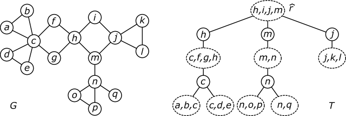
Figure 5: A graph $G$ to the left and its decomposition tree $T$ to the right. The dashed circles are the b-nodes of $T$ for the biconnected components of $G$. The other nodes are the s-nodes of $T$ for the separation vertices in $G$. The b-node for the biconnected component of $G$ induced by the vertices h,i,j,m has been selected as the root $\hat{r}$ of $T$.

Computing a minimum strong resolving set for $G$, or equivalently, computing a minimum vertex cover for ${G}_{\rm SR}$, can now be done via a bottom-up processing of $G$ according to the decomposition tree $T$. Tree $T$ is first oriented by choosing any b-node $\hat{r}$ of $T$ as the root of $T$. All leaves of $T$ are b-nodes. The predecessor nodes of the leaves are s-nodes for separation vertices of $G$ that connect the biconnected components of the leafs to the rest of $G$. The predecessor nodes of the predecessor nodes of the leaves of $T$ are again b-nodes for biconnected components of $G$ at which the biconnected components for the leaves are linked via the separation vertices, and so on.

For a b-node $\hat{u}$ of $T$ let $G(\hat{u})$ be the biconnected component for $\hat{u}$ and $\widetilde{G}(\hat{u})$ be the subgraph of $G$ induced by the vertices of all biconnected components of the b-nodes in the subtree of $T$ with root $\hat{u}$. For an s-node $\hat{v}$ let ${\rm s}(\hat{v})$ be the separation vertex for $\hat{v}$.

A minimum strong resolving set for $G$ is equal to ${\text{VC}(\,{\widetilde{G}(\hat{r})}_{\rm SR}\,)}$, which can be calculated based on informations about $G(\hat{r})$ and the subgraphs attached to it, using Lemmas 7, 8 and 9.

To describe the vertex sets we calculate more detailed, we consider the following cases. Let $\hat{u}$ be a b-node of $T$.

1. If $\hat{u}$ is a leaf with predecessor s-node $\hat{w}$, then we calculate the two sets

   $${\text{VC}(\,{\widetilde{G}(\hat{u})}_{\rm SR}\setminus\{{\rm s}(\hat{w})\}\,)}\quad\text{and}\quad{\overline{\text{VC}}(\,{\widetilde{G}(\hat{u})}_{\rm SR}\setminus\{{\rm s}(\hat{w})\},\,{\text{MD}(\,\widetilde{G}(\hat{u}),\,{\rm s}(\hat{w})\,)}\,)}$$

   directly from the biconnected subgraph $\widetilde{G}(\hat{u})=G(\hat{u})$ of $G$. Figure 6 shows an example of this case on the left-hand side. If $\hat{u}$ is a leaf without a predecessor s-node, then $G(\hat{u})=G$ and we calculate ${\text{VC}(\,{G(\hat{u})}_{\rm SR}\,)}$ directly.

2. If $\hat{u}$ is an inner b-node of $T$ with predecessor s-node $\hat{w}$, let $\hat{u}_{1},\cdots,\hat{u}_{k}$ be the successor b-nodes of the successor s-nodes of $\hat{u}$, and $\hat{v}_{1},\ldots,\hat{v}_{k}$ be the predecessor s-nodes of $\hat{u}_{1},\cdots,\hat{u}_{k}$. Note that $\hat{v}_{1},\ldots,\hat{v}_{k}$ do not need to be distinct. Figure 6 shows an example of this case on the right-hand side. If we replace the separation vertex ${\rm s}(\hat{v}_{i})$ in subgraph $\widetilde{G}(\hat{u}_{i})$ by a new vertex $w_{i}$ such that all $k$ graphs $\widetilde{G}(\hat{u}_{1}),\ldots,\widetilde{G}(\hat{u}_{k})$, and the biconnected component $G(\hat{u})$ are vertex-disjoint, then

   $$\widetilde{G}(\hat{u})=(\widetilde{G}(\hat{u}_{1})\cup\ldots\cup\widetilde{G}(\hat{u}_{k})){\,\circ_{(w_{1},\ldots,w_{k}\to{\rm s}(\hat{v}_{1}),\ldots,{\rm s}(\hat{v}_{k}))}\,}G(\hat{u}).$$

   We then calculate the two sets

   $${\text{VC}(\,{\widetilde{G}(\hat{u})}_{\rm SR}\setminus\{{\rm s}(\hat{w})\}\,)}\quad\text{and}\quad{\overline{\text{VC}}(\,{\widetilde{G}(\hat{u})}_{\rm SR}\setminus\{{\rm s}(\hat{w})\},\,{\text{MD}(\,\widetilde{G}(\hat{u}),\,{\rm s}(\hat{w})\,)}\,)}$$

   using Lemmas 8 and 9. Those lemmas require the vertex sets
   ${\text{VC}(\,{G(\hat{u})}_{\rm SR}\setminus\{{\rm s}(\hat{v}_{1}),\ldots,{\rm s}(\hat{v}_{k}),{\rm s}(\hat{w})\}\,)}$,
   ${\overline{\text{VC}}(\,{G(\hat{u})}_{\rm SR}\setminus\{{\rm s}(\hat{v}_{1}),\ldots,{\rm s}(\hat{v}_{k}),{\rm s}(\hat{w})\},\,{\text{MD}(\,G(\hat{u}),\,{\rm s}(\hat{v}_{i})\,)}\setminus\{{\rm s}(\hat{v}_{1}),\ldots,{\rm s}(\hat{v}_{k}),{\rm s}(\hat{w})\}\,)}$, and
   ${\overline{\text{VC}}(\,{G(\hat{u})}_{\rm SR}\setminus\{{\rm s}(\hat{v}_{1}),\ldots,{\rm s}(\hat{v}_{k}),{\rm s}(\hat{w})\},\,{\text{MD}(\,G(\hat{u}),\,{\rm s}(\hat{w})\,)}\setminus\{{\rm s}(\hat{v}_{1}),\ldots,{\rm s}(\hat{v}_{k}),{\rm s}(\hat{w})\}\,)}$.

3. If $\hat{u}=\hat{r}$, then we calculate the set

   $${\text{VC}(\,{\widetilde{G}(\hat{u})}_{\rm SR}\,)}$$

   using Lemma 7. This lemma requires the vertex sets
   ${\text{VC}(\,{G(\hat{u})}_{\rm SR}\setminus\{{\rm s}(\hat{v}_{1}),\ldots,{\rm s}(\hat{v}_{k})\}\,)}$ and
   ${\overline{\text{VC}}(\,{G(\hat{u})}_{\rm SR}\setminus\{{\rm s}(\hat{v}_{1}),\ldots,{\rm s}(\hat{v}_{k})\},\,{\text{MD}(\,G(\hat{u}),\,{\rm s}(\hat{v}_{i})\,)}\setminus\{{\rm s}(\hat{v}_{1}),\ldots,{\rm s}(\hat{v}_{k})\}\,)}$.

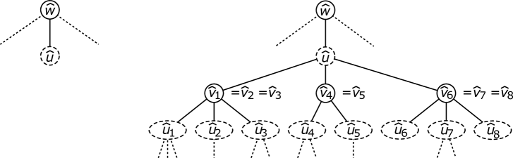
Figure 6: The left-hand side shows the first case where the b-node $\hat{u}$ is a leaf of $T$. The right-hand side shows the second case in which the b-node $\hat{u}$ is an inner node of $T$.

Recall that Lemmas 7 and 8 focus on the $k$ bipartite subgraphs of ${\widetilde{G}(\hat{u})}_{\rm SR}$ (formerly ${J}_{\rm SR}$), between vertices of $\widetilde{G}(\hat{u}_{i})$ (formerly $G_{i}$) and vertices of $G(\hat{u})$ (formerly $H$). To determine which one of those $k$ bipartite subgraphs, if any, needs to be covered by vertices of $G(\hat{u})$, we defined the sets $U_{j}$ for $0\leq j\leq k$. The sizes of those sets can be calculated as follow. Note that we focus on Lemma 8, since Lemma 7 is only needed for the root $\hat{r}$, with the only difference being the separation vertex $s(\hat{w})$. Let

$$h_{i}=|{\overline{\text{VC}}(\,{G(\hat{u})}_{\rm SR}\setminus\{{\rm s}(\hat{v}_{1}),\ldots,{\rm s}(\hat{v}_{k}),{\rm s}(\hat{w})\},\,{\text{MD}(\,G(\hat{u}),\,{\rm s}(\hat{v}_{i})\,)}\setminus\{{\rm s}(\hat{v}_{1}),\ldots,{\rm s}(\hat{v}_{k}),{\rm s}(\hat{w})\}\,)}|$$

and let

$$h^{\prime}_{i}=|{\overline{\text{VC}}(\,{\widetilde{G}(\hat{u}_{i})}_{\rm SR}\setminus\{{\rm s}(\hat{v}_{i})\},\,{\text{MD}(\,\widetilde{G}(\hat{u}_{i}),\,{\rm s}(\hat{v}_{i})\,)}\,)}|.$$

Then $h_{i}$ is the number of vertices needed to cover the $i$-th bipartite subgraph with vertices of $G(\hat{u})$ and $h^{\prime}_{i}$ is the number of vertices needed to cover it with vertices of $\widetilde{G}(\hat{u}_{i})$. Therefore, $|U_{i}|=|U_{0}|+h_{i}-h^{\prime}_{i}$ for $1\leq i\leq k$.

The previous considerations mainly come down to the following. To compute the strong metric dimension of a graph based on the biconnected components, the size of
${\overline{\text{VC}}(\,{H}_{\rm SR}\setminus W,\,{\text{MD}(\,H,\,u\,)}\setminus W\,)}$ for a given graph $H$, a vertex $u$ of $H$, and a vertex set $W$ of $H$ has to be determined. If this size can be calculated in total linear (respectively polynomial) time for $k$ different vertices $u$ for an integer $i$ and a (possibly empty) vertex set $W$ for every biconnected component $H$, it is generally possible to compute the strong metric dimension of the whole graph in total linear (respectively polynomial) time as well. Therefore the total running time of the entire computation depends on the computations of the minimum vertex covers for the induced subgraphs ${G(\hat{u})}_{\rm SR}$ of the b-nodes $\hat{u}$ of $T$, as well as the modified vertex covers including the vertices, which are maximally distant from the separation vertices. In the next section we explain the processing time in more detail using three examples.

0.7 Three examples

Let again $\hat{u}$, $\hat{u}_{1},\ldots,\hat{u}_{k}$ be b-nodes of $T$ and $\hat{w}$, $\hat{v}_{1},\ldots,\hat{v}_{k}$ be the predecessor s-nodes of them in the manner they are used in Section 0.6, see also Figure 6 on the right. The following examples show how to compute

• ${\text{VC}(\,{\widetilde{G}(\hat{u})}_{\rm SR}\,)}$,

• ${\text{VC}(\,{\widetilde{G}(\hat{u})}_{\rm SR}\setminus\{{\rm s}(\hat{w})\}\,)}$, and

• ${\overline{\text{VC}}(\,{\widetilde{G}(\hat{u})}_{\rm SR}\setminus\{{\rm s}(\hat{w})\},\,{\text{MD}(\,\widetilde{G}(\hat{u}),\,{\rm s}(\hat{w})\,)}\,)}$

in linear time if the biconnected components have a specific structure. In order to compute the sets above in linear time, we show

1. how to compute

   $${\overline{\text{VC}}(\,{G(\hat{u}_{i})}_{\rm SR}\setminus\{{\rm s}(\hat{v}_{1}),\ldots,{\rm s}(\hat{v}_{k}),{\rm s}(\hat{w})\},\,{\text{MD}(\,G(\hat{u}_{i}),\,{\rm s}(\hat{w})\,)}\setminus\{{\rm s}(\hat{v}_{1}),\ldots,{\rm s}(\hat{v}_{k}),{\rm s}(\hat{w})\}\,)}$$

   in linear time and

2. how to decide which of the sets $U_{0},U_{1},\ldots,U_{k}$ from Lemmas 8 and 9 is the smallest set in total linear time.

0.7.1 Grids

As our first example we consider grids. Let $G$ be an $n\times m$ grid with vertex set

$$\{x_{1,1},\ldots,x_{1,m},\ldots,x_{n,1},\ldots,x_{n,m}\},$$

with $n,m\geq 2$. The strong resolving graph of $G$ only contains the two edges $\{x_{1,1},x_{n,m}\}$ and $\{x_{1,m},x_{n,1}\}$. Therefore, computing a vertex cover for ${G}_{\rm SR}$ is fairly simple and ${\text{MD}(\,G,\,x_{i,j}\,)}$ can be determined easily as well.

Observation 1.

Let $G$ be an $n\times m$ grid as defined above and let $x_{i,j}$ with $1\leq i\leq n$ and $1\leq j\leq m$ be a vertex of $G$.

1. If $i\in\{1,n\}$ and $j\in\{1,m\}$, then ${\text{MD}(\,G,\,x_{i,j}\,)}=\{x_{n+1-i,m+1-j}\}$. That is, if $x_{i,j}$ is a corner vertex of the grid, then ${\text{MD}(\,G,\,x_{i,j}\,)}$ only contains the opposite corner vertex.

2. If $i\in\{1,n\}$ and $j\notin\{1,m\}$, then ${\text{MD}(\,G,\,x_{i,j}\,)}=\{x_{n+1-i,1},x_{n+1-i,m}\}$. Analogously, if $i\notin\{1,n\}$ and $j\in\{1,m\}$, then ${\text{MD}(\,G,\,x_{i,j}\,)}=\{x_{1,m+1-j},x_{n,m+1-j}\}$. That is, if $x_{i,j}$ is an edge vertex of the grid, then ${\text{MD}(\,G,\,x_{i,j}\,)}$ contains the two corner vertices on the opposite edge.

3. If $i\notin\{1,n\}$ and $j\notin\{1,m\}$, then ${\text{MD}(\,G,\,x_{i,j}\,)}=\{x_{1,1},x_{n,1},x_{1,m},x_{n,m}\}$. That is, if $x_{i,j}$ is an inner vertex of the grid, then ${\text{MD}(\,G,\,x_{i,j}\,)}$ contains all four corner vertices.

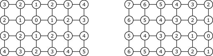
Figure 7: A grid $G_{4,6}$ and the distance of each vertex from the inner vertex $x_{2,3}$ on the left, and from the edge vertex $x_{3,6}$ on the right. This example illustrates the distribution of distances in a grid, that only corner vertices are maximally distant from other vertices, and which corner vertices those are for different types of vertex in the grid.

Figure 7 shows an example of a $4\times 6$ grid and the distances of the vertices to illustrate the previous observation. Since ${G}_{\rm SR}$ only contains two edges as mentioned above and with the previous observation, it is straight forward to see, that the size of ${\overline{\text{VC}}(\,{G}_{\rm SR}\setminus W,\,{\text{MD}(\,G,\,x_{i,j}\,)}\setminus W\,)}$ can be calculated in constant time for every vertex $x_{i,j}$ and an arbitrary vertex set $W$ if the position of each vertex inside the grid is known. Therefore, the following theorem follows.

Theorem 3.

A minimum strong resolving set for a graph $G=(V,E)$, in that each biconnected component is a grid, can be computed in time ${\mathcal{O}}(|V|+|E|)$.

0.7.2 Cycles

Consider the example in which each biconnected component $G(\hat{u})$ of $G$ is a cycle with at least three vertices $x_{0},x_{1},\ldots,x_{n-1}$, $n\geq 3$. The edge set of $G(\hat{u})$ is

$$\{\{x_{0},x_{1}\},\{x_{1},x_{2}\},\ldots,\{x_{n-1},x_{0}\}\}.$$

If $n$ is even, then ${G(\hat{u})}_{\rm SR}$ consists of $n/2$ edges, such that no two edges have a vertex in common. In this case, ${\text{MD}(\,G(\hat{u}),\,x_{i}\,)}$ contains the single vertex $x_{j}$ with $j=(i+n/2)\bmod n$. If $n$ is odd, then ${G(\hat{u})}_{\rm SR}$ is a cycle and ${\text{MD}(\,G(\hat{u}),\,x_{i}\,)}$ contains the two vertices $x_{j}$ and $x_{j+1}$ with $j=(i+\lfloor n/2\rfloor)\bmod n$, see Figure 8 for an example.

In both cases, ${G(\hat{u})}_{\rm SR}\setminus\{{\rm s}(\hat{v}_{1}),\ldots,{\rm s}(\hat{v}_{k}),{\rm s}(\hat{w})\}$ is a collection of paths. A minimum vertex cover of

$${G(\hat{u})}_{\rm SR}\setminus\{{\rm s}(\hat{v}_{1}),\ldots,{\rm s}(\hat{v}_{k}),{\rm s}(\hat{w})\}$$

has $\lfloor l/2\rfloor$ vertices from each path of those paths with $l$ vertices. However,

$${\overline{\text{VC}}(\,{G(\hat{u})}_{\rm SR}\setminus\{{\rm s}(\hat{v}_{1}),\ldots,{\rm s}(\hat{v}_{k}),{\rm s}(\hat{w})\},\,{\text{MD}(\,G(\hat{u}),\,x_{i}\,)}\setminus\{{\rm s}(\hat{v}_{1}),\ldots,{\rm s}(\hat{v}_{k}),{\rm s}(\hat{w})\}\,)}$$

may have some additional vertices depending on which paths the vertices from ${\text{MD}(\,G(\hat{u}),\,x_{i}\,)}$ belong to. Since ${\text{MD}(\,G(\hat{u}),\,x_{i}\,)}$ contains at most two vertices, the size of

$${\overline{\text{VC}}(\,{G(\hat{u})}_{\rm SR}\setminus\{{\rm s}(\hat{v}_{1}),\ldots,{\rm s}(\hat{v}_{k}),{\rm s}(\hat{w})\},\,{\text{MD}(\,G(\hat{u}),\,x_{i}\,)}\setminus\{{\rm s}(\hat{v}_{1}),\ldots,{\rm s}(\hat{v}_{k}),{\rm s}(\hat{w})\}\,)}$$

can easily be computed in constant time. Here the length of the paths on which the vertices are located, and in addition, if both vertices are located on the same path $p$, the distance between them on $p$ must be taken into account. Also observe, that the vertices of ${\text{MD}(\,G(\hat{u}),\,x_{i}\,)}$ are always at the end of paths if $x_{i}$ is one of the vertices which are removed from ${G(\hat{u})}_{\rm SR}$.

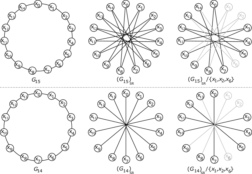
Figure 8: Two circles of 15 and 14 vertices on the left, the corresponding strong resolving graphs ${(G_{15})}_{\rm SR}$ and ${(G_{14})}_{\rm SR}$ in the middle, and the strong resolving graphs without the vertices $x_{1},x_{2},x_{6}$ on the right.

Overall the size of ${\overline{\text{VC}}(\,{H}_{\rm SR}\setminus W,\,{\text{MD}(\,H,\,u\,)}\setminus W\,)}$ for $k$ different vertices $u$ and a vertex set $W$ can be computed in total linear time if $H$ is a cycle. Thus, all calculations required to determine the strong metric dimension of $G$ can be done in total linear time if all biconnected components of $G$ are cycles, using the algorithm from Section 0.6. Also, which of the sets $U_{0},U_{1},\ldots,U_{k}$ is the smallest can be determined using the values $h_{i}$ and $h^{\prime}_{i}$ mentioned at the end of Section 0.6.

Theorem 4.

A minimum strong resolving set for a graph $G=(V,E)$, in that each biconnected component is a cycle, can be computed in time ${\mathcal{O}}(|V|+|E|)$.

0.7.3 Co-Graphs

A more complex example arises if each biconnected component $G(\hat{u})$ of $G$ is a co-graph. Co-graphs can be defined as follows.

Definition 3 (Co-Graphs and Co-Trees).

[CLB81]

• A graph $G$ that consists of a single vertex $u$ is a co-graph. The co-tree $T$ for $G$ consists of a single node $\hat{u}$ associated with vertex $u$ of $G$. Node $\hat{u}$ is the root of $T$. Let ${\rm vertex}(\hat{u})=u$ and ${\rm node}(u)=\hat{u}$. Note that ${\rm vertex}(\hat{u})$ is only defined for leaves $\hat{u}$ of $T$.

• If $G_{1}=(V_{1},E_{1})$ and $G_{2}=(V_{2},E_{2})$ are two co-graphs, then the disjoint union of $G_{1}$ and $G_{2}$, denoted by $G_{1}\hbox{\small$\cup$}\,G_{2}$, is a co-graph $G$ with vertex set $V_{1}\cup V_{2}$ and edge set $E_{1}\cup E_{2}$. Let $T_{1}$ and $T_{2}$ be co-trees for $G_{1}$ and $G_{2}$ with root $\hat{u}_{1}$ and $\hat{u}_{2}$, respectively. Then tree $T$ defined by the disjoint union of $T_{1}$ and $T_{2}$ with an additional node $\hat{u}$ and two additional edges $\{\hat{u},\hat{u}_{1}\}$ and $\{\hat{u},\hat{u}_{2}\}$ is a co-tree for $G$. Node $\hat{u}$ is the root of $T$ labelled by $\cup$ . Node $\hat{u}_{1}$ and $\hat{u}_{2}$ are successor nodes of $\hat{u}$. Node $\hat{u}$ is the predecessor node of $\hat{u}_{1}$ and $\hat{u}_{2}$.

• If $G_{1}=(V_{1},E_{1})$ and $G_{2}=(V_{2},E_{2})$ are two co-graphs, then the join of $G_{1}$ and $G_{2}$, denoted by $G_{1}\hbox{$\times$}\,G_{2}$, is a co-graph with vertex set $V_{1}\cup V_{2}$ and edge set $E_{1}\cup E_{2}\cup\{\{u,v\}\ |\ u\in V_{1},v\in V_{2}\}$. Let $T_{1}$ and $T_{2}$ be co-trees for $G_{1}$ and $G_{2}$ with root $\hat{u}_{1}$ and $\hat{u}_{2}$, respectively. Then tree $T$ defined by the disjoint union of $T_{1}$ and $T_{2}$ with an additional node $\hat{u}$ and two additional edges $\{\hat{u},\hat{u}_{1}\}$ and $\{\hat{u},\hat{u}_{2}\}$ is a co-tree for $G$. Node $\hat{u}$ is the root of $T$ labelled by $\times$ . Node $\hat{u}_{1}$ and $\hat{u}_{2}$ are successor nodes of $\hat{u}$. Node $\hat{u}$ is the predecessor node of $\hat{u}_{1}$ and $\hat{u}_{2}$.

Co-graphs can be recognized in linear time, see [JO95]. This includes the computation of a co-tree. Co-graphs are the graphs that do not contain an induced $P_{4}$, a path with four vertices, or in other words, connected co-graphs are graphs with diameter at most $2$.

Two adjacent vertices $u$ and $v$ of a graph $G$ are true twins if $N_{G}[u]=N_{G}[v]$. In [SW21] it is shown that the strong resolving graph of a connected co-graph is again a co-graph and that two vertices $u$ and $v$ are mutually maximally distant in $G$ if and only if they are either not adjacent in $G$ or they are true twins in $G$.

For the analysis of co-graphs, the so-called canonical co-tree is a useful data structure. The canonical co-tree results from combining successive union and join operations into one union and join operation, see also Figure 9. It can also be computed in linear time, see [HP05]. In a canonical co-tree each inner node may have more than two successor nodes. The successor nodes of a union node are join nodes or leafs, the successor nodes of a join node are union nodes or leafs. Two vertices $u$ and $v$ of $G$ are true twins in $G$ if and only if ${\rm node}(u)$ and ${\rm node}(v)$ are leaves of a common join node in the canonical co-tree for $G$.

A canonical co-tree $T^{\text{c}}_{{G}_{\rm SR}}$ for ${G}_{\rm SR}$ can be easily constructed from a canonical co-tree $T^{\text{c}}_{G}$ for $G$ by first transforming the union nodes into join nodes and the join nodes into union nodes. The corresponding graph of the new co-tree has an edge between two vertices $u$ and $v$ if and only if there was no edge between $u$ and $v$ beforehand. If now a union node $\hat{u}$ of $T^{\text{c}}_{{G}_{\rm SR}}$ (that is a join node in $T^{\text{c}}_{G}$) has two or more successor nodes $\hat{u}_{1},\ldots,\hat{u}_{k}$ that are leaves, then $\hat{u}_{1},\ldots,\hat{u}_{k}$ are true twins in $G$ and we detach them from $\hat{u}$ in $T^{\text{c}}_{{G}_{\rm SR}}$, insert a new join node $\hat{w}$ in $T^{\text{c}}_{{G}_{\rm SR}}$ as a successor node of $\hat{u}$ and append the detached leaves $\hat{u}_{1},\ldots,\hat{u}_{k}$ to the new join node $\hat{w}$. We mark this new join node $\hat{w}$ as a twin-join node, see also Figure 9. If all successor nodes of $\hat{u}$ in $T^{\text{c}}_{{G}_{\rm SR}}$ were leaves before, then $\hat{u}$ might have only the one successor node $\hat{w}$ after the modification. It is important for our forthcoming processing to preserve this structure and to not clean it up by attaching the leaves of $\hat{w}$ to the predecessor node of $\hat{u}$. The resulting tree $T^{\text{c}}_{{G}_{\rm SR}}$ is a canonical co-tree for ${G}_{\rm SR}$, because two vertices $u$ and $v$ are adjacent in ${G}_{\rm SR}$ if and only if they are either not adjacent in $G$ or they are true twins in $G$ if and only if they are mutually maximally distant in $G$.

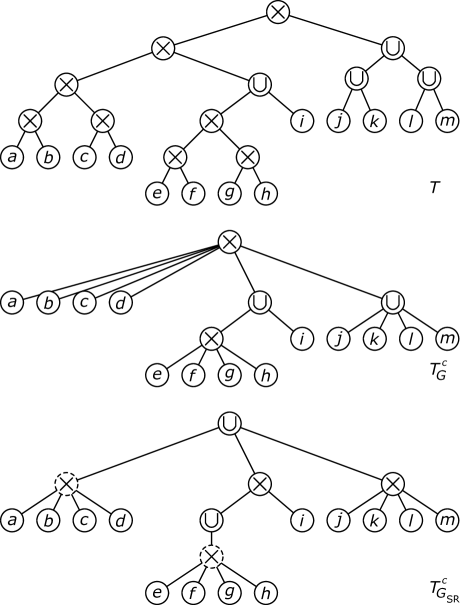
Figure 9: A co-tree $T$ for a co-graph $G$, a canonical co-tree $T^{\text{c}}_{G}$ for $G$, and a canonical co-tree for $T^{\text{c}}_{{G}_{\rm SR}}$ for ${G}_{\rm SR}$. The two nodes with the dashed circles are twin-join nodes in $T^{\text{c}}_{{G}_{\rm SR}}$. These nodes are not in $T^{c}_{G}$.

The size of a minimum strong resolving set for a co-graph $G$ can be computed in linear time by computing the size of a minimum vertex cover for co-graph ${G}_{\rm SR}$. We use the following notations to describe this well-known computation procedure. Let $T$ be a co-tree for a co-graph $G$ with root $\hat{r}$. For a node $\hat{u}$ of $T$, let $T(\hat{u})$ be the subtree of $T$ with root $\hat{u}$ and $\text{n}(\hat{u})$ be the number of leafs in $T(\hat{u})$.

The size of a minimum vertex cover for a co-graph ${G}_{\rm SR}$ with canonical co-tree $T^{c}_{{G}_{\rm SR}}$ and root $\hat{r}$ can be computed in linear time by the bottom-up processing of $T$ with Algorithm 1. The result is $\text{vc}(\hat{r})$, see also Figure 10.

Algorithm 1  $(T^{c}_{{G}_{\rm SR}})$

       for $($each node $\hat{u}$ of $T^{c}_{{G}_{\rm SR}})$ do

             // $-1$ means undefined

             $\text{vc}(\hat{u})\leftarrow-1$;

       end for

      for $($each leaf $\hat{u}$ of $T^{c}_{{G}_{\rm SR}})$ do

             $\text{vc}(\hat{u})\leftarrow 0$;

       end for

      while  $\left(\begin{array}[]{l}\text{there is a node }\hat{u}\text{ of }T^{c}_{{G}_{\rm SR}}\text{ with successor nodes }\hat{u}_{1},\ldots,\hat{u}_{k}\\ \text{such that }\text{\rm vc}({\hat{u}})=-1\text{ and }\text{\rm vc}({\hat{u}_{i}})\geq 0,1\leq i\leq k\end{array}\right)$ do

              

             if $(\hat{u}$ is a union node in $T^{c}_{{G}_{\rm SR}})$ then

                   $\text{vc}({\hat{u}})\leftarrow\text{vc}(\hat{u}_{1})+\cdots+\text{vc}(\hat{u}_{k})$;

             end if

            else

                   // $\hat{u}$ is a join node in $T^{c}_{{G}_{\rm SR}}$

                   $\text{vc}({\hat{u}})\leftarrow\displaystyle\min_{1\leq i\leq k}(\text{n}(\hat{u})-\text{n}(\hat{u}_{i})+\text{vc}(\hat{u}_{i}))$;

                  

             end if

            

       end while

      

Figure 10: The computation of a minimum vertex cover for co-graph ${G}_{\rm SR}$ defined by the canonical co-tree $T^{c}_{{G}_{\rm SR}}$ of Figure 9. The nodes $\hat{u}$ of tree $T^{c}_{{G}_{\rm SR}}$ are labeled $\text{n}(\hat{u})/\text{vc}(\hat{u})$.

However, we need to compute the size of a minimum vertex set that is a vertex cover for ${G}_{\rm SR}$ which contains all vertices that are maximally distant from a vertex $u$ in $G$.

The vertices $v$ that are maximally distant from a vertex $u$ in co-graph $G$ can be specified as follows. Let $T^{c}_{G}$ be a canonical co-tree for $G$ and $\hat{w}$ be the first common ancestor of $\hat{u}={\rm node}(u)$ and $\hat{v}={\rm node}(v)$ in $T^{c}_{G}$.

1. If $\hat{w}$ is a union node, then $u$ and $v$ are not adjacent in $G$ and thus $v$ is maximally distant from $u$ (and $u$ is maximally distant from $v$). Note that connected co-graphs have diameter at most 2.

2. If $\hat{w}$ is a join node, then $u$ and $v$ are adjacent in $G$ and $v$ is maximally distant from $u$ if and only if $N_{G}[v]\subseteq N_{G}[u]$. This is the case if and only if all nodes on the path between $\hat{u}$ and $\hat{w}$ in $T$ are join nodes. If $T^{c}_{G}$ is a canonical co-tree, then this is the case if and only if $\hat{u}$ is a successor node of $\hat{w}$.

For a node $\hat{u}$ of $T^{c}_{G}$ let

$$V(\hat{u})=\{{\rm vertex}(\hat{v})\,|\,\hat{v}\text{ is a leaf of }T^{c}_{G}(\hat{u})\}.$$

A vertex $v$ of $G$ which is not in $V(\hat{u})$ is either adjacent to all vertices of $V(\hat{u})$ or to none of them. This depends on whether the first common predecessor of $\hat{u}$ and ${\rm node}(v)$ in $T$ is a join node or a union node, respectively.

The following algorithm computes a minimum vertex set that is a vertex cover for ${G}_{\rm SR}$ which contains all vertices that are maximally distant from a vertex $w$ in $G$. We assume that $\text{vc}(\hat{u})$ is already computed for each node $\hat{u}$ of $T^{c}_{{G}_{\rm SR}}$ by Algorithm 1.

Algorithm 2  $(T^{c}_{G},T^{c}_{{G}_{\rm SR}},w)$

       $\hat{w}\leftarrow{\rm node}(w)$;

       if $(\hat{w}=\hat{r})$ then

             return 0;

       end if

      Let $\hat{v}$ be the predecessor node of $\hat{w}$ in $T^{c}_{G}$;

       $\text{h}(\hat{v})\leftarrow\text{n}({\hat{v})}-1$;

       while $(\hat{v}\not=\hat{r})$ do

             Let $\hat{u}\leftarrow\hat{v}$;

             Let $\hat{v}$ be the predecessor node of $\hat{u}$ in $T^{c}_{{G}_{\rm SR}}$;

             Let $\hat{u}_{1},\ldots,\hat{u}_{k}$ be the successor nodes of $\hat{v}$ in $T^{c}_{{G}_{\rm SR}}$ without node $\hat{u}$;

             if $(\hat{v}$ is a join node in $T^{c}_{{G}_{\rm SR}})$ then

                   // $\hat{v}$ is a union node in $T^{c}_{G}$

                   $\text{h}(\hat{v})\leftarrow\text{h}(\hat{u})+\text{n}({\hat{u}_{1}})+\cdots+\text{n}({\hat{u}_{k}})$;

             end if

            else

                   // $\hat{v}$ is a union node in $T^{c}_{{G}_{\rm SR}}$

                   // $\hat{v}$ is a join node in $T^{c}_{G}$

                   $\text{h}(\hat{v})\leftarrow\text{h}(\hat{u})+\text{vc}({\hat{u}_{1}})+\cdots+\text{vc}({\hat{u}_{k}})$;

             end if

            

       end while

      return $\text{h}(\hat{r})$;

Algorithm 2 initially sets variable $\text{h}(\hat{v})$ to $\text{n}({\hat{v})}-1$ for the predecessor node $\hat{v}$ of $\hat{w}={\rm node}(w)$ in $T^{c}_{G}$. To explain the correctness of this instruction, we distinguish between the 4 cases shown in Figure 11. In the cases (a), (b), and (c) node $\hat{v}$ is the predecessor node of $\hat{w}$ in $T^{c}_{G}$. In these cases, all vertices of $V(\hat{v})\setminus w$ are maximally distant from $w$ in $G$, based on the second consideration above. One vertex is subtracted here, since vertex $w$ is not maximally distant from $w$ itself if $G$ is connected and has at least two vertices. In case (d), node $\hat{v}$ is a union node in $T^{c}_{G}$ and thus all vertices of $V(\hat{v})\setminus w$ are maximal distant from $w$ based on the first consideration above. If $\hat{v}$ is a node further up on the path to the root $\hat{r}$, we only have to distinguish whether $\hat{v}$ is a join or a union node in $T^{c}_{{G}_{\rm SR}}$. If $\hat{v}$ is a join node in $T^{c}_{{G}_{\rm SR}}$, then $\hat{v}$ is a union node in $T^{c}_{G}$ and all vertices of $V(\hat{v})\setminus V(\hat{u})$ are maximally distant from $w$. If $\hat{v}$ is a union node in $T^{c}_{{G}_{\rm SR}}$, then the minimum vertex covers of the subgraphs induced by the vertex sets $V(\hat{u_{i}})$ of the successor nodes $\hat{u_{i}}$ of $\hat{v}$ without node $\hat{u}$ have to be merged. In this case, node $\hat{v}$ is a join node in $T^{c}_{G}$ and the vertices of $V(\hat{v})\setminus V(\hat{u})$ are not maximal distant from $w$.

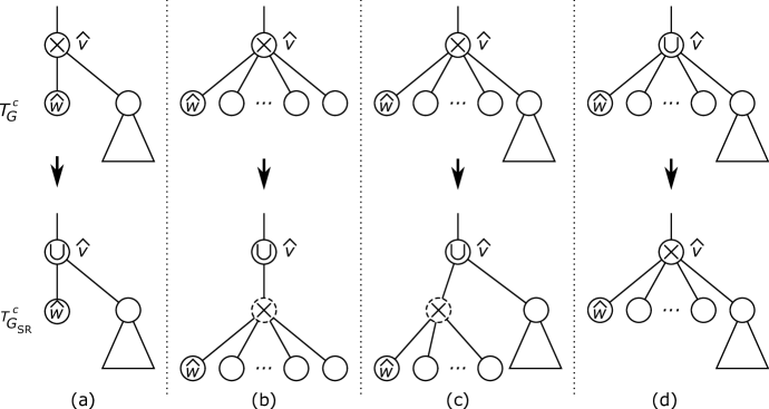
Figure 11: The 4 cases when node $\hat{v}$ is the predecessor node of $\hat{w}$ in $T^{c}_{G}$.

As in Section Section 0.7.2, let

$$h_{i}=|{\overline{\text{VC}}(\,{G(\hat{u})}_{\rm SR}\setminus\{{\rm s}(\hat{v}_{1}),\ldots,{\rm s}(\hat{v}_{k}),{\rm s}(\hat{w})\},\,{\text{MD}(\,G(\hat{u}),\,{\rm s}(\hat{v}_{i})\,)}\setminus\{{\rm s}(\hat{v}_{1}),\ldots,{\rm s}(\hat{v}_{k}),{\rm s}(\hat{w})\}\,)}|$$

and $i_{min}$ be the index $i$ from $\{1,\ldots,k\}$ such that

$$h_{i}\,-\,|{\overline{\text{VC}}(\,{\widetilde{G}(\hat{u_{i}})}_{\rm SR}\setminus\{{\rm s}(\hat{v}_{i})\},\,{\text{MD}(\,\widetilde{G}(\hat{u_{i}}),\,{\rm s}(\hat{v}_{i})\,)}\,)}|$$

is minimal. To determine $i_{\min}$, we have to compute $h_{i}$ for all $i$ in total linear time. To achieve this, we calculate the increments of the values $\text{h}(\hat{u})$ at the inner nodes $\hat{u}$ of $T^{c}_{G}$ along the path to the root $\hat{r}$ top-down in a preprocessing phase. Algorithm 3 computes all these increments, denoted by $\text{m}(\hat{u})$, in total linear time, see also Figure 12.

Algorithm 3  $(T^{c}_{G},T^{c}_{{G}_{\rm SR}})$

       for $($each inner node $\hat{u}$ of $T^{c}_{G})$ do

             // $-1$ means undefined

             $\text{m}(\hat{u})\leftarrow-1$;

       end for

      $\text{m}(\hat{r})\leftarrow 0$;

       while  $\left(\begin{array}[]{l}\text{there is an inner node }\hat{u}\text{ in }T^{c}_{G}\text{ with predecessor node }\hat{v}\\ \text{such that }\text{\rm vc}({\hat{u}})=-1\text{ and }\text{\rm vc}({\hat{v}})\geq 0\end{array}\right)$ do

              

             Let $\hat{u}_{1},\ldots,\hat{u}_{k}$ be the successor nodes of $\hat{v}$ in $T^{c}_{{G}_{\rm SR}}$ without node $\hat{u}$;

             if $(\hat{v}$ is a join node in $T^{c}_{{G}_{\rm SR}})$ then

                   // $\hat{v}$ is a union node in $T^{c}_{G}$

                   $\text{m}(\hat{u})\leftarrow\text{m}(\hat{v})+\text{n}({\hat{u}_{1}})+\cdots+\text{n}({\hat{u}_{k}})$;

             end if

            else

                   // $\hat{v}$ is a union node in $T^{c}_{{G}_{\rm SR}}$

                   // $\hat{v}$ is a join node in $T^{c}_{G}$

                   $\text{m}(\hat{u})\leftarrow\text{m}(\hat{v})+\text{vc}({\hat{u}_{1}})+\cdots+\text{vc}({\hat{u}_{k}})$;

             end if

            

       end while

      

After the pre-processing by Algorithm 3, the size $h_{i}$ of

$${\overline{\text{VC}}(\,{G}_{\rm SR}(\hat{u})),\,{\text{MD}(\,G(\hat{u_{i}}),\,{\rm s}(\hat{v}_{i})\,)}\,)},\,1\leq i\leq k,$$

is computable in time $\mathcal{O}(1)$ as follows. If $\hat{u}$ is the predecessor node of $\hat{u}_{i}$ in $T^{c}_{\widetilde{G}}$, then $h_{i}=\text{n}({\hat{u})}-1+\text{m}(\hat{u})$, see Figure 12.

Figure 12: A canonical co-tree $T^{c}_{{G}_{\rm SR}}$ for a co-graph ${G}_{\rm SR}$. The inner nodes $\hat{u}$ which also exist in $T^{c}_{G}$ are labelled $\text{n}(\hat{u})/\text{vc}(\hat{u})/\text{m}(\hat{u})$ by Algorithm 3. The leafs and the twin-join nodes are labelled only by $\text{n}(\hat{u})/\text{vc}(\hat{u})$. For example,
$\begin{array}[]{lllll}{\overline{\text{VC}}(\,{G}_{\rm SR},\,{\text{MD}(\,G,\,\textsf{{a}}\,)}\,)}&=&13-1+0&=&12,\\ {\overline{\text{VC}}(\,{G}_{\rm SR},\,{\text{MD}(\,G,\,\textsf{{e}}\,)}\,)}&=&4-1+7&=&10,\text{ and}\\ {\overline{\text{VC}}(\,{G}_{\rm SR},\,{\text{MD}(\,G,\,\textsf{{i}}\,)}\,)}&=&5-1+6&=&10.\\ \end{array}$

Finally, we need the size of the set

$$h_{i}=|{\overline{\text{VC}}(\,{G(\hat{u})}_{\rm SR}\setminus\{{\rm s}(\hat{v}_{1}),\ldots,{\rm s}(\hat{v}_{k}),{\rm s}(\hat{w})\},\,{\text{MD}(\,G(\hat{u}),\,x_{i}\,)}\setminus\{{\rm s}(\hat{v}_{1}),\ldots,{\rm s}(\hat{v}_{k}),{\rm s}(\hat{w})\}\,)}|$$

where the nodes ${\rm s}(\hat{v}_{1}),\ldots,{\rm s}(\hat{v}_{k}),{\rm s}(\hat{w})$ are left out from ${G(\hat{u})}_{\rm SR}$. This can be achieved by initially setting the n-values of these nodes to zero and not to 1, see Figure 13. Here, two cases must be distinguished for the calculation of $h_{i}$. If vertex $u$ does not belong to the set of vertices that are excluded, then the calculation of $h_{i}$ is as before $h_{i}=\text{n}(\hat{u})-1+\text{m}(\hat{u})$. However, if node $u$ has been excluded, the computation of $h_{i}$ is $h_{i}=\text{n}(\hat{u})+\text{m}(\hat{u})$. Both cases can be covered by

$$h_{i}=\text{n}(\hat{u})-\text{n}(\hat{w})+\text{m}(\hat{u}).$$

Since index $i_{\min}$ is computable in linear time, the sizes of

• ${\text{VC}(\,{\widetilde{G}(\hat{u})}_{\rm SR}\,)}$,

• ${\text{VC}(\,{\widetilde{G}(\hat{u})}_{\rm SR}\setminus\{{\rm s}(\hat{w})\}\,)}$, and

• ${\overline{\text{VC}}(\,{\widetilde{G}(\hat{u})}_{\rm SR}\setminus\{{\rm s}(\hat{w})\},\,{\text{MD}(\,\widetilde{G}(\hat{u}),\,{\rm s}(\hat{w})\,)}\,)}$

are computable in linear time by Lemmas 7, 8 and 9.

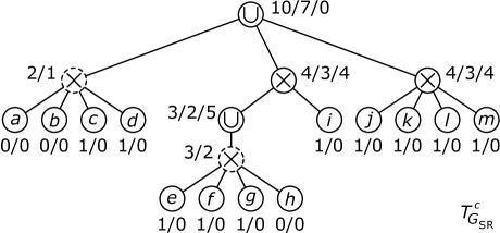
Figure 13: A canonical co-tree $T^{c}_{{G}_{\rm SR}}$ for a co-graph ${G}_{\rm SR}$. The inner nodes $\hat{u}$ which also exist in $T^{c}_{G}$ are labelled $\text{n}(\hat{u})/\text{vc}(\hat{u})/\text{m}(\hat{u})$ by Algorithm 4. The leafs and the twin-join nodes are labelled only by $\text{n}(\hat{u})/\text{vc}(\hat{u})$. Here, the vertices a, b, and h are left out by setting $\text{n}(\textsf{{a}})$, $\text{n}(\textsf{{b}})$, and $\text{n}(\textsf{{h}})$ to zero. For example,
$\begin{array}[]{lllll}{\overline{\text{VC}}(\,{G}_{\rm SR}\setminus\{\textsf{{a}},\textsf{{b}},\textsf{{h}}\},\,{\text{MD}(\,G,\,\textsf{{a}}\,)}\setminus\{\textsf{{a}},\textsf{{b}},\textsf{{h}}\}\,)}&=&10-0+0&=&10,\\ {\overline{\text{VC}}(\,{G}_{\rm SR}\setminus\{\textsf{{a}},\textsf{{b}},\textsf{{h}}\},\,{\text{MD}(\,G,\,\textsf{{e}}\,)}\setminus\{\textsf{{a}},\textsf{{b}},\textsf{{h}}\}\,)}&=&3-1+5&=&7,\text{ and}\\ {\overline{\text{VC}}(\,{G}_{\rm SR}\setminus\{\textsf{{a}},\textsf{{b}},\textsf{{h}}\},\,{\text{MD}(\,G,\,\textsf{{h}}\,)}\setminus\{\textsf{{a}},\textsf{{b}},\textsf{{h}}\}\,)}&=&3-0+5&=&8.\\ \end{array}$

Theorem 5.

A minimum strong resolving set for a graph $G=(V,E)$, in that each biconnected component is a co-graph, can be computed in time ${\mathcal{O}}(|V|+|E|)$.

Ollermann and Peters-Fransen showed in [OP07] that the size of a strong resolving set can be computed in polynomial time for distance hereditary graphs. Graphs in which the biconnected components are co-graphs are distance hereditary, but our solution presented here runs in linear time.

0.8 Conclusion

In this paper we have shown that the efficient computation of a strong resolving set for a graph $G$ essentially depends on the efficient computation of strong resolving sets for its biconnected components. If a minimum strong resolving set can be computed for a biconnected graph in polynomial time, it is generally also possible to compute minimum strong resolving sets in polynomial time, which additionally contain the vertices that are maximally distant from other vertices.

We have given three examples for which it is possible to compute the required assumptions in linear time. From this it could be concluded that the computation of minimum strong resolving sets for graphs is possible in linear time if the biconnected components are circles or co-graphs. It would be interesting to know for which other more complex graph classes this concept is applicable.

A generalization of the procedure for directed graphs and directed strong resolving sets, see for example [SW21], as well as a generalization of the composition of two graphs over several vertices that are all connected to each other are also interesting challenges.

References

- [1]
- [CEJO00] Chartrand, G. ; Eroh, L. ; Johnson, M.A. ; Oellermann, O.: Resolvability in graphs and the metric dimension of a graph. In: Discrete Applied Mathematics 105 (2000), Nr. 1-3, S. 99–113
- [CLB81] Corneil, Derek G. ; Lerchs, Helmut ; Burlingham, L S.: Complement reducible graphs. In: Discrete Applied Mathematics 3 (1981), Nr. 3, S. 163–174
- [DPSL17] Díaz, Josep ; Pottonen, Olli ; Serna, Maria J. ; Leeuwen, Erik J.: Complexity of metric dimension on planar graphs. In: J. Comput. Syst. Sci. 83 (2017), Nr. 1, 132–158. http://dx.doi.org/10.1016/j.jcss.2016.06.006. – DOI 10.1016/j.jcss.2016.06.006
- [FHH+15] Fernau, Henning ; Heggernes, Pinar ; Hof, Pim van’t ; Meister, Daniel ; Saei, Reza: Computing the metric dimension for chain graphs. In: Information Processing Letters 115 (2015), Nr. 9, S. 671–676
- [FM19] Farooq, Rashid ; Mehreen, Naila: Strong metric dimension of generalized Jahangir graph. 2019
- [GJ79] Garey, M.R. ; Johnson, D.S.: Computers and Intractability: A Guide to the Theory of NP-Completeness. W.H. Freeman, 1979. – ISBN 0–7167–1044–7
- [HEW16] Hoffmann, Stefan ; Elterman, Alina ; Wanke, Egon: A linear time algorithm for metric dimension of cactus block graphs. In: Theoretical Computer Science 630 (2016), S. 43–62
- [HM76] Harary, Frank ; Melter, Robert A.: On the metric dimension of a graph. In: Ars Combinatoria 2 (1976), S. 191–195
- [HMP+05] Hernando, M.C. ; Mora, M. ; Pelayo, I.M. ; Seara, C. ; Cáceres, J. ; Puertas, M.L.: On the metric dimension of some families of graphs. In: Electronic Notes in Discrete Mathematics 22 (2005), S. 129–133
- [HP05] Habib, Michel ; Paul, Christophe: A simple linear time algorithm for cograph recognition. In: Discrete Applied Mathematics 145 (2005), Nr. 2, S. 183–197
- [HW12] Hoffmann, S. ; Wanke, E.: Metric Dimension for Gabriel Unit Disk Graphs Is NP-Complete. In: Bar-Noy, Amotz (Hrsg.) ; Halldórsson, Magnús M. (Hrsg.): ALGOSENSORS Bd. 7718, Springer, 2012 (Lecture Notes in Computer Science). – ISBN 978–3–642–36091–6, 90–92
- [IBSS10] Iswadi, H. ; Baskoro, E. ; Salman, A.N.M. ; Simanjuntak, R.: The metric dimension of amalgamation of cycles. In: Far East Journal of Mathematical Sciences (FJMS) 41 (2010), Nr. 1, S. 19–31
- [JO95] Jamison, Beverly ; Olariu, Stephan: A Linear-Time Recognition Algorithm for P4-Reducible Graphs. In: Theor. Comput. Sci. 145 (1995), Nr. 1&2, 329–344. http://dx.doi.org/10.1016/0304-3975(95)00016-P. – DOI 10.1016/0304–3975(95)00016–P
- [KRR96] Khuller, Samir ; Raghavachari, Balaji ; Rosenfeld, Azriel: Landmarks in Graphs. In: Discrete Applied Mathematics 70 (1996), S. 217–229
- [Kuz20] Kuziak, Dorota: The Strong Resolving Graph and the Strong Metric Dimension of Cactus Graphs. In: Mathematics 8 (2020), Aug, Nr. 8, S. 1266. http://dx.doi.org/http://doi.org/10.3390/math8081266. – DOI http://doi.org/10.3390/math8081266. – ISSN 2227–7390
- [KYR13] Kuziak, Dorota ; Yero, Ismael G. ; Rodríguez-Velázquez, Juan A.: On the strong metric dimension of corona product graphs and join graphs. In: Discrete Applied Mathematics 161 (2013), Nr. 7-8, 1022–1027. http://dx.doi.org/10.1016/j.dam.2012.10.009. – DOI 10.1016/j.dam.2012.10.009
- [KYRV16] Kuziak, Dorota ; Yero, Ismael G. ; Rodríguez-Velázquez, Juan A.: Strong metric dimension of rooted product graphs. In: International Journal of Computer Mathematics 93 (2016), Nr. 8, S. 1265–1280. http://dx.doi.org/10.1080/00207160.2015.1061656. – DOI 10.1080/00207160.2015.1061656
- [LZZ20] Liu, Jia-Bao ; Zafari, Ali ; Zarei, Hassan: Metric Dimension, Minimal Doubly Resolving Sets, and the Strong Metric Dimension for Jellyfish Graph and Cocktail Party Graph. In: Complexity 2020 (2020). http://dx.doi.org/https://doi.org/10.1155/2020/9407456. – DOI https://doi.org/10.1155/2020/9407456
- [MRGS15] Manuel, Paul ; Rajan, Bharati ; Grigorious, Cyriac ; Stephen, Sudeep: On the Strong Metric Dimension of Tetrahedral Diamond Lattice. In: Mathematics in Computer Science 9 (2015), Jun, Nr. 2, S. 201–208. http://dx.doi.org/10.1007/s11786-015-0226-0. – DOI 10.1007/s11786–015–0226–0. – ISSN 1661–8289
- [MT84] Melter, R.A. ; Tomescu, I.: Metric bases in digital geometry. In: Computer Vision, Graphics, and Image Processing 25 (1984), Nr. 1, S. 113–121
- [OP07] Oellermann, Ortrud R. ; Peters-Fransen, Joel: The strong metric dimension of graphs and digraphs. In: Discrete Applied Mathematics 155 (2007), Nr. 3, 356–364. http://dx.doi.org/10.1016/j.dam.2006.06.009. – DOI 10.1016/j.dam.2006.06.009
- [RVYKO14] Rodríguez-Velázquez, Juan A. ; Yero, Ismael G. ; Kuziak, Dorota ; Oellermann, Ortrud R.: On the strong metric dimension of Cartesian and direct products of graphs. In: Discrete Mathematics 335 (2014), 8 - 19. http://dx.doi.org/https://doi.org/10.1016/j.disc.2014.06.023. – DOI https://doi.org/10.1016/j.disc.2014.06.023. – ISSN 0012–365X
- [SBS+11] Saputro, S.W. ; Baskoro, E.T. ; Salman, A.N.M. ; Suprijanto, D. ; Baca, A.M.: The Metric Dimension of Regular Bipartite Graphs. In: arXiv/1101.3624 (2011). http://arxiv.org/abs/1101.3624
- [Sla75] Slater, Peter J.: Leaves of trees. In: Congressum Numerantium 14 (1975), S. 549–559
- [Sla88] Slater, Peter J.: Dominating and reference sets in a graph. In: Journal of Mathematical and Physical Sciences 22 (1988), S. 445 – 455
- [ST04] Sebö, András ; Tannier, Eric: On Metric Generators of Graphs. In: Mathematics of Operations Research 29 (2004), Nr. 2, 383–393. http://dx.doi.org/10.1287/moor.1030.0070. – DOI 10.1287/moor.1030.0070
- [SW21] Schmitz, Yannick ; Wanke, Egon: On the Strong Metric Dimension of directed co-graphs. In: CoRR abs/2111.13054 (2021). https://arxiv.org/abs/2111.13054
- [VHW19] Vietz, Duygu ; Hoffmann, Stefan ; Wanke, Egon: Computing the Metric Dimension by Decomposing Graphs into Extended Biconnected Components - (Extended Abstract). In: Das, Gautam K. (Hrsg.) ; Mandal, Partha S. (Hrsg.) ; Mukhopadhyaya, Krishnendu (Hrsg.) ; Nakano, Shin-Ichi (Hrsg.): WALCOM: Algorithms and Computation - 13th International Conference, WALCOM 2019, Guwahati, India, February 27 - March 2, 2019, Proceedings Bd. 11355, Springer, 2019 (Lecture Notes in Computer Science), 175–187
- [WK18] Widyaningrum, Mila ; Kusmayadi, Tri A.: On the strong metric dimension of sun graph, windmill graph, and möbius ladder graph. In: Journal of Physics: Conference Series 1008 (2018), apr, 12-32. http://dx.doi.org/10.1088/1742-6596/1008/1/012032. – DOI 10.1088/1742–6596/1008/1/012032