Two-dimensional regular string black hole
via complete corrections
Shuxuan Ying
ysxuan@cqu.edu.cnDepartment of Physics, Chongqing University, Chongqing, 401331, China
Abstract
In string theory, an important challenge is to show if the singularity of black holes can be smoothed out by the complete corrections. The simplest case is to consider a 2D string black hole or 3D black string. This problem was discussed in a gauged Wess-Zumino-Witten (WZW) model and the results are supposed to be correct to all orders in corrections. Based on the recent remarkable progress on classifying all the corrections, in this work, we re-study this problem with the low energy effective spacetime action, and provide classes of exact non-perturbative and non-singular solutions of the 2D black hole/3D black string via complete corrections.
††preprint: APS/123-QED
How to resolve a singularity of a black hole is a long-standing problem
in general relativity. It is well-known that the black hole possesses
two kinds of infinities: one is the coordinate singularity which can be removed by
coordinates transformations;
another is the curvature singularity which cannot be smoothed out and is unavoidable in Einstein’s
gravity Penrose:1964wq ; Hawking:1965mf . The regular black hole
solutions must satisfy two requirements: I) The curvature invariants
(such as Kretschmann scalar) are regular everywhere; II) The geodesics
are complete. However, there is yet
no systematic methods to obtain regular solutions from solving
Einstein’s equation exactly without any ad hoc settings. People
therefore expect a theory of quantum gravity will provide inspirations
to solve this problem completely. String theory as one candidate of
quantum gravitational theories should be able to answer this question.
The simplest black hole solution in string theory, namely 1+1 dimensional
string black hole, was obtained by solving a 2D closed string’s low
energy effective action Mandal:1991tz ; Lemos:1993py . This solution is only
valid when the string length scale is small
compared to the radius of spacetime curvature. One may wonder how
to obtain the exact string black hole solutions of the full action,
and whether the spacetime singularity disappears in these solutions.
However, it looks impossible since the low energy effective action
with complete corrections is unknown. As an alternative,
Witten obtained the exact metric which described the region outside
the event horizon of 2D string black hole through the
gauged WZW model, this result is conformally invariant to all orders
in when ( is
the Kac–Moody level) Witten:1991 . This metric still possesses
a curvature singularity in the maximally extended
spacetime. Then, in ref. Dijkgraaf:1991ba , Dijkgraaf, Verlinde
and Verlinde discovered the exact 2D string black hole for general
, which was supposed to be correct to all orders in .
Based on this work, Perry and Teo Perry:1993ry , and Yi Yi:1993gh
studied its maximally extended spacetime. The Weyl invariance
of this solution is then verified by Tseytlin up to 3-loops ()
in the bosonic sigma modelTseytlin:1991ht .
The supersymmetric 4-loops () was also checked in
ref. Jack:1992mk .
In recent works Hohm:2015doa ; Hohm:2019ccp ; Hohm:2019jgu , Hohm
and Zwiebach reconsidered how to classify all orders
corrections of the low energy effective action. This progress makes
it possible to re-study the exact 2D string black hole systematically.
Hohm and Zwiebach’s motivation was based on two reasons: I) the tree-level
string effective action and its first order correction
can be put into an explicit covariant form by
suitable field redefinitions Veneziano:1991ek ; Sen:1991zi ; Sen:1991cn ; Meissner:1991zj ; Meissner:1996sa ;
II) Sen proved that for configurations independent of coordinates,
all orders in expansion possess the
symmetry Sen:1991zi ; Sen:1991cn . Hohm and Zwiebach therefore
assumed that the standard matrix always keep
its form unchanged to all orders in , meanwhile
the -breaking terms could be absorbed into the
standard matrix by the field redefinitions. With this assumption,
Hohm and Zwiebach showed that all orders in are
classified by even powers of Hubble parameter in FLRW cosmological
background. The dilaton appears trivially and only first order time
derivatives need to be included. Since the equations of motion (EOM)
only include first two derivatives of spacetime metric, the theory
is ghost free and exactly solvable. This significant progress makes
it possible to study non-perturbative stringy effects. Based on this
work, we have found that the big-bang singularity could be smoothed
out by the complete corrections Wang:2019kez ; Wang:2019dcj .
It is also proved that the Hohm and Zwiebach’s derivation can also
apply to the domain wall background Wang:2019mwi , so that
the naked singularities can be resolved Ying:2021xse . Based on these attempts,
it is reasonable to believe that the corrections will resolve the singularity
of black hole Bars:1992sr . However, the process is
tricky for the general spherically symmetric black holes, because they break the
symmetry and Hohm-Zwiebach action cannot be derived from this background.
As an alternative, we consider the 2D black hole/3D black string at first.
In this paper, our aim is to find regular solutions which exactly
solve the EOM of completely corrected closed string
theory. In the perturbative region
, it reduces to traditional 2D black
hole/3D black string. At first, let us start by the 2D low energy effective action
of closed string:
(1)
where is the string metric, is the
physical dilaton,
and we set Kalb-Ramond field for simplicity.
This two dimensional gravity has dynamics due to a pre-factor .
The black hole solution of this action is given by Mandal:1991tz :
(2)
where we set an integral constant in
for simplicity. If we add a direction in this metric,
it is called a black string solution and firstly discovered by Horne
and Horowitz Horne:1991gn . The difference betwween 2D and 3D theories is only due to its definition. When we consider the extra dimension , the 3D black string solution is a simple product of and the two dimensional metric, which does not affect the action Horne:1991gn . Therefore, although we only study the 2D black
hole in this paper, our result also applies to the 3D black string. Back to the metric (2)
, the event horizon is located at and its curvature singularity
is due to a scalar curvature . Keep in mind that there are two kinds of
coordinate transformations which cover different regions of maximally
extended spacetime. The first one is
(3)
where and . Utilizing this coordinate
transformation, the metric (2) becomes
(4)
where invariant dilaton is defined by
(5)
This metric is well-known as Witten’s 2D black hole solution,
which was obtained by the gauged
WZW model Witten:1991 . This metric could be applied in Hohm-Zwiebach
action directly. However, it does not possess a curvature singularity
since it only describes the region outside the event horizon
(), and the scalar curvature
is regular in this region. To discover the curvature singularity
of the metric (2), we need to adopt
the second kind of coordinate transformations:
(6)
where and we only consider one period,
namely . Based on this transformation,
the metric (2) becomes
(7)
which describes the inner metric of black hole, and
here plays a role as the time-like direction.This metric (7)
topologically corresponds to an annulus. The event horizon is located at
and the curvature singularity is the boundary
due to the scalar curvature .
Our aim is to remove the curvature singularity of (7)
by the complete corrections.
The closed string fields which depend on this metric possess
symmetry. It is worth noting that we can also use the ansatz (2), which shares the same result with (7) by the coordinate transformation (6).
Based on this ansatz, Hohm and Zwiebach
showed that the following low energy effective action with complete
corrections could be rewritten as
where ,
,
, , ,
and ’s
are unknown coefficients for a bosonic case Codina:2021cxh .
In addition, the symmetry of the action (LABEL:eq:Odd_action_with_alpha)
is manifested by the following transformations:
(10)
To match the model (1),
we need to add an invariant constant
into the action (LABEL:eq:Odd_action_with_alpha):
(11)
which is also a scalar under the general coordinate transformations.
The EOM then is
(12)
where
(13)
and there is an extra constraint .
It is easy to check that the solution (4) and
(7) satisfy the EOM (12)
at zeroth order in . Furthermore, we wish to stress
that is any positive real number in the EOM (12)
and the action (LABEL:eq:Odd_action_with_alpha). Therefore, eq. (13)
are not the simple expansions in the limit ,
but the non-perturbative series in general .
To remove the curvature singularity of \textcolorred(7) to
obtain a non-perturbative and non-singular solution of EOM (12)
with complete corrections, there are two requirements:
•
The solutions are assumed to be regular everywhere for general
.
•
In the perturbative regime, namely, as ,
the solutions must reduce to the perturbative solutions of EOM (12).
Although, we know that 6
when which satisfies the condition ,
we treat as a general value here as in
Dijkgraaf:1991ba .
In the body, we present one class of general non-perturbative solution
which covers all coefficients . In the Appendix A, we will give
other possible general solutions. Now, let us start by calculating
the perturbative solutions of EOM (12). For convenience,
we introduce a new variable as
Based on the perturbative solutions (18)
and (19) up to any higher order,
we can figure out the general non-perturbative and non-singular solution
which exactly solves the EOM (12) and covers
all coefficients :
(20)
where ’s are functions of and
. After obtained regular , the regularity of
, and
is guaranteed due to the EOM (12).
Moreover, in the perturbative regime ,
the general solution is expanded as,
(21)
To analyze the general solution (20),
we choose the special case whose perturbative expansion only covers
and . It is not difficult
to check that the general solution (20) which covers the coefficients
does not affect our following argument due to the ref. Wang:2019dcj . Therefore, to match the expansion
(21) with the perturbative solution
(19), we can fix the functions ,
and such that
Based on the ansatz (8), Kretschmann scalar
is given by .
Therefore, the regular solution exists when
in the region . From the solution (LABEL:eq:solution),
we will get
(23)
and physical dilaton,
(24)
where and
are elliptic integrals of the first and second kinds, and is
an integral constant. Now, we set ,
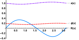
, and plot ,
and in the region
as an example, see Fig. (1).
Figure 1: The figure of ,
and at .
In Fig. (1), it is easy to see
that , and
are regular in the region . To see
how corrections affects the property of the curvature
singularity, we can see the following figure.
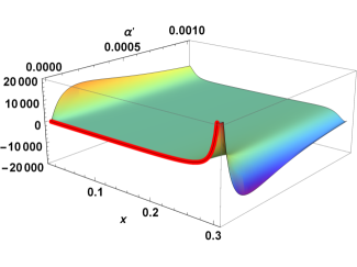
Figure 2: The figure of ,
where ,
and . The
curvature singularity locates at
when .
In Fig. (2), it presents
the behavior of Ricci scalar of the solution (LABEL:eq:solution).
When goes to zero, reduces to
(Red solid line), which possesses the curvature singularity at .
On the other hand, when grows up, the curvature
singularity disappears and becomes regular everywhere.
Finally, we need to stress the relations between the Dijkgraaf et
al.’s exact string black hole Dijkgraaf:1991ba and our result.
As expected, the perturbative solutions (18)
and (19) of Hohm-Zwiebach action
matches with expansion of Dijkgraaf et al.’s solution
up to two-orders. The verification requires to know the higher-loop
-function and Hohm-Zwiebach action simultaneously, and it
is not straightforward since there exits a series of field redefinitions
from the higher-loop -function to the EOM of Hohm-Zwiebach
action. Each field redefinition modifies the EOM and their corresponding
perturbative solutions. In Appendix B, we present the simple example
of field redefinitions up to the first-order correction.
Beyond second-order correction, the -functions
are unknown. It is therefore impossible to verify the correctness
of the Dijkgraaf et al.’s solution to all orders in
through the Hohm-Zwiebach action.
In short, we used the complete corrections of closed
string theory to remove the singularity of 2D black hole or 3D black
string. We looked for the
regular black hole solution (LABEL:eq:solution) which exactly solves
the EOM of Hohm-Zwiebach action. In the perturbative limit ,
Witten’s 2D black hole solution is recovered. The T-dual solutions can be achieved by simply replacing
in eq. (23). Moreover, it is worthwhile to study how to obtain other exact solution (which possesses two spacetime sigularities) of coset model Sfetsos:1992yi from the Hohm-Zwiebach action.
Acknowledgements.
We thank the useful discussions with Xin Li, Peng Wang, Houwen Wu,
Haitang Yang. This work is supported by the NSFC Grant No. 12105031.
References
(1)
R. Penrose, “Gravitational collapse and space-time singularities,” Phys. Rev. Lett. 14, 57-59 (1965) doi:10.1103/PhysRevLett.14.57
(2)
S. Hawking, “Occurrence of singularities in open universes,” Phys. Rev. Lett. 15, 689-690 (1965) doi:10.1103/PhysRevLett.15.689
(3)
G. Mandal, A. M. Sengupta and S. R. Wadia, “Classical solutions of two-dimensional string theory,” Mod. Phys. Lett. A 6, 1685-1692 (1991) doi:10.1142/S0217732391001822
(4)
J. P. S. Lemos and P. M. Sa,
“The Black holes of a general two-dimensional dilaton gravity theory,”
Phys. Rev. D 49, 2897-2908 (1994)
[erratum: Phys. Rev. D 51, 5967-5968 (1995)]
doi:10.1103/PhysRevD.49.2897
[arXiv:gr-qc/9311008 [gr-qc]].
(5)
E. Witten, “String theory and black holes,” Phys. Rev. D 44, 314 (1991) doi:10.1103/PhysRevD.44.314
(6)
R. Dijkgraaf, H. L. Verlinde and E. P. Verlinde, “String propagation in a black hole geometry,” Nucl. Phys. B 371, 269-314 (1992) doi:10.1016/0550-3213(92)90237-6
(7) M. J. Perry and E. Teo, “Nonsingularity of the exact two-dimensional string black hole,” Phys. Rev. Lett. 70, 2669-2672 (1993) doi:10.1103/PhysRevLett.70.2669 [arXiv:hep-th/9302037 [hep-th]].
(8) P. Yi, “Nonsingular 2-D black holes and classical string backgrounds,” Phys. Rev. D 48, 2777-2788 (1993) doi:10.1103/PhysRevD.48.2777 [arXiv:hep-th/9302070 [hep-th]].
(9)
I. Bars and K. Sfetsos, “Conformally exact metric and dilaton in string theory on curved space-time,” Phys. Rev. D 46, 4510-4519 (1992) doi:10.1103/PhysRevD.46.4510 [arXiv:hep-th/9206006 [hep-th]].
(10) A. A. Tseytlin, “On the form of the black hole solution in D = 2 theory,” Phys. Lett. B 268, 175-178 (1991) doi:10.1016/0370-2693(91)90800-6
(11)
I. Jack, D. R. T. Jones and J. Panvel, “Exact bosonic and supersymmetric string black hole solutions,” Nucl. Phys. B 393, 95-110 (1993) doi:10.1016/0550-3213(93)90239-L [arXiv:hep-th/9201039 [hep-th]].
(12)
O. Hohm and B. Zwiebach, “T-duality Constraints on Higher Derivatives Revisited,” JHEP 1604, 101 (2016) doi:10.1007/JHEP04(2016)101 [arXiv:1510.00005 [hep-th]].
(13)
O. Hohm and B. Zwiebach, “Non-perturbative de Sitter vacua via corrections,” Int. J. Mod. Phys. D 28, no.14, 1943002 (2019) doi:10.1142/S0218271819430028 [arXiv:1905.06583 [hep-th]].
(14)
O. Hohm and B. Zwiebach, “Duality invariant cosmology to all orders in ’,” Phys. Rev. D 100, no.12, 126011 (2019) doi:10.1103/PhysRevD.100.126011 [arXiv:1905.06963 [hep-th]].
(15)
G. Veneziano, “Scale factor duality for classical and quantum strings,” Phys. Lett. B 265, 287 (1991). doi:10.1016/0370-2693(91)90055-U
(16)
K. A. Meissner and G. Veneziano, “Symmetries of cosmological superstring vacua,” Phys. Lett. B 267, 33 (1991). doi:10.1016/0370-2693(91)90520-Z
(17)
A. Sen, “O(d) x O(d) symmetry of the space of cosmological solutions in string theory, scale factor duality and two-dimensional black holes,” Phys. Lett. B 271, 295 (1991). doi:10.1016/0370-2693(91)90090-D
(18)
A. Sen, “Twisted black p-brane solutions in string theory,” Phys. Lett. B 274, 34 (1992) doi:10.1016/0370-2693(92)90300-S [hep-th/9108011].
(19)
K. A. Meissner, “Symmetries of higher order string gravity actions,” Phys. Lett. B 392, 298 (1997) doi:10.1016/S0370-2693(96)01556-0 [hep-th/9610131].
(20)
P. Wang, H. Wu, H. Yang and S. Ying, “Non-singular string cosmology via corrections,” JHEP 1910, 263 (2019) doi:10.1007/JHEP10(2019)263 [arXiv:1909.00830 [hep-th]].
(21)
P. Wang, H. Wu, H. Yang and S. Ying, “Construct corrected or loop corrected solutions without curvature singularities,” JHEP 01, 164 (2020) doi:10.1007/JHEP01(2020)164 [arXiv:1910.05808 [hep-th]].
(22)
P. Wang, H. Wu and H. Yang, “Are nonperturbative AdS vacua possible in bosonic string theory?,” Phys. Rev. D 100, no. 4, 046016 (2019) doi:10.1103/PhysRevD.100.046016 [arXiv:1906.09650 [hep-th]].
(23)
S. Ying, “Resolving naked singularities in -corrected string theory,”
Eur. Phys. J. C 82, no.6, 523 (2022)
doi:10.1140/epjc/s10052-022-10427-5
[arXiv:2112.03087 [hep-th]].
(24)
J. H. Horne and G. T. Horowitz, “Exact black string solutions in three-dimensions,” Nucl. Phys. B 368, 444-462 (1992) doi:10.1016/0550-3213(92)90536-K [arXiv:hep-th/9108001 [hep-th]].
(25)
T. Codina, O. Hohm and D. Marques, “General string cosmologies at order ’3,”
Phys. Rev. D 104, no.10, 106007 (2021)
doi:10.1103/PhysRevD.104.106007
[arXiv:2107.00053 [hep-th]].
(26)
K. Sfetsos, “Conformally exact results for SL(2,R) x SO(1,1)(d-2) / SO(1,1) coset models,”
Nucl. Phys. B 389, 424-444 (1993)
doi:10.1016/0550-3213(93)90327-L
[arXiv:hep-th/9206048 [hep-th]].
Appendix A
Supposing the coefficients are known, to figure out
the non-perturbative solutions, we can choose a different kind of
ansatz. Here, we present two simple examples. The first possible ansatz
is
(25)
where ’s are functions of and coefficients
. Singularities appear if and only if
(26)
If we wish to cover the first two terms of the perturbative
solution, we set . In the perturbative regime ,
the ansatz in (25) is expanded
as
(27)
To match the perturbative solution, ’s can be
fixed as
(28)
The second ansatz is given by
(29)
where ’s are functions of and
coefficients . Singularities appear if and only if
(30)
In the perturbative regime ,
the ansatz in (29) is expanded
as
(31)
To match the perturbative solution, ’s can
be fixed as
(32)
Appendix B
Considering the FLRW ansatz
(33)
the ordinary low energy effective action with the first-order
correction becomes
(34)
The corresponding perturbative solution is
(35)
which is consistent with Dijkgraaf et al.’s result inside
the event horizon up to the first-order correction.
Using the field redefinitions,
(36)
where
the action becomes Hohm-Zwiebach action with the first-order
correction after setting ,