Generalizing Choi map in $M_{3}$ beyond circulant scenario

Abstract

We present a generalization of the family of linear positive maps in $M_{3}$ proposed thirty years ago by Cho et al. (Linear Algebra Appl. 171, 213 (1992)) as a generalization of the seminal Choi non-decomposable map. The necessary and sufficient conditions for decomposability are provided.

I Introduction

Positive linear maps in matrix algebras play important role both in mathematics and physics Stormer-63 ; Stormer ; Paulsen ; Tomiyama1 ; Tomiyama2 ; Tomiyama3 ; Bhatia ; HHHH ; Guhne ; TOPICAL . Let $M_{n}$ denote a $C^{*}$-algebra of $n\times n$ complex matrices. A linear map $\Phi:M_{n}\to M_{m}$ is positive if $\Phi(X)\geq 0$ for all $X\geq 0$. The structure of a convex cone ${\cal P}_{n,m}$ of positive maps from $M_{n}$ to $M_{m}$ is still not fully understood MM ; OSID ; CMP ; KOREA ; Ha-Kye ; TOPICAL . Due to Woronowicz Woronowicz the cones ${\cal P}_{2,2}$, ${\cal P}_{2,3}$, and ${\cal P}_{3,2}$ consist of decomposable maps only, that is, maps which can be decomposed as follows

$$\Phi=\Phi_{1}+\Phi_{2}\circ{\rm T},$$ (1)

where $\Phi_{1},\Phi_{2}$ are completely positive, and ${\rm T}$ denotes a matrix transposition. Recall that a positive map $\Phi\in{\cal P}_{n,m}$ is completely positive if the extended map

$$\Phi^{(k)}:={\rm id}_{k}\otimes\Phi:M_{k}(M_{n})\to M_{k}(M_{m}),$$ (2)

is positive for all $k=1,2,\ldots$ (${\rm id}_{k}$ denotes an identity map in $M_{k}$). Actually, due to Choi-75 , the map $\Phi$ is complete positive if $\Phi^{(k)}$ is positive for $k={\rm min}\{n,m\}$. A first example of a non-decomposable map in $\mathcal{P}_{3,3}$ was provided by Choi Choi1 ; Choi2 ; Choi3

$$\Phi(X)=\begin{bmatrix}x_{11}+x_{22}&-x_{12}&-x_{13}\\ -x_{21}&x_{22}+x_{33}&-x_{23}\\ -x_{31}&-x_{32}&x_{33}+x_{11}\end{bmatrix},$$ (3)

with $X=\{x_{ij}\}\in M_{3}$. Choi map (3) was then generalized to a 3-parameter family of maps Korea1

$$\Phi_{C}(X)=D(X)-X,$$ (4)

where $D(X)$ is a diagonal matrix with $D_{ii}=\sum_{j=1}^{3}C_{ij}x_{jj}$, and $C=\{C_{ij}\}$ is a $3\times 3$ circulant matrix in the following form

$$C=\begin{bmatrix}a&b&c\\ c&a&b\\ b&c&a\end{bmatrix},\ \ \ a,b,c\geq 0.$$ (5)

For $(a,b,c)=(2,1,0)$ the map (4) reduces to (3). The authors of Korea1 proved the following:

Theorem 1.

The map $\Phi_{C}$ defined in (4) is positive if and only if

• $a\geq 1$,

• $a+b+c\geq 3$,

• if $a\leq 2$, then $bc\geq(2-a)^{2}$.

For $a<3$, the positive map $\Phi_{C}$ is decomposable if and only if

$$bc\geq\left(\frac{3-a}{2}\right)^{2}.$$ (6)

If $a\geq 3$, then $\Phi_{C}$ is completely positive (and hence decomposable).

In this paper, we generalize the above result for a class of maps defined in (4), where now $D(X)$ is a diagonal matrix with $D_{ii}=\sum_{j=1}^{3}w_{ij}x_{jj}$, and $W=\{w_{ij}\}\in M_{3}$ such that $w_{ij}\geq 0$ and

$$\sum_{i=1}^{3}w_{ij}=\sum_{j=1}^{3}w_{ij}=w,$$ (7)

i.e. $W/w=\{w_{ij}/w\}$ is a doubly stochastic matrix. In what follows a map defined in terms of the matrix $W$ by $\Phi_{W}$. It is clear that when $W=[w_{ij}]$ is circulant, then our class reduces to the from (4).

This paper is organized as follows. In Sec. II, we derive the conditions for positivity of the map $\Phi_{W}$. In Sec. III, we present a new parameterization for $W$ from Birkhoff theorem and analyze the obtained family of positive maps. The necessary and sufficient condition for decomposability is discussed in Sec. IV. Finally, in Sec. V, we provide concluding remarks.

II positivity

Let us consider a linear map $\Phi_{W}$ parameterized by a $3\times 3$ matrix $W$ with non-negative entries $\{w_{ij}\}$. Note that $\Phi_{W}$ is completely positive if and only if

$$\left(\begin{array}[]{ccc}w_{11}-1&-1&-1\\ -1&w_{22}-1&-1\\ -1&-1&w_{33}-1\end{array}\right)\geq 0.$$ (8)

The above condition is equivalent to

$$\frac{1}{w_{11}}+\frac{1}{w_{22}}+\frac{1}{w_{33}}\leq 1.$$ (9)

It means that the harmonic mean

$$H({w_{11}},{w_{22}},{w_{33}})\geq 3.$$ (10)

In particular, if all $w_{ii}=a$, then (8) is equivalent to $H(a,a,a)=a\geq 3$. Now we find the conditions upon $W$ which guarantee that $\Phi_{W}$ is positive. It is enough to check the positivity for rank-one positive matrices $X=\psi\psi^{\dagger}$:

$$\forall\psi\in\mathbb{C}^{3},\quad\Phi_{W}(\psi\psi^{\dagger})=\mathrm{diag}\left(\sum_{i=1}^{3}w_{1i}|\psi|^{2}_{i},\sum_{i=1}^{3}w_{2i}|\psi|^{2}_{i},\sum_{i=1}^{3}w_{3i}|\psi|^{2}_{i}\right)-\psi\psi^{\dagger}\geq 0.$$ (11)

Let us denote $x_{i}=|\psi_{i}|^{2}$, $z_{i}=\sum_{j=1}^{3}w_{ij}x_{j}$. The principal minor $M_{I}$ of $\Phi_{W}(\psi\psi^{\dagger})$, constructed from the rows and columns of indices from the set $I\subset\{1,2,3\}$ is equal to

$$M_{I}(\vec{x})=\prod_{i\in I}z_{i}-\sum_{i\in I}x_{i}\prod_{j\in I\setminus\{i\}}z_{j},\qquad\mbox{with }\prod_{j\in\emptyset}z_{j}=1.$$ (12)

Observe that, the positivity depends only on modules of $x_{i}$, and not on their phases. Moreover, the norm of $\psi$, equals to $x_{1}+x_{2}+x_{3}$, is irrelevant for positivity. Hence one can rewrite the condition (11) as:

$$\forall\vec{x}\in\Delta^{2},\leavevmode\nobreak\ \ \forall I\subset\{1,2,3\},\leavevmode\nobreak\ \ M_{I}(\vec{x})\geq 0,$$ (13)

where $\Delta^{2}$ denotes the 2-simplex with vertices $x_{i}$. Observe that, at most one eigenvalue of $\Phi_{W}(\psi\psi^{\dagger})$ can be negative since it is obtained as a semi-positive matrix minus rank-one semi-positive matrix, hence in the generic case it is enough to check its determinant, i.e. $M_{\{1,2,3\}}$. Specifically, when $x_{i}=0$ and the corresponding $z_{i}=0$ might not be straightforward to determine the positivity. Then, the determinant can be zero, but the matrix $\Phi_{W}(\psi\psi^{\dagger})$ can have a negative diagonal block. Therefore when some components of $x_{i}$ are zero and the $\Phi_{W}(\psi\psi^{\dagger})$ obtains the block-diagonal structure, the solution is to analyze the positivity of the maximal non-trivial block.

Proceeding in this way, we will check the above condition on disjoints subsets of $\Delta^{2}$ emerging from its cellular decomposition, i.e. on the interior, on the edges and in the vertices.

In the vertices of $\Delta^{2}$ (where any two components of $x_{i}$’s are zero), the positivity of $M_{\{1,2,3\}}(\vec{x})$ reduces to positivity of size-1 minors and one obtains:

$$w_{ii}\geq 1,\qquad i=1,2,3.$$ (14)

In an edge of $\Delta^{2}$ (where any one component of $x_{i}$ is zero), let’s say for $x_{3}=0$, the positivity of $M_{\{1,2,3\}}(\vec{x})$ reduces to positivity of $M_{\{1,2\}}=z_{1}z_{2}-x_{1}z_{2}-x_{2}z_{1}$:

$$(w_{11}-1)w_{21}x_{1}^{2}+(w_{22}-1)w_{12}x_{2}^{2}+[(w_{11}-1)(w_{22}-1)-1+w_{12}w_{21}]x_{1}x_{2}\geq 0.$$ (15)

Using (14), the above quadratic form is non-negative for positive $x_{1},x_{2}$ iff $((w_{11}-1)(w_{22}-1)-1+w_{12}w_{21})>-2\sqrt{(w_{11}-1)(w_{22}-1)w_{21}w_{12}}$, which can be simplified as

$$\sqrt{(w_{11}-1)(w_{22}-1)}+\sqrt{w_{12}w_{21}}\geq 1.$$ (16)

Similar conditions arise from the remaining edges. Summarizing the edge conditions read

$$\sqrt{(w_{ii}-1)(w_{jj}-1)}+\sqrt{w_{ij}w_{ji}}\geq 1,$$ (17)

for $i\neq j$. Note that, for $i=j$, condition (17) is equivalent to the vertex condition (14).

In the interior of $\Delta^{2}$, denoting as $\mathrm{Int}\Delta^{2}$ (where all $x_{i}>0$), the positivity of $M_{\{1,2,3\}}$ gives the third order polynomial inequality of $x_{1},x_{2},x_{3}$:

$$\forall\vec{x}\in\mathrm{Int}\Delta^{2},\ z_{1}z_{2}z_{3}-x_{1}z_{2}z_{3}-x_{2}z_{3}z_{1}-x_{3}z_{1}z_{2}\geq 0.$$ (18)

We want to find the values of local maxima of the LHS in (18). Substituting $x_{3}=1-x_{2}-x_{1}$ and demanding partial derivatives with respect to $x_{1},x_{2}$ to be zero, one obtains a system of two second order equations, which have in general four solutions for extrema, arising from roots of a four-order polynomial. Hence, in general, the problem of finding the local maxima for ‘$z_{1}z_{2}z_{3}-x_{1}z_{2}z_{3}-x_{2}z_{3}z_{1}-x_{3}z_{1}z_{2}$’ is quite involve. Note that, condition (18) may be equivalently rewritten as follows

$$f(\vec{x})=\sum_{i=1}^{3}\frac{x_{i}}{z_{i}}\leq 1,$$ (19)

where we assumed $z_{1},z_{2},z_{3}>0$. To find the maximum of the function $f(\vec{x})$ within the simplex $\mathrm{Int}\Delta^{2}$, one has to analyze the property of the corresponding Hessian matrix. One finds

$$\frac{\partial^{2}f(\vec{x})}{\partial x_{i}\partial x_{j}}=-\hat{W}_{ij},$$ (20)

where the matrix $\hat{W}$ is defined as follows

$$\hat{W}=w(W+W^{T})-2W^{T}W.$$ (21)

It turns out that the problem simplifies when the matrix $W$ satisfies (7), that is, it is (up to a factor $w$) a doubly stochastic matrix. Then the function $f(\vec{x})$ has a unique extremum attained at $x_{1}=x_{2}=x_{3}$. This is due to the following theorem Nowosad ; Yamagami :

Theorem 2.

Let $W=[w_{ij}]$ be an invertible $3\times 3$ matrix with non-negative real entries satisfying (7). If the matrix $\hat{W}$ defined in (21) is positive semidefinite and its kernel is spanned by $\bm{1}=(1,1,1)$, then $\bm{1}$ is a unique (up to scalar factor) point that gives a local maximum inside the simplex $\mathrm{Int}\Delta^{2}$ of the function $f$ defined in (19).

Actually, authors of Nowosad ; Yamagami formulated the above Theorem for arbitrary dimension $n$.

Remark 1.

Note that when the off-diagonal elements $w_{12}$ or $w_{13}$ are different from zero then condition (19)

$$\frac{x_{1}}{w_{11}x_{1}+w_{12}x_{2}+w_{13}x_{3}}+\frac{x_{2}}{w_{21}x_{1}+w_{22}x_{2}+w_{23}x_{3}}+\frac{x_{3}}{w_{31}x_{1}+w_{32}x_{2}+w_{33}x_{3}}\leq 1,$$ (22)

reduces for $x_{1}\to 0$ to

$$\frac{x_{2}}{w_{22}x_{2}+w_{23}x_{3}}+\frac{x_{3}}{w_{32}x_{2}+w_{33}x_{3}}\leq 1,$$ (23)

which recovers the edge condition (17) for $i=2$ and $j=3$. However, when $w_{12}=w_{13}=0$, one obtains from (22), in the limit $x_{1}\to 0$ the following condition

$$\frac{1}{w_{11}}+\frac{x_{2}}{w_{22}x_{2}+w_{23}x_{3}}+\frac{x_{3}}{w_{32}x_{2}+w_{33}x_{3}}\leq 1.$$ (24)

Such a scenario corresponds to the so-called singular boundary Yamagami . This, however, corresponds to a block-diagonal matrix

$$W=\begin{bmatrix}w_{11}&0&0\\ 0&w_{22}&w_{23}\\ 0&w_{32}&w_{33}\end{bmatrix}.$$ (25)

In what follows we assume that the $W$ matrix is not block diagonal.

Supremum of the function $f$ on $\mathrm{Int}\Delta^{2}$ defines, therefore, the maximum of the unique local maximum and the maximal value of the boundary and it cannot exceed one. The restriction of the boundary values is already taken into consideration in the Eqs. (14) and (17). Note that, condition (19) reduces for $x_{1}=x_{2}=x_{3}$ to

$$\frac{3}{w_{11}+w_{12}+w_{13}}\leq 1,$$ (26)

or, equivalently, $w\geq 3$.

Lemma 1.

If $W$ satisfies (7), then $|w_{ij}-w_{ji}|$ does not depend upon $i\neq j$.

The proof is straightforward. Let us define

$$\delta:=|w_{ij}-w_{ji}|,\ \ \ i\neq j.$$ (27)

Note that, the above property holds for $3\times 3$ matrices only. In particular, if $W_{ij}=C_{ij}$ is circulant, then

$$\delta=|b-c|.$$ (28)

Lemma 2.

The matrix $\hat{W}=w(W+W^{T})-2W^{T}W\geq 0$ if and only if

$$\sum_{i=1}^{3}(w_{ii}-w_{i+1,i+1})^{2}\leq\frac{1}{2}\left(w-\sqrt{({\rm Tr}\,W-2w)^{2}+3\delta^{2}}\right)^{2},$$ (29)

where $\delta$ is defined in (27), and the summation on the LHS is mod 3.

Theorem 3.

Let $W$ be a $3\times 3$ matrix with non-negative elements satisfying (7). If moreover $W$ satisfies (29), then the linear map $\Phi_{W}$ is positive if and only if

• $w_{ii}\geq 1$ for $i=1,2,3$ (vertex conditions)

• $\sqrt{(w_{ii}-1)(w_{jj}-1)}-\sqrt{w_{ij}w_{ji}}\geq 1$, for $i\neq j$ (edge conditions)

• $w\geq 3$ (interior condition).

Note that, if $w_{ij}=C_{ij}$ is cirulant, then condition (29) is trivially satisfied, and then Theorem 3 reduces to Theorem 1.

III New parameterization from Birkhoff theorem

Since $W/w$ is a doubly stochastic matrix, then due to the Birkhoff theorem, it can be represented as a convex combination of the permutation matrices, that is,

$$W=\begin{bmatrix}a&b&c\\ c&a&b\\ b&c&a\end{bmatrix}+d\begin{bmatrix}0&1&0\\ 1&0&0\\ 0&0&1\end{bmatrix}+e\begin{bmatrix}0&0&1\\ 0&1&0\\ 1&0&0\end{bmatrix}+f\begin{bmatrix}1&0&0\\ 0&0&1\\ 0&1&0\end{bmatrix}=\left(\begin{array}[]{ccc}a+f&b+d&c+e\\ c+d&a+e&b+f\\ b+e&c+f&a+d\end{array}\right),$$

with non-negative $\{a,b,c,d,e,f\}$ satisfying $a+b+c+d+e+f=w$. Clearly, under this parameterization, one can rewrite the condition of complete positivity in (9) in the below form:

$$\frac{1}{a+d}+\frac{1}{a+e}+\frac{1}{a+f}\leq 1.$$ (30)

Note that the parameters $\{d,e,f\}$ perturb the circulant part $C_{ij}$. However, this representation is not unique. Actually, performing the following gauge transformation

$$\{a,b,c\}\to\{a+\xi,b+\xi,c+\xi\}\ ,\ \ \ \{d,e,f\}\to\{d-\xi,e-\xi,f-\xi\},$$ (31)

one does not affect the matrix elements $w_{ij}$’s (which have to be non-negative). Clearly, the normalization condition $a+b+c+d+e+f=w$ is gauge invariant. In what follows we fix the gauge condition

$$d+e+f=0.$$ (32)

Notice that in such a gauge ${\rm Tr}\,W=3a$, $w=a+b+c$, and $\delta=|b-c|$. Moreover, if $S$ is a permutation defined by $Se_{i}=e_{i+1}$ (mod 3), then the circulant part $C$ of $W$ satisfies

$$C=\frac{1}{3}(W+SWS^{\rm T}+S^{\rm T}WS),$$ (33)

that is, averaged matrix $W$ is circulant.

Proposition 1.

If $\Phi_{W}$ is a positive map, then $\Phi_{C}$, with $C$ being a circulant part of $W$ defined in (33) is also positive.

Proof: note that due to (33) one has (cf. also Vietnam )

$$\Phi_{C}(X)=\frac{1}{3}\left(\Phi_{W}(X)+S\Phi_{W}(S^{\rm T}XS)S^{\rm T}+S^{\rm T}\Phi_{W}(SXS^{\rm T})S\right),$$ (34)

and hence $\Phi_{C}$ is a convex combination of three positive maps. $\Box$

The above proposition provides a simple necessary condition for positivity of the map $\Phi_{W}$.

Note that, using (32) the condition (29) can be rewritten as follows

$$(d-e)^{2}+(e-f)^{2}+(f-d)^{2}\leq\frac{1}{2}\left(a+b+c-\sqrt{(a-2b-2c)^{2}+3(b-c)^{2}}\right)^{2}.$$ (35)

The vertex condition is $w_{ii}\geq 1$ and $w_{ij}\geq 0$ for $i\neq j$ if

$$d,e,f\geq-\min\{a-1,b,c\}\stackrel{{\scriptstyle df}}{{=}}-\mu.$$ (36)

Edge conditions have the following form

$$\sqrt{(a+f-1)(a+e-1)}+\sqrt{(b+d)(c+d)}\geq 1,$$ (37)

$$\sqrt{(a+d-1)(a+f-1)}+\sqrt{(b+e)(c+e)}\geq 1,$$ (38)

$$\sqrt{(a+e-1)(a+d-1)}+\sqrt{(b+f)(c+f)}\geq 1,$$ (39)

and the interior one

$$a+b+c\geq 3.$$ (40)

Under such characterization, we analyze the obtained family of positive maps. We describe it in its space of parameters $\{a,b,c\}$ on the plane $d+e+f=0$. By a closer inspection, condition (35) describes a circle of the radius $\frac{1}{\sqrt{6}}\left(a+b+c-\sqrt{(a-2b-2c)^{2}+3(b-c)^{2}}\right)$ on the plane $d+e+f=0$, centered in the origin.

Note also that, if $a\geq 1,b,c\geq 0$ then the condition (36) cuts off an equilateral triangle on the plane $d+e+f=0$. Its vertices are $(2\mu,-\mu,-\mu)$, $(-\mu,2\mu,-\mu)$, $(-\mu,-\mu,2\mu)$ and we denote them $D$, $E$, $F$ respectively.

The inequality (37) describes a shape symmetric w.r.t. the height of the triangle passing through its vertex $D$. Similarly, the inequalities (38) and (39) describe identical shapes, but symmetric w.r.t. the heights passing through vertices $E$ and $F$ respectively. The intersection of these three shapes is then a curved equilateral triangle, whose sides are arcs defined by saturations of the inequalities (37)-(39). Each arc is an arc of a 4th-order bean curve Cundy .

In the special case of $b=c$, all the bean curves reduce to a circle centered in the point $d=e=f=0$.

The intersection of the arcs is non-empty iff the point $d=e=f=0$ satisfies (37) - (39), which yields:

$$2-a\leq\sqrt{bc}.$$ (41)

In this way, we recover theorem 1 for the map $\Phi_{C}$ ($d=e=f=0$).

In the space of parameters $\{d,e,f\}$ of Fig. 1, the typical shape of the set of admissible points in the plane $d+e+f=0$ is an intersection of the circle (hessian condition (35)), the curved-arcs triangle (edge conditions (37)–(39)) and the line-segments triangle (vertex conditions (36)), mentioned in green, red and blue colors, respectively. See Appendix A for the numerical details of Fig. 1.

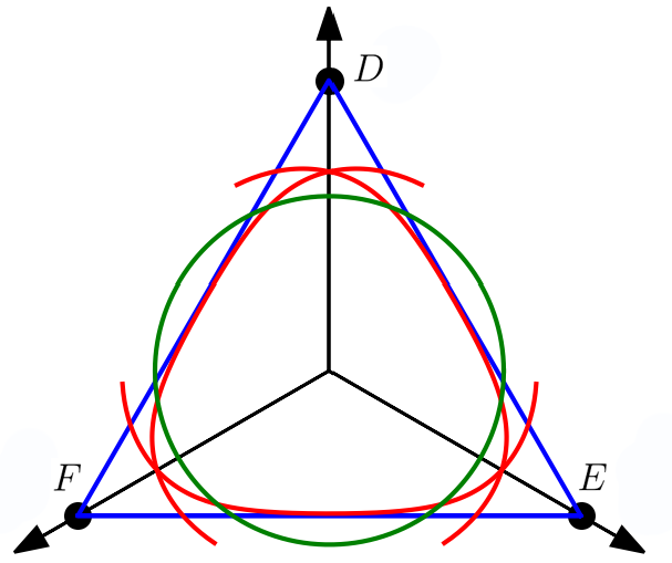
Figure 1: A typical shape of the set of admissible points in the $d+e+f=0$ plane is a intersection of three configurations: a circle (green), a curved-arcs triangle (red) and a line-segments triangle (blue). Points outside the intersection of the triangles refer to non-positive maps. The positivity of maps referring to points in the intersection of the triangles, but outside the circle are not known. Here the values of the parameters are $a=1.7,\leavevmode\nobreak\ b=0.9,\leavevmode\nobreak\ c=0.5$. The interactive graph varying the parameters $\{a,b,c\}$ is available on this link https://github.com/gniewko-s/positive_$3\times 3$_maps_bistochastic_on_diagonal/blob/main/equilateral.py.

IV Decomposability

Let $E_{ij}$ denotes the matrix units in $M_{3}$. Given a linear map $\Phi:M_{3}\to M_{3}$, due to the Choi-Jamiołkowski isomorphism Jam , one can write

$$\hat{\Phi}:=\sum_{i,j=1}^{3}E_{ij}\otimes\Phi(E_{ij})\in M_{3}(M_{3}).$$ (42)

A linear positive map is decomposable if and only if

$$\hat{\Phi}=A+({\rm id}_{3}\otimes{\rm T})B,$$ (43)

with $A,B\geq 0$. Now we provide (non-)decomposability conditions for the map $\Phi_{W}$. Note that proposition 1 implies the following

Corollary 1.

If the map $\Phi_{W}$ is decomposable, then $\Phi_{C}$ is also decomposable. Hence, whenever $\Phi_{C}$ is non-decomposable, then any $W$ compatible with $C$ (in the sense of (33)) gives rise to a non-decomposable map $\Phi_{W}$.

Now, we formulate a necessary and sufficient conditions for decomposability.

Proposition 2.

Suppose that $\Phi_{W}$ is positive but not completely positive. If the following condition holds

$$w_{ij}w_{ji}\geq\left(\frac{\sqrt{(w_{ii}-1)(w_{jj}-1)}-2}{2}\right)^{2},\ \ \ i\neq j,$$ (44)

then the map $\Phi_{W}$ is decomposable.

Proof: We can represent $\hat{\Phi}_{W}$ in the below form (to make the structure of the matrices more transparent we replace $0$ by dots)

$$\hat{\Phi}_{W}=\left(\begin{array}[]{ccc|ccc|ccc}w_{11}-1&.&.&.&-1&.&.&.&-1\\ .&w_{21}&.&.&.&.&.&.&.\\ .&.&w_{31}&.&.&.&.&.&.\\ \hline\cr.&.&.&w_{12}&.&.&.&.&.\\ -1&.&.&.&w_{22}-1&.&.&.&-1\\ .&.&.&.&.&w_{32}&.&.&.\\ \hline\cr.&.&.&.&.&.&w_{13}&.&.\\ .&.&.&.&.&.&.&w_{23}&.\\ -1&.&.&.&-1&.&.&.&w_{33}-1\end{array}\right)=A+({\rm id}_{3}\otimes{\rm T})B,$$ (45)

where the matrices $A$ and $B$ are defined by

$$A=\left(\begin{array}[]{ccc|ccc|ccc}w_{11}-1&.&.&.&a_{12}&.&.&.&a_{13}\\ .&.&.&.&.&.&.&.&.\\ .&.&.&.&.&.&.&.&.\\ \hline\cr.&.&.&.&.&.&.&.&.\\ a_{21}&.&.&.&w_{22}-1&.&.&.&a_{23}\\ .&.&.&.&.&.&.&.&.\\ \hline\cr.&.&.&.&.&.&.&.&.\\ .&.&.&.&.&.&.&.&.\\ a_{31}&.&.&.&a_{32}&.&.&.&w_{33}-1\end{array}\right)\ ,\ \ \ \ B=\left(\begin{array}[]{ccc|ccc|ccc}.&.&.&.&.&.&.&.&.\\ .&w_{21}&.&b_{12}&.&.&.&.&.\\ .&.&w_{31}&.&.&.&b_{13}&.&.\\ \hline\cr.&b_{21}&.&w_{12}&.&.&.&.&.\\ .&.&.&.&.&.&.&.&.\\ .&.&.&.&.&w_{32}&.&b_{23}&.\\ \hline\cr.&.&b_{31}&.&.&.&w_{13}&.&.\\ .&.&.&.&.&b_{32}&.&w_{23}&.\\ .&.&.&.&.&.&.&.&.\end{array}\right),$$ (46)

with

$$a_{ij}=-\frac{1}{2}\sqrt{(w_{ii}-1)(w_{jj}-1)},\ \ \ b_{ij}=\frac{1}{2}\sqrt{(w_{ii}-1)(w_{jj}-1)}-1.$$ (47)

Observe that the conditions (44) imply positivity of both $A$ and $B$. Indeed, $B\geq 0$ if and only if

$$w_{ij}w_{ji}\geq b_{ij}b_{ji}=b_{ij}^{2},$$ (48)

which is equivalent to (44). Positivity of $A$ follows immediately from the positivity of the following $3\times 3$ submatrix

$$\left(\begin{array}[]{ccc}w_{11}-1&a_{12}&a_{13}\\ a_{21}&w_{22}-1&a_{23}\\ a_{31}&a_{32}&w_{33}-1\end{array}\right),$$ (49)

which ends the proof. $\Box$

Proposition 3.

A necessary condition for decomposability of $\Phi_{W}$ reads

$$\sum_{i=1}^{3}w_{ii}+2\sum_{i<j}\sqrt{w_{ij}w_{ji}}\geq 9.$$ (50)

Proof: recall that $\Phi_{W}$ is decomposable if and only if

$${\rm Tr}\,(\hat{\Phi}_{W}X)\geq 0,$$ (51)

for any $X\in M_{3}(M_{3})$ such that $X\geq 0$ together with $({\rm id}_{3}\otimes{\rm T})X\geq 0$. We generalize Størmer approach Stormer-DEC and consider the following matrix $X\in M_{3}(M_{3})$:

$$X=\left(\begin{array}[]{ccc|ccc|ccc}1&.&.&.&1&.&.&.&1\\ .&\epsilon_{1}&.&.&.&.&.&.&.\\ .&.&\frac{1}{\epsilon_{2}}&.&.&.&.&.&.\\ \hline\cr.&.&.&\frac{1}{\epsilon_{1}}&.&.&.&.&.\\ 1&.&.&.&1&.&.&.&1\\ .&.&.&.&.&\epsilon_{3}&.&.&.\\ \hline\cr.&.&.&.&.&.&\epsilon_{2}&.&.\\ .&.&.&.&&.&.&\frac{1}{\epsilon_{3}}&.\\ 1&.&&.&1&.&.&.&1\\ \end{array}\right),$$ (52)

with $\epsilon_{i}>0$. By construction one has $X\geq 0$ and $({\rm id}_{3}\otimes{\rm T})X\geq 0$. One finds

$$\mbox{Tr}(\hat{\Phi}_{W}X)=\sum_{i=1}^{3}w_{ii}+(\epsilon_{1}w_{21}+\frac{1}{\epsilon_{1}}w_{12})+(\epsilon_{2}w_{13}+\frac{1}{\epsilon_{2}}w_{31})+(\epsilon_{3}w_{32}+\frac{1}{\epsilon_{3}}w_{23})-9,$$

and minimization w.r.t. $\{\epsilon_{1},\epsilon_{2},\epsilon_{3}\}$ implies (50). $\Box$

Remark 2.

Let us observe that due to $2\sqrt{w_{ij}w_{ji}}\leq w_{ij}+w_{ji}$ condition (50) implies

$$\sum_{i}w_{ii}+\sum_{i<j}(w_{ij}+w_{ji})=3w\geq 9,$$

and hence $w\geq 3$. It is, therefore, clear that (50) is more restrictive than the interior condition $w\geq 3$. Note that, when $W=C$ (circulant case), then (44) and (50) coincide and reduces to (6).

V Conclusions

In this paper, we generalized the family of positive maps proposed in Korea1 . The generalization consists in relaxing the circulant structure of the matrix $\{C_{ij}\}$, i.e. replacing $C_{ij}$ by $w_{ij}$ satisfying (7). Positivity of such maps is characterized in Theorem 3. The corresponding sufficient and necessary conditions for decomposability are summarized in Propositions 2 and 3, respectively.

It would be interesting to apply this new family of maps for the analysis of the detection of quantum entanglement, where e.g. the so-called optimality property plays a key role Lew ; TOPICAL ; KOREA ; Ha-Kye ; PRA-2022 ; ani1 .

Appendix A Numerical calculations

The code https://github.com/gniewko-s/positive_3x3_maps_bistochastic_on_diagonal/blob/main/equilateral.py is written in the Python language and uses the numpy and matplotlib libraries. It draws on the plane $d+e+f=0$ the following curves being saturations of the following conditions:

• vertex conditions (36) (the blue triangle)

• edge conditions (37 - 39) (the red curved-arcs triangle)

• the hessian positivity condition 35 (the green circle)

• the complete positivity condition 30 (the black shape)

The angles between projections of axes $d$, $e$, $f$ onto the plane are 120^∘.

If $a\geq 1,\leavevmode\nobreak\ b,\leavevmode\nobreak\ c\geq 0$, then the vertex condition (36) cuts off an equilateral triangle on the plane $d+e+f=0$. Its vertices are $(2\mu,-\mu,-\mu)$, $(-\mu,2\mu,-\mu)$, $(-\mu,-\mu,2\mu)$ (denoted $D$, $E$, $F$ respectively). In the function plot we prepare the $x,y$ coordinates of the points of the triangle as follows:

⬇

mu = min(a-1,b,c)

r = 6**.5 * mu

xmax = 3**.5/2*r

x = np.linspace(-xmax,xmax,101)

XV = np.concatenate((x,x))

YV = np.concatenate((-r/2*np.ones(x.shape),r-3**.5*np.abs(x)))

To plot the rest of the listed shapes, we choose the polar coordinate system on the plane centered in the point $d=e=f=0$. We express the Cartesian coordinates $\{d,e,f\}$ by the polar coordinates $\{r,\phi\}$ in the following way:

$$d=\sqrt{\frac{2}{3}}r\cos\phi,\quad e=\sqrt{\frac{2}{3}}r\cos\left(\phi+\frac{2\pi}{3}\right),\quad f=\sqrt{\frac{2}{3}}r\cos\left(\phi-\frac{2\pi}{3}\right),$$ (53)

Now one can rewrite the edge conditions (37) - (39) as:

$$\sqrt{\left(a-1-\frac{r}{\sqrt{6}}\cos\phi\right)^{2}-\frac{r^{2}}{2}\sin^{2}\phi}+\sqrt{\left(\frac{b+c}{2}+\sqrt{\frac{2}{3}}r\cos\phi\right)^{2}-\left(\frac{b-c}{2}\right)^{2}}\geq 1,$$ (54)

$$\sqrt{\left(a-1-\frac{r}{\sqrt{6}}\cos\left(\phi+\frac{2\pi}{3}\right)\right)^{2}-\frac{r^{2}}{2}\sin^{2}\left(\phi+\frac{2\pi}{3}\right)}+\sqrt{\left(\frac{b+c}{2}+\sqrt{\frac{2}{3}}r\cos\left(\phi+\frac{2\pi}{3}\right)\right)^{2}-\left(\frac{b-c}{2}\right)^{2}}\geq 1,$$ (55)

$$\sqrt{\left(a-1-\frac{r}{\sqrt{6}}\cos\left(\phi-\frac{2\pi}{3}\right)\right)^{2}-\frac{r^{2}}{2}\sin^{2}\left(\phi-\frac{2\pi}{3}\right)}+\sqrt{\left(\frac{b+c}{2}+\sqrt{\frac{2}{3}}r\cos\left(\phi-\frac{2\pi}{3}\right)\right)^{2}-\left(\frac{b-c}{2}\right)^{2}}\geq 1.$$ (56)

We obtain the same arcs of a bean curve rotated by $120^{\circ}$, forming a curved-arc triangle. Let us focus on the arc lying antipodal to the point $D$. It spans between angles $[2\pi/3,4\pi/3]$, but due to its symmetry, it is enough to calculate the first half and then mirror the result to the second half.

To obtain the formula for the arc, we proceed as follows. For a given $\phi$ we square twice the arcs equation to get rid of square roots and obtain a four-order polynomial. Next, we calculate its roots and compare which of them is positive and satisfies the original equation (before squaring). If there is no such a root or it is outside the blue triangle, we notice it by putting the value np.NaN for such $\phi$:

⬇

def satisfy_original(a:float,b:float,c:float,phi:float,r:float,tol:float=1e-6) -> bool:

res = ((a-1-r*np.cos(phi))**2 - 3*r**2*np.sin(phi)**2)**.5 + ( ((b+c)/2 + 2*r*np.cos(phi))**2 - ((b-c)/2)**2 )**.5 - 1

return np.abs(res) < tol

def in_triangle(a: float,b: float,c: float,phi: float,r: float) -> bool:

return r <= .5* min(a-1,b,c) / max(-np.cos(phi),-np.cos(phi+2*np.pi/3),-np.cos(phi-2*np.pi/3))

def on_roots(a: float,b: float,c: float,phi: float,roots: np.ndarray) -> float:

roots = [r.real if r.imag == 0 and r>0 and satisfy_original(a,b,c,phi,r) and in_triangle(a,b,c,phi,r) else np.NaN for r in roots]

m = np.nanmin(roots)

return m

def arc_polar(a: float,b: float,c: float) -> Callable[[np.ndarray], np.ndarray]:

def inner(phi: np.ndarray) -> np.ndarray:

coeff4 = 9/4; coeff4 = coeff4*np.ones(phi.shape)

coeff3 = 3*(a+b+c-1) * np.cos(phi)

coeff2 = ((a+b+c-1)**2-4)*np.cos(phi)**2 - 1.5*((a-1)**2-b*c-1)

coeff1 = -((a+b+c-1)*((a-1)**2-b*c-1)+2*(b+c))*np.cos(phi)

coeff0 = ((a-1)**2-b*c-1)**2/4-b*c; coeff0 = coeff0*np.ones(phi.shape)

P = np.array([coeff4,coeff3,coeff2,coeff1,coeff0]).transpose()

P = np.array([on_roots(a,b,c,phii,np.roots(p))*6**.5 for phii, p in zip(phi,P)])

return P

return inner

In this way we calculate an array of the proper values of $r$ for a range of angles $[\pi/3,\pi]$ - twice wider than the halt of the range of the arc. We do it, because the shape we are looking for will be an intersection of areas bounded by arcs and in general we do not know, if for a given $\phi$, the point of the considered arc, or a point of the prolonged neighbouring arc are closer to the origin.

Hence, in the function plot we take the arc prolonged to the twice wider range $[\pi/3,\pi]$, then fold it in the endpoint of the original range, and take the minimum of two values of radius for each $\phi$. In this way we obtain the half of the arc in the considered range. Reflecting it with respect to the value $\pi$, we obtain the arc in the whole range. Next we produce the arrays of $x$-coordinates and $y$-coordinates of points of all three arcs:

⬇

phi = np.linspace(np.pi/3,np.pi,201); r = arc_polar(a,b,c)(phi); # twice prolonged half of arc

r = np.nanmin(np.vstack((r[:101][::-1],r[100:])), axis = 0); # folding prolongation and taking minimum

r = np.hstack((r,r[:0:-1])) # mirror to the second half

phi = np.pi/2 + np.linspace(2*np.pi/3,4*np.pi/3,201) # proper range of phi

XE= np.hstack((r*np.cos(phi), r*np.cos(phi+2*np.pi/3), r*np.cos(phi-2*np.pi/3)))

YE= np.hstack((r*np.sin(phi), r*np.sin(phi+2*np.pi/3), r*np.sin(phi-2*np.pi/3)))

(the shift of the range of the angle by $\pi/2$ is because the axis $d$ points up.)

Next we generate the arrays of $x$ and $y$ coordinates of points of the green circle bounding the set of points representing operators satisfying the hessian condition:

⬇

r = (a+b+c-((a-2*b-2*c)**2+3*(b-c)**2)**.5)/6**.5

XP = r*np.cos(np.linspace(0,2*np.pi,601))

YP= r*np.sin(np.linspace(0,2*np.pi,601))

Finally, to calculate the points of the boundary of the set of completely positive matrices, we transform the saturation of inequality (30) to the form:

$$def+(a-1)(de+ef+fd)+a^{3}-3a^{2}=0$$ (57)

in the polar coordinates:

$$\cos\phi\left(\cos^{2}\phi-\frac{3}{4}\right)\sqrt{\frac{2}{3}}r^{3}-\frac{a-1}{2}r^{2}+a^{2}(a-3)=0.$$ (58)

Here we proceed in a similar fashion as we described for the case of the red curved-arc triangle. For a given $\phi$ we calculate the real, positive roots of the polynomial 58. If such obtained radial coordinate exceeds the radial coordinate of the point on the triangle, then we take the point on the triangle, because complete positivity implies positivity (the set of completely positive maps is a subset of the set of positive maps). The necessary condition for complete positivity is $a\geq 3$, hence otherwise we return an array of np.NaN (empty plot):

⬇

def on_CP_roots(roots: np.ndarray, bound: float):

roots = [(r.real if r < bound else bound) if r.imag == 0 and r>0 else np.NaN for r in roots]

m = np.nanmin(roots)

return m

def CP(a:float, b:float, c:float) -> Callable[[np.ndarray], np.ndarray]:

if a <= 3:

return lambda phi: np.nan * phi

def inner(phi: np.ndarray) -> np.ndarray:

coeff3 = np.cos(phi)*(np.cos(phi)**2-.75) * (2/3)**1.5

coeff2 = -(a-1)/2 * np.ones(phi.shape)

coeff1 = np.zeros(phi.shape)

coeff0 = a**2*(a-3) * np.ones(phi.shape)

P = np.array([coeff3,coeff2,coeff1,coeff0]).transpose()

tri = (1.5**.5 * min(a-1,b,c) / max(-np.cos(phii),-np.cos(phii+2*np.pi/3),-np.cos(phii-2*np.pi/3)) for phii in phi)

P = np.array([on_CP_roots(np.roots(p),bound) for p,bound in zip(P, tri)])

return P

return inner

The above function is then invoked in the function plot to generate the arrays of $x$ and $y$ coordinates:

⬇

phi = np.linspace(0,2*np.pi,601)

r = CP(a,b,c)(phi)

phi = np.pi/2 + phi

XC = r*np.cos(phi)

YC = r*np.sin(phi)

The plots are obtained from the data stored in 1-d arrays XV,YV,XE,YE,XP,YP,XC,YC returned by the function plot.

References

(1) E. Størmer, Positive linear maps of operator algebras, Acta Math. 110, 233 (1963).
(2) E. Størmer, Positive Linear Maps of Operator Algebras,
Springer Monographs in Mathematics (Springer, New York, 2013).
(3) V. Paulsen, Completely Bounded Maps and Operator
Algebras (Cambridge University Press, Cambridge, 2003).
(4) T. Takasaki and J. Tomiyama, On the geometry of positive maps in matrix
algebras, Math. Z. 184, 101 (1983).
(5) J. Tomiyama, On the geometry of positive maps in matrix algebras. II, Linear Algebra Appl. 69, 169 (1985).
(6) K. Tanahashi and J. Tomiyama, Indecomposable positive maps in matrix algebras, Canad. Math. Bull. 31, 308 (1988).
(7) R. Bhatia, Positive Definite Matrices, Princeton series in Applied Mathematics (Princeton University Press, New Jersey, 2007).
(8) R. Horodecki, P. Horodecki, M. Horodecki, and K. Horodecki, Quantum entanglement, Rev. Mod. Phys. 81, 865 (2009).
(9) O. Gühne, and G. Tóth, Entanglement detection, Phys. Rep. 474, 1 (2009).
(10) D. Chruściński and G. Sarbicki, Entanglement witnesses: construction, analysis and classification, J. Phys. A 47, 483001 (2014).
(11) W. A. Majewski and M. Marciniak, On a characterization of positive maps, J. Phys. A: Math. Gen. 34, 5863 (2001).
(12) D. Chruściński and A. Kossakowski, On the structure of entanglement witnesses and new class of positive indecomposable maps, Open Syst. Inf. Dyn. 14, 275 (2007).
(13) D. Chruściński and A. Kossakowski, Spectral conditions for positive maps, Comm. Math. Phys. 290, 1051 (2009).
(14) S.-H. Kye, Facial structures for various notions of positivity and applications to the theory of entanglement, Rev. Math. Phys. 25, 1330002 (2013).
(15) K.-C. Ha and S.-H. Kye, Optimality for indecomposable entanglement witnesses, Phys. Rev. A 86, 034301 (2012).
(16) S. L. Woronowicz, Positive maps of low dimensional matrix algebras, Rep. Math. Phys. 10, 165 (1976).
(17) M.-D. Choi, Completely positive linear maps on complex matrices, Linear Algebra Appl. 10, 285 (1975).
(19) M.-D. Choi, Some assorted inequalties for positive linear maps on -algebras, J. Oper. Theory 4, 271 (1980).
(20) M.-D. Choi and T.-Y. Lam, Extremal positive semidefinite forms, Math. Ann. 231, 1 (1977).
(21) S.-J. Cho, S.-H. Kye, and S. G. Lee, Generalized Choi maps in three-dimensional matrix algebra, Linear Algebra Appl. 171, 213 (1992).
(22) P. Nowosad, Isoperimetric eigenvalue problems in algebras, Comm. Pure Appl. Math. 21, 401 (1968).
(23) S. Yamagami, Cyclic inequalities, Proc. Am. Math. Soc. 118, 521 (1993).
(24) D. Chruściński, M. Marciniak, and A. Rutkowski, Generalizing Choi-Like Maps, Acta Math. Vietnam. 43, 661 (2018).
(25) H. M. Cundy and A. P. Rollett. Mathematical Models, 2nd ed., (Oxford University press, Oxford, New York, 1961).
(26)
A. Jamiołkowski, Linear transformations which preserve trace and positive semidefiniteness of operators, Rep. Math. Phys. 3, 275 (1972).
(27) E. Størmer, Decomposable positive maps on -algebras, Proc. Amer. Math. Sot. 86, 402 (1982).
(28) M. Lewenstein, B. Kraus, J. I. Cirac, and P. Horodecki, Optimization of entanglement witnesses, Phys. Rev. A 62, 052310 (2000).
(29) A. Bera, F. A. Wudarski, G. Sarbicki, and D. Chruściński, Class of Bell-diagonal entanglement witnesses in : Optimization and the spanning property, Phys. Rev. A 105, 052401 (2022).
(30)
A. Bera, G. Sarbicki, D. Chruściński, A class of optimal positive maps in , arXiv:2207.03821.