Red noise in continuous-time stochastic modelling

Abstract

The concept of correlated noise is well-established in discrete-time stochastic modelling but there is no generally agreed-upon definition of the notion of red noise in continuous-time stochastic modelling. Here we discuss the generalization of discrete-time correlated noise to the continuous case. We give an overview of existing continuous-time approaches to model red noise, which relate to their discrete-time analogue via characteristics like the autocovariance structure or the power spectral density. The implications of carrying certain attributes from the discrete-time to the continuous-time setting are explored while assessing the inherent ambiguities in such a generalization. We find that the attribute of a power spectral density decaying as $S(\omega)\sim\omega^{-2}$ commonly ascribed to the notion of red noise has far reaching consequences when posited in the continuous-time stochastic differential setting. In particular, any Itô-differential $\mathrm{d}Y_{t}=\alpha_{t}\mathrm{d}t+\beta_{t}\mathrm{d}W_{t}$ with continuous, square-integrable integrands must have a vanishing martingale part, i.e. $\mathrm{d}Y_{t}=\alpha_{t}\mathrm{d}t$ for almost all $t\geq 0$. We further argue that $\alpha$ should be an Ornstein-Uhlenbeck process.

1 Introduction

In many fields of dynamical modelling, it is common practice to introduce an additive stochastic term to incorporate unresolved dynamics into the otherwise deterministically defined equation of discrete-time evolution. A simple example of this may be a stochastic process defined by

$$X_{k+1}-X_{k}=f(X_{k},k)+\sigma\varepsilon_{k},\,X_{0}=x_{0}\in\mathbb{R}.$$ (1)

In the classical setting, the noise term $\varepsilon_{k}$ will for each time-step be an independent standard Gaussian random variable [1]. However, in some cases it may be imperative to discard this assumption of independence, for instance if the unresolved dynamics are suspected to exhibit persistence in time [2, 3]. Perhaps the most common example of such correlated noise is so-called red noise, generated via an AR(1)-process:

$$\varepsilon_{k+1}=\varphi\varepsilon_{k}+z_{k},\,\varepsilon_{0}\sim\mathcal{N}\left(0,(1-\varphi^{2})^{-1}\right),$$ (2)

where $0<\varphi<1$ and now the $(z_{k})_{k\in\mathbb{N}}$ are i.i.d. standard Gaussian. The initial distribution of $\varepsilon_{0}$ is chosen specifically such that the process $\varepsilon$ is stationary in the weak sense. Each instance $\varepsilon_{k}$ of the discrete-time noise process $\varepsilon$ has exponentially decaying correlation to its neighboring instances

$$R_{\varepsilon}(\tau) =\frac{\varphi^{\left|\tau\right|}}{1-\varphi^{2}},\,\tau\in\mathbb{N}$$ (3)

and this particular noise process is the basis for many applied discrete-time stochastic models [4, 5, 6, 7].

When modelling natural systems, however, it is often more rigorous to model their dynamics in continuous time. Incorporating the concept of noise into such models requires delicate mathematical constructions. The field of stochastic analysis offers a wide range of possibilities for introducing stochasticity into continuous-time dynamics. Discrete-time dynamics with additive noise, in similar spirit of (1), may be modelled by the following stochastic differential equation (SDE):

$$\mathrm{d}X_{t}=f(X_{t},t)\mathrm{d}t+\sigma\mathrm{d}Y_{t},\,X_{0}=x_{0}\in\mathbb{R}.$$ (4)

In the classical setting of uncorrelated noise, $Y=(Y_{t})_{t\in\mathbb{R}_{+}}$ takes the form of a Wiener process $W=(W_{t})_{t\in\mathbb{R}_{+}}$ and the equation should be understood as an equation of Itô-integrals. A wide class of processes $Y$ which may replace $W$ and still result in a well-defined equation of Itô-integrals is the class of Itô-processes

$$Y_{t}=Y_{0}+\int_{0}^{t}\alpha_{s}\mathrm{d}s+\int_{0}^{t}\beta_{s}\mathrm{d}W_{s},$$

for suitable processes $\alpha=(\alpha_{t})_{t\in\mathbb{R}_{+}}$ and $\beta=(\beta_{t})_{t\in\mathbb{R}_{+}}$.

The aim of this work is to bridge the dichotomy between concepts of correlated noise stemming from discrete-time models of the form (1) and the possible continuous-time adaptations in the fashion of SDEs like (4). While the Euler-Mayurama method offers a consistent way of translating the latter to the former, such a translation is decidedly not unique for the diametric task. We claim to be able to reduce the number of possible continuous-time constructions under certain assumptions. In a first step, we will invoke the Markov-property of the AR(1)-process in (2) to search for a corresponding continuous-time process (Section 2). Thereafter, we will focus on spectral characteristics (Section 3). Alternatives will be considered in Sections 4 and 6 and an example will be presented in Section 5.

2 Red noise as a stationary Gaussian Markov-process

Starting from the discrete-time formulation of the red noise process in equation (2), we can make a strong case for a specific continuous-time analogue: Suppose $(\varepsilon_{k})_{k\in\mathbb{N}}$ is a sub-sample of a stationary, measurable process $\alpha=(\alpha_{t})_{t\in\mathbb{R}_{+}}$ at integer time-steps. Then, if one requires that $\alpha$ is a Gaussian Markov process in continuous time in the same manner as $\varepsilon$ is a Gaussian Markov process in discrete time, $\alpha$ has to be an Ornstein-Uhlenbeck process. This is because all stationary, measurable processes which are simultaneously Gaussian and Markov are of the Ornstein-Uhlenbeck type (Theorem 1.1 in [8]). Therefore, a distinctly motivated continuous-time analogue of (1) would be

$$\mathrm{d}X_{t}=f(X_{t},t)\mathrm{d}t+\alpha_{t}\mathrm{d}t.$$

Discretizing this via the Euler method with integration step $\Delta t=1$ would result in the original equation (1). While we will later argue for the same continuous-time red noise model, this derivation is not entirely satisfactory. The a priori restriction $\mathrm{d}Y_{t}=\alpha_{t}\mathrm{d}t$ we have made before arguing for any specific process $\alpha$ is rather narrow considering the wide range of possibilities offered in stochastic calculus and it is not directly motivated from any characteristic of discrete-time red noise. In fact, there is an inherent ambiguity which cannot be resolved from the standpoint of a single discrete-time dynamic equation, i.e. without knowledge about how the equation scales when the integration time-step $\Delta t=1$ changes. The assumption we have made here, namely that the discrete-time noise term for any choice of $\Delta t>0$ should be $\varepsilon_{k}^{(\Delta t)}=\alpha_{k}\Delta t$, essentially implies that the autocovariance structure of the discrete-time noise should scale uniformly with a factor of $(\Delta t)^{2}$. This is decidedly not the case for uncorrelated noise $z_{k}^{(\Delta t)}$, where the variance classically scales with a factor of $\Delta t$ to ensure a convergence to the white-noise differential $\mathrm{d}W_{t}$. However, there exists a characteristic which can be deduced from observations, enjoys precedent in application, and elegantly implies a certain scaling-behaviour of the discrete-time differential equation. This characteristic will be a vanishing power spectral density in the limit of infinitely high frequencies.

3 Characterization via the power spectral density

Throughout this section we will work on a filtered probability space $(\Omega,\mathcal{F},(\mathcal{F}_{t})_{t\in\mathbb{R}_{+}},\mathbb{P})$ supporting a Brownian motion $W=(W_{t})_{t\in\mathbb{R}_{+}}$. For any $Y_{0}\in\mathcal{F}_{0}$ and predictable processes $\alpha=(\alpha_{t})_{t\in\mathbb{R}_{+}}$ and $\beta=(\beta_{t})_{t\in\mathbb{R}_{+}}$ the Itô-process

$$Y_{t}=Y_{0}+\int_{0}^{t}\alpha_{s}ds+\int_{0}^{t}\beta_{s}dW_{s},\ t\geq 0,$$

is well-defined if e.g. the integrability condition

$$\int_{0}^{T}\mathbb{E}\left[\alpha_{t}^{2}+\beta_{t}^{2}\right]\mathrm{d}t<\infty\text{ for all }T>0$$ (5)

is satisfied. The power spectral density (PSD) of $\mathrm{d}Y$ is defined as

$$S_{\mathrm{d}Y}(\omega):=\lim_{T\rightarrow\infty}\mathbb{E}\left[\frac{1}{T}\left|\int_{0}^{T}\exp(-i\omega t)\mathrm{d}Y_{t}\right|^{2}\right],$$

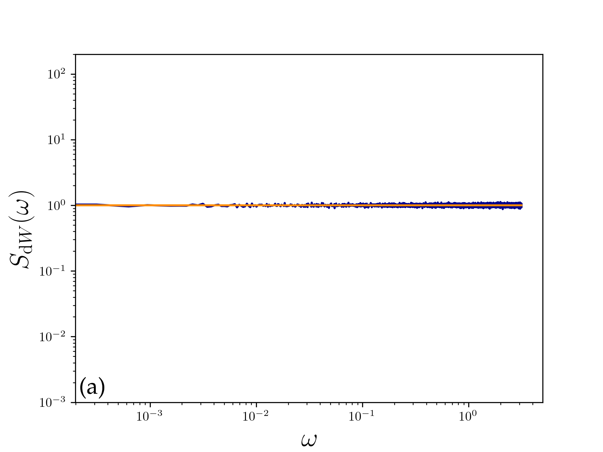
if the limit exists. One immediate result via the Itô-isometry is $S_{\mathrm{d}W}\equiv 1$.

If $\mathrm{d}Y_{t}=\alpha_{t}\mathrm{d}t$ for some stationary, centered and square-integrable process $\alpha$ with absolutely integrable autocovariance structure $R_{\alpha}(\tau)$, then the Wiener-Khinchin theorem applies:

$$S_{\alpha_{t}\mathrm{d}t}(\omega)=\mathcal{F}[R_{\alpha}(\tau)](\omega):=\int_{-\infty}^{\infty}\exp(-i\omega\tau)R_{\alpha}(\tau)\mathrm{d}\tau.$$

In most applications of correlated noise, the properties of the PSD are more prominently featured than the autocovariance counterpart. In fact, the name red noise stems from the observation that low frequencies exhibit the largest amplitudes in the PSD. A sufficient but not equivalent condition for this is to demand an asymptotically vanishing spectral density, i.e. $S(\omega)\rightarrow 0$ as $\omega\rightarrow 0$. In much of the applied literature on this topic, a rate of decay of $\mathcal{O}(\omega^{-2})$ is taken to be the defining characteristic of red noise [9, 10, 11] and the noise instances are sometimes constructed directly via its PSD [12, 13, 14]. This particular dependence on $\omega$ can either be derived from observations or motivated by again assuming that the process $\alpha$ has the autocovariance structure given in (3) and calculating the implied PSD of this process:

$$S_{\alpha_{t}\mathrm{d}t}(\omega)=\mathcal{F}[R_{\alpha}(\tau)](\omega)=\frac{-2\log(\varphi)}{(1-\varphi^{2})(\log(\varphi)^{2}+\omega^{2})}=\mathcal{O}(\omega^{-2}).$$

Note that we have not quite resolved the ambiguity of how the autocovariance structure should scale with the integration time-step but have instead invoked a stronger definition of red noise on the side of the PSD, namely that it vanishes in the high-frequencies limit. With this stronger definition, we are now able to formulate our main result, heavily constraining the possible choices of continuous-time red noise equivalents that are modelled through an Itô-differential.

Theorem.

Let $\alpha$ and $\beta$ be adapted processes satisfying the integrability condition (5). Suppose that $\alpha$ has continuous paths and $\beta$ is predictable. Define the Itô-process

$$Y_{t}=\int_{0}^{t}\alpha_{s}\mathrm{d}s+\int_{0}^{t}\beta_{s}\mathrm{d}W_{s},\quad t\geq 0.$$

1. Finite time horizon. Assume that the finite-time PSD of $\mathrm{d}Y$ vanishes in the limit of infinitely high frequencies, i.e.

$$S^{(T)}_{\mathrm{d}Y}(\omega):=\mathbb{E}\left[\frac{1}{T}\left|\int_{0}^{T}\exp(-i\omega t)\mathrm{d}Y_{t}\right|^{2}\right]\xrightarrow[\omega\to\infty]{}0.$$

Then $\beta_{t}=0$ $\mathbb{P}$-a.s. for almost all $t\in[0,T]$.

2. Infinite time horizon. Assume that $\alpha$ and $\beta$ are stationary processes and let $\alpha$ be centered around $0$ with an absolutely integrable autocovariance structure $R_{\alpha}(\tau)$. Assume that the PSD of $\mathrm{d}Y$ on an infinite time horizon exists. If the PSD of $\mathrm{d}Y$ vanishes in the limit of infinitely high frequencies, i.e.

$$S_{\mathrm{d}Y}(\omega)\xrightarrow[\omega\to\infty]{}0,$$

then $\beta_{t}=0$ $\mathbb{P}$-a.s. for all $t\geq 0$.

We refer to Appendix A.1 for a proof of this theorem. If one objective of finding a suitable red noise Itô-differential $\mathrm{d}Y$ is to have it exhibit a vanishing PSD in the limit of infinitely high frequencies, then all reasonable choices necessarily have the form $\mathrm{d}Y_{t}=\alpha_{t}\mathrm{d}t$. The range of reasonable choices defined through the conditions on $\alpha$ and $\beta$ in the theorem is narrower if one examines an infinite time horizon, since asymptotic behaviour needs to be taken into account. The strict stationarity condition for $\alpha$ and $\beta$ may be replaced by other suitable constraints on their asymptotic behaviour. In the finite time horizon case, the restrictions on $\alpha$ and $\beta$ reduce to being square-integrable together with the path-continuity of $\alpha$, which may be motivated from physical principles.

Taking into account the arguments on Gaussian Markov processes from the last section, we may conclude that the Ornstein-Uhlenbeck process $U$ defined by

$$\mathrm{d}U_{t}=-\theta U_{t}\mathrm{d}t+\mathrm{d}W_{t},\,U_{0}\sim\mathcal{N}\left(0,\frac{1}{2\theta}\right)$$

constitutes a unique way of modelling red noise in continuous time via

$$\mathrm{d}Y_{t}=\alpha_{t}\mathrm{d}t=U_{t}\mathrm{d}t$$

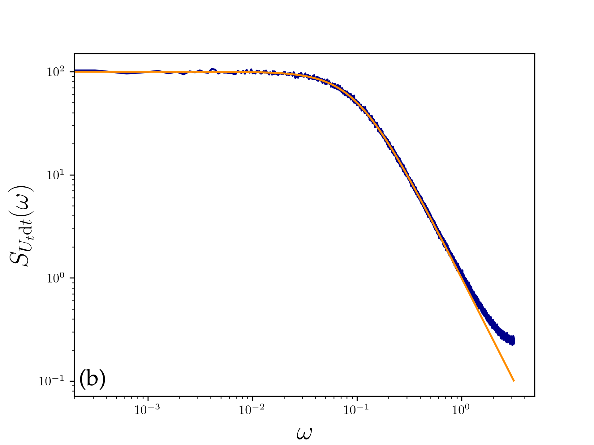
The Ornstein-Uhlenbeck process $U$ exhibits both the property of exponentially decaying autocovariance and the $\mathcal{O}(\omega^{-2})$ decay of the PSD of the differential $U_{t}\mathrm{d}t$ that we are accustomed to from the discrete-time case (see Figure 1b for an illustration and Appendix A.2 for a derivation):

$$R_{U}(\tau) =\frac{1}{2\theta}\exp(-\theta\left|\tau\right|)$$

$$S_{U_{t}\mathrm{d}t}(\omega) =\frac{1}{\theta^{2}+\omega^{2}}$$

With the condition of a vanishing PSD in the high-frequency limit, there will be no structurally different reasonable choices of continuous-time red noise models. This model is featured in some of the applied literature [15, 16, 17, 18], but to the best of our knowledge no comprehensive justification has hitherto been brought forth in its favour.

4 Alternatives under weaker assumptions

In case that red noise should only have to exhibit strong amplitudes in low frequencies, but not necessarily a vanishing PSD at $\omega\rightarrow\infty$, we are again left with the aforementioned ambiguity of scaling in the autocovariance structure. For correlated noise with this relaxed definition, we propose one notable construction: Given a Brownian motion $W$ we consider the SDE system

$$\mathrm{d}U_{t} =-\theta U_{t}\mathrm{d}t+\mathrm{d}W_{t},$$

$$\mathrm{d}Y_{t} =\gamma U_{t}\mathrm{d}t+\mathrm{d}W_{t}.$$

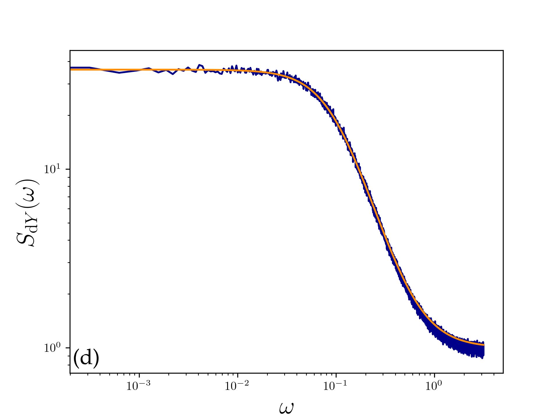
In this case, the PSD is (see Appendix A.2 and Fig. 1d)

$$S_{\mathrm{d}Y}(\omega)=\frac{(\gamma+\theta)^{2}+\omega^{2}}{\theta^{2}+\omega^{2}}.$$

If $\gamma>0$, the condition of decaying PSD toward higher frequencies is satisfied, but the limit for large frequencies is not 0:

$$S_{\mathrm{d}Y}(\omega)\xrightarrow[\omega\to\infty]{}1.$$

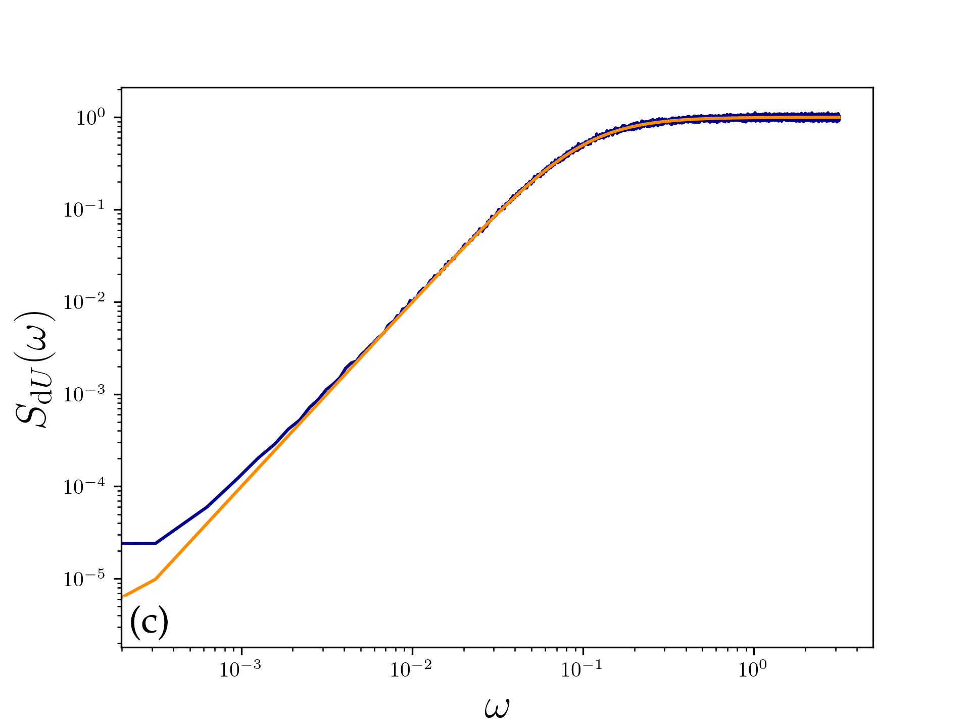
For $-2\theta<\gamma<0$ however, the results are different. One special case of this bears mentioning, since it is at times proposed in the literature as a continuous time red noise model [19, 7, 20]. For $\gamma=-\theta$, we have $\mathrm{d}Y=\mathrm{d}U$ and it may seem conceptually appealing to label this red noise. However, the PSD of $\mathrm{d}U$ exhibits the opposite of what we have so far understood as red noise characteristics:

$$S_{\mathrm{d}U}=\frac{\omega^{2}}{\theta^{2}+\omega^{2}}.$$

For low frequencies, $S_{\mathrm{d}U}$ tends to 0 and it is monotonically increasing in $\omega$ (see Figure 1c). The discrete-time noise terms resulting from discretizing such a differential via the Euler-Mayurama method at integration time-step $\Delta t$ would also be negatively correlated (here $\tau\geq\Delta t$):

$$\mathrm{Cov}\left(U_{\Delta t}-U_{0},U_{\tau+\Delta t}-U_{\tau}\right)=\frac{1}{\theta}\exp(-\theta\tau)(1-\cosh(\theta\Delta t))<0.$$

The usage of $\mathrm{d}U$ in this context constitutes a common misconception about the formulation of continuous-time stochastic models from desired discrete-time characteristics. If one posits a certain distribution or correlation in the noise component of a system and encounters the desired property in a stochastic process $V$, then the differential $\mathrm{d}V$ is in general not a suitable noise term since it may exhibit entirely different properties. In [19] and [7], this would instead imply using $V_{t}\mathrm{d}t$. Even when introducing $\mathrm{d}U$ more generally as coloured noise [21, 22], one should be aware of the conceptual implications of negative correlation. If the aim of introducing correlation is to model temporal persistence in the noise forcing, then this would heuristically always call for positive correlation.

Figure 1: The theoretically computed (orange) and observed (blue) PSD for each of the discussed noise differentials, shown on a log-log-scale. The observed PSD was obtained by taking the squared absolute value of the Fourier-transformed noise signal and subsequently averaging over $10^{3}$ neighbouring frequencies respectively. The length of the sample was $2\cdot 10^{7}$, which implies a total of $10^{7}$ analyzed frequencies and $10^{4}$ after averaging. (a) PSD of unit white noise $\mathrm{d}W$. (b) PSD of the red noise differential $U_{t}\mathrm{d}t$. The characteristic $\omega^{-2}$ asymptotic can be empirically observed until close to the Nyquist frequency, at which point the discrete nature of the data skews the PSD. (c) PSD of the differential $\mathrm{d}U$ sometimes erroneously referred to as red noise. (d) PSD of the red noise alternative $\mathrm{d}Y_{t}=\gamma U_{t}\mathrm{d}t+\mathrm{d}W_{t}$, $\gamma>0$, when allowing for a non-vanishing PSD at $\omega\rightarrow\infty$. Parameter values where chosen as $\theta=0.1$ and $\gamma=0.5$.

5 Example: Linearly restoring process

Apart from potentially being a more accurate modelling approach, the continuous-time realm also allows for the use of more advanced methods from stochastic analysis in the search of analytical solutions. We can observe this for the case of an AR(1) process whose noise term is itself an AR(1) process:

$$X^{(d)}_{k+1} =\psi X^{(d)}_{k}+\sigma\varepsilon_{k},\,X^{(d)}_{0}=x_{0}\in\mathbb{R}$$

$$\varepsilon_{k+1} =\varphi\varepsilon_{k}+z_{k},\,\varepsilon_{0}=0$$

Following our previous reasoning, we propose that

$$\mathrm{d}X^{(c)}_{t} =-\lambda X^{(c)}_{t}\mathrm{d}t+\sigma U_{t}\mathrm{d}t,\,X^{(c)}_{0}=x_{0}\in\mathbb{R}$$

$$\mathrm{d}U_{t} =-\theta U_{t}\mathrm{d}t+\mathrm{d}W_{t},\,U_{0}=0$$

with $\lambda:=-\log(\psi)$ and $\theta:=-\log(\varphi)$ is a consistent continuous-time analogue that captures the essence of the discrete-time model and its noise characteristics. This allows us to solve for the Gaussian process

$$X^{(c)}_{t}=x_{0}\exp(-\lambda t)+\sigma\int_{0}^{t}\exp(-\lambda(t-s))U_{s}\mathrm{d}s$$

and its asymptotically stationary autocorrelation structure

$$r_{X^{(c)}}(\tau)\asymp\sigma^{2}\frac{\lambda\exp(-\theta\left|\tau\right|)-\theta\exp(-\lambda\left|\tau\right|)}{\lambda-\theta}.$$ (6)

It is in principle possible to obtain similar results in the discrete-time realm by computing the first and second moment of $X^{(d)}_{k}$ in the stationary limit via infinite series analysis. Performing the calculations in the continuous-time realm, however, makes them both more feasible and more robust. An interesting observation is that the asymptotic distribution of the resulting process $X^{(c)}$ remains identical after interchanging the values of $\lambda$ and $\theta$ in the set of the generating differential equations.
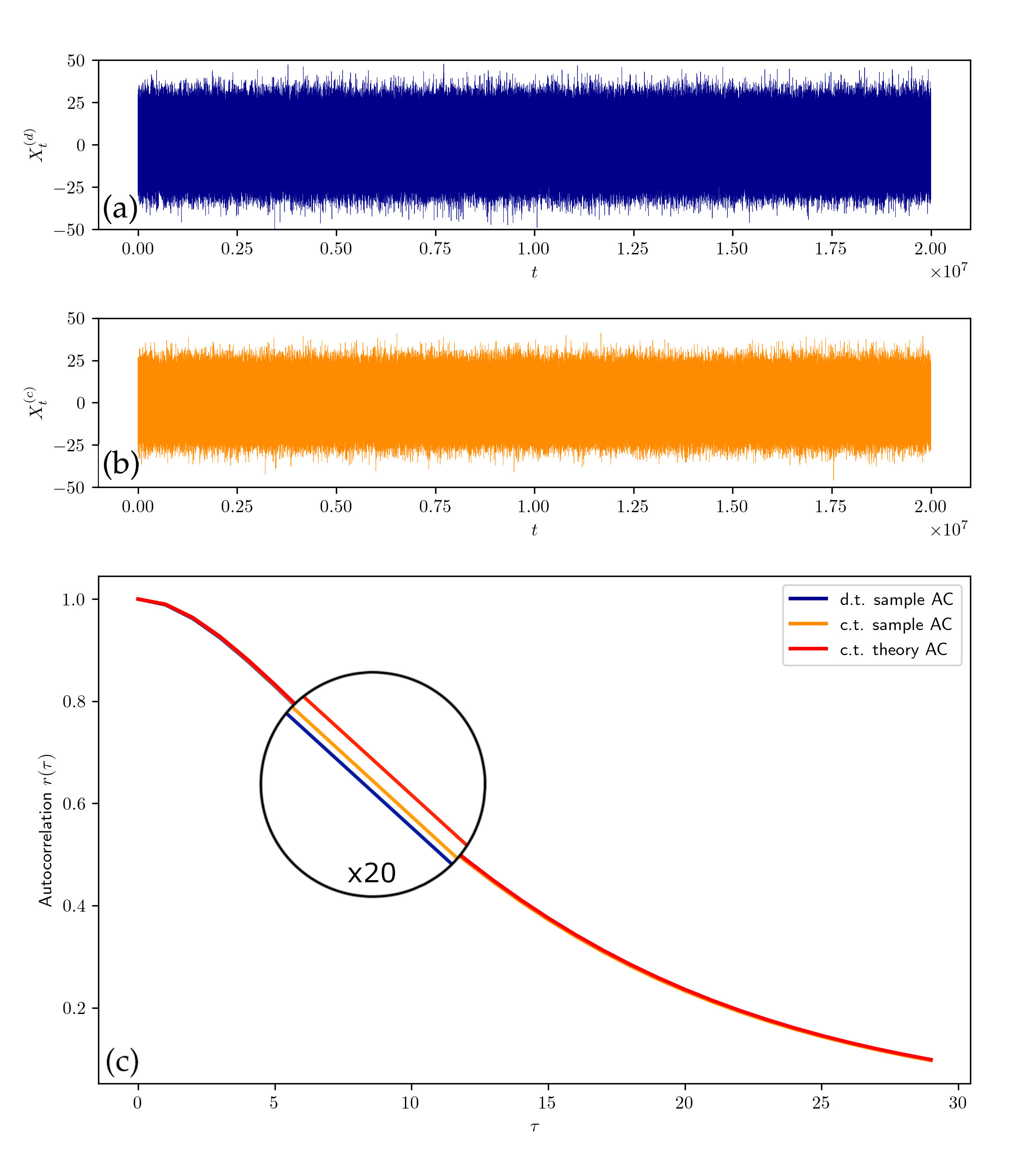
We illustrate the efficacy of the continuous-time modelling approach by sampling both $X^{(d)}$ and $X^{(c)}$ and comparing their observed autocorrelation structure with the theoretically derived autocorrelation structure in equation (6) (see Figure 2). When integrating the continuous-time stochastic differential equations for $X^{(c)}$ it is imperative to minimize the errors introduced by numerical discretization. This is possible via the following discrete-time representation of the Ornstein-Uhlenbeck process $U$.
Define for a time-step $\delta t$ the AR(1) process

$$q_{k+1}=\exp(-\theta\delta t)q_{k}+\frac{1}{\sqrt{2\theta}}\left(1-\exp(-2\theta\delta t)\right)^{1/2}z_{k},\quad q_{0}\sim\mathcal{N}\left(0,\frac{1}{2\theta}\right),$$

where the $z_{k}$ are i.i.d. unit Gaussian. Then we have

$$(q_{k})_{k=0,\dots,K-1}\overset{d}{=}(U_{k\delta t})_{k=0,\dots,K-1},$$

meaning they have the same $K$-dimensional marginals. This may be used to integrate continuous-time equations involving the Ornstein-Uhlenbeck process with minimal loss of accuracy in distribution through discretization. Now sampling $X^{(c)}$ at time-steps $\Delta t>0$ can be achieved by first generating $U$ at time-steps $\delta t\ll\Delta t$, integrating $\mathrm{d}X^{(c)}$ via the Euler-method at steps $\delta t$ and subsequently sampling the result at steps $\Delta t$.

Figure 2: (a) A sample path of $X^{(d)}$ and (b) a sample path of $X^{(c)}$. (c) Their respective estimated autocorrelation structure plotted in blue and orange. The theoretical autocorrelation structure (see eq. (6)) of the continuous-time model is plotted in red for comparison. The realization of the discrete-time equations was computed directly from the sampled unit normals $(z_{k})$. For the continuous-time equations, we sampled $U$ at intervals of $\delta t=10^{-1}$, integrated the equation for $X^{(c)}$ via the Euler method and subsequently sampled every $10$th value of the resulting time series as described in the main text. The length of the considered time series is $2\cdot 10^{7}$ each. The estimated and theoretical autocorrelation structures do not exhibit significant differences (within $1$%). Parameter values were chosen to be $\psi=0.8$, $\varphi=0.9$ and $\sigma=1$.

6 Beyond the Itô-framework of stochastic integration

In many applied fields of stochastic modelling, the possibility of using self-similar processes like fractional Brownian motion $B^{H}_{t}$ with Hurst parameter $H\neq 1/2$ in lieu of semimartingales for modelling noise has gained great popularity in applications, cf. e.g. [23, 24]. The non-stationary autocovariance ($\tau\geq 0$)

$$R_{B^{H}}(t,\tau)=\frac{1}{2}(t^{2H}+(t+\tau)^{2H}-\tau^{2H})$$

implies stationary increments $B^{H}_{t+\Delta t}-B^{H}_{t}\sim\mathcal{N}(0,\Delta t^{2H})$ which are positively correlated if and only if $H>1/2$. This so-called long memory case is interesting to us because it allows for the modelling of persistence in the noise increments. Since the paths of $B^{H}$ have vanishing $p$-variation for any $p>H^{-1}$, the class of admissible integrand processes $\nu$ in the Young-framework of integration is quite large: If the paths of $\nu$ possess finite $2$-variation, then the pathwise Riemann-Stieltjes integral is well-defined. It is therefore sensible to consider stochastic dynamical systems in the form of integral equations where some terms are integrated with respect to fractional Brownian motion. Extensive and rigorous theory on this topic may be found in [25]. A consistent derivation of the PSD associated with the differential $\mathrm{d}B^{H}_{t}$, often referred to as fractional Gaussian noise, is given in [26]:

$$S_{\mathrm{d}B^{H}_{t}}(\omega)=C_{H}\omega^{1-2H},$$

where $C_{H}$ is a constant depending only on $H$. Hence the differential exhibits a vanishing PSD in the limit of high frequencies and may generally be considered as an alternative continuous-time modelling approach for the concept of red noise. However, the persistence of fractional Gaussian noise in terms of its autocovariance only decays with $\mathcal{O}(\tau^{2H-2})$, in contrast to the usual exponential decay seen in discrete-time red noise. This should give pause for concern when we consider to use fractional Gaussian noise as a continuous-time red noise term. Fractional Gaussian noise is instead often referred to as a long-memory noise term [27, 28, 29] in analogy to its continuous-time origin.

Appendix A Appendix

A.1 Proof of the Theorem

1. Finite time horizon. First, we show that the constant term in the finite-time PSD stemming from the $\beta_{t}\mathrm{d}W_{t}$ term must be matched by the PSD of $\alpha_{t}\mathrm{d}t$ in order to result in an overall PSD which is vanishing at $\omega\rightarrow\infty$.

$$S^{(T)}_{\mathrm{d}Y}(\omega) =\mathbb{E}\left[\frac{1}{T}\left|\int_{0}^{T}\exp(-i\omega t)\mathrm{d}Y_{t}\right|^{2}\right]$$

$$=\mathbb{E}\left[\frac{1}{T}\left|\int_{0}^{T}\exp(-i\omega t)\alpha_{t}\mathrm{d}t+\int_{0}^{T}\exp(-i\omega t)\beta_{t}\mathrm{d}W_{t}\right|^{2}\right]$$

$$=\frac{1}{T}\left\lVert\int_{0}^{T}\exp(-i\omega t)\alpha_{t}\mathrm{d}t+\int_{0}^{T}\exp(-i\omega t)\beta_{t}\mathrm{d}W_{t}\right\rVert_{L^{2}(\Omega)}^{2}$$

$$\geq\left[\frac{1}{\sqrt{T}}\left\lVert\int_{0}^{T}\exp(-i\omega t)\alpha_{t}\mathrm{d}t\right\rVert_{L^{2}(\Omega)}-\frac{1}{\sqrt{T}}\left\lVert\int_{0}^{T}\exp(-i\omega t)\beta_{t}\mathrm{d}W_{t}\right\rVert_{L^{2}(\Omega)}\right]^{2}$$

$$=\left(\sqrt{S^{(T)}_{\alpha_{t}\mathrm{d}t}(\omega)}-\sqrt{\frac{1}{T}\int_{0}^{T}\mathbb{E}\left[\beta_{t}^{2}\right]\mathrm{d}t}\right)^{2},$$

where we used the inverse triangle inequality. Since we assumed $S^{(T)}_{\mathrm{d}Y}(\omega)\xrightarrow[\omega\to\infty]{}0$, we conclude

$$S^{(T)}_{\alpha_{t}\mathrm{d}t}(\omega)\xrightarrow[\omega\to\infty]{}\frac{1}{T}\int_{0}^{T}\mathbb{E}\left[\beta_{t}^{2}\right]\mathrm{d}t.$$

It remains to prove that this limit is $0$. Since we have uniform integrability of the random variables $\int_{0}^{T}\exp(-i\omega t)\alpha_{t}\mathrm{d}t$ for all choices of $\omega\in\mathbb{R}$ via

$$\left\lVert\int_{0}^{T}\exp(-i\omega t)\alpha_{t}\mathrm{d}t\right\rVert_{L^{2}(\Omega)}\leq\int_{0}^{T}\left\lVert\alpha_{t}\right\rVert_{L^{2}(\Omega)}\mathrm{d}t<\infty,$$

it suffices to prove that

$$\int_{0}^{T}\exp(-i\omega t)\alpha_{t}\mathrm{d}t\xrightarrow[\omega\rightarrow\infty]{a.s.}0.$$ (7)

But each path $a:[0,T]\rightarrow\mathbb{R}$ of $\alpha$ is uniformly continuous on the compact domain, so for any $\epsilon>0$, we find a $\delta_{\epsilon}>0$ such that for $\omega>\omega_{\epsilon}:=2\pi/\delta_{\epsilon}$ we may estimate

$$\left|\int_{t_{0}}^{t_{0}+\delta_{\epsilon}}\cos(\omega t)a(t)\mathrm{d}t\right|\leq\frac{\epsilon}{2}\int_{t_{0}}^{t_{0}+\delta_{\epsilon}}\left|\cos(\omega t)\right|\mathrm{d}t.$$

for all $t_{0}\in[0,T-\delta_{\epsilon}]$. So the real part of the integral in question becomes arbitrarily small for large $\omega>\omega_{\epsilon}$:

$$\left|\int_{0}^{T}\cos(\omega t)a(t)\mathrm{d}t\right|\leq\frac{\epsilon}{2}\int_{0}^{T}\left|\cos(\omega t)\right|\mathrm{d}t\leq\frac{\epsilon}{2}T.$$

The real part and similarly the imaginary part of (7) converge to $0$ for every path of $\alpha$. Hence the limit in question is also $0$:

$$S^{(T)}_{\alpha_{t}\mathrm{d}t}(\omega)\xrightarrow[\omega\to\infty]{}0=\frac{1}{T}\int_{0}^{T}\mathbb{E}\left[\beta_{t}^{2}\right]\mathrm{d}t.$$

We may conclude that for almost all $t\in[0,T]$ we have $\beta_{t}=0$ $\mathbb{P}$-almost surely.

2. Infinite time horizon. By identical arguments as in the first part of the proof, we arrive at

$$S_{\alpha_{t}\mathrm{d}t}(\omega):=\lim_{T\rightarrow\infty}\mathbb{E}\left[\frac{1}{T}\left|\int_{0}^{T}\exp(-i\omega t)\alpha_{t}\mathrm{d}t\right|^{2}\right]\xrightarrow[\omega\to\infty]{}\lim_{T\rightarrow\infty}\frac{1}{T}\int_{0}^{T}\mathbb{E}\left[\beta_{t}^{2}\right]\mathrm{d}t=\mathbb{E}\left[\beta_{0}^{2}\right],$$

on the condition that the limit of $T\rightarrow\infty$ in the above definition of $S_{\alpha_{t}\mathrm{d}t}$ exists. Because $\alpha$ is square-integrable, its autocovariance $R_{\alpha}(\tau)$ is bounded by $\mathrm{Var}\left(\alpha_{0}\right)$ for all $\tau\in\mathbb{R}$. This, together with the absolute integrability of $R_{\alpha}$ implies that $R_{\alpha}\in L^{2}(\mathbb{R})$. By the Wiener-Khinchin theorem and Plancherel’s theorem, we deduce

$$S_{\alpha_{t}\mathrm{d}t}=\mathcal{F}[R_{\alpha}]\in L^{2}(\mathbb{R})$$

and thereby confirm that the limit in the definition of $S_{\alpha_{t}\mathrm{d}t}$ exists. We have established that $S_{\alpha_{t}\mathrm{d}t}$ converges to a constant as $\omega\rightarrow\infty$. In order for $S_{\alpha_{t}\mathrm{d}t}$ to be square-integrable, the constant in question must be $0$. Hence, we must have

$$\mathbb{E}\left[\beta_{t}^{2}\right]=\mathbb{E}\left[\beta_{0}^{2}\right]=0$$

which implies $\beta_{t}=0$ $\mathbb{P}$-a.s. for all $t\geq 0$.

∎

A.2 Derivation of the power spectral densities

For unit white noise $\mathrm{d}W$, the calculation is a straightforward application of the Itô-isometry:

$$S_{\mathrm{d}W}(\omega)=\lim_{T\rightarrow\infty}\mathbb{E}\left[\frac{1}{T}\left|\int_{0}^{T}\exp(-i\omega t)\mathrm{d}W_{t}\right|^{2}\right]=\lim_{T\rightarrow\infty}\mathbb{E}\left[\frac{1}{T}\int_{0}^{T}1\mathrm{d}t\right]=1$$

For the other claims, first define the Ornstein-Uhlenbeck process via the SDE

$$\mathrm{d}U_{t}=-\theta U_{t}\mathrm{d}t+\mathrm{d}W_{t},\quad U_{0}\sim\mathcal{N}\left(0,\frac{1}{2\theta}\right),$$

so that $U$ is stationary with autocovariance $\mathrm{Cov}\left(U_{t},U_{t+\tau}\right)=\frac{1}{2\theta}\exp(-\theta\left|\tau\right|)$ and compute via the Fubini-Tonelli Theorem

$$S_{U_{t}\mathrm{d}t}(\omega) =\lim_{T\rightarrow\infty}\mathbb{E}\left[\frac{1}{T}\left|\int_{0}^{T}\exp(-i\omega t)U_{t}\mathrm{d}t\right|^{2}\right]$$

$$=\lim_{T\rightarrow\infty}\frac{1}{T}\int_{0}^{T}\int_{0}^{T}\exp(-i\omega(t-s))\mathrm{Cov}\left(U_{t},U_{s}\right)\mathrm{d}t\mathrm{d}s$$

$$=\lim_{T\rightarrow\infty}\frac{1}{T}\int_{0}^{T}\int_{0}^{T}\exp(-i\omega(t-s))\frac{1}{2\theta}\exp(-\theta\left|t-s\right|)\mathrm{d}t\mathrm{d}s$$

$$=\lim_{T\rightarrow\infty}\frac{1}{T}f_{1}(T,\omega,\theta)=\frac{1}{\theta^{2}+\omega^{2}}.$$

The function $f_{1}$ can be computed to be

$$f_{1}(T,\omega,\theta)=\frac{T}{\theta^{2}+\omega^{2}}+\frac{(\omega^{2}-\theta^{2})(1-\exp(-\theta T)\cos(\omega T))-4\theta\omega\exp(-\theta T))\sin(T\omega)}{\theta(\theta^{2}+\omega^{2})}$$

and we will make use of it again in the derivation of $S_{\mathrm{d}Y}$ where $\mathrm{d}Y_{t}=\gamma U_{t}\mathrm{d}t+\mathrm{d}W_{t}$:

$$S_{\mathrm{d}Y}(\omega) =\lim_{T\rightarrow\infty}\mathbb{E}\left[\frac{1}{T}\left|\int_{0}^{T}\exp(-i\omega t)\mathrm{d}Y_{t}\right|^{2}\right]$$

$$=\lim_{T\rightarrow\infty}\mathbb{E}\left[\frac{1}{T}\left|\int_{0}^{T}\exp(-i\omega t)\gamma U_{t}\mathrm{d}t+\int_{0}^{T}\exp(-i\omega t)\mathrm{d}W_{t}\right|^{2}\right]$$

$$=\lim_{T\rightarrow\infty}\frac{1}{T}\Bigg{[}\gamma^{2}f_{1}(T,\omega,\theta)+\gamma\mathbb{E}\left[\int_{0}^{T}\exp(-i\omega t)\mathrm{d}W_{t}\int_{0}^{T}\exp(i\omega t)U_{t}\mathrm{d}t\right]$$

$$\qquad\qquad\quad+\gamma\mathbb{E}\left[\int_{0}^{T}\exp(-i\omega t)U_{t}\mathrm{d}t\int_{0}^{T}\exp(i\omega t)\mathrm{d}W_{t}\right]+T\Bigg{]}$$

$$=\lim_{T\rightarrow\infty}\frac{1}{T}\left[\gamma^{2}f_{1}(T,\omega,\theta)+\gamma f_{2}(T,\omega,\theta)+\gamma\overline{f_{2}(T,\omega,\theta)}+T\right]$$

where we introduced

$$f_{2}(T,\omega,\theta) :=\mathbb{E}\left[\int_{0}^{T}\exp(-i\omega t)\mathrm{d}W_{t}\int_{0}^{T}\exp(i\omega t)U_{t}\mathrm{d}t\right]$$

$$\>=\mathbb{E}\left[\int_{0}^{T}\int_{0}^{T}\exp(-i\omega(s-t))U_{t}\mathrm{d}W_{s}\mathrm{d}t\right]$$

$$\>=\mathbb{E}\left[\int_{0}^{T}\int_{0}^{T}\int_{0}^{t}\exp(-i\omega(s-t))\exp(-\theta(t-r))\mathrm{d}W_{r}\mathrm{d}W_{s}\mathrm{d}t\right].$$

In the last step we inserted the closed form solution to the Ornstein-Uhlenbeck SDE, where $U_{0}$ is independent of $W_{t}$ for all $t\geq 0$:

$$U_{t}=U_{0}\exp(-\theta t)+\int_{0}^{t}\exp(-\theta(t-r))\mathrm{d}W_{r}$$

The integration bounds in the integral with respect to $\mathrm{d}W_{s}$ may as well be $(0,t)$, since the integral in $(t,T)$ is independent of the innermost integral and their expectations are $0$ each. Using the Itô isometry again we get

$$f_{2}(T,\omega,\theta) =\int_{0}^{T}\int_{0}^{t}\exp(-i\omega(s-t))\exp(-\theta(t-s))\mathrm{d}s\mathrm{d}t$$

$$=\frac{T(\theta-i\omega)+e^{-T(\theta-i\omega)}-1}{(\theta-i\omega)^{2}}.$$

We see that

$$\lim_{T\rightarrow\infty}\frac{1}{T}f_{1}(T,\omega,\theta)=\frac{1}{\theta^{2}+\omega^{2}}=\lim_{T\rightarrow\infty}\frac{1}{T}\frac{1}{2\theta}\left(f_{2}(T,\omega,\theta)+\overline{f_{2}(T,\omega,\theta)}\right)$$

and so the spectral density is simply

$$S_{\mathrm{d}Y}(\omega) =\lim_{T\rightarrow\infty}\frac{1}{T}\left[\gamma^{2}f_{1}(T,\omega,\theta)+\gamma f_{2}(T,\omega,\theta)+\gamma\overline{f_{2}(T,\omega,\theta)}+T\right]$$

$$=\frac{\gamma^{2}+2\theta\gamma}{\theta^{2}+\omega^{2}}+1=\frac{(\gamma+\theta)^{2}+\omega^{2}}{\theta^{2}+\omega^{2}}.$$

References

• [1] R. Zwanzig. Nonequilibrium Statistical Mechanics. Oxford University Press, 2001.
• [2] R. Zwanzig. Memory effects in irreversible thermodynamics. Phys. Rev., 124:983–992, Nov 1961.
• [3] A. J. Chorin, O. H. Hald, and R. Kupferman. Optimal prediction and the Mori-Zwanzig representation of irreversible processes. Proceedings of the National Academy of Sciences, 97(7):2968–2973, 2000.
• [4] M. Schwager, K. Johst, and F. Jeltsch. Does red noise increase or decrease extinction risk? Single extreme events versus series of unfavorable conditions. The American Naturalist, 167(6):879–888, 2006.
• [5] M. Rodal, S. Krumscheid, G. Madan, J. Henry LaCasce, and N. Vercauteren. Dynamical stability indicator based on autoregressive moving-average models: Critical transitions and the Atlantic meridional overturning circulation. Chaos: An Interdisciplinary Journal of Nonlinear Science, 32(11):113139, 2022.
• [6] M. E. Mann and J. M. Lees. Robust estimation of background noise and signal detection in climatic time series. Climatic Change, 33(3):409–445, 1996.
• [7] C. Boettner and N. Boers. Critical slowing down in dynamical systems driven by nonstationary correlated noise. Phys. Rev. Research, 4:013230, Mar 2022.
• [8] J. L. Doob. The Brownian movement and stochastic equations. Annals of Mathematics, 43(2):351–369, 1942.
• [9] K. Hasselmann. Stochastic climate models Part I. Theory. Tellus, 28(6):473–485, 1976.
• [10] Z. Liao, K. Ma, S. Sarker, M. S.and Tang, H. Yamahara, M. Seki, and H. Tabata. Quantum analog annealing of gain-dissipative Ising machine driven by colored Gaussian noise. Advanced Theory and Simulations, 5(3):2100497, 2022.
• [11] N. Shibazaki, R. F. Elsner, and M. C. Weisskopf. The Effect of Decay of the Amplitude of Oscillation on Random Process Models for QPO X-Ray Stars. The Astrophysical Journal, 322:831, November 1987.
• [12] J. Timmer and M. Koenig. On generating power law noise. Astronomy and Astrophysics, 300:707, August 1995.
• [13] H. Zhivomirov. A method for colored noise generation. Romanian Journal of Acoustics and Vibration, 15:14–19, 2018.
• [14] L. Kiss, Z. Gingl, Z. Márton, J. Kertész, F. Moss, G. Schmera, and A. Bulsara. 1/f noise in systems showing stochastic resonance. Journal of Statistical Physics, 70(1):451–462, 1993.
• [15] P. Hänggi and P. Jung. Colored Noise in Dynamical Systems. John Wiley & Sons, Ltd, 1994.
• [16] P. Hänggi, P. Jung, C. Zerbe, and F. Moss. Can colored noise improve stochastic resonance? Journal of Statistical Physics, 70(1):25–47, 1993.
• [17] Z Liu, P Gu, and T. L. Delworth. Strong red noise ocean forcing on atlantic multidecadal variability assessed from surface heat flux: Theory and application. Journal of Climate, pages 1 – 56, 2022.
• [18] M. Newman, P. D. Sardeshmukh, and C. Penland. Stochastic forcing of the wintertime extratropical flow. Journal of the Atmospheric Sciences, 54(3):435 – 455, 1997.
• [19] B. Bercu, F. Proïa, and N. Savy. On Ornstein-Uhlenbeck driven by Ornstein-Uhlenbeck processes. Statistics & Probability Letters, 85, 12 2012.
• [20] P. Ditlevsen. Observation of α𝛼\alpha-stable noise induced millenial climate changes from an ice record. Geophysical Research Letters - GEOPHYS RES LETT, 26:1441–1444, 05 1999.
• [21] C. Kuehn, K. Lux, and A. Neamţu. Warning signs for non-Markovian bifurcations: colour blindness and scaling laws. Proceedings of the Royal Society A: Mathematical, Physical and Engineering Sciences, 478(2259):20210740, 2022.
• [22] E. Kolářová and L. Brancik. Stochastic differential equations describing systems with coloured noise. Tatra Mountains Mathematical Publications, 71:99–107, 12 2018.
• [23] F. Comte and E. Renault. Long memory in continuous-time stochastic volatility models. Mathematical Finance, 8(4):291–323, 1998.
• [24] M. Rypdal and K. Rypdal. Long-memory effects in linear response models of earth’s temperature and implications for future global warming. Journal of Climate, 27(14):5240 – 5258, 2014.
• [25] J.S. Mišura. Stochastic Calculus for Fractional Brownian Motion and Related Processes. Number Nr. 1929 in Lecture Notes in Mathematics. Springer, 2008.
• [26] M. Li and S. Lim. A rigorous derivation of power spectrum of fractional Gaussian noise. Fluctuation and Noise Letters, 6, 12 2006.
• [27] Y. Chen, Y. Li, and L. Tian. Moment estimator for an AR(1) model driven by a long memory Gaussian noise. Journal of Statistical Planning and Inference, 222, 06 2022.
• [28] D. I. Vyushin and P. J. Kushner. Power-law and long-memory characteristics of the atmospheric general circulation. Journal of Climate, 22(11):2890 – 2904, 2009.
• [29] S. H. Sørbye, E. Myrvoll-Nilsen, and H. Rue. An approximate fractional Gaussian noise model with 𝒪(n)𝒪𝑛\mathcal{O}(n) computational cost. Statistics and Computing, 29(4):821–833, 2019.