HADAS: Hardware-Aware Dynamic Neural Architecture Search for Edge Performance Scaling

Abstract

Dynamic neural networks (DyNNs) have become viable techniques to enable intelligence on resource-constrained edge devices while maintaining computational efficiency. In many cases, the implementation of DyNNs can be sub-optimal due to its underlying backbone architecture being developed at the design stage independent of both: (i) the dynamic computing features, e.g. early exiting, and (ii) the resource efficiency features of the underlying hardware, e.g., dynamic voltage and frequency scaling (DVFS). Addressing this, we present HADAS, a novel Hardware-Aware Dynamic Neural Architecture Search framework that realizes DyNN architectures whose backbone, early exiting features, and DVFS settings have been jointly optimized to maximize performance and resource efficiency. Our experiments using the CIFAR-100 dataset and a diverse set of edge computing platforms have seen HADAS dynamic models achieve up to 57% energy efficiency gains compared to the conventional dynamic ones while maintaining the desired level of accuracy scores. Our code is available at https://github.com/HalimaBouzidi/HADAS

I Introduction

Neural Networks (NNs) have become integral machine learning techniques that enable intelligence for today’s edge computing applications. Oftentimes, edge computing platforms are deployed in-the-wild, making them susceptible to considerable runtime variations related to the distribution of collected data, i.e., difficulty of accurately processing an input, and the system state, e.g., state of charge. Accordingly, the adoption of Dynamic Neural Networks (DyNNs) [1] has become increasingly relevant, where in opposition to the conventional static models with fixed computational graphs, DyNNs adapt their model structure or parameters to suit the corresponding runtime context. Consequently, DyNNs can offer resource efficiency gains at the edge while maintaining the models’ utility.

One prominent DyNN technique is early exiting, where dynamic depth variation is applied on a sample-wise basis to avoid redundant computations. Specifically, early-exiting facilitates concluding the processing of the “easier” input samples at earlier layers of a model for resource efficiency. This feature is often realized through a multi-exit architecture that integrates intermediate classifiers onto a shared backbone model [2, 3, 4].

Typically, the design workflow of multi-exit models initially assumes that the backbone’s architecture has been optimally designed to maximize performance on a target task. Evidently, backbones in related works were either based on renowned state-of-the-art NN architectures, e.g., ResNets in [2], or models rendered through the design automation frameworks of Neural Architecture Search (NAS) [5]. This means that backbones were originally designed to serve as standalone static models. Thus, a subject of debate is whether such design optimality of these models would hold when auxiliary tasks are added – as in to serve as the backbone of a dynamic model.

Even more so, the design stage of NN architectures usually entails treating the configurable hardware settings of the edge platforms as fixed constraints [4, 3], overlooking supported resource efficiency features such as dynamic voltage and frequency scaling (DVFS). Unfavorably, this may lead to inferior model designs as a result of disregarding the inter-dependencies between the model and hardware design spaces. Although recent works have attempted to remedy this deficiency for static NNs through joint optimization approaches [6], addressing it for DyNNs is still highly understudied. In summary, the current state-of-the-art DyNN design workflow lacks in the following:

• The backbone model architectures were not originally optimized for dynamic inference

• The hardware configuration settings are treated as fixed constraints during the design process

• Modern NN design frameworks (e.g., NAS) do not characterize the runtime aspects of dynamic input mappings

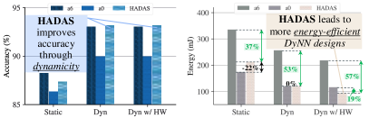
Figure 1: Comparing the performance of (a0, a6) from AttentiveNAS and HADAS’s model on CIFAR-100 and the Jetson TX2 Pascal GPU hardware

I-A Motivational Example

We take as baselines the respective most compact and highest-performing image recognition models, a0 and a6, that were provided through a state-of-the-art NAS framework, AttentiveNAS [5]. We compare their performance against one of our models that was provided using HADAS framework. In this case, we implement HADAS on top of AttentiveNAS to ensure a fair comparison by having the models share the same base structure and optimization algorithms. Classification accuracy and energy consumption are leveraged as the performance comparison metrics. Here, we use the CIFAR-100 image dataset for models’ training and accuracy evaluations and the NVIDIA Jetson TX2 platform for hardware benchmarking.

As shown in Figure 1, we designate three stages of optimizations that can be applied to maximize performance efficiency: Static – optimizing the backbone model design; Dyn – integrating dynamic early-exiting features; and Dyn w/ HW – integrating early-exiting features and applying DVFS features. With regards to accuracy (left barplot), HADAS’s model outperforms a0 and is on-par with a6 after applying the static and Dyn optimizations. More interestingly, though, the energy efficiency of HADAS’s model is enhanced considerably with every applied optimization compared to the other models (right barplot). After the first stage of Static optimization, a0 is reasonably deemed the most energy-efficient model given its compactness (22% more energy-efficient than ours). However, when Dyn optimizations are applied, our model’s efficiency improves drastically to reach the same level of energy efficiency as a0. Even more so, our model becomes 19% more energy-efficient than a0 once Dyn w/ HW optimizations are in place.

Analysis Summary and Conclusions: Through its awareness of the dynamic and DVFS parameter spaces, HADAS can balance the accuracy-efficiency trade-offs more than the conventional NN design approaches. Specifically, HADAS’s joint optimization approach of the backbone model, early exiting features, and the hardware settings leads to DyNN model designs that are highly prone to benefit from the static, dynamic, and hardware deployment aspects altogether.

I-B Novel Contributions

Our scientific contributions and novelties are as follows:

1. We present HADAS, a novel hardware-aware NAS framework that jointly optimizes the design of multi-exit DyNNs and DVFS settings for efficient edge operation.

2. As shown in Figure 2, HADAS is built to leverage the existing infrastructure of pretrained supernets provided through state-of-the-art NAS frameworks, and is also compatible with existing runtime controllers for an effective end-to-end design workflow.

3. We formulate the design space exploration problem for multi-exit architectures as a bi-level optimization problem solved through two nested evolutionary genetic engines. The outer engine identifies optimal backbone designs. Whereas the inner engine co-optimizes the exits’ integration and the DVFS settings.

4. On the CIFAR-100 dataset and a diverse set of hardware devices/settings, our experiments demonstrated that HADAS models can realize energy efficiency gains by up to $\sim$57% over models designed through conventional methods while preserving the desired level of accuracy.

II Related Works

Early exiting and NAS: Early-exiting has been widely adopted to realize DyNNs on the edge given their “simple-yet-effective” characteristic. The direct approach to realize Multi-exit networks has been to branch intermediate classifiers from the earlier stages of a backbone model, and retraining the model to maximize the performance of all classifiers [4, 2, 7, 8]. With an effective input-to-exit mapping policy, Multi-exit models enjoy computational efficiency as simpler input samples can be classified at the earlier classifiers (exits) while maintaining the model’s representational power through retaining the full classifier for the harder samples. In the aforementioned works, the multi-exit networks have been manually designed based on heuristic choices of positions, structure, and count conditioned on their respective backbone architecture [9]. Recent works [3, 10] have investigated the applicability of NAS techniques to automate the design of multi-exit networks, where the backbone and exits’ design spaces can be jointly explored to reach superior DyNN architectures. However, [3] instituted a small search space of one exit branch at a fixed position which is not scalable. Whereas despite the effectiveness of the approach in [10], its application was specific to convolutional NNs.

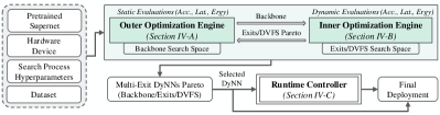
Figure 2: Overview of our Hardware-Aware Dynamic Neural Architecture Search (HADAS) framework. Lightly-shaded green blocks are the novel contributions.

Dynamic hardware reconfiguration: Dynamically scaling NNs results in different computational and energy footprints that require adapting the hardware configuration accordingly. In [11, 12], the hardware has been co-designed with the multi-exit networks using FPGAs, showcasing how further energy efficiency gains can be achieved through having specialized hardware for exits. Nevertheless, the considerable switching overheads of hardware configurations in FPGAs are not typically acceptable for runtime applications. A viable alternative came in the form of hardware reconfiguration through supported DVFS features, where the operational frequency can be scaled after exiting to preserve energy resources [13, 14]. Table I illustrates the difference between HADAS and existing multi-exit network design approaches and how it improves upon them through its joint optimization approach while being compatible with existing state-of-the-art NAS frameworks.

TABLE I: Comparison between Related-works and ours

Work	Early-Exiting	NAS	DVFS	Compatibility
BranchyNet [2]	x
CDLN [4]	x
S2dnas [10]	x	x
Dynamic-OFA [6]		x		x
EExNAS [3]	x	x
Edgebert [13]	x		x
Predictive Exit [14]	x		x
HADAS	x	x	x	x

III Problem Formulation

As the combined design space size for the DyNNs and hardware configurations can be enormous, we characterize three separate subspaces to manage the joint optimization of their parameters as follows: (i) The backbones ($\mathcal{B}$); which are models originally designed in a monolithic fashion for static inference with no adaptive behavior, (ii) The exits ($\mathcal{X}$); which are the dynamic components to be integrated onto a backbone, and (iii) The DVFS settings ($\mathcal{F}$); constituting the space of operational frequencies for the underlying hardware components. For the DyNNs, our reasons for designating $\mathcal{B}$ and $\mathcal{X}$ as separate subspaces are twofold: (a) To maintain the generality of the approach by having the $\mathcal{X}$ subspace indifferent to the “type” of candidate backbones in $\mathcal{B}$, and (b) To leverage the existing infrastructure of pretrained supernets from established NAS frameworks (as in [5, 15]) so as to provide high-caliber backbone models for the $\mathcal{B}$ subspace.

In order to rank candidate dynamic architectural designs, we denote $\mathcal{S}$ and $\mathcal{D}$ as generic performance objectives under static and dynamic deployments, respectively. Mainly, $\mathcal{S}$ represents the backbone evaluations when designated as a fixed standalone model (e.g., baseline energy), whereas $\mathcal{D}$ is for the evaluations of its dynamic variant after integrating the exits (e.g., average energy when effective mapping of inputs to exits). Hence, this implies a bi-level optimization problem with the $\mathcal{B}$ as the outer-level subspace and ($\mathcal{X}$, $\mathcal{F}$) as the inner-level ones:

$$b^{*}=\operatorname*{arg\,max}_{b\in\mathcal{B}}\;\psi[\mathcal{S}(b),\mathcal{D}(x^{*},f^{*}\;|\;b)]$$ (1)

$$s.t.\ x^{*},f^{*}=\operatorname*{arg\,max}_{x\in\mathcal{X},f\in\mathcal{F}}\;\mathcal{D}(x,f\;|\;b)$$ (2)

where the global optimization objective to identify the ideal parameter combination ($b^{*}$, $x^{*}$, $f^{*}$) that maximizes a global function $\psi$ combining the performance objectives of $\mathcal{S}$ and $\mathcal{D}$. In practice, the underlying optimization objectives are conflicting by nature – e.g., the larger computationally expensive models enjoy higher accuracy scores and vice versa. Thus, the problem can be approached as a multi-objective optimization where we seek a Pareto optimal set of solutions For instance, in equation (2), a solution ($x^{*}$, $f^{*}$) is said to be Pareto optimal if for all the objective functions $d$ $\in$ $\mathcal{D}$:

$$d_{k}(x^{*},f^{*})\geq d_{k}(x,f)\forall k,(x,f)\$$

$$\text{and}\ \exists j:d_{j}(x^{*},f^{*})>d_{j}(x,f)\forall(x,f)\neq(x^{*},f^{*})$$

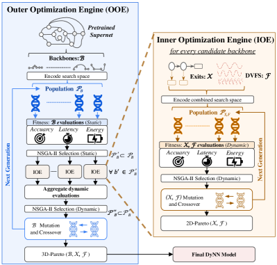
Figure 3: HADAS co-optimization framework.

IV Hadas Framework

We adopt nested genetic algorithms [16] to solve the optimization problem as illustrated in Figure 3 as follows:

IV-A Outer Optimization Engine (OOE)

The OOE considers two primary tasks: (i) Searching through $\mathcal{B}$ to identify the best backbone candidates, and (ii) Ranking DyNNs according to their aggregate $\mathcal{S}$ and $\mathcal{D}$ evaluations.

IV-A1 $\mathcal{B}$ Subspace

Modern NAS frameworks employ a Once-For-All (OFA) approach which entails first training a large over-parameterized supernet on a target task, prior to applying a search algorithm to identify the optimal subnet designs within. The enabling factor of OFA approaches is that all of the supernet’s parameters are shared by its subnets, effectively rendering the training and search procedures as disjoint processes, which dramatically reduces the overall overheads within the NAS framework [15, 5]. From here, HADAS is built to leverage the pretrained supernets of existing NAS frameworks to construct the $\mathcal{B}$ subspace of backbones, where the search space can be encoded into discrete variables usable by the search algorithm, and each viable subnet (backbone) can be denoted as $b\in\mathcal{B}$.

IV-A2 $\mathcal{B}$ Evolutionary Search

With $\mathcal{B}$ defined, the dynamic architecture search initiates in the OOE through an evolutionary search algorithm (e.g., NSGA-II) that can navigate through $\mathcal{B}$ to sample promising backbone models. In particular, the evolutionary algorithm is set to run for a predefined number of generations $G$, generating with every generation, $g$, a population of backbones, $\mathcal{P}_{\mathcal{B}}^{g}$, from which the encoded pretrained subnets can be sampled. Afterwards, $\forall b\in{P}_{\mathcal{B}}^{g}$, a fitness evaluation under static conditions is performed as:

$$\mathcal{S}(b)=Fit(Acc_{b},L_{b},E_{b})$$ (3)

where $\mathcal{S}(b)$ is a vector of the static performance evaluations with regards to the accuracy ($Acc_{b}$), latency ($L_{b}$), and energy ($E_{b}$), respectively. Estimates for $L_{b}$ and $E_{b}$ are obtained based on hardware measurements – as through a HW-in-the-loop setup (adopted here), lookup tables, or prediction models. At this stage, we remark that hardware evaluations are based on default HW settings, leaving the DVFS optimizations for the IOE. Based on the $\mathcal{S}$ scores, every $b\in{P}_{\mathcal{B}}^{g}$ is ranked using the NSGA-II non-dominated sorting algorithm. If a number of backbones shared the same rank, their diversity scores are used for re-ranking. This early selection procedure enables pruning the population to reach a smaller subset $\mathcal{P}_{\mathcal{B}}^{g^{\prime}}$ $\subset$ $\mathcal{P}_{\mathcal{B}}^{g}$, where every $b^{\prime}\in{P}_{\mathcal{B}}^{g^{\prime}}$ is mapped to an IOE (detailed later) to obtain the overall dynamic architecture evaluations $\mathcal{D}(x^{*},f^{*}\;|\;b^{\prime})$.

Once an IOE concludes its procedures, a Pareto optimal set of exits placement and DVFS settings is returned to the OOE for every $b^{\prime}\in{P}_{\mathcal{B}}^{g^{\prime}}$. These Pareto sets are then collectively aggregated for a second selection algorithm that ranks backbones based on their combined $\mathcal{S}$ and $\mathcal{D}$ scores, leading to another population subset $\mathcal{P}_{\mathcal{B}}^{g^{\prime\prime}}\subset\mathcal{P}_{\mathcal{B}}^{g^{\prime}}$. Lastly, $\mathcal{P}_{\mathcal{B}}^{g^{\prime\prime}}$ undergoes mutation and crossover operations to construct a new population $\mathcal{P}_{\mathcal{B}}^{g+1}$ for generation $g$+1. This outer loop cycle repeats until generation $G$ at which the Pareto optimal set ($b^{*}$, $x^{*}$, $f^{*}$) is returned as the final solution.

IV-B Inner Optimization Engine (IOE)

The IOE is invoked for every $b^{\prime}\in\mathcal{P}_{\mathcal{B}}^{g^{\prime}}$. Its primary responsibility is to search through the defined $\mathcal{X}$ and $\mathcal{F}$ subspaces to identify optimal pairings ($x^{*}$, $f^{*}\;|\;b^{\prime}$) as follows:

IV-B1 $\mathcal{X}$ subspace

To define the exits’ search space, we characterize the total number of exits and their positions as search parameters. In practice, present-day backbone structures (as those from AttentiveNAS) constitute $M$ sequential computing neural blocks (i.e., an aggregation of interrelated layers) between which effective placement of the exits can be realized. We illustrate this in Figure 4 through how the $\mathcal{X}$ subspace is conditioned on a $b\in\mathcal{B}$. Specifically, we define a vector of indicators $[\mathcal{I}_{1},\mathcal{I}_{2},...,\mathcal{I}_{M-1}]$ where $\mathcal{I}_{i}\in\{0,1\}$ to indicate whether exit branch at position $i$ is sampled for the corresponding instance. Regarding the composition of exit branches, we fix a simple structure across all potential exits positions for three reasons: (i) Re-usability as such a straightforward structure can act as a base module compatible with numerous backbone model architectures and classes, (ii) The smaller search space size of the exits leads to smaller search overheads – especially relevant when considering the additional subspaces as well, and (iii) Minimizing the training costs of the exits. For our experiments, the exit structure constituted a single sequential computing block of a convolutional, batch normalization and activation layers, which are followed by a final classifier layer.

IV-B2 Exits Training

Once a $b^{\prime}$ is mapped to the IOE, every $x\in\mathcal{X}$ needs to be trained for a fair evaluation of the exit candidates. In this scheme, the weight parameters of $b^{\prime}$ are kept frozen independent of the exits’ training procedure, where the rationale here is to avoid negatively influencing the performance of $b^{\prime}$ with regards to its static accuracy score (i.e., the backbone accuracy) – which can occur when the weights are optimized for more than one objective [2]. Combining this notion with the compact structure of the exits, the exits’ training overheads can be kept to a minimum within the IOE, all while leveraging the representational power of $b^{\prime}$ across its various stages to attain the desired resource efficiency gains.

For the training loss function itself, we adopt a hybrid loss function ($\mathcal{L}_{total}$) combining the Negative log-likelihood ($\mathcal{L}_{NLL}$) and knowledge distillation ($\mathcal{L}_{KD}$) loss components to simultaneously train every $x\in\mathcal{X}$ as follows:

$$\mathcal{L}=\frac{1}{N}\sum_{n=1}^{N}[\frac{1}{M\text{-1}}\sum_{m=1}^{M-1}(\mathcal{L}_{NLL}(y_{n},\hat{y}_{m,n})+\mathcal{L}_{KD}(\hat{y}_{m,n},\hat{y}_{M,n})]$$ (4)

where $N$ is the total number of training samples and $M-1$ is the total possible number of exits. For the $\mathcal{L}_{NLL}$ term, it aggregates the losses from every exit at $m$ when comparing its predicted outputs, $\hat{y}_{m,n}$, against the ground truth labels, $y_{n}$, for every sample $n$. Whereas the $\mathcal{L}_{KD}$ term aggregates the losses from comparing the error between every $\hat{y}_{m,n}$ and that of the final model classifier, $\hat{y}_{M,n}$. Due to space limitations, we illustrate how these loss components are defined in Figure 4, and refer interested readers to [7] for more details.

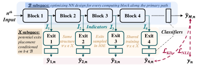
Figure 4: The combined $\mathcal{B}$ and $\mathcal{X}$ search spaces

IV-B3 $\mathcal{F}$ subspace

The hardware search space entails the DVFS configurations for enhancing the DyNN’s resource efficiency from the HW’s perspective. Given how different computational workloads utilize the underlying hardware components differently, DyNN design candidates can attain maximal resource efficiency at different DVFS settings. In practice, edge devices constitute heterogeneous computing units that support DVFS features. Thus, depending on the underlying hardware, the operational frequencies of CPU, GPU, and External Memory Controllers (EMC) can be used to construct $\mathcal{F}$.

IV-B4 ($\mathcal{X}$, $\mathcal{F}$) Evolutionary Search

Similar to the OOE, an IOE also operates an evolutionary NSGA-II algorithm to navigate the combined search spaces of $\mathcal{X}$ and $\mathcal{F}$. With each generation, a population $\mathcal{P}_{\mathcal{X},\mathcal{F}}$ is generated from the combined subspaces’ encoding and provided for the dynamic fitness evaluation:

$$\mathcal{D}(x,f\;|\;b^{\prime})=\frac{1}{\sum_{i=1}^{M\text{-1}}\mathcal{I}_{i}}\;\sum_{i=1}^{M\text{-1}}\;\mathcal{I}_{i}\cdot[score_{i}]$$ (5)

$$s.t.\;\;score_{i}=\mathcal{N}_{i}*\frac{E_{x_{i},f}}{E_{b}}*\frac{L_{x_{i},f}}{L_{b}}*(dissim_{i})^{\gamma}$$ (6)

where equation (5) reflects the mean dynamic performance score of a sampled dynamic model ($x$, $f\;|\;b^{\prime}$) through averaging scores for every sampled exit (recall $\mathcal{I}_{i}\in\{0,1\}$). An exit’s score is given by $score_{i}$ in equation 6, which constitutes: $\mathcal{N}_{i}$, the fraction of samples that can be correctly classified at exit $i$; $\frac{E_{x_{i},f}}{E_{b}}$, as the normalized dynamic energy at exit $x_{i}$ and DVFS settings $f$ relative to the backbone energy consumption; $\frac{L_{x_{i},f}}{L_{b}}$ is similarly the normalized dynamic latency term. $(dissim_{i})^{\gamma}$ is a regularization term with a trade-off parameter $\gamma$ measuring the dissimilarity of exit $x_{i}$ and its preceding ones as:

$$dissim_{i}=1-\max\;(\mathcal{N}_{0:i-1})$$ (7)

where $x_{i}$’s score is regularized in proportion to the fraction of samples that can be already classified by its preceding exits. The rationale behind this metric is to: (i) avoid sampling exits of similar performance characterizations, and (ii) realize a compact decision space for the DyNN when deployed.

Based on the $\mathcal{D}$ scores, every $(x,f\;|\;b^{\prime})\in{P}_{\mathcal{X},\mathcal{F}}$ is also ranked using the NSGA-II non-dominated sorting algorithm so as to realize subset ${P}_{\mathcal{X},\mathcal{F}}^{\prime}\subset{P}_{\mathcal{X},\mathcal{F}}$ that would then undergo mutation and crossover for the following generation. This loop cycle continues until the final generation where a 2-D Pareto optimal set ($x^{*}$, $f^{*}\;|\;b^{\prime}$) is returned to resume the OOE.

IV-C Runtime Controller

When a DyNN design is chosen for the final deployment, a runtime controller needs to be implemented to provide the effective input-to-exit mapping policies needed for dynamic inference. Concerning HADAS, its architectural optimizations are applied at the design stage of DyNNs under ideal mapping policies, that is, when every input is mapped to the first exit module $x_{i}$ that can classify it correctly. This is evident through how the score of each exit in eq. (6) is scaled based on $\mathcal{N}_{i}$ – the true fraction of correctly classified samples. Thus, models from HADAS are compatible with any class of runtime controllers existing in the literature (e.g., entropy-based [4, 2, 1]).

V Experiments and Results

V-A Experimental Setup

We implement HADAS on top of the AttentiveNAS framework [5]. To construct $\mathcal{B}$, we reuse their search space which contains more than $2.94\times 10^{11}$ neural networks generated by scaling different dimensions as stated in Table II. Our experiments are conducted on the CIFAR-100 dataset where the pretrained supernet of AttentiveNAS has been fine-tuned accordingly. Backbones and baselines are all sampled from the same fine-tuned supernet. We dynamically generate the exits’ search space $\mathcal{X}$ according to the supported depth $(l)$ of the backbones in $\mathcal{B}$. In our case, potential exit positions occur at a layer-wise granularity starting from the fifth (5) layer to the backbones’ last layer (For AttentiveNAS [5], potential exit positions are set after their “MBConv” layers). We evaluate our approach on 4 different hardware combinations from NVIDIA Edge devices: a) AGX Volta GPU, b) Carmel ARM v8.2 CPU, c) TX2 Pascal GPU, and d) NVIDIA Denver CPU. For each hardware setting, we leverage the supported DVFS configuration settings to generate $\mathcal{F}$ as in Table II. Regarding the optimization process, we fix a budget of 450 iterations for the OOE and 3500 iterations for the IOE, where #iterations = $\mathcal{G}$ $\times$ $\mathcal{P}$. We use a cluster of 32 GPUs to train the exits for every sampled backbone, taking up to $\sim$ 8-10 GPU hours for each $\mathcal{G}$. In our experiments, we used a HW-in-the-loop setup for latency and energy measurements which pushed the overall search time of HADAS to $\sim$2-3 GPU days. Nevertheless, based on our analysis, HADAS’s search overhead can be reduced to 1 GPU day if a proxy model replaced the HW-in-the-loop setup.

TABLE II: Details on HADAS joint search spaces in our experiments

Decision variables	Values	Cardinality
Backbone Search Space ($\mathcal{B}$)
Number of blocks (n_block)	7	1
Input resolution (res)	{192, 224, 256, 288}	4
Block depth (l)	{1, 2, 3, 4, 5, 6, 7, 8}	8
Block width (w)	[16, 1984]	16
Block kernel size (k)	{3, 5}	2
Block expand ratio (er)	{1, 4, 5, 6}	4
Exits Search Space ($\mathcal{X}$)
Number of exits (nX)	[1, ($\sum_{i=1}^{nb}l_{i})-5$]	max(nX)
Exit positions (posX)	[5, $\sum_{i=1}^{nb}l_{i})$]	$\binom{nx}{\sum_{i=1}^{nb}l_{i})}$
DVFS Search Space ($\mathcal{F}$)
GPU frequency (AGX Volta GPU)	[0.1GHz, 1.4GHz]	14
CPU frequency (Carmel ARM v8.2 CPU)	[0.1GHz, 2.3GHz]	29
GPU frequency (TX2 Pascal GPU)	[0.1GHz, 1.4GHz]	13
CPU frequency (NVIDIA Denver CPU)	[0.3GHz, 2.1GHz]	12
EMC frequency (AGX SOC)	[0.2GHz, 2.1GHz]	9
EMC frequency (TX2 SOC)	[0.2GHz, 1.8GHz]	11

V-B Co-optimization Results

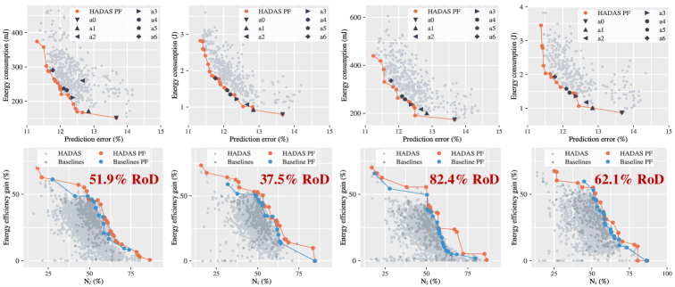
Figure 5: The top row gives the results of the outer optimization on 4 hardware settings of (from left to right): a) AGX Volta GPU, b) Carmel ARM v8.2 CPU, c) TX2 Pascal GPU, and d) NVIDIA Denver CPU. The bottom row shows the results of the inner optimization engine, with the same hardware settings. The points in the top row depict the static performance of the explored backbone neural networks in $(\mathcal{B})$ by the OOE, without early-exit or DVFS. The points in the bottom row represent the performance of the explored combinations of backbones, early-exits, and DVFS in $(\mathcal{B},\mathcal{X},\mathcal{F})$ by the IOE.

OOE Analysis: The top row of Figure 5 compares the static performance results from the OOE of HADAS against those of the top models from AttentiveNAS [5] (denoted as [a0-a6]). As shown, our obtained Pareto fronts (PF) generally dominate the baselines on the four hardware settings. Furthermore, HADAS can identify comparable backbones to the baselines with just a few evaluations. For instance, on the AGX Volta GPU, a6 is dominated by another backbone from HADAS with an energy reduction of $\sim 33\%$ under the same accuracy level. Similarly, a1 is dominated by another backbone from HADAS with an accuracy improvement of 2.34% under the same energy gain.

IOE Analysis: The results of the IOE are shown in the bottom row of Figure 5. For a fair comparison, we fix the same optimization budget when running the IOE for the baselines and HADAS. The dynamic performance of the explored $(b,x,f)$ combinations and the obtained Pareto fronts are given for both approaches, where the dynamic comparison metrics are the energy efficiency gains when early exiting and DVFS are supported, as well as the average of $N_{i}$ values from equation (6). Across the four hardware settings, HADAS seemingly dominates the majority of the optimized baselines with an average ratio of dominance 58.4% (detailed in the following paragraph). This can be attributed to HADAS’s better understanding of the global search space, where it samples backbones that are more poised to benefit from the IOE optimizations with regard to early exiting and DVFS. This is also evident through how HADAS can sample dynamic parameters for its models that can realize substantial energy or accuracy gains near the extremes of its Pareto frontier, which are not realizable by the optimized baselines. For instance on the Caramel ARM v8.2 CPU, energy gains reach 63% for one of the extreme dynamic models on the Pareto frontier of HADAS, compared to 52% for the extreme dynamic variant from the optimized baselines, under the same level of accuracy.

Hypervolume (HV) and Ratio of Dominance (RoD): we expand further on the IOE analysis and leverage hypervolume (HV) and ratio of dominance (RoD) as comparative evaluation metrics. The former metric measures the volume of the dominated portion of the objective space, whereas the latter measures the percentage of solutions found by HADAS that dominate the optimized baselines (and vice-versa). Figure 6 shows that HADAS consistently outperforms the optimized baselines with regards to both metrics across the 4 hardware platforms. Taking the Pascal GPU as an example, we find that the HV coverage and RoD are 16% and 95% more for HADAS over the optimized baselines, respectively.

TABLE III: DyNNs Comparison using the TX2 Pascal GPU

Model	Baseline Acc(%)	EEx Acc(%)	Baseline Ergy(mJ)	EEx Ergy(mJ)	EEx_DVFS Ergy(mJ)
AttentiveNAS_a0	86.33	89.95	173.78	119.83	116.14
AttentiveNAS_a6	88.23	93.02	335.48	256.80	218.34
HADAS_b1	87.34	93.16	212.44	119.84	93.78
HADAS_b2	88.06	91.83	341.3	187.92	126.06
HADAS_b3	86.54	88.31	205.48	130.20	86.84
HADAS_b4	88.40	89.24	358.01	232.77	201.01

DyNNs comparison: In Table III, we compare the top DyNNs obtained by HADAS with two AttentiveNAS models: a0, the most energy-efficient baseline, and a6, the most accurate baseline. Models are compared with regards to their static (i.e., baseline accuracy and energy) and their dynamic performances (i.e., accuracy and energy with early exiting and DVFS). As shown, the optimal models from HADAS outperform the baselines of AttentiveNAS in both static and dynamic evaluations. For instance, b1 from HADAS is 57% and 19% more energy-efficient than the a6 and a0, respectively, while enjoying similar accuracy scores like the most accurate model a6.

V-C Dissimilarity Ablation Study

We perform an ablation study to investigate the impact of the dissimilarity term ($dissim^{\gamma}$) in equation (6) through the performance of the explored models under each case. Specifically, we run the IOE for one backbone twice, with $dissim^{\gamma}$ not included and one when it is included. In Figure 7, we compare the results obtained with and without the dissimilarity with different values of $\gamma$. As shown, the inclusion of the dissimilarity term allows the optimization algorithm to focus more on exploring dissimilar early exits with a high contribution to the prediction accuracy. For instance, in the right of Figure 7, we find that the inclusion of dissimilarity improves RoD by 41%. Moreover, the extreme Pareto models with dissimilarity are $\sim$ 43% and $\sim$ 52% more accurate and energy efficient than those without dissimilarity.

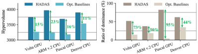
Figure 6: Comparing search efficacy for HADAS and the optimized baselines with regards to: a) hypervolume (left) and b) ratio of dominance (right)

VI Conclusion

We have presented HADAS, a novel HW-aware NAS framework that jointly optimizes the backbone, early exiting features, and DVFS for DyNNs. Through HADAS, large agile models can be realized with similar energy efficiency to that of compact models. We have shown that HADAS DyNNs can achieve up to 57% energy gains while retaining desired accuracy levels.

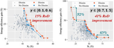
Figure 7: Inner optimization improvement by regularizing the exits scores with the dissimilarity function $(dissim)^{\gamma}$ over two ranges of $\gamma$ values

References

- [1] Y. Han et al., “Dynamic neural networks: A survey,” IEEE Transactions on Pattern Analysis and Machine Intelligence, 2021.
- [2] S. Teerapittayanon et al., “Branchynet: Fast inference via early exiting from deep neural networks,” in ICPR’16, 2016, pp. 2464–2469.
- [3] M. Odema et al., “EExNAS: Early-exit neural architecture search solutions for low-power wearable devices,” in 2021 IEEE/ACM International Symposium on Low Power Electronics and Design (ISLPED), 2021.
- [4] P. Panda, A. Sengupta, and K. Roy, “Conditional deep learning for energy-efficient and enhanced pattern recognition,” in 2016 Design, Automation & Test in Europe Conference & Exhibition (DATE), pp. 475–480.
- [5] D. Wang et al., “Attentivenas: Improving neural architecture search via attentive sampling,” in CVPR’21, 2021, pp. 6418–6427.
- [6] W. Lou et al., “Dynamic-ofa: Runtime dnn architecture switching for performance scaling on heterogeneous embedded platforms,” in Conference on Computer Vision and Pattern Recognition, 2021.
- [7] M. Phuong et al., “Distillation-based training for multi-exit architectures,” in Proc. of the IEEE/CVF Intl. Conf. on Computer Vision (ICCV), 2019.
- [8] G. Huang et al., “Multi-scale dense networks for resource efficient image classification,” arXiv preprint, 2017.
- [9] S. Laskaridis et al., “HAPI: Hardware-aware progressive inference,” in 2020 IEEE/ACM Intl. Conf. On Computer Aided Design (ICCAD), 2020.
- [10] Z. Yuan and al., “S2dnas: Transforming static cnn model for dynamic inference via neural architecture search,” in ECCV’20, 2020.
- [11] D. Paul, J. Singh, and J. Mathew, “Hardware-software co-design approach for deep learning inference,” in 2019 7th International Conference on Smart Computing & Communications (ICSCC). IEEE, 2019, pp. 1–5.
- [12] M. Farhadi et al., “A novel design of adaptive and hierarchical convolutional neural networks using partial reconfiguration on fpga,” in 2019 IEEE High Performance Extreme Computing Conference (HPEC), 2019.
- [13] T. Tambe and Al., “Edgebert: Sentence-level energy optimizations for latency-aware multi-task nlp inference,” in Micro-54, 2021, pp. 830–844.
- [14] X. Li et al., “Predictive exit: Prediction of fine-grained early exits for computation-and energy-efficient inference,” arXiv preprint, 2022.
- [15] H. Cai et al., “Once-for-all: Train one network and specialize it for efficient deployment,” arXiv preprint, 2019.
- [16] N. Fasfous et al., “AnaCoNGA: analytical HW-CNN co-design using nested genetic algorithms,” in 2022 Design, Automation & Test in Europe Conference & Exhibition (DATE). IEEE, 2022, pp. 238–243.