Switching to Discriminative Image Captioning
by Relieving a Bottleneck of Reinforcement Learning

Abstract

Discriminativeness is a desirable feature of image captions: captions should describe the characteristic details of input images. However, recent high-performing captioning models, which are trained with reinforcement learning (RL), tend to generate overly generic captions despite their high performance in various other criteria. First, we investigate the cause of the unexpectedly low discriminativeness and show that RL has a deeply rooted side effect of limiting the output words to high-frequency words. The limited vocabulary is a severe bottleneck for discriminativeness as it is difficult for a model to describe the details beyond its vocabulary. Then, based on this identification of the bottleneck, we drastically recast discriminative image captioning as a much simpler task of encouraging low-frequency word generation. Hinted by long-tail classification and debiasing methods, we propose methods that easily switch off-the-shelf RL models to discriminativeness-aware models with only a single-epoch fine-tuning on the part of the parameters. Extensive experiments demonstrate that our methods significantly enhance the discriminativeness of off-the-shelf RL models and even outperform previous discriminativeness-aware methods with much smaller computational costs. Detailed analysis and human evaluation also verify that our methods boost the discriminativeness without sacrificing the overall quality of captions.

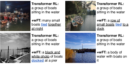
Figure 1: Caption examples in the MS COCO validation set. Transformer RL is a Transformer captioning model trained with RL and wFT is our fine-tuning method. Transformer RL generates exactly the same caption for the four images. The underlined words indicate the characteristic information that are not mentioned by Transformer RL, and the blue words are those that have never appeared in the outputs of the model. See Appendix 2 for more examples.

1 Introduction

Image captioning plays a fundamental role at the intersection of computer vision and natural language processing by converting the information in images into natural language descriptions. Generated captions can be used in various downstream tasks: aiding visually impaired users [19], visual question answering on images and videos [16, 31], visual dialogue [68], and news generation [79].

For those downstream tasks, captions should be discriminative: captions should describe the characteristic and important details of the input images [51]. However, current captioning models tend to generate overly generic captions [12, 11, 64, 66]. In particular, models trained with the standard reinforcement learning (RL) [50], which is the de facto standard training method in current image captioning [55], unexpectedly perform poorly in discriminativeness despite the significant advantages in various other criteria [39, 62]. For example, a high-performing Transformer [57] captioning model trained with RL generates exactly the same caption for the four different images shown in Figure 1, ignoring the other salient details of each image.

To address the problem of overly generic captions, studies have been intensely conducted on discriminative image captioning, which is also called distinctive image captioning or descriptive image captioning. Previous research has created new RL rewards regarding discriminativeness or new model architectures to enhance discriminativeness. These approaches improved the discriminativeness; however, their models come with additional computations, require retraining from scratch, and do not shed light on the cause of existing models’ low discriminativeness.

Instead of creating or paying those computational costs, we first analyze the cause of the unexpectedly low discriminativeness of off-the-shelf RL models, i.e., pre-trained, existing RL models, to explore ways to improve their discriminativeness. Our first contribution is the identification of a deeply rooted side effect in RL that limits output words to high-frequency words. The limited vocabulary is a severe bottleneck for discriminativeness as it is difficult for a model to describe the details beyond its vocabulary.

Given this identification of the bottleneck, now we can directly address the bottleneck by simply encouraging the generation of low-frequency words. This task relaxation allows us to introduce long-tail classification and debiasing methods to discriminative image captioning for the first time. Our second contribution is our effective and efficient methods that switch any off-the-shelf RL models to discriminativeness-aware models with only a single-epoch fine-tuning on the part of the parameters. Unlike previous approaches, our methods do not require any discriminativeness rewards, new model architectures, or retraining from scratch.

Extensive experiments demonstrate that increasing low-frequency words in outputs significantly boosts discriminativeness from off-the-shelf RL models and even outperforms previous discriminativeness-aware models with much smaller computational costs. These results verify that the limited vocabulary of RL models has been the major cause of their low discriminativeness. Detailed analysis and human evaluation also show that our methods enhance the discriminativeness without sacrificing the overall quality. We believe that our novel findings on the cause of low discriminativeness and the practical solutions to it will significantly impact future research on discriminative image captioning.

2 Discriminativeness and a Bottleneck of RL

Currently, RL is the de facto standard training method for models used in image captioning because it significantly improves the performance in various evaluation metrics [55]. However, it does not improve discriminativeness and may even decrease it [39, 62]. In this section, we examine the cause of the unexpectedly low discriminativeness.

2.1 RL in Image Captioning

We provide a brief overview of the standard RL algorithm used in image captioning. It was proposed by [48] and refined by [50]. Their goal was to directly optimize non-differentiable test-time metrics by minimizing the negative expected reward:

$$\mathcal{L}_{\mathrm{RL}}(\theta)=-\mathbb{E}_{w^{s}\sim p_{\theta}(w^{s}\mid I)}[r(w^{s})],$$ (1)

where $w^{s}=(w^{s}_{1},...,w^{s}_{T})$ is a sequence sampled from a policy $p_{\theta}$, $I$ is an input image, and $r(\cdot)$ is a reward function. To compute the gradient of $\mathcal{L}(\theta)$, [48] applied the REINFORCE algorithm [69] to text generation. The algorithm approximates the gradient as follows:

$$\nabla_{\theta}\mathcal{L}_{\mathrm{RL}}(\theta)\approx-(r(w^{s})-b)\nabla_{\theta}\log p_{\theta}(w^{s}\mid I).$$ (2)

Here, $b$ is a baseline reward that reduces the variance in the gradient. Typically, the reward function $r(\cdot)$ is CIDEr [59], and the baseline reward $b$ is a reward for a sequence sampled with greedy decoding [50].

Figure 2: Relative frequency of the words in the sequences sampled for the MS COCO training images. Five sequences were sampled for each image. The words (9,486 unique words excluding an out-of-vocabulary token $\langle\mathrm{unk}\rangle$) are sorted by their frequency in ground-truth captions and divided into 200 bins. We show the first 10 bins and the sum of the rest. GT is the ground-truth caption of the training images, CE is the output of a captioning model trained with the CE loss, and RL is the output of a captioning model trained with RL. Here, we used the Transformer model.

2.2 RL Limits Vocabulary

Despite its effectiveness, RL has been found not to improve discriminativeness and somehow decrease the number of unique n-grams in output captions [39, 62]. As the relation between RL and these two negative effects is not obvious, it has been just considered a curious case.

We elucidate for the first time the relation between RL and limited vocabulary by combining two recent findings. (1) RL has been shown to make the output distribution peaky [8, 30]. RL samples sequences from policy $p_{\theta}$ (See Eq. (1)). Typically, $p_{\theta}$ is initialized with a text-generation model pre-trained with the Cross-Entropy (CE) loss on ground-truth text. In text generation, however, the initialized $p_{\theta}$ outputs peaky distributions, and thus, RL samples and rewards the words at the peak only, shaping more peaky distributions [8]. Then, where does $p_{\theta}$ tend to be peaky? (2) Text-generation models have been theoretically and empirically shown to output distributions peaky at high-frequency words in the training corpus [46, 49, 13, 24]. These two findings conclude that RL shifts the probability mass from low-frequency words to high-frequency words by only sampling and rewarding the latter.

Figure 2 confirms the above by plotting the relative frequency of the words sampled for the training images. The words are sorted by their frequency in ground-truth captions and divided into 200 bins. Compared to the ground-truth captions and the sequences sampled with a CE model, the sequences sampled with an RL model are clearly limited to the high-frequency words, forming a peaky distribution.

2.3 Vocabulary Limits Discriminativeness

Neural captioning models typically generate captions using sequential vocabulary-size classification [61]. However, the actual vocabulary a model can generate is much smaller than the entire vocabulary as the output distribution is highly skewed towards high-frequency words. If the actual vocabulary cannot cover the details of an image, the model is forced to avoid those details and output only the information that high-frequency words can describe. For example, the blue words in Figure 1 are not in the actual vocabulary of the RL model; these words have never been generated during evaluation. As a result, the RL model had to ignore the characteristic relations tied and docked and ended up describing exactly the same for all four images.

Based on the observations, now we can hypothesize that the unexpectedly low discriminativeness of RL models has been rooted in the limited vocabulary. This identification of the bottleneck is a key contribution as it allows us to address the low discriminativeness directly at the root.

3 Methods to Relieve the Bottleneck

We have shown that RL results in the limited vocabulary as it steals the probability mass from low-frequency words. Thus, increasing those low-frequency words is the easy yet critical solution to the bottleneck. One way to achieve this is to jointly optimize both the RL loss and the CE loss on ground-truth captions so that the low-frequency words in ground-truth captions would be more likely to be sampled during RL training [64]. However, this approach still relies on the sampling from a skewed policy and requires retraining from scratch.

To increase the actual vocabulary more effectively and efficiently, we refine the mapping from encoded features to low-frequency words. This refinement can be applied to any RL models and can be achieved by modifying only the mapping function parameters with a single-epoch fine-tuning.

3.1 Simple Fine-Tuning (sFT)

The first method is a simple fine-tuning (sFT). It is based on a decoupled two-stage training [27], which is a current strong baseline model for long-tail classification [56, 44, 65]. [27] decoupled the learning procedure into representation learning and classification, and then found that classification, i.e., the mapping from representations to label distributions, is critical for long-tail classification. They decoupled the classification model $f_{\theta}(\cdot)$ into an encoder $g_{\theta_{e}}(\cdot)$ and a classifier consisting of weight and bias parameters: $f_{\theta}(x)=\bm{W}^{\top}g_{\theta_{e}}(x)+\bm{b}$. Representation learning is the first stage of training, where they trained the entire classification model $f_{\theta}(\cdot)$ on a full training dataset. The second stage is classification, where they fixed the encoder parameters $\theta_{e}$ and adjusted only the classifier parameters. For the second-stage adjustment, they applied class-balanced sampling to encourage learning on low-frequency labels.

Following [27], we decouple a captioning model into an encoder and a classifier. In image captioning, the first-stage training of [27] corresponds to RL training on the full training dataset. The second-stage training corresponds to adjusting the classifier parameters on the vocabulary-balanced sequences. However, sampling from the skewed policy of text-generation models cannot provide sequences containing low-frequency words (Section 2.2). Thus, we use ground-truth captions as relatively vocabulary-balanced samples. sFT simply fine-tunes the classifier parameters of a pre-trained RL captioning model by minimizing the CE loss on ground-truth captions:

$$\mathcal{L}_{\mathrm{CE}}(\hat{\theta})=-\frac{1}{T}\sum^{T}_{t=1}{\log p_{\hat{\theta}}(w^{g}_{t}\mid w^{g}_{<t},I)},$$ (3)

where $w^{g}=(w^{g}_{1},...,w^{g}_{T})$ is a ground-truth caption of image $I$ and $\hat{\theta}$ denotes the model parameters ${\theta}$ that are initialized with RL training. Let the softmax function $\phi(\cdot)$ be

$$\phi_{w_{i},\beta}(\bm{z})=\frac{\exp(\beta z_{w_{i}})}{\sum_{w_{j}\in\mathcal{W}}\exp(\beta z_{w_{j}})},$$ (4)

where $z_{w_{i}}$ indicates the element of a vector $\bm{z}\in\mathbb{R}^{|\mathcal{W}|}$ at the index of a word $w_{i}\in\mathcal{W}$. $\mathcal{W}$ is the entire vocabulary. $\beta$ is an inverse-temperature hyperparameter that controls the steepness of the softmax distribution. Then, the conditional probability $p_{\theta}(w^{g}_{t}\mid w^{g}_{<t},I)$ is computed as follows:

$$p_{\theta}(w^{g}_{t}\mid w^{g}_{<t},I) =\phi_{w^{g}_{t},\beta}(s^{t}_{\theta}(w^{g},I)),$$ (5)

$$s^{t}_{\theta}(w^{g},I) =\bm{W}^{\top}g_{\theta_{e}}(w^{g}_{<t},I)+\bm{b},$$ (6)

where $\bm{W}\in\mathbb{R}^{d\times|\mathcal{W}|}$ and $\bm{b}\in\mathbb{R}^{|\mathcal{W}|}$. $d$ is the dimension of the hidden states of an encoder $g_{\theta_{e}}(\cdot)$. We use LSTM [23] or Transformer [57] for $g_{\theta_{e}}(\cdot)$. During fine-tuning, only the classifier parameters $\{\bm{W},\bm{b}\}\in\hat{\theta}$ are updated with the gradients $\nabla_{\bm{W}}\mathcal{L}_{\mathrm{CE}}(\hat{\theta})$ and $\nabla_{\bm{b}}\mathcal{L}_{\mathrm{CE}}(\hat{\theta})$, respectively.

3.2 Weighted Fine-Tuning (wFT)

Ground-truth captions contain more low-frequency words than sampled sequences, but some low-frequency words are still difficult to learn because of their low frequency. Our second method is weighted fine-tuning (wFT), which further pursues vocabulary balance by rebalancing the loss of high-frequency words and low-frequency words in ground-truth captions.

To rebalance the loss, we exploit the frequency bias of RL models: RL models overly assign the probability to high-frequency words but not to low-frequency words. Given the properties of the frequency bias, fine-tuning for discriminativeness should focus more on the words that an RL model is not confident of but should be avoided on the words that an RL model is confident of. wFT incorporates these heuristics by modifying the probability $p_{\theta}$ of $\mathcal{L}_{\mathrm{CE}}$ to the bias product (BP) [9, 20, 22] probability, $p_{\theta,\theta^{\prime}}$:

$$p_{\theta,\theta^{\prime}}(w^{g}_{t}\mid w^{g}_{<t},I)=\\ \phi_{w^{g}_{t},1}\Big{[}\log\definecolor{tcbcolback}{rgb}{0.9,0.9,0.9}\definecolor{tcbcol@origin}{rgb}{0,0,0}\definecolor{.}{rgb}{0,0,0}\definecolor{.}{rgb}{0,0,0}\leavevmode\hbox to62.96pt{\vbox to35.94pt{\text{[drawing]}}}+\log\definecolor{tcbcolback}{rgb}{0.9,0.9,0.9}\definecolor{tcbcol@origin}{rgb}{0,0,0}\definecolor{.}{rgb}{0,0,0}\definecolor{.}{rgb}{0,0,0}\leavevmode\hbox to63.84pt{\vbox to36.38pt{\text{[drawing]}}}\Big{]}, p_{\theta}(\cdot\mid w^{g}_{<t},I) \phi_{\cdot,\beta}(s^{t}_{\theta}(w^{g},I)) p_{\theta^{\prime}}(\cdot\mid w^{g}_{<t},I) \phi_{\cdot,\beta^{\prime}}(s^{t}_{\theta^{\prime}}(w^{g},I)) p_{\theta}(\cdot\mid w^{g}_{<t},I) \phi_{\cdot,\beta}(s^{t}_{\theta}(w^{g},I)) p_{\theta^{\prime}}(\cdot\mid w^{g}_{<t},I) \phi_{\cdot,\beta^{\prime}}(s^{t}_{\theta^{\prime}}(w^{g},I))$$ (7)

where $\phi_{\cdot,\beta}(\bm{z})\in\mathbb{R}^{|\mathcal{W}|}$. By inserting $p_{\theta,\theta^{\prime}}$ into $\mathcal{L}_{\mathrm{CE}}$, we define the objective function of wFT as follows:

$$\mathcal{L}_{\mathrm{BP}}(\hat{\theta})=-\frac{1}{T}\sum^{T}_{t=1}{\log p_{\hat{\theta},\hat{\theta}^{\prime}}(w^{g}_{t}\mid w^{g}_{<t},I)}.$$ (8)

Similar to sFT, the parameters $\theta$ and $\theta^{\prime}$ are initialized with the same RL model to be $\hat{\theta}$ and $\hat{\theta}^{\prime}$. The difference is that, although the classifier parameters of $\hat{\theta}$ are updated, all the parameters of $\hat{\theta}^{\prime}$ are fixed during fine-tuning. Figure 3 shows the change in the BP loss compared to the CE loss. The BP severely suppresses the loss when the frequency-biased policy $p_{\theta^{\prime}}$ is confident, and largely increases the loss when $p_{\theta^{\prime}}$ is not confident. In this way, the BP allows models to unlearn the frequency bias learned with RL. As with sFT, only the classifier parameters $\{\bm{W},\bm{b}\}\in\hat{\theta}$ are updated with the gradients $\nabla_{\bm{W}}\mathcal{L}_{\mathrm{BP}}(\hat{\theta})$ and $\nabla_{\bm{b}}\mathcal{L}_{\mathrm{BP}}(\hat{\theta})$, respectively.

The previous BP methods used the probability $p_{\theta}$ during evaluation to avoid incorporating the bias of $p_{\theta^{\prime}}$ into the predictions [9, 20]. Although it worked well in their classification tasks, we found this train–test gap makes the decoding unstable in text generation. To mitigate the train–test gap, we use two variants of decoding: (1) decode with $p_{\theta}$ but use a small $\beta^{\prime}$ for $p_{\theta^{\prime}}$ during training to ease the gap between $p_{\theta}$ and $p_{\theta,\theta^{\prime}}$, or (2) use $p_{\theta,\theta^{\prime}}$ during both training and decoding (BP decoding) as $p_{\theta,\theta^{\prime}}$ itself is already less biased than $p_{\theta^{\prime}}$.

Figure 3: Visualization of the CE loss $-\log p_{\theta}(w_{i})$ and BP loss $-\log p_{\theta,\theta^{\prime}}(w_{i})$. To compute the BP loss, we need the entire distribution of $\{p_{\theta}(w_{i})\}_{w_{i}\in\mathcal{W}}$ and $\{p_{\theta^{\prime}}(w_{i})\}_{w_{i}\in\mathcal{W}}$. Here, we set the index $i$ to 1 and assigned $\frac{1}{5}(1-p_{\theta}(w_{1}))$ to the words of the next five indices, $w_{2},...,w_{6}$. This is because we observed that the five most probable words occupied 99% of the probability in the output distribution of the RL models. We assumed that the five most probable words were the same between $p_{\theta}$ and $p_{\theta^{\prime}}$ as the parameters were initialized with the same RL model. Thus, we assigned $\frac{1}{5}(1-p_{\theta^{\prime}}(w_{1}))$ to the words of the next five indices, $w_{2},...,w_{6}$, likewise $p_{\theta}$. Here, $\beta$ and $\beta^{\prime}$ were set to 1.

		Vocabulary			Standard Evaluation						Discriminativeness
		Unique-1	Unique-S	Length	CIDEr	SPICE	BERTS+	TIGEr	CLIPS	RefCLIPS	R@1	R@5	R@10
Att2in	Att2in RL	445	2,524	9.3	117.4	20.5	43.6	73.9	73.0	79.7	16.3	41.9	57.2
	+ sFT	880	3,156	9.0	115.4	20.4	43.9	74.3	73.7	80.3	20.1	48.0	62.8
	+ wFT	1,197	3,732	8.9	104.3	19.5	43.1	74.2	73.9	80.2	20.6	49.7	64.5
	+ wFT (BP decoding)	1,102	3,615	9.4	109.3	20.1	43.7	74.4	74.0	80.2	21.1	50.5	64.8
	CIDErBtw	470	2,630	9.3	119.0	20.7	43.8	74.1	73.1	79.8	17.2	44.1	58.7
	NLI	465	2,626	9.2	118.9	20.6	43.8	74.1	73.2	79.9	17.6	44.4	59.8
	DiscCap†		3,093	9.3	114.2	21.0					21.6	50.3	65.4
	Joint CE	700	2,907	9.1	111.7	19.9	43.5	74.0	73.3	80.0	19.1	46.7	61.5
	Only CE	689	2,845	9.2	110.7	20.1	43.5	74.0	73.3	79.9	19.0	46.6	61.1
1-14	Visual Paraphrase†		4,576	12.9	86.9	21.1					26.3	57.2	70.8
UpDown	UpDown RL	577	3,103	9.5	122.7	21.5	44.2	74.6	74.0	80.5	21.1	49.9	64.6
	+ sFT	1,190	3,788	9.2	115.9	21.0	44.2	74.9	74.8	80.9	25.0	56.8	71.2
	+ wFT	1,479	4,268	9.1	101.8	19.5	43.1	74.6	74.9	80.7	26.0	57.6	72.2
	+ wFT (BP decoding)	1,275	4,177	9.6	110.0	20.6	44.1	74.9	75.0	80.8	26.7	58.7	72.4
	CIDErBtw	582	3,108	9.4	123.0	21.5	44.4	74.6	74.2	80.7	21.9	50.9	65.9
	NLI	575	3,144	9.4	122.4	21.4	44.4	74.6	74.1	80.6	21.5	50.7	65.6
	Joint CE	857	3,120	9.4	111.8	20.5	43.7	74.3	73.8	80.2	21.8	51.2	65.2
	Only CE	878	3,126	9.4	109.2	20.1	43.4	74.2	73.6	80.0	21.8	49.9	64.5
Transformer	Transformer RL	753	3,433	9.2	127.7	22.5	45.1	75.0	75.0	81.3	26.6	56.2	70.5
	+ sFT	1,458	3,959	9.1	118.7	21.7	44.8	75.2	75.6	81.5	30.6	62.3	75.7
	+ wFT	1,776	4,274	9.1	103.1	20.0	43.3	74.8	75.8	81.2	32.5	64.5	77.1
	+ wFT (BP decoding)	1,964	4,373	9.4	107.3	21.1	44.2	75.2	76.1	81.5	33.5	65.9	78.2
	CIDErBtw	837	3,609	9.5	128.2	22.6	45.1	75.2	75.0	81.2	27.7	57.6	71.6
	NLI	876	3,744	9.5	129.1	23.0	45.4	75.3	75.5	81.5	29.8	59.9	73.4
	Joint CE	1,083	3,491	9.3	123.8	21.9	45.0	74.8	75.0	81.2	27.3	57.2	70.8
	Only CE	935	3,599	9.4	112.2	20.8	44.0	74.5	74.8	80.9	26.5	55.8	69.7

Table 1: Comparison of baseline models, our models, and state-of-the-art discriminativeness-aware models. Automatic evaluation results on the MS COCO test set. Unique-1 and Unique-S indicate the number of unique unigrams and sentences, respectively. Length is the average length of the output captions. Scores with ${{\dagger}}$ were reported in [39]. Other scores were reproduced by us.

4 Experiments

4.1 Setup

Dataset and Metrics. We used the MS COCO captioning dataset [38, 6] with Karpathy splitting [28]. After preprocessing, the entire vocabulary size $|\mathcal{W}|$ was 9,487. In the evaluation, the captions were decoded using a beam search of size 5 and evaluated using various evaluation metrics. Specifically, we used CIDEr [59] SPICE [1], Improved BERTScore (BERTS+) [74], TIGEr [25], CLIPScore (CLIPS), and RefCLIPScore (RefCLIPS) [21]. Note that the correlation with human judgments increases in the above order, with RefCLIPS indicating the state-of-the-art correlation [21, 29]. Following the previous studies [39, 62, 54], we evaluated discriminativeness with R@K scores: the percentage of captions with which a pre-trained image–text retrieval model [15] could correctly retrieve the original images from the entire validation/test images within the rank of K $\in\{1,5,10\}$. A higher R@K indicates that the model generates more discriminative captions with characteristic information of images. Evaluation was conducted in a single run for each model. See Appendix 4 for the libraries and settings we used for these evaluations.

Comparison Models. Following [62], we used Att2in [50], UpDown [2], and Transformer [57] as the baseline models. The models were pre-trained with the standard RL [50] and are publicly available. In addition to the baseline models, we compared our models with state-of-the-art discriminativeness-aware models: CIDErBtw [62], NLI [54], DiscCap [41], and Visual Paraphrase [39]. The first three created new discriminativeness rewards to be optimized with RL. Visual Paraphrase introduced a new model architecture to paraphrase simpler captions to more complex captions. See Section 5 for more details of these models. As we mentioned in the beginning of Section 3, the CE loss on ground-truth captions can be utilized in a different way from our methods. We report the results of jointly optimizing the RL loss and CE loss (Joint CE [64, 14]). It optimizes $\mathcal{L}_{\mathrm{Joint}}(\theta)=\lambda\mathcal{L}_{\mathrm{RL}}(\theta)+(1-\lambda)\mathcal{L}_{\mathrm{CE}}(\theta)$ during RL training. We also tested Only CE, which sets $\lambda=0$ to solely optimize the CE loss, as the baseline without RL. See Appendices 12 and 13 for more comparisons [76, 36, 7].

Hyperparameters. Our models used the same hyperparameters as the baseline models, except for the epoch size, learning rate, and $\beta^{\prime}$ in Eq. (7). We set the epoch size for fine-tuning to 1 and searched for the best learning rate from $\{1\textrm{e-}3,1\textrm{e-}4,1\textrm{e-}5,1\textrm{e-}6\}$. For BP in Eq. (7), we set $\beta=1$ and searched for the best $\beta^{\prime}$ from $\{0.1,1\}$. As with our models, we set all hyperparameters of the CE-based models to the same as the baseline models except for the $\lambda\in\{0,0.2,0.5,0.8\}$. We disabled scheduled sampling [4] for our fine-tuning and the CE loss to separate them from the RL loss strictly. We took the best hyperparameters according to the R@1 scores in the validation set. Note that we used different hyperparameters for the wFT with different decoding methods (See Section 3.2). Appendix 5 shows the best hyperparameters. We followed the previous work for the hyperparameters of the other models.

All the models except Visual Paraphrase had the same size of trainable parameters as their baselines. See Appendix 6 for the exact number of parameters. Our fine-tuning was completed in around 10 minutes using a single GPU of 16 GB memory. See Appendix 7 for the exact time for training and comparison with other methods.

4.2 Comparison with Baseline Models and Discriminativeness-Aware Models

Table 1 shows the results compared to those obtained with the baseline models and state-of-the-art discriminativeness-aware models.

Vocabulary. First, we observe that our methods (sFT and wFT) successfully increase the actual vocabulary size: both of them considerably increased Unique-1 compared to all the baseline models. wFT increased the vocabulary more than sFT, indicating that rebalancing the loss further encouraged low-frequency word generation. The increased vocabulary resulted in more specific captions to each image: Unique-S also increased significantly. Consistent with previous studies [64, 39, 62], the models trained with the CE loss (Joint CE and Only CE) achieved the larger vocabulary than the baseline RL models. However, the improvement of our methods was even larger than these CE-based models. Despite the significant increase in the vocabulary size, our method kept the captions concise: the average sentence length was close to those of the baseline models.

Discriminativeness. Our goal is to enhance the discriminativeness of RL models by addressing their limited vocabulary. As expected, our methods successfully improved the discriminativeness: the R@K scores of our models were considerably higher than those of the baselines. Corresponding to the better improvement in vocabulary size, wFT increased discriminativeness more than sFT. These results confirm our hypothesis that the limited vocabulary of RL models has been a major bottleneck for discriminativeness.

Among the Att2in-based models, Visual Paraphrase achieved the highest discriminativeness. However, this model is not directly comparable to the others because it increases the trainable parameters for its specialized model architecture. Moreover, its improvement in discriminativeness was achieved at the expense of conciseness, which is another desirable property for discriminative image captions [51]: its sentence length was substantially longer than the other models. DiscCap performed comparably with our models, but its reward requires high computational costs. CIDErBtw and NLI proposed more lightweight rewards to be applicable to larger models, but they still need retraining from scratch. Among the larger models (UpDown and Transformer), our models achieved the highest discriminativeness despite the small computational cost.

Standard Evaluation. As our methods increase low-frequency words in outputs, the outputs are likely to include the words that are out-of-references (OOR). That is, low-frequency words may not be covered by reference captions regardless of their correctness due to the low frequency. These low-frequency OOR words unfairly decrease scores in conventional evaluation metrics because those metrics count exact matches in the surface form of text.

To fairly evaluate the OOR words, recent metric research has focused on soft matching metrics [26, 21]. Soft-matching metrics can evaluate the semantic similarity between target captions and reference captions beyond the surface form of text by utilizing pre-trained language models (PLMs) [74, 77] or pre-trained cross-modal models (PCMs) [25, 33, 21]. Their correlation with human judgments is significantly higher than that of exact-matching metrics in both precision and recall [29]. In particular, PCM-based metrics, which can utilize image features in addition to reference captions, have substantially enhanced the evaluation performance and have achieved the state-of-the-art correlation with human judgments [21, 29].

Given the above advantages, we employed soft-matching metrics in addition to conventional exact-matching metrics. Not surprisingly, our models decreased the scores in the exact-matching metrics (CIDEr and SPICE). However, our models scored comparably with the baselines in the PLM-based metric (BERTS+) and rather outperformed them in the state-of-the-art PCM-based metrics (TIGEr, CLIPS, and RefCLIPS). The higher performance in the superior soft-matching metrics indicates that our methods do not degrade the overall quality of captions. To further validate the overall quality of our output captions, the following Section 4.3 analyzes the cause of this performance gap in more detail.

				Text-Based			Text-and-Image-Based
	Repetition	OOR		Exact-Matching		Soft-Matching
	Rep (%) $\downarrow$	Number $\downarrow$	Rank $\uparrow$	CIDEr	SPICE	BERTS+	TIGEr	CLIPS	RefCLIPS
Att2in RL	4.1	8,665	79.4	117.4	20.5	43.6	73.9	73.0	79.7
+ sFT	3.8	8,813	164.0	115.4	20.4	43.9	74.3	73.7	80.3
+ wFT	3.2	10.454	237.9	104.3	19.5	43.1	74.2	73.9	80.2
+ wFT (BP decoding)	3.6	10,386	204.7	109.3	20.1	43.7	74.4	74.0	80.2
Only CE	3.9	9,913	133.1	110.7	20.1	43.5	74.0	73.3	79.9
UpDown RL	3.9	8,463	100.1	122.7	21.5	44.2	74.6	74.0	80.5
+ sFT	3.6	9,252	225.8	115.9	21.0	44.2	74.9	74.8	80.9
+ wFT	3.0	11,478	301.0	101.8	19.5	43.1	74.6	74.9	80.7
+ wFT (BP decoding)	3.4	11,065	236.9	110.0	20.6	44.1	74.9	75.0	80.8
Only CE	3.7	10,874	152.9	109.2	20.1	43.4	74.2	73.6	80.0
Transformer RL	3.6	7,824	129.8	127.7	22.5	45.1	75.0	75.0	81.3
+ sFT	3.2	9,397	296.0	118.7	21.7	44.8	75.2	75.6	81.5
+ wFT	2.6	11,930	379.7	103.1	20.0	43.3	74.8	75.8	81.2
+ wFT (BP decoding)	2.9	11,673	461.0	107.3	21.1	44.2	75.2	76.1	81.5
Only CE	3.3	10,661	165.6	112.2	20.8	44.0	74.5	74.8	80.9
Human	2.4	17,963	815.6	88.4	21.2	42.9	73.3	77.7	82.0

Table 2: Comparison of OOR words and the resulting difference in exact-matching and soft-matching metrics. We report the results on the MS COCO test set. A higher value in Rank indicates a lower frequency rank of the OOR words. We also report the rate of repetition.

	Discriminativeness	Correctness	Fluency
Transformer RL	3.00	4.42	4.83
+ wFT	3.34∗∗	4.45	4.84
NLI	3.18∗∗	4.54	4.76

Table 3: Human evaluation results on the subset of the MS COCO test set. The discriminativeness score of Transformer RL was fixed at 3.00 because we set it as the baseline. ^∗/^∗∗ indicates that a score is statistically significantly different from that of the baseline model (t-test with $p<0.05/0.01$); one-sample t-test for discriminativeness and independent two-sample t-test for the other criteria.

4.3 Analysis of the Performance Gap

Properties of OOR Words. The critical difference between the conventional exact-matching metrics and the recent soft-matching metrics is the (in)ability to evaluate OOR words. Based on the difference, we hypothesize that the performance gap is caused by a difference in the properties of OOR words. We analyzed the OOR words of our models, comparing with those of RL baselines and Only CE, which scores similarly to our models in exact-matching metrics but decreases soft-matching scores in contrast to our models. Table 2 shows the number of OOR words and their average frequency rank. The frequency rank refers to the order of words when sorted by their frequency in training captions; the most frequent word ranks 1st, and the value of rank increases as the frequency decreases. Although our models and Only CE output the similar number of OOR words, the significant difference in the frequency rank indicates that the properties of our OOR words are different from those of Only CE; that is, the OOR words of our models consist of much more low-frequency words than those of Only CE. Low-frequency words are likely to be OOR by the nature of their frequency, regardless of their correctness.

The soft-matching metrics could tell this difference and scored our models higher than Only CE models and even higher than baseline RL models. Especially, this tendency was more clear in the state-of-the-art PCM-based metrics (TIGEr, CLIPS, and RefCLIPS). On the contrary, the exact-matching metrics (CIDEr and SPICE) could not tell the difference by definition and decreased the scores roughly in proportion to the number of OOR words. Appendix 8 shows the qualitative analysis of the underrated captions.

Comparison with Human-Annotated Captions. Human-annotated captions are known to show low exact-matching scores despite their high quality [29, 39, 11]. In Table 2, we observe that human-annotated captions (Human) have similar properties to ours: a large number of low-frequency OOR words, low exact-matching scores, but high scores in the state-of-the-art metrics (CLIPS and RefCLIPS).

Repetition. We also confirmed that the decrease in exact-matching scores was not caused by repetition, which is a typical side effect of heavily maximizing discriminativeness rewards [64, 60]. Table 2 shows that our models’ repetition rates were rather lower than those of baselines.

Conclusion. From the above results, we conclude that the lower exact-matching scores of our models are caused by the nature of low-frequency words and the deficiency of exact-matching metrics, not by the degeneration of our models. The results of the human evaluation in the following Section 4.4 further support this conclusion.

4.4 Human Evaluation

As discussed in Sections 4.2 and 4.3, automatic evaluation of our models has difficulty due to the OOR words caused by the low frequency. To further validate the performance of our models, we conducted human evaluations using Amazon Mechanical Turk (AMT) on three criteria: discriminativeness, correctness, and fluency. Correctness and fluency are absolute scores: we instructed workers to give a maximum score 5 to the captions that did not contain incorrect information (ungrammatical or unnatural expressions) in terms of correctness (fluency). In contrast, discriminativeness is designed as a relative score because it is difficult to set an absolute standard for discriminativeness; unlike correctness or fluency, we cannot define the perfectly discriminative captions. Following [62], we instructed the workers to determine the discriminativeness of a caption by comparing the caption with that of a baseline model.

We evaluated the Transformer-based models, which performed the best in the automatic evaluation. Although wFT with BP decoding performed better, here we picked up wFT with $p_{\theta}$ decoding to set the total number of parameters for decoding strictly the same across the models. Following [62], we randomly selected 50 images from the MS COCO test set and assigned five workers to each image. See Appendix 9 for more details on the AMT instruction. Table 3 shows the results. wFT, which had the highest R@K scores, also achieved the highest discriminativeness here. wFT achieved the same or higher correctness and fluency than the baseline model, in contrast to the exact-matching scores in Table 2. These results are consistent with the results of the state-of-the-art soft-matching metrics, confirming again that our methods do not degrade the quality of captions.

5 Related Work

Image Captioning is the task of describing images in natural languages. The quality of captions has been remarkably improved by recent advances such as the encoder–decoder captioning model [61], attention mechanism [73], RL training [48, 50], attention over bounding box features [2], large-scale pre-training [36], and large-scale captioning datasets [75, 38, 6, 32, 52]. Despite these advancements, current captioning models generate overly generic captions [12, 11, 64, 66].

Discriminative Image Captioning has been explored to generate more informative captions. [51] was the first to study it. They defined the more informative captions as the captions that concisely describe the information discriminative from distractor images, i.e., images similar to an input image. [3] proposed neural listener and speaker models that cooperate to generate discriminative captions for abstract scenes. [45] adapted the models to single-colored images. [58, 10] extended the domain to real images and improved inference efficiency. [63] proposed a memory attention network to describe unique objects among distractor images. [43] introduced a dataset with harder distractor images.

These approaches require selecting distractor images for inference. [41] and [40] proposed the methods that do not require this step. Their models learn to generate discriminative captions by maximizing the R@K scores for sampled captions using RL [50]. The R@K scores are computed with a pre-trained image–text retrieval model [15] over images in a mini-batch. [60] proposed a method to jointly train the image–text retrieval model and captioning model. Despite their effectiveness, R@K scores are associated with high computational costs and require a large batch size. Recently, CIDErBtw [62] and NLI [54] achieved state-of-the-art discriminativeness with more lightweight rewards. They weighted the contribution of ground-truth captions for the CIDEr reward according to their differences from similar but different captions [62] or their entailment scores against other ground-truth captions [54]. Another approach exploited unrelated captions as negative examples and trained caption generators with contrastive learning [12] or GAN [12, 17].

Visual Paraphrase [39] and [70] are related to our work in that they exploited low-frequency n-grams to enhance discriminativeness. [39] divided ground-truth captions into two subsets according to n-gram TF-IDF scores and proposed a new model to paraphrase low TF-IDF captions into high TF-IDF ones. [70] proposed the use of n-gram TF-IDF scores as an additional reward to a variant of R@K reward.

Different from above approaches, our objective is set to remedy the low discriminativeness of existing RL models. Our models can be achieved with single-epoch fine-tuning of pre-trained RL models, without requiring either drastic changes in the model architecture [39], additional computational costs of rewards [70], or retraining from scratch.

Diverse Image Captioning is the task of generating a set of diverse captions for a given image [67]. Diverse image captioning is aimed at enumerating various pieces of information with a set of captions, whereas discriminative image captioning aims to concisely describe the most characteristic information with a single caption. Similar to this study, some studies utilized captions that contained more low-frequency words, such as ground-truth captions [64, 42] or captions sampled from CE models [53]. Their models learn to generate these captions in addition to the captions sampled from RL models. However, these approaches still rely on sampling from skewed policies and require retraining of a model from scratch.

Long-Tail Classification has been studied extensively in various tasks as label imbalance is prevalent across datasets [78, 35]. In text-generation tasks, label imbalance exists in the frequency of words. Previous approaches have addressed the imbalance by normalizing classifier weights [46, 49] or using variants of Focal loss [49, 18, 26, 72, 37]. In contrast to these approaches, we adapted long-tail classification to mitigate the side effects of RL in the context of discriminative image captioning. Appendix 10 shows that our methods outperformed these approaches.

6 Conclusion

We have investigated the cause of overly generic captions of RL models and found out that RL decreases the discriminativeness by limiting the output words to high-frequency words. We propose the lightweight fine-tuning methods to address the bottleneck directly and achieve significantly higher discriminativeness with only the slight modification on off-the-shelf RL models. Our identification of the bottleneck and practical solutions will significantly impact future research on discriminative image captioning.

As an additional practical advantage, our models can control the granularity of descriptions from coarse to fine by just switching the off-the-shelf/fine-tuned classifier parameters. In terms of broader impact, our methods can be easily applied to the RL models in other text generation tasks, such as machine translation [71], summarization [47], and dialogue generation [34] to enrich the output vocabulary.

References

- [1] Peter Anderson, Basura Fernando, Mark Johnson, and Stephen Gould. Spice: Semantic propositional image caption evaluation. In ECCV, 2016.
- [2] Peter Anderson, Xiaodong He, Chris Buehler, Damien Teney, Mark Johnson, Stephen Gould, and Lei Zhang. Bottom-up and top-down attention for image captioning and visual question answering. In CVPR, 2018.
- [3] Jacob Andreas and Dan Klein. Reasoning about pragmatics with neural listeners and speakers. In EMNLP, 2016.
- [4] Samy Bengio, Oriol Vinyals, Navdeep Jaitly, and Noam Shazeer. Scheduled sampling for sequence prediction with recurrent neural networks. In NeurIPS, 2015.
- [5] Tianlang Chen, Zhongping Zhang, Quanzeng You, Chen Fang, Zhaowen Wang, Hailin Jin, and Jiebo Luo. “factual”or“emotional”: Stylized image captioning with adaptive learning and attention. In ECCV, 2018.
- [6] Xinlei Chen, Hao Fang, Tsung-Yi Lin, Ramakrishna Vedantam, Saurabh Gupta, Piotr Dollár, and C Lawrence Zitnick. Microsoft coco captions: Data collection and evaluation server. arXiv preprint arXiv:1504.00325, 2015.
- [7] Jaemin Cho, Seunghyun Yoon, Ajinkya Kale, Franck Dernoncourt, Trung Bui, and Mohit Bansal. Fine-grained image captioning with CLIP reward. In Findings of the Association for Computational Linguistics: NAACL 2022, 2022.
- [8] Leshem Choshen, Lior Fox, Zohar Aizenbud, and Omri Abend. On the weaknesses of reinforcement learning for neural machine translation. In ICLR, 2020.
- [9] Christopher Clark, Mark Yatskar, and Luke Zettlemoyer. Don’t take the easy way out: Ensemble based methods for avoiding known dataset biases. In EMNLP-IJCNLP, 2019.
- [10] Reuben Cohn-Gordon, Noah Goodman, and Christopher Potts. Pragmatically informative image captioning with character-level inference. In NAACL-HLT, 2018.
- [11] Bo Dai, Sanja Fidler, Raquel Urtasun, and Dahua Lin. Towards diverse and natural image descriptions via a conditional gan. In ICCV, 2017.
- [12] Bo Dai and Dahua Lin. Contrastive learning for image captioning. In NeurIPS, 2017.
- [13] David Demeter, Gregory Kimmel, and Doug Downey. Stolen probability: A structural weakness of neural language models. In ACL, 2020.
- [14] Sergey Edunov, Myle Ott, Michael Auli, David Grangier, and Marc’Aurelio Ranzato. Classical structured prediction losses for sequence to sequence learning. In NAACL-HLT, 2018.
- [15] Fartash Faghri, David J Fleet, Jamie Ryan Kiros, and Sanja Fidler. Vse++: Improving visual-semantic embeddings with hard negatives. In BMVC, 2018.
- [16] Adam Fisch, Kenton Lee, Ming-Wei Chang, Jonathan H Clark, and Regina Barzilay. Capwap: Captioning with a purpose. In EMNLP, 2020.
- [17] Ian Goodfellow, Jean Pouget-Abadie, Mehdi Mirza, Bing Xu, David Warde-Farley, Sherjil Ozair, Aaron Courville, and Yoshua Bengio. Generative adversarial nets. In NeurIPS, 2014.
- [18] Shuhao Gu, Jinchao Zhang, Fandong Meng, Yang Feng, Wanying Xie, Jie Zhou, and Dong Yu. Token-level adaptive training for neural machine translation. In EMNLP, 2020.
- [19] Danna Gurari, Yinan Zhao, Meng Zhang, and Nilavra Bhattacharya. Captioning images taken by people who are blind. In ECCV, 2020.
- [20] He He, Sheng Zha, and Haohan Wang. Unlearn dataset bias in natural language inference by fitting the residual. In EMNLP-IJCNLP, 2019.
- [21] Jack Hessel, Ari Holtzman, Maxwell Forbes, Ronan Le Bras, and Yejin Choi. Clipscore: A reference-free evaluation metric for image captioning. In EMNLP, 2021.
- [22] Geoffrey E Hinton. Training products of experts by minimizing contrastive divergence. Neural computation, 14(8):1771–1800, 2002.
- [23] Sepp Hochreiter and Jürgen Schmidhuber. Long short-term memory. Neural computation, 9(8):1735–1780, 1997.
- [24] Ari Holtzman, Jan Buys, Li Du, Maxwell Forbes, and Yejin Choi. The curious case of neural text degeneration. In ICLR, 2020.
- [25] Ming Jiang, Qiuyuan Huang, Lei Zhang, Xin Wang, Pengchuan Zhang, Zhe Gan, Jana Diesner, and Jianfeng Gao. Tiger: Text-to-image grounding for image caption evaluation. In EMNLP-IJCNLP, 2019.
- [26] Shaojie Jiang, Pengjie Ren, Christof Monz, and Maarten de Rijke. Improving neural response diversity with frequency-aware cross-entropy loss. In WWW, 2019.
- [27] Bingyi Kang, Saining Xie, Marcus Rohrbach, Zhicheng Yan, Albert Gordo, Jiashi Feng, and Yannis Kalantidis. Decoupling representation and classifier for long-tailed recognition. In ICLR, 2020.
- [28] Andrej Karpathy and Li Fei-Fei. Deep visual-semantic alignments for generating image descriptions. In CVPR, 2015.
- [29] Jungo Kasai, Keisuke Sakaguchi, Lavinia Dunagan, Jacob Morrison, Ronan Le Bras, Yejin Choi, and Noah A. Smith. Transparent human evaluation for image captioning. In NAACL-HLT, 2022.
- [30] Samuel Kiegeland and Julia Kreutzer. Revisiting the weaknesses of reinforcement learning for neural machine translation. In NAACL-HLT, 2021.
- [31] Hyounghun Kim, Zineng Tang, and Mohit Bansal. Dense-caption matching and frame-selection gating for temporal localization in videoqa. In ACL, 2020.
- [32] Ranjay Krishna, Yuke Zhu, Oliver Groth, Justin Johnson, Kenji Hata, Joshua Kravitz, Stephanie Chen, Yannis Kalantidis, Li-Jia Li, David A Shamma, Michael Bernstein, and Li Fei-Fei. Visual genome: Connecting language and vision using crowdsourced dense image annotations. IJCV, 123(1):32–73, 2017.
- [33] Hwanhee Lee, Seunghyun Yoon, Franck Dernoncourt, Doo Soon Kim, Trung Bui, and Kyomin Jung. ViLBERTScore: Evaluating image caption using vision-and-language BERT. In The First Workshop on Evaluation and Comparison of NLP Systems, 2020.
- [34] Jiwei Li, Will Monroe, Alan Ritter, Dan Jurafsky, Michel Galley, and Jianfeng Gao. Deep reinforcement learning for dialogue generation. In EMNLP, 2016.
- [35] Xiaoya Li, Xiaofei Sun, Yuxian Meng, Junjun Liang, Fei Wu, and Jiwei Li. Dice loss for data-imbalanced nlp tasks. In ACL, 2020.
- [36] Xiujun Li, Xi Yin, Chunyuan Li, Pengchuan Zhang, Xiaowei Hu, Lei Zhang, Lijuan Wang, Houdong Hu, Li Dong, Furu Wei, et al. Oscar: Object-semantics aligned pre-training for vision-language tasks. In ECCV, 2020.
- [37] Tsung-Yi Lin, Priya Goyal, Ross Girshick, Kaiming He, and Piotr Dollár. Focal loss for dense object detection. In ICCV, 2017.
- [38] Tsung-Yi Lin, Michael Maire, Serge Belongie, James Hays, Pietro Perona, Deva Ramanan, Piotr Dollár, and C Lawrence Zitnick. Microsoft coco: Common objects in context. In ECCV, 2014.
- [39] Lixin Liu, Jiajun Tang, Xiaojun Wan, and Zongming Guo. Generating diverse and descriptive image captions using visual paraphrases. In ICCV, 2019.
- [40] Xihui Liu, Hongsheng Li, Jing Shao, Dapeng Chen, and Xiaogang Wang. Show, tell and discriminate: Image captioning by self-retrieval with partially labeled data. In ECCV, 2018.
- [41] Ruotian Luo, Brian Price, Scott Cohen, and Gregory Shakhnarovich. Discriminability objective for training descriptive captions. In CVPR, 2018.
- [42] Ruotian Luo and Gregory Shakhnarovich. Analysis of diversity-accuracy tradeoff in image captioning. arXiv preprint arXiv:2002.11848, 2020.
- [43] Yangjun Mao, Long Chen, Zhihong Jiang, Dong Zhang, Zhimeng Zhang, Jian Shao, and Jun Xiao. Rethinking the reference-based distinctive image captioning. In ACM MM, 2022.
- [44] Aditya Krishna Menon, Sadeep Jayasumana, Ankit Singh Rawat, Himanshu Jain, Andreas Veit, and Sanjiv Kumar. Long-tail learning via logit adjustment. In ICLR, 2020.
- [45] Will Monroe, Robert XD Hawkins, Noah D Goodman, and Christopher Potts. Colors in context: A pragmatic neural model for grounded language understanding. TACL, 5:325–338, 2017.
- [46] Toan Q Nguyen and David Chiang. Improving lexical choice in neural machine translation. In NAACL-HLT, 2018.
- [47] Ramakanth Pasunuru and Mohit Bansal. Multi-reward reinforced summarization with saliency and entailment. In NAACL-HLT. ACL, 2018.
- [48] Marc’Aurelio Ranzato, Sumit Chopra, Michael Auli, and Wojciech Zaremba. Sequence level training with recurrent neural networks. In ICLR, 2015.
- [49] Vikas Raunak, Siddharth Dalmia, Vivek Gupta, and Florian Metze. On long-tailed phenomena in neural machine translation. In Findings of the Association for Computational Linguistics: EMNLP 2020, 2020.
- [50] Steven J Rennie, Etienne Marcheret, Youssef Mroueh, Jerret Ross, and Vaibhava Goel. Self-critical sequence training for image captioning. In CVPR, 2017.
- [51] Amir Sadovnik, Yi-I Chiu, Noah Snavely, Shimon Edelman, and Tsuhan Chen. Image description with a goal: Building efficient discriminating expressions for images. In CVPR, 2012.
- [52] Piyush Sharma, Nan Ding, Sebastian Goodman, and Radu Soricut. Conceptual captions: A cleaned, hypernymed, image alt-text dataset for automatic image captioning. In ACL, 2018.
- [53] Jiahe Shi, Yali Li, and Shengjin Wang. Partial off-policy learning: Balance accuracy and diversity for human-oriented image captioning. In ICCV, 2021.
- [54] Zhan Shi, Hui Liu, and Xiaodan Zhu. Enhancing descriptive image captioning with natural language inference. In ACL, 2021.
- [55] Matteo Stefanini, Marcella Cornia, Lorenzo Baraldi, Silvia Cascianelli, Giuseppe Fiameni, and Rita Cucchiara. From show to tell: A survey on image captioning. arXiv preprint arXiv:2107.06912, 2021.
- [56] Kaihua Tang, Jianqiang Huang, and Hanwang Zhang. Long-tailed classification by keeping the good and removing the bad momentum causal effect. In NeurIPS, 2020.
- [57] Ashish Vaswani, Noam Shazeer, Niki Parmar, Jakob Uszkoreit, Llion Jones, Aidan N Gomez, Łukasz Kaiser, and Illia Polosukhin. Attention is all you need. In NeurIPS, 2017.
- [58] Ramakrishna Vedantam, Samy Bengio, Kevin Murphy, Devi Parikh, and Gal Chechik. Context-aware captions from context-agnostic supervision. In CVPR, 2017.
- [59] Ramakrishna Vedantam, C Lawrence Zitnick, and Devi Parikh. Cider: Consensus-based image description evaluation. In CVPR, 2015.
- [60] Gilad Vered, Gal Oren, Yuval Atzmon, and Gal Chechik. Joint optimization for cooperative image captioning. In ICCV, 2019.
- [61] Oriol Vinyals, Alexander Toshev, Samy Bengio, and Dumitru Erhan. Show and tell: A neural image caption generator. In CVPR, 2015.
- [62] Jiuniu Wang, Wenjia Xu, Qingzhong Wang, and Antoni B Chan. Compare and reweight: Distinctive image captioning using similar images sets. In ECCV, 2020.
- [63] Jiuniu Wang, Wenjia Xu, Qingzhong Wang, and Antoni B Chan. Group-based distinctive image captioning with memory attention. In ACM MM, 2021.
- [64] Qingzhong Wang and Antoni B Chan. Describing like humans: on diversity in image captioning. In CVPR, 2019.
- [65] Xudong Wang, Long Lian, Zhongqi Miao, Ziwei Liu, and Stella Yu. Long-tailed recognition by routing diverse distribution-aware experts. In ICLR, 2020.
- [66] Zeyu Wang, Berthy Feng, Karthik Narasimhan, and Olga Russakovsky. Towards unique and informative captioning of images. In ECCV, 2020.
- [67] Zhuhao Wang, Fei Wu, Weiming Lu, Jun Xiao, Xi Li, Zitong Zhang, and Yueting Zhuang. Diverse image captioning via grouptalk. In IJCAI, 2016.
- [68] Julia White, Gabriel Poesia, Robert Hawkins, Dorsa Sadigh, and Noah Goodman. Open-domain clarification question generation without question examples. In EMNLP, 2021.
- [69] Ronald J Williams. Simple statistical gradient-following algorithms for connectionist reinforcement learning. Machine learning, 8(3):229–256, 1992.
- [70] Jie Wu, Tianshui Chen, Hefeng Wu, Zhi Yang, Guangchun Luo, and Liang Lin. Fine-grained image captioning with global-local discriminative objective. IEEE Transactions on Multimedia, 23:2413–2427, 2021.
- [71] Lijun Wu, Fei Tian, Tao Qin, Jianhuang Lai, and Tie-Yan Liu. A study of reinforcement learning for neural machine translation. In EMNLP, 2018.
- [72] Qingyang Wu, Lei Li, Hao Zhou, Ying Zeng, and Zhou Yu. Importance-aware learning for neural headline editing. In AAAI, 2020.
- [73] Kelvin Xu, Jimmy Ba, Ryan Kiros, Kyunghyun Cho, Aaron Courville, Ruslan Salakhudinov, Rich Zemel, and Yoshua Bengio. Show, attend and tell: Neural image caption generation with visual attention. In ICML, 2015.
- [74] Yanzhi Yi, Hangyu Deng, and Jinglu Hu. Improving image captioning evaluation by considering inter references variance. In ACL, 2020.
- [75] Peter Young, Alice Lai, Micah Hodosh, and Julia Hockenmaier. From image descriptions to visual denotations: New similarity metrics for semantic inference over event descriptions. TACL, 2:67–78, 2014.
- [76] Pengchuan Zhang, Xiujun Li, Xiaowei Hu, Jianwei Yang, Lei Zhang, Lijuan Wang, Yejin Choi, and Jianfeng Gao. Vinvl: Revisiting visual representations in vision-language models. In CVPR, 2021.
- [77] Tianyi Zhang, Varsha Kishore, Felix Wu, Kilian Q Weinberger, and Yoav Artzi. Bertscore: Evaluating text generation with bert. In ICLR, 2020.
- [78] Yifan Zhang, Bingyi Kang, Bryan Hooi, Shuicheng Yan, and Jiashi Feng. Deep long-tailed learning: A survey. arXiv preprint arXiv:2110.04596, 2021.
- [79] Zhongping Zhang, Yiwen Gu, and Bryan A Plummer. Show and write: Entity-aware news generation with image information. arXiv preprint arXiv:2112.05917, 2021.