Rethinking Video ViTs: Sparse Video Tubes for Joint Image and Video Learning

Abstract

We present a simple approach which can turn a ViT encoder into an efficient video model, which can seamlessly work with both image and video inputs. By sparsely sampling the inputs, the model is able to do training and inference from both inputs. The model is easily scalable and can be adapted to large-scale pre-trained ViTs without requiring full finetuning. The model achieves SOTA results and the code will be open-sourced.

1 Introduction

Visual Transformers (ViT) [10] have been an ubiquitous backbone for visual representation learning, leading to many advances in image understanding [67, 55, 45], multimodal tasks [63, 1, 66, 2] and self-supervised learning [5, 47, 15], etc. However, adaptations to video are both challenging and computationally intensive, so video versions have been been specially designed to handle the larger number of frames, for example, ViViT [3], MultiView [62], TimeSFormer [6] and others [13].

Video understanding is an essential computer vision task, and a large number of successful video architectures have been developed [8, 48, 61, 56, 39, 14, 16, 28]. Previous video 3D CNNs [8, 48] were designed to handle videos by learning spatio-temporal information; they often borrow from mechanisms for learning on images, for example [8] use pre-trained image CNN weights by inflating the kernels to 3D. However, once adapted to videos, these kernels are no longer applicable to images.

Furthermore, most previous works treat image and video as entirely different inputs, providing independent methods for either videos or images, since designing a model capable of handling both is challenging. At the same time, image and video inputs are inherently related and a single visual backbone should be able to handle either or both inputs. Previous methods for co-training image and video [68, 25, 4, 53] adapt the architectures to do so with significant portions of the network designed for each input. Works such as Perceiver [19] and Flamingo [2] address this by resampling the input and compressing it into a fixed number of features. However, this resampling can still be expensive for long videos, and, in the case of Flamingo, it treats videos as individual frames sampled at 1 FPS, which limits the temporal information. Such low FPS sampling and per-frame modeling would often be insufficient for datasets which rely on motion and temporal understanding, e.g., SomethingSomething [18], or for recognizing quick and short actions. On the other hand, using one of the above-mentioned approaches with dense frames is computationally infeasible.

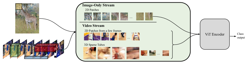
Figure 1: TubeViT: With Sparse Video Tubes, Vision Transformers (ViTs) use both image and video inputs, providing an efficient video backbone and more accurate performance.

To address these limitations, we propose a simple but effective model, named TubeViT, to utilize a standard ViT model seamlessly for both image and videos. We introduce Sparse Video Tubes, a lightweight approach for joint image and video learning. Our method works by sparsely sampling various sized 3D space-time tubes from the video to generate learnable tokens, which are used by the vision transformer (Figure 1). With sparse video tubes, the model is easily applicable to either input, and can better leverage either or both sources of data for training and fine-tuning. The sparse video tubes naturally handle raw video signals and image signals which is crucial to understanding actions and other spatio-temporal information in videos.

Video models are also expensive to train, and previous works have studied ways to leverage already trained models, such as using frozen ones [27] or adapting them to videos [31]. We expand on these ideas, and use the Sparse Video Tubes to adapt much larger ViT models to videos with lightweight training (Sec. 3.6). Thus we create powerful large video models with less resources.

We evaluate the approach across many standard video datasets: Kinetics-400, Kinetics-600, Kinetics-700, and SomethingSomething V2, outperforming the state-of-the-art (SOTA). Our methods are trained from scratch or on ImageNet-1k and Kinetics datasets and outperform even methods additionally pre-trained from very large datasets (e.g., JFT [46]). Our work also outperforms models targeting video pretraining, such as recent video Masked Auto-Encoder (MAE) works [47, 15].

Our key findings are that by using the sparse video tubes, we are able to better share the weights learned for both images and videos. This is in contrast to prior works that either inflate kernels or add new temporal-specific layers. Further, due to the sparse sampling, the number of tokens remains low, which we also find is important, both for reducing FLOPs and improving performance.

Our contribution is construction of sparse video tubes, obtained by sparsely sampling videos with various sized 3D space-time tubes. With that we accomplish the following: (1) a universal visual backbone which easily adapts a ViT architecture to videos; (2) joint image and video understanding which seamlessly uses either input; (3) an easy-to-scale approach for video understanding, which can also leverage already trained (large) ViT models.

2 Related work

Video understanding is an important topic in computer vision. Early works hand-designed trajectory features to understand motion and time [52]. With the success of neural networks, many different approaches have been developed, such as two-stream CNNs taking image frames plus optical flow for motion information as input [43], finding a clear benefit from adding the flow information. Works studying 3D CNNs found the learning of temporal kernels to be important [48, 8, 34, 50], but also required much more data in order to be effective [8]. Many of the existing video CNN approaches, have been specialized to handle videos, either with flow streams or 3D kernels and thus have not been applicable to images.

With the introduction of transformer models and self-attention [51], vision transformers have been very effective for image-based tasks. However, due to the quadratic cost of self-attention and the dense sampling, their use for videos has required different elements, such as space-time factorized attention [6, 3, 62]. However, these video transformers have not really been tested on longer videos and are mostly evaluated on short clips. The ability to handle larger number of input frames and understand long-term actions and their relationships is of key importance, but becomes computationally prohibitive with current models.

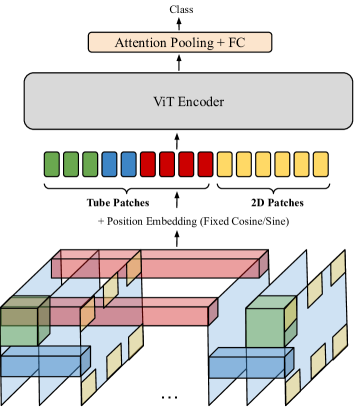
Figure 2: Illustration of the approach. We use tubes of different shapes to sparsely sample the video. These are concatenated together and used as input to a transformer model.

Previous works have found that transformers focus on only a few tokens [30, 37] and works have been designed to pool or reorganized tokens effectively [24, 38, 29]. Many video works have found that frames contain redundant information, and thus propose strategies to sample frames [17, 60]. Other works have studied ways to reduce the number of tokens in video transformer models [54, 32, 38]. However, all these works still use an initial dense sampling of the video, then some heuristics to reduce the number of inputs. In this work, we more sparsely sample the input initially, increasing efficiency.

Other recent works have studied video MAE tasks as pretraining [15, 47], they similarly treat videos as tubes, and study the sparseness in terms of the masking, having similar findings that sparseness is beneficial. However, they use a single tube shape and create non-overlapping patches and have not been studied when joint training with images.

This work is also related to approaches which use multiple views or streams from the input data, e.g., Multi-View Transformers [62], SlowFast Networks [16] and others [35, 43], all have found benefits from multiple input views or streams. MultiView Transformers [62], similarly to us, is using tubes of varying shapes. The key difference is the sparse sampling we use enables the use of a single ViT encoder model, rather than multiple smaller, per-view encoders. This further unifies the approach with images.

Another line of work in video understanding is leveraging image datasets during pre-training [12, 57]. This is valuable as image-only datasets are better annotated and provide richer semantic information. One approach is to bootstrap the video models from image-pretrained models, often by inflating kernels. The model is first pre-trained on image data, and then only trained on video. Other works proposed to co-train image and video jointly [57, 68, 25, 4, 53, 19]. These approaches adapt the architectures to handle both inputs which might be inefficient, e.g., treating an image input as a video of 1 frames [68] or using separate networks to first encode the inputs[19, 2].

In contrast to all the previous works, our method is simple and straightforward. One crucial set of differences is that the tubes are sparsely applied to the raw input, consists of different shaped, possibly overlapping tubes, and uses a single, shared backbone network, different from all previous approaches ([16, 62, 32, 38, 3, 15, 47]). This leads to both more efficient and accurate models. Secondly, and more importantly, the model is entirely shared between the image and video modalities. This is an important distinction as it not only improves performance for both tasks, but is also more generally applicable to vision tasks.

3 Method

3.1 Preliminaries

The standard ViT architecture [10] takes an image and converts it into patch embedding, for example, by using a $16\times 16$ 2D convolutional kernel, with a $16\times 16$ stride. This results in a sequence of patches as the image representation, e.g., 196 for a $224\times 224$ input image. Given a video $V\in\mathcal{R}^{T\times H\times W\times C}$, prior approaches either used the same, dense 2D patches (e.g., TimeSFormer [6]) or used dense 3D kernels, e.g., 2 or $4\times 16\times 16$ as in ViViT [3]. In both cases, this results in significantly more tokens, e.g., $T*196$, where $T$ is the number of frames. These tubes or patches are then linearly projected into an embedding space, $z_{i}\in\mathcal{R}^{d}$. This sequence of tokens is then processed by a transformer encoder, using standard components, MSA - the multi-head self attention and MLP - the standard transformer projection layer (LN denotes Layer Norm). For a sequence of layers $l\in[0,1,\ldots L]$, we compute the representation $y_{i}^{l}$ and next token features $z_{i}^{l}$ for all the $z_{i}$ tokens:

$$y_{i}^{l}=\text{MSA}(\text{LN}(z_{i}^{l-1}))+z_{i}^{l-1}$$ (1)

$$z_{i}^{l}=\text{MLP}(\text{LN}(y_{i}^{l}))+y_{i}^{l}$$ (2)

To reduce the computational cost, prior approaches factorize the attention mechanism, to have a spatial and temporal attention [3] or use multiple views with smaller, view level transformers [62].

3.2 Sparse Video Tubes

We propose a simple and straightforward method which is seamlessly applicable to both images and videos. Our approach follows the standard ViT tokenization approach for images: a 2D convolution with a $16\times 16$ kernel. We build on the observation that sparseness is effective for videos. Rather than following the prior works that densely tokenize the video, we instead use the same 2D kernel, but with a large temporal stride, for example, applied to every 16th frame. Thus for an input video clip of $32\times 224\times 224$, this results in only 392 tokens, rather than the  6k in TimeSFormer or 1-2k in ViViT.

However, this sparse spatial sampling might lose information, especially for quick or short actions. Thus, we create sparse tubes of different shapes, for example, a $16\times 4\times 4$ tube to obtain information from many frames at low spatial resolution. These tubes can have any shape, and we experimentally explore the effect of these. Importantly, these tubes also have large strides, sparsely sampling the video in different views. We also optionally add an offset to the start location, so that the patches do not always start at $(0,0,0)$ and this allows a reduction in the overlap between the tubes. This is illustrated in Figure 2. Tubes of various sizes are also used in the MultiView approach for video classification  [62], however there they are densely sampled and processed by multiple transformers, resulting in a more computationally intensive approach.

Furthermore, in contrast to prior works, we also allow for overlap between the tubes. Specifically, we can represent a tube as $(T\times H\times W)$ for the kernel shape, $(T_{s},H_{s},W_{s})$ for the spatio-temporal stride applied to the kernel, and $(x,y,z)$ as the offset of the starting point of the convolution.

With the proposed design, our approach enables seamless fusion of the image- and video- visual information. The sparse spatial sampling allows sharing the image and frame tokens and the sparse video tubes create a low number of video-specific tokens. This enables better sharing of the ViT model between images and videos.

3.3 Positional embedding for sparse video tubes

A key aspect of our approach is the implementation of the positional embedding. In language models, relative positional embeddings are a common and effective approach [51, 58]. However, here, the relative position between two tokens has minimal meaning, and no real reference to where the patch/tube came from in the original video or image. The ViT model [10] and similarly TimeSFormer [6] and ViViT [3] used learnable positional embeddings for the patches. Here, such an approach can be hard for the model, as these learned embeddings do not necessarily reflect where the patches came from in the original video, especially in the case where patches overlap.

Instead, we use a fixed sine/cosine embedding. Importantly, we take into account the stride, kernel shape and offsets of each tube when applying the positional embeddings. This ensures that the positional embedding of each patch and tube has the global spatio-temporal location of that tube.

Specifically, we compute the embeddings as follows. Here $\tau$ is a constant hyperparameter (we used 10,000). For $j$ from 0 to $d//6$ ($d$ is the number of features), and for $t,x,y$ from 0 to $T,H,W$, $z_{i}\in\mathcal{R}^{T\times H\times W\times D}$:

$$\omega_{j} =1/(\tau^{j})$$ (3)

$$p_{j,t} =\sin(t*\omega_{j}),\cos(t*\omega_{j})$$ (4)

$$p_{j,x} =\sin(x*\omega_{j}),\cos(x*\omega_{j})$$ (5)

$$p_{j,y} =\sin(y*\omega_{j}),\cos(y*\omega_{j})$$ (6)

$$z_{i}[t,x,y ,6j:6(j+1)]\mathrel{{+}{=}}[p_{j,t},p_{j,x},p_{j,y}]$$ (7)

This adds each spatio-temporal position embedding to the feature dimension of the token $z_{i}$. Following previous work [51], this is done for different wavelengths for each channel. $d//6$ is used since we have 6 elements (a sine and cosine value for each $x,y,t$), this creates a position value for each channel of the representation.

Importantly, here $z_{i}[t,x,y]$ represents the center of the tube, taking into account any strides and offsets used in the tube construction (the channel dimension is not shown here).

After the tokenization step, we concatenate all the tokens together and apply a standard transformer model. This simple structure lets the model share the majority of the weights between all inputs, which we find to be quite beneficial.

3.4 Sparse Tube Construction

We explore several methods to create the visual tubes. Our core approach consist of 2 tubes: the $1\times 16\times 16\times d$ tube used to tokenize the image and a $8\times 8\times 8\times d$ tube additionally used for the video. Both have strides of $16\times 16\times 16$. This base tokenizer provides strong performance, but we explore several variations on it.

Multi-Tube. We add multiple tubes to the core approach of various sizes. For example, we can add temporally long and spatially small tubes, such as $16\times 4\times 4$ to learn long actions, or more spatially focused tubes such as a $2\times 16\times 16$ tube. There are many variations of tube shape and stride, which we experimentally explore.

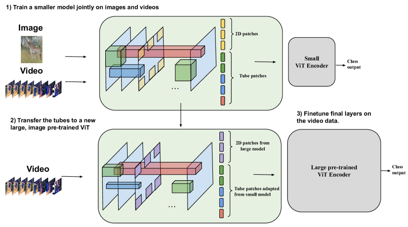
Figure 3: Scaling of TubeViT models: building large scale video models is expensive. We propose to expand model capacity for video models leveraging large pre-trained ViTs. With TubeViT we can easily train on both image and video data a small-scale model. Then we can adapt the sparse video tubes to a much larger image-only trained ViT, which can be mostly frozen.

Space-to-Depth Another way to extend the core approach is a method inspired by depth-to-space [41]. Here, we reduce the number of channels in a tube, e.g., by a factor of 2. Thus the tube shape becomes $T\times H\times W\times d/2$. Next, we concatenate 2 tokens along the channel axis. We can then also reduce the stride of the tube. This results in the same number of tokens and dimensions as the original, but effectively increases the kernel size without changing the number of parameters. I.e., when the stride is reduced on the time axis, the token now represents $T*2\times H\times W$ locations, but only uses $T*H*W$ parameters. In the experiments, we explore different settings: e.g., more temporal dense vs more spatially dense and the depth to space factor (2, 4, 8, etc.).

Interpolated Kernels. For this setting, rather than having a unique kernel for each tube, we learn 1 3D kernel of shape $8\times 8\times 8$. We then use tri-linear interpolation to reshape the kernel to various sizes, e.g., 4x16x16 or 32x4x4, etc. depending on the tube configuration. Any sized kernel can be created from this single kernel. This method has several advantages. (1) It reduces the number of learned parameters that are only used on the video stream. (2) It enables more flexible usage of the kernels, e.g., it can be made longer to handle longer videos, or spatially larger to find small objects.

The TubeViT approach consists of the union of the above-mentioned Multi-Tube and Space-to-Depth, the exact settings are provided in the supplemental materials. We experiment with Interpolated Kernels in ablations.

3.5 Image and Video Joint Training

As described above, our approach seamlessly adapts to either image, video or both inputs. While image+video joint inputs are rare, the ability to use them together while training is very important as many datasets with valuable annotations (e.g., ImageNet, Kinetics) come from either image sources or video sources but not both. Jointly training with our approach is easy – the image is tokenized by the 2D kernel and the video is tokenized by both the 2D patches (with large temporal stride) and Sparse Tubes. Both are then passed into a standard ViT; the position embedding will be supplied in either case. The position embedding approach is also needed for the joint training to be effective. We demonstrate the benefits of our approach for joint training in the experiments, Section 4.

3.6 Image-To-Video Scaling Up of Models

We also propose a method for a more efficient way of scaling up the models (Figure 3). Training large ViT models is computationally expensive, especially for videos. Since nearly all the components of our model are shared between the both images and videos, we explore a method to utilize large models without having heavy fine-tuning.

First, we train a smaller model jointly on images and videos. This gives us a set of weights for the tubes. Then we take a large pre-trained image ViT, but further add the tubes. These tubes use the same kernel weights as the smaller model, and so we can avoid further training them. Since larger ViTs generally use more channel dimensions than smaller ones, we use the space-to-depth transform again here to create tokens with the proper channel dimensions without needing new weights.

Next, we pick a point in the network and freeze all the layers before it, for example, the 26th of 32 layers in ViT-H. At this point, we add a gated connection to the network:

$$z^{s}=\text{MLP}(\text{LN}(y^{s}))+y^{s}+\tanh(\alpha)z^{0}$$ (8)

where $s$ is the layer the network is frozen at (e.g., 26) of the ViT model and $z^{0}$ is the raw input tokens from the tubes. $\alpha$ is the learned gating parameter, initialized at 0. In the first steps of training, this gate has no effect on the representation, and thus the ViT is unchanged. However, it can learn to incorporate the raw tubes at this point and further refine the later weights.

Method	PT Data	Top 1	Top 5	Crops	TFLOPs
TSM-ResNeXt-101 [26]	ImageNet-1k	76.3	–	–	–
I3D NL [56]	ImageNet-1k	77.7	93.3	$10\times 3$	10.77
VidTR-L [70]	ImageNet-1k	79.1	93.9	$10\times 3$	10.53
LGD-3D R101 [36]	ImageNet-lk	79.4	94.4	–	–
SlowFast R101-NL [16]	-	79.8	93.9	$10\times 3$	7.02
X3D-XXL [14]	-	80.4	94.6	$10\times 3$	5.82
OmniSource [12]	ImageNet-1k	80.5	94.4	–	–
TimeSformer-L [6]	ImageNet-21k	80.7	94.7	$1\times 3$	7.14
MFormer-HR [33]	ImageNet-21k	81.1	95.2	$10\times 3$	28.76
MViT-B [13]	-	81.2	95.1	$3\times 3$	4.10
MoViNet-A6 [21]	-	81.5	95.3	$1\times 1$	0.39
ViViT-L FE [3]	ImageNet-1k	81.7	93.8	$1\times 3$	11.94
MTV-B [62]	ImageNet-21K	82.4	95.2	$4\times 3$	11.16
VideoMAE [47]	-	87.4	97.6	-	-
Large Scale Pretraining Data
VATT-L [1]	HowTo100M	82.1	95.5	$4\times 3$	29.80
ip-CSN-152 [49]	IG-65M	82.5	95.3	$10\times 3$	3.27
R3D-RS [11]	WTS	83.5	–	$10\times 3$	9.21
OmniSource [12]	IG-65M	83.6	96.0	–	–
MAE-ST [15]	IG-1M	84.4	-	-	-
ViViT-H [3]	JFT	84.9	95.8	$4\times 3$	47.77
TokenLearner-L/10 [38]	JFT	85.4	96.3	$4\times 3$	48.91
Florence [65]	FLD-900M	86.5	97.3	$4\times 3$	–
CoVeR  [68]	JFT-3B	87.2	–	$1\times 3$	–
CoCa [64]	ALIGN (1.8B)	88.9	-	-	-
MTV-H [62]	WTS 280p	89.9	98.3	$4\times 3$	73.57
TubeVit-B	ImageNet-1k	88.6	97.6	$4\times 3$	0.87
TubeVit-L	ImageNet-1k	90.2	98.6	$4\times 3$	9.53
TubeViT-H (created)	ImageNet-1k	90.9	98.9	$4\times 3$	17.64

Table 1: Performance on Kinetics 400. TubeViT performs best. We report the crops and total TFLOPs used for inference. The crops, $t\times x$ denotes $t$ temporal and $x$ spatial crops.

Method	Top 1	Top 5
SlowFast R101-NL [16]	81.8	95.1
X3D-XL [14]	81.9	95.5
TimeSformer-L [6]	82.2	95.6
MFormer-HR [33]	82.7	96.1
ViViT-L FE [3]	82.9	94.6
MViT-B [13]	83.8	96.3
MoViNet-A6 [21]	84.8	96.5
R3D-RS [11] (WTS)	84.3	–
ViViT-H [3] (JFT)	85.8	96.5
TokenLearner-L/10 [38] (JFT)	86.3	97.0
Florence [65] (FLD-900M)	87.8	97.8
CoVeR [68] (JFT-3B)	87.9	–
MTV-H [62] (WTS 280p)	90.3	98.5
CoCa [64] (ALIGN 1.8B)	89.4	-
Merlot-Reserve-L [66] (YT-1B)	91.1	97.1
TubeVit-B (ImageNet-1k)	90.9	97.3
TubeVit-L (ImageNet-1k)	91.5	98.7
‘ TubeVit-H (created)	91.8	98.9

Table 2: Performance on Kinetics 600. Similarly, to Table 1 our model uses the ImageNet-1k dataset. Most models use significantly larger pre-training datasets (bottom half). Tube-ViT outperforms prior work.

	Top 1	Top 5
VidTR-L [70]	70.2	–
SlowFast R101 [16]	71.0	89.6
MoViNet-A6 [21]	72.3	–
CoVeR (JFT-3B) [68]	79.8	–
CoCa (Align 1.8B) [64]	82.7	-
MTV-H (WTS 280p) [62]	83.4	96.2
TubeViT-L	83.8	96.6

Table 3: Performance compared to SOTA on Kinetics 700.

	Top 1	Top 5
SlowFast R50 [16]	61.7	–
TimeSformer-L [6]	62.5
VidTR-L [70]	63.0	–
CoVeR [68]	64.7	–
MoViNet-A3 [21]	64.1	88.8
ViViT-L FE [3]	65.9	89.9
VoV3D-L [22]	67.3	90.5
MFormer-L [33]	68.1	91.2
MTV-B (320p) [62]	68.5	90.4
MViT-B [13]	68.7	91.5
MViT [23]	73.3	94.1
MaskFeat [59]	75.0	95.0
VideoMAE [47]	75.4	95.2
TubeViT-L	76.1	95.2

Table 4: Performance on Something-SomethingV2 dataset.

4 Experiments

We evaluate the approach on several popular datasets: Kinetics 400, Kinetics 600, Kinetics 700 [20, 7], and SomethingSomething V2 [18]. These datasets cover a wide variety of video understanding challenges and are well established in the literature. The main results are trained jointly on ImageNet-1k (of 1.2M images) and the video data, please see the supplemental materials for full details. We use standard Top 1 and Top 5 evaluation metrics and report FLOPs of ours and previous works, when available. Our model sizes are 90M Base (B), 311M Large (L). A 635M Huge (H) is ‘created’ with Image-to-Video scaling.

4.1 Main results

For the main results, we use 4 tubes with the following configuration (order of $t,h,w$): (1) $8\times 8\times 8$ with a stride of $(16,32,32)$; (2) $16\times 4\times 4$ with a stride of $6\times 32\times 32$ and an offset of $(4,8,8)$; (3) $4\times 12\times 12$ with a stride of $(16,32,32)$ and an offset of $(0,16,16)$; and (4) $1\times 16\times 16$ with a stride of $(32,16,16)$. For an input of $32\times 224\times 224$, this results in only 559 tokens, significantly less than other approaches. In the supplemental material, we have detailed experiments over many tube configurations, as well as the space-to-depth settings used.

We would like to note that with data augmentation such as random spatial and temporal cropping, over multiple training epochs the model will see different parts of the video, even with sparse sampling.

Comparison to SOTA. First, we compare our final approach to previous state-of-the-art (SOTA) methods. Tables 1, 2 and 3 shows the performance of our model compared to the state-of-the-art on the Kinetics-400 Kinetics-600 and Kinetics-700 datasets. Table 1 shows additional information (e.g. views, pre-training datasets) which applies to the other tables as well. These results show our approach outperforms SOTA, both in terms of accuracy and efficiency. We also outperform methods on co-training of images and videos, and methods with strong video pre-training.

We note that all the sizes of our model perform well, despite the fact that others are much larger or use significantly larger pre-training data (e.g., CoCa with 1B params and 1.8B examples, MerlotReserve has 644M params and uses YT-1B dataset). Table 4 shows our results on the Something-Something dataset (SSv2). This dataset is often used to evaluate more dynamic activities. Our approach outperforms SOTA on it as well.

Joint image+video training. We further explore the effects of co-training on image+video datasets, finding this to be highly effective as also shown above. Table 5 evaluates this in a side-by-side experiment of using Kinetics (video) only vs Kinetics and ImageNet datasets for pre-training. We see that there is a large gain from the co-training of our approach. We see that two-stage training, i.e., first training on one dataset and then training on a second one, is also weaker than the joint training, as the two datasets cannot interact during training. We also compare to prior methods such as TimeSFormer [6] only using dense 2D patches, or using inflated 3D kernels (e.g., ViViT [3]). In both cases, we see a clear benefit from the proposed approach. We also note that these prior approaches have significantly more FLOPs, due to the large number of tokens from the dense sampling. Our observations that image and video co-training is beneficial are consistent with prior works [68, 25]; here the difference is that we have a single compact model to do that.

As a sanity check, we also compare our performance on ImageNet-1k, without any hyperparameter tuning or additions: our ViT-B model only trained on ImageNet has 78.1 accuracy, similar to the ViT-B in [44]. When joint training with Kinetics-600, the model gets 81.4, a gain of 3.4%, showing the benefits of joint training for image-only tasks too. While other works achieve higher performance on ImageNet, they often use specialized data augmentation, learning schedules, and other tricks which we are not using. Instead, we are purely studying the benefit from using both videos and images.

	Kinetics 600
TubeViT-L Kinetics-only	85.6
TubeViT-L ImageNet then Kinetics	90.4
TubeViT-L ImageNet+Kinetics Jointly	91.5
2D Patches only ImageNet+Kinetics	87.6
Inflated 3D Patches ImageNet then Kinetics	88.4

Table 5: Combining datasets, which TubeViT seamlessly allows, is highly effective, as seen here in these side-by-side results for the Kinetics-600 dataset. The results are based on the ViT-L model.

Scaling video training with sparse video tubes. In Table 6 we demonstrate how a small TubeViT model can be adapted leveraging a large and (often independently) pre-trained model on images only. We start by leveraging a large, image-pretrained ViT, here ViT-H. We then take the learned tubes from TubeViT-B and use them along with the ViT-H image tokenizer to generate a set of tokens from a video, same as before. Then these are used as input to ViT-H, and we finetune only the latter parts of the model on the video data. These results suggests that this is an effective way to scale and utilize giant ViT models without needing the high compute cost to fully finetune the model. We also see that the gating in Eq. 8 is effective. We also found that in this setting, training time was reduced by 43%, as it has fewer weights to update.

Models	K600, Accuracy (%)
TubeViT-H Full Finetune	91.8
Scaling method with different portions trained
Last FC Layer	85.6
+ Last 4 Layers	86.3
+ Last 8 Layers	86.8
+ Last 8 + Gated (Eq. 8)	89.7

Table 6: Image-to-Video Scaling. We take a ImageNet pre-trained ViT-H and use a set of Tubes from TubeViT-B to create the tokens. We then fine-tune different portions of the model to see how we can best take advantage of existing, large pretrained ViT models. Even pretraining of handful of layers can achieve performance approaching the full model training.

Detrimental Effects of Too Many Tokens. Next we study the effect of number of tokens used in the model, shown in Figure 4. This result is another key insight as to why our approach works so well: with too many tokens, the performance drops, especially when only using Kinetics data. There are a number of possible reasons for why this occurs, for example, the self-attention mechanism could be struggling to learn for longer sequences, or there may not be sufficient data to learn the longer sequences, or perhaps the model is overfitting with longer sequences. This result indicates that for current datasets, the sparse sampling is an effective and efficient way to process videos. Further, it is possible that existing using long, densely sampled sequences are effected by this, and perhaps another reason the factorized attention modules are needed.

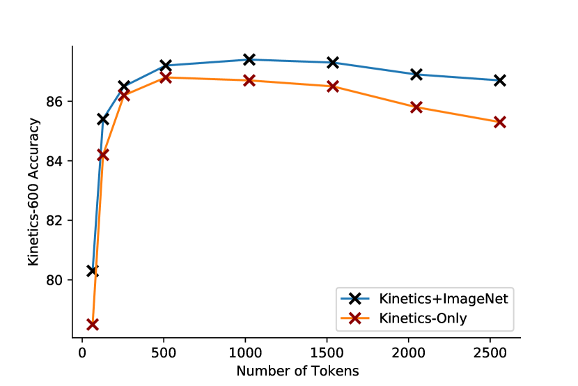
Figure 4: Accuracy vs. Number of tokens used in our model. We find that when increasing the tokens above 1500, there is a noticeable drop in performance, especially when only training on Kinetics-600 data. Joint training is more robust.

4.2 Ablations

In this section, we present a number of ablation studies to determine why this method is effective. For these experiments we use Kinetics 600.

Main ablations. First, we study the effect of the choice of position biases (Table 7a). We find that adding fixed cosine position embedding performs best and much better than other embeddings. Intuitively, this makes sense, since we are sparsely sampling potentially overlapping tokens, this method is able to best capture the token location.

Next in Table 7b, we study the number of tubes used. This finding, which is consistent with previous multi-view observations [62], shows that having a variety of tubes is beneficial to video understanding.

Next, in Table 7c, we study the depth-to-space versions of the network. Here, we reduce the channels of the generated tokens from $D//S$, e.g., by a factor of 2 or 4. Then after generating the tokens, we concatenate them along the channel axis. We study both increasing the number of tokens along the spatial and temporal dimensions. We find this to be an effective method, as it enables more dense samples without increasing the number of parameters or tokens.

Table 7d compares evaluating with more patches than the model was trained with. To do this we reduce the strides of the kernel. Initially this improves results, but after increasing 2x, the performance begins to drop, likely because the evaluation data is too different from the training one.

In Table 7e, we study the ability of the interpolated single kernel. I.e., rather than having $N$ 3D convolutional kernels, one for each tube, we build 1 $8\times 8\times 8$ 3D kernel and use interpolation to generate the different tube shapes. Somewhat surprisingly, we find this works fairly well, while also reducing the number of learnable parameters in the network.

In Table 7f, we compare the approach with different number of temporal and spatial crops. We find that even a single crop gives strong performance, and the standard $4\times 3$ performs nearly the same as the $10\times 10$ setting, suggesting that the sparse samples are quite suitable and further information is not as beneficial.

	K600
None	78.6
Learned	79.2
Relative	77.5
Fixed Cosine (no stride)	77.7
Fixed Cosine (Ours)	84.5

(a) Position Embeddings. Fixed, cosine embeddings with strides is best.

	GF	K600
1	70	78.4
2	71	81.5
4	72	83.4
8	74	85.4

(b) Number of Tubes.

	GF	K600
Baseline	72	83.4
With D2S x2 T	72	84.7
With D2S x2 S	72	84.5
With D2S x4 T	72	85.1
With D2S x4 S	72	85.4
With D2S x4 ST	72	85.3

(c) Space To Depth. Applying space-to-depth temporally (T), spatially (S), and spatio-temporally (ST).

	K600
Base (559)	84.5
768	84.9
1024	84.6
1536	83.5

(d) Eval Tokens. Generating larger number of tokens at eval time than in training, where 559 are used.

	K600
Interpolated	83.8
TubeViT	84.5

(e) Interpolated Kernel. Using a single 3D kernel interpolated to different sizes.

	K600
$1\times 1$	82.8
$4\times 1$	83.3
$1\times 3$	83.6
$4\times 3$	84.5
$10\times 10$	84.7

(f) Multi-Crop Evaluation. $4\times 3$ is used in the paper.

Table 7: Ablation studies on various components of our approach on Kinetics-600, using TubeViT-B.

Factorized attention ablations. In Table 8, we further study the effect of adding a new attention layer to an ImageNet pre-trained ViT model. Here, we are using the tube method to tokenize the inputs, but instead of using a factorized attention module, we simply add an additional self-attention layer. This has a similar effect of the factorized attention approaches that add new, uninitialized $K,Q,V$ projections to a pre-trained ViT (e.g., TimeSFormer and ViViT). These results indicate that such methods are not able to best utilize the image pre-trained weights of the network due to these new layers. Since the sparse tubes yield few additional tokens, they can directly use the same ViT model without factorized attention and are thus able to better utilize the image trained weights. Note that there are still differences between the works, e.g., the reduced number of tokens, etc. However, we believe this observation holds, and is a possible explanation for why the spatio-temporal attention in ViVit performed better for some datasets.

Layers Added	K600
0	84.23
1	80.23
2	78.87
4	75.24
8	72.95

Table 8: We find that adding even a single layer to a pretrained image network degrades performance. This suggests that the factorized attention methods are sub-optimal since they cannot fully take advantage of the image-pre-trained networks. Trained for 70k steps.

Model scaling ablations. Table 9 provides ablations on scaling to create TubeViT Base from a Tiny one. Even just training the final few layers is effective (4 of 12), and can nearly match the performance of full finetuning. This is consistent with our observations in Table 6 for ViT-H.

Trained	K600
Last FC Layer	79.6
+ 1 Layer	80.8
+ 4 Layers	81.1
Whole Model	81.4

Table 9: Image-to-Video scaling from Tiny to Base. We take a ImageNet pre-trained ViT-Base and the TubeViT corresponding to ViT-Tiny and ImageNet pre-trained ViT-Base to create a larger TubeViT. These models were trained for 50k steps.

Figure 5 visualizes the learned 2D patches and 3D tubes.

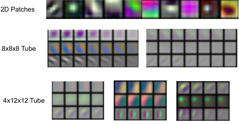
Figure 5: Visualization of a selected set of 2D patches and tubes.

5 Conclusion

We proposed sparse video tubes for video recognition. With sparse video tubes, a ViT encoder can be transformed into an efficient video model. The approach is simple, enables seamless joint training with images and videos and improves video recognition across multiple datasets. We also demonstrate an elegant scaling of video models with our proposed method. We conduct extensive ablation experiments to determine why the approach works, finding the a combination of the joint training, reduced tokens, and better utilization of shared image+video weights led to the improvements. We obtain SOTA or above performance.

Appendix A Implementation Details

Our hyperparameters are summarized in Table 10. For all datasets, we employ random spatial and temporal cropping. For most datasets, these settings were the same. For Charades, we decreased the batch size but used longer, 128 frame clips, as Charades videos are roughly 30 seconds long, compared to 10 seconds for Kinetics.

We also found some training instability when using larger ViT models. When using ViT-L or ViT-H models, we had to decrease the weight decay value as well as the learning rate, otherwise we found the training accuracy dropped to 0 and the loss stayed flat.

For smaller datasets, such as Charades and SSv2, we had to increase the data augmentation settings, as done in previous works, e.g., [62]. We added Mixup and label smoothing and dropout to them.

For all the datasets, we applied RandAugment [9], as we found this to be beneficial. We also kept the number of steps the same for all datasets.

	K400	K600	K700	Charades	SSv2
Optimization
Optimizer	Adam
Batch size	256	256	256	64	256
Learning rate schedule	cosine decay + linear warmup
Linear warmup steps	10,000
Base learning rate	5e-5 (L,H 1e-5)			1e-3	2e-5
Steps	300,000
Data augmentation
Rand augment number of layers [9]	2
Rand augment magnitude [9]	10
Weight Decay	0.001 (B) 1e-5 (L,H)
Mixup [69]	-	-	-	-	0.3
Dropout	-	-	-	0.2	0.3
Label Smoothing	-	-	-	0.1	0.3
Number of Frames	64	64	64	128	32
FPS	15	15	15	6	24

Table 10: Training hyperparamters for our experiments. We note when different settings were used for the base (B), large (L) and huge (H) models.

Joint ImageNet and Kinetics Training. When jointly training on the two (or more) datasets, we use a separate fully connected layer to output the class predictions. E.g., for ImageNet and Kinetics-600, we use an FC layer with 1,000 and 600 outputs. We then compute the loss for the relevant head and backpropagate it. During the joint training, we use the same settings as listed in Table 10. We use the joint training for Kinetics 400, 600 and 700. For Charades and SSv2, we use the Kinetics-600+ImageNet pretrained model and finetune it on the dataset.

Full Model Settings. Our model is based on the standard ViT models, thus the core of the approach is the same as previous ViTs [10]. We summarize those settings in Table 11.

Model	Layers	Hidden size $d$	MLP size	Num Heads	Params
ViT-Base	12	768	3072	12	86M
ViT-Large	24	1024	4096	16	307M
ViT-Huge	32	1280	5120	16	632M

Table 11: Parameter count for the vit encoder backbones.

In Table 12, we detail the settings for each tube.

Kernel	Stride	Offset	S2D	params
$8\times 8\times 8$	$(16,32,32)$	(0, 0, 0)	2x temporal	$512d$
$16\times 4\times 4$	$(6,32,32)$	(4, 8, 8)	4x spatial	$256d$
$4\times 12\times 12$	$(16,32,32)$	(0, 16, 16)	-	$576d$
$1\times 16\times 16$	$(32,16,16)$	(0, 0, 0)	-	$256d$

Table 12: Configuration for the tubes using the in main Tube-ViT. We also report the number of params used by each tube, which depends on $d$, the hidden size of the ViT model used. The tubes add an additional 1-3M params, depending on the model, a small fraction of the total model size.

Appendix B Additional Experiments on Charades

We include results on Charades [42] to show the effectiveness of this approach on longer videos, since Charades videos are on average 30 seconds long. However, Charades is also a multi-label dataset, and we found it required different settings to effectively train, so we include all those details here.

First, we found that the core multi-tube approach were not performing as well as some prior work (e.g., AssembleNet [39]). Since Charades has a lot of object-related actions and contains longer videos with more temporal information, we modified the core model to make it more suitable for this data. First, we used the interpolation method to increase the tube shapes to:

• $1\times 16\times 16$

• $16\times 16\times 16$

• $32\times 8\times 8$

• $4\times 32\times 32$

We note two important factors. First, since we use interpolation to create the larger kernels, the number of learned parameters is the same, and initialized from the same kernels for the other datasets. Second, since the number of strides is unchanged, this results is the same number of tokens. Critically, this change has very little effect on the network and its parameters, but enables the model to better capture the information for Charades.

In Table 13, we report the results. The core MultiTube approach performs quite well, but with the interpolated kernels, is able to perform on par with TokenLearner [38], the state-of-the-art, while still sparsely sampling the video. We also perform similarly using significantly less data, e.g., JFT-300M was used to pre-trained TokenLearner, we accomplish the same performance without such large scale data.

	mAP
SlowFast [16]	45.2
AssembleNet-101 [40]	58.6
AssembleNet++-50 [39]	59.8
MoViNet-A6 [21]	63.2
TokenLearner [38]	66.3
MultiTube Tube-ViT-L	61.8
Interpolated TubeViT-L	66.2

Table 13: Charades classification.

Appendix C Ablations on Tube Shapes.

In Table 14, we provide a detailed study on Kinetics-600 of various tube configurations. We observe that the model isn’t overly sensitive to tube shapes, at least on Kinetics-600, but having multiple, different tubes, as well as variation in their shapes is generally beneficial. We use the following tubes in these experiments:

1. $1\times 16\times 16$

2. $4\times 32\times 32$

3. $4\times 4\times 4$

4. $4\times 12\times 12$

5. $8\times 8\times 8$

6. $16\times 4\times 4$

7. $16\times 16\times 16$

8. $32\times 8\times 8$

and the following strides:

1. (4, 16, 16)

2. (8, 8, 8)

3. (8, 32, 32)

4. (16, 16, 16)

5. (32, 32, 32)

Tube Config	K600
(a+iv) + (b+v) + (f+iv)	87.9
(c+iv) + (e+v) + (g+iv)	87.5
(a+iv) + (e+v) + (g+iv)	87.8
(b+iv) + (e+v) + (g+iv)	87.7
(a+iv) + (d+v) + (e+iv) + (h+v)	88.6
(a+iv) + (b+v) + (c+iv) + (h+v)	87.9
(a+iv) + (d+v) + (e+iv) + (f+v)	88.9

Table 14: Ablation on different tube shapes, trained for 50k steps.

References

- [1] Hassan Akbari, Linagzhe Yuan, Rui Qian, Wei-Hong Chuang, Shih-Fu Chang, Yin Cui, and Boqing Gong. Vatt: Transformers for multimodal self-supervised learning from raw video, audio and text. In NeurIPS, 2021.
- [2] Jean-Baptiste Alayrac, Jeff Donahue, Pauline Luc, Antoine Miech, Iain Barr, Yana Hasson, Karel Lenc, Arthur Mensch, Katie Millican, Malcolm Reynolds, Roman Ring, Eliza Rutherford, Serkan Cabi, Tengda Han, Zhitao Gong, Sina Samangooei, Marianne Monteiro, Jacob Menick, Sebastian Borgeaud, Andrew Brock, Aida Nematzadeh, Sahand Sharifzadeh, Mikolaj Binkowski, Ricardo Barreira, Oriol Vinyals, Andrew Zisserman, and Karen Simonyan. Flamingo: a visual language model for few-shot learning, 2022.
- [3] Anurag Arnab, Mostafa Dehghani, Georg Heigold, Chen Sun, Mario Lučić, and Cordelia Schmid. Vivit: A video vision transformer. In ICCV, 2021.
- [4] Max Bain, Arsha Nagrani, Gül Varol, and Andrew Zisserman. Frozen in time: A joint video and image encoder for end-to-end retrieval. In ICCV, 2021.
- [5] Hangbo Bao, Li Dong, Songhao Piao, and Furu Wei. Beit: Bert pre-training of image transformers. In arXiv:https://arxiv.org/abs/2106.08254, 2021.
- [6] Gedas Bertasius, Heng Wang, and Lorenzo Torresani. Is space-time attention all you need for video understanding? In ICML, 2021.
- [7] Joao Carreira, Eric Noland, Chloe Hillier, and Andrew Zisserman. A short note on the kinetics-700 human action dataset. In arXiv preprint arXiv:1907.06987, 2019.
- [8] Joao Carreira and Andrew Zisserman. Quo vadis, action recognition? a new model and the kinetics dataset. In CVPR, 2017.
- [9] Ekin D. Cubuk, Barret Zoph, Jonathon Shlens, and Quoc V. Le. Randaugment: Practical automated data augmentation with a reduced search space. In NeurIPS, 2020.
- [10] Alexey Dosovitskiy, Lucas Beyer, Alexander Kolesnikov, Dirk Weissenborn, Xiaohua Zhai, Thomas Unterthiner, Mostafa Dehghani, Matthias Minderer, Georg Heigold, Sylvain Gelly, Jakob Uszkoreit, and Neil Houlsby. An image is worth 16x16 words: Transformers for image recognition at scale. In ICLR, 2021.
- [11] Xianzhi Du, Yeqing Li, Yin Cui, Rui Qian, Jing Li, and Irwan Bello. Revisiting 3d resnets for video recognition. In arXiv preprint arXiv:2109.01696, 2021.
- [12] Haodong Duan, Yue Zhao, Yuanjun Xiong, Wentao Liu, and Dahua Lin. Omni-sourced webly-supervised learning for video recognition. In ECCV, 2020.
- [13] Haoqi Fan, Bo Xiong, Karttikeya Mangalam, Yanghao Li, Zhicheng Yan, Jitendra Malik, and Christoph Feichtenhofer. Multiscale vision transformers. In ICCV, 2021.
- [14] Christoph Feichtenhofer. X3d: Expanding architectures for efficient video recognition. In CVPR, 2020.
- [15] Christoph Feichtenhofer, Haoqi Fan, Yanghao Li, and Kaiming He. Masked autoencoders as spatiotemporal learners. arXiv preprint arXiv:2205.09113, 2022.
- [16] Christoph Feichtenhofer, Haoqi Fan, Jitendra Malik, and Kaiming He. Slowfast networks for video recognition. In ICCV, 2019.
- [17] Shreyank N Gowda, Marcus Rohrbach, and Laura Sevilla-Lara. Smart frame selection for action recognition. In Proceedings of the AAAI Conference on Artificial Intelligence, volume 35, pages 1451–1459, 2021.
- [18] Raghav Goyal, Samira Ebrahimi Kahou, Vincent Michalski, Joanna Materzynska, Susanne Westphal, Heuna Kim, Valentin Haenel, Ingo Fruend, Peter Yianilos, Moritz Mueller-Freitag, et al. The” something something” video database for learning and evaluating visual common sense. In ICCV, 2017.
- [19] Andrew Jaegle, Sebastian Borgeaud, Jean-Baptiste Alayrac, Carl Doersch, Catalin Ionescu, David Ding, Skanda Koppula, Daniel Zoran, Andrew Brock, Evan Shelhamer, Olivier Hénaff, Matthew M. Botvinick, Andrew Zisserman, Oriol Vinyals, and João Carreira. Perceiver io: A general architecture for structured inputs & outputs. In arXiv preprint arXiv: 2107.14795, 2021.
- [20] Will Kay, Joao Carreira, Karen Simonyan, Brian Zhang, Chloe Hillier, Sudheendra Vijayanarasimhan, Fabio Viola, Tim Green, Trevor Back, Paul Natsev, et al. The kinetics human action video dataset. In arXiv preprint arXiv:1705.06950, 2017.
- [21] Dan Kondratyuk, Liangzhe Yuan, Yandong Li, Li Zhang, Mingxing Tan, Matthew Brown, and Boqing Gong. Movinets: Mobile video networks for efficient video recognition. In CVPR, 2021.
- [22] Youngwan Lee, Hyung-Il Kim, and Jinyoung Moon Kimin Yun. Diverse temporal aggregation and depthwise spatiotemporal factorization for efficient video classification. In arXiv preprint arXiv:2012.00317, 2020.
- [23] Yanghao Li, Chao-Yuan Wu, Haoqi Fan, Karttikeya Mangalam, Bo Xiong, Jitendra Malik, and Christoph Feichtenhofer. Mvitv2: Improved multiscale vision transformers for classification and detection. In Proceedings of the IEEE/CVF Conference on Computer Vision and Pattern Recognition, pages 4804–4814, 2022.
- [24] Youwei Liang, Chongjian Ge, Zhan Tong, Yibing Song, Jue Wang, and Pengtao Xie. Not all patches are what you need: Expediting vision transformers via token reorganizations. arXiv preprint arXiv:2202.07800, 2022.
- [25] Valerii Likhosherstov, Anurag Arnab, Krzysztof Choromanski, Mario Lucic, Yi Tay, Adrian Weller, and Mostafa Dehghani. Polyvit: Co-training vision transformers on images, videos and audio. arXiv preprint arXiv:2111.12993, 2021.
- [26] Ji Lin, Chuang Gan, and Song Han. Tsm: Temporal shift module for efficient video understanding. In ICCV, 2019.
- [27] Ziyi Lin, Shijie Geng, Renrui Zhang, Peng Gao, Gerard de Melo, Xiaogang Wang, Jifeng Dai, Yu Qiao, and Hongsheng Li. Frozen clip models are efficient video learners. In European Conference on Computer Vision, pages 388–404. Springer, 2022.
- [28] Ze Liu, Jia Ning, Yue Cao, Yixuan Wei, Zheng Zhang, Stephen Lin, and Han Hu. Video swin transformer. In arXiv preprint arXiv:2106.13230, 2021.
- [29] Dmitrii Marin, Jen-Hao Rick Chang, Anurag Ranjan, Anish Prabhu, Mohammad Rastegari, and Oncel Tuzel. Token pooling in vision transformers. arXiv preprint arXiv:2110.03860, 2021.
- [30] Muhammad Muzammal Naseer, Kanchana Ranasinghe, Salman H Khan, Munawar Hayat, Fahad Shahbaz Khan, and Ming-Hsuan Yang. Intriguing properties of vision transformers. Advances in Neural Information Processing Systems, 34:23296–23308, 2021.
- [31] Bolin Ni, Houwen Peng, Minghao Chen, Songyang Zhang, Gaofeng Meng, Jianlong Fu, Shiming Xiang, and Haibin Ling. Expanding language-image pretrained models for general video recognition. In ECCV, 2022.
- [32] Seong Hyeon Park, Jihoon Tack, Byeongho Heo, Jung-Woo Ha, and Jinwoo Shin. K-centered patch sampling for efficient video recognition. In European Conference on Computer Vision, pages 160–176. Springer, 2022.
- [33] Mandela Patrick, Dylan Campbell, Yuki M Asano, Ishan Misra Florian Metze, Christoph Feichtenhofer, Andrea Vedaldi, Jo Henriques, et al. Keeping your eye on the ball: Trajectory attention in video transformers. In NeurIPS, 2021.
- [34] AJ Piergiovanni, Anelia Angelova, Alexander Toshev, and Michael S Ryoo. Evolving space-time neural architectures for videos. In Proceedings of the IEEE/CVF International Conference on Computer Vision, pages 1793–1802, 2019.
- [35] AJ Piergiovanni, Kairo Morton, Weicheng Kuo, Michael Ryoo, and Anelia Angelova. Video question answering with iterative video-text co-tokenization. ECCV, 2022.
- [36] Zhaofan Qiu, Ting Yao, Chong-Wah Ngo, Xinmei Tian, and Tao Mei. Learning spatio-temporal representation with local and global diffusion. In CVPR, 2019.
- [37] Yongming Rao, Wenliang Zhao, Benlin Liu, Jiwen Lu, Jie Zhou, and Cho-Jui Hsieh. Dynamicvit: Efficient vision transformers with dynamic token sparsification. Advances in neural information processing systems, 34:13937–13949, 2021.
- [38] Michael S. Ryoo, AJ Piergiovanni, Anurag Arnab, Mostafa Dehghani, and Anelia Angelova. Tokenlearner: Adaptive space-time tokenization for videos. 2021.
- [39] Michael S Ryoo, AJ Piergiovanni, Juhana Kangaspunta, and Anelia Angelova. Assemblenet++: Assembling modality representations via attention connections. In European Conference on Computer Vision, pages 654–671. Springer, 2020.
- [40] Michael S Ryoo, AJ Piergiovanni, Mingxing Tan, and Anelia Angelova. Assemblenet: Searching for multi-stream neural connectivity in video architectures. In ICLR, 2019.
- [41] Wenzhe Shi, Jose Caballero, Ferenc Huszár, Johannes Totz, Andrew P Aitken, Rob Bishop, Daniel Rueckert, and Zehan Wang. Real-time single image and video super-resolution using an efficient sub-pixel convolutional neural network. In Proceedings of the IEEE conference on computer vision and pattern recognition, pages 1874–1883, 2016.
- [42] Gunnar A Sigurdsson, Gül Varol, Xiaolong Wang, Ali Farhadi, Ivan Laptev, and Abhinav Gupta. Hollywood in homes: Crowdsourcing data collection for activity understanding. In European Conference on Computer Vision, pages 510–526. Springer, 2016.
- [43] Karen Simonyan and Andrew Zisserman. Two-stream convolutional networks for action recognition in videos. In NeurIPS, 2014.
- [44] Andreas Steiner, Alexander Kolesnikov, , Xiaohua Zhai, Ross Wightman, Jakob Uszkoreit, and Lucas Beyer. How to train your vit? data, augmentation, and regularization in vision transformers. In arXiv preprint arXiv:2106.10270, 2021.
- [45] Robin Strudel, Ricardo Garcia, Ivan Laptev, and Cordelia Schmid. Segmenter: Transformer for semantic segmentation. In ICCV, 2021.
- [46] Chen Sun, Abhinav Shrivastava, Saurabh Singh, and Abhinav Gupta. Revisiting unreasonable effectiveness of data in deep learning era. In ICCV, 2017.
- [47] Zhan Tong, Yibing Song, Jue Wang, and Limin Wang. Videomae: Masked autoencoders are data-efficient learners for self-supervised video pre-training. arXiv preprint arXiv:2203.12602, 2022.
- [48] Du Tran, Lubomir Bourdev, Rob Fergus, Lorenzo Torresani, and Manohar Paluri. Learning spatiotemporal features with 3d convolutional networks. In ICCV, 2015.
- [49] Du Tran, Heng Wang, Lorenzo Torresani, and Matt Feiszli. Video classification with channel-separated convolutional networks. In ICCV, 2019.
- [50] Du Tran, Heng Wang, Lorenzo Torresani, Jamie Ray, Yann LeCun, and Manohar Paluri. A closer look at spatiotemporal convolutions for action recognition. In CVPR, 2018.
- [51] Ashish Vaswani, Noam Shazeer, Niki Parmar, Jakob Uszkoreit, Llion Jones, Aidan N Gomez, Łukasz Kaiser, and Illia Polosukhin. Attention is all you need. In NeurIPS, 2017.
- [52] Heng Wang and Cordelia Schmid. Action recognition with improved trajectories. In Proceedings of the IEEE international conference on computer vision, pages 3551–3558, 2013.
- [53] Junke Wang, Dongdong Chen, Zuxuan Wu, Chong Luo, Luowei Zhou, Yucheng Zhao, Yujia Xie, Ce Liu, Yu-Gang Jiang, and Lu Yuan. Omnivl: One foundation model for image-language and video-language tasks. 2022.
- [54] Junke Wang, Xitong Yang, Hengduo Li, Li Liu, Zuxuan Wu, and Yu-Gang Jiang. Efficient video transformers with spatial-temporal token selection. In European Conference on Computer Vision, pages 69–86. Springer, 2022.
- [55] Wenhai Wang, Enze Xie, Xiang Li, Kaitao Song Deng-Ping Fan, Ding Liang, Tong Lu, Ping Luo, and Ling Shao. Pyramid vision transformer: A versatile backbone for dense prediction without convolutions. In ICCV, 2021.
- [56] Xiaolong Wang, Ross Girshick, Abhinav Gupta, and Kaiming He. Non-local neural networks. In CVPR, 2018.
- [57] Yufei Wang, Du Tran, and Lorenzo Torresani. Unidual: A unified model for image and video understanding. In arXiv preprint arXiv:1906.03857, 2019.
- [58] Yu-An Wang and Yun-Nung Chen. What do position embeddings learn? an empirical study of pre-trained language model positional encoding. arXiv preprint arXiv:2010.04903, 2022.
- [59] Chen Wei, Haoqi Fan, Saining Xie, Chao-Yuan Wu, Alan Yuille, and Christoph Feichtenhofer. Masked feature prediction for self-supervised visual pre-training. In arXiv:https://arxiv.org/abs/2112.09133, 2021.
- [60] Zuxuan Wu, Caiming Xiong, Chih-Yao Ma, Richard Socher, and Larry S Davis. Adaframe: Adaptive frame selection for fast video recognition. In Proceedings of the IEEE/CVF Conference on Computer Vision and Pattern Recognition, pages 1278–1287, 2019.
- [61] Saining Xie, Chen Sun, Jonathan Huang, Zhuowen Tu, and Kevin Murphy. Rethinking spatiotemporal feature learning: Speed-accuracy trade-offs in video classification. In ECCV, 2018.
- [62] Shen Yan, Xuehan Xiong, Anurag Arnab, Zhichao Lu, Mi Zhang, Chen Sun, and Cordelia Schmid. Multiview transformers for video recognition. In CVPR, 2022.
- [63] Lewei Yao, Runhui Huang, Lu Hou, Guansong Lu, Minzhe Niu, Hang Xu, Xiaodan Liang, Zhenguo Li, Xin Jiang, and Chunjing Xu. Filip: Fine-grained interactive language-image pre-training. ICLR, 2022.
- [64] Jiahui Yu, Zirui Wang, Vijay Vasudevan, Legg Yeung, Mojtaba Seyedhosseini, and Yonghui Wu. Coca: Contrastive captioners are image-text foundation models, 2022.
- [65] Lu Yuan, Dongdong Chen, Yi-Ling Chen, Noel Codella, Xiyang Dai, Jianfeng Gao, Houdong Hu, Xuedong Huang, Boxin Li, Chunyuan Li, et al. Florence: A new foundation model for computer vision. In arXiv preprint arXiv:2111.11432, 2021.
- [66] Rowan Zellers, Jiasen Lu, Ximing Lu, Youngjae Yu, Yanpeng Zhao, Mohammadreza Salehi, Aditya Kusupati, Jack Hessel, Ali Farhadi, and Yejin Choi. Merlot reserve: Neural script knowledge through vision and language and sound. In Proceedings of the IEEE/CVF Conference on Computer Vision and Pattern Recognition, pages 16375–16387, 2022.
- [67] Xiaohua Zhai, Alexander Kolesnikov, and Lucas Beyer Neil Houlsby. Scaling vision transformers. In CVPR, 2022.
- [68] Bowen Zhang, Jiahui Yu, Christopher Fifty, Wei Han, Andrew M Dai, Ruoming Pang, and Fei Sha. Co-training transformer with videos and images improves action recognition. In arXiv preprint arXiv:2112.07175, 2021.
- [69] Hongyi Zhang, Moustapha Cisse, Yann N. Dauphin, and David Lopez-Paz. Mixup: Beyond empirical risk minimization. In ICLR, 2018.
- [70] Yanyi Zhang, Xinyu Li, Chunhui Liu, Bing Shuai, Yi Zhu, Biagio Brattoli, Hao Chen, Ivan Marsic, and Joseph Tighe. Vidtr: Video transformer without convolutions. In ICCV, 2021.