ADIR: Adaptive Diffusion for Image Reconstruction
Abstract
In recent years, denoising diffusion models have demonstrated outstanding image generation performance.
The information on natural images captured by these models is useful for many image reconstruction applications,
where the task is to restore a clean image from its degraded observations.
In this work, we propose a conditional sampling scheme that exploits the prior learned by diffusion models while retaining agreement with the observations. We then combine it with a novel approach for adapting pre-trained diffusion denoising networks to their input. We examine two adaption strategies: the first uses only the degraded image, while the second, which we advocate, is performed using images that are “nearest neighbors” of the degraded image, retrieved from a diverse dataset using an off-the-shelf visual-language model. To evaluate our method, we test it on two state-of-the-art publicly available diffusion models, Stable Diffusion and Guided Diffusion. We show that our proposed ‘adaptive diffusion for image reconstruction’ (ADIR) approach achieves a significant improvement in the super-resolution, deblurring, and text-based editing tasks.
Our code and additional results are available online in the project web page.
References
- [1] Shady Abu-Hussein, Tom Tirer, Se Young Chun, Yonina C Eldar, and Raja Giryes. Image restoration by deep projected gsure. In Proceedings of the IEEE/CVF Winter Conference on Applications of Computer Vision, pages 3602–3611, 2022.
- [2] Eirikur Agustsson and Radu Timofte. Ntire 2017 challenge on single image super-resolution: Dataset and study. In Proceedings of the IEEE conference on computer vision and pattern recognition workshops, pages 126–135, 2017.
- [3] Siavash Arjomand Bigdeli, Matthias Zwicker, Paolo Favaro, and Meiguang Jin. Deep mean-shift priors for image restoration. Advances in Neural Information Processing Systems, 30, 2017.
- [4] Omri Avrahami, Ohad Fried, and Dani Lischinski. Blended latent diffusion. arXiv preprint arXiv:2206.02779, 2022.
- [5] Omri Avrahami, Dani Lischinski, and Ohad Fried. Blended diffusion for text-driven editing of natural images. In Proceedings of the IEEE/CVF Conference on Computer Vision and Pattern Recognition, pages 18208–18218, 2022.
- [6] Sayantan Bhadra, Weimin Zhou, and Mark A Anastasio. Medical image reconstruction with image-adaptive priors learned by use of generative adversarial networks. In Medical Imaging 2020: Physics of Medical Imaging, volume 11312, pages 206–213. SPIE, 2020.
- [7] Yochai Blau and Tomer Michaeli. The perception-distortion tradeoff. In Proceedings of the IEEE conference on computer vision and pattern recognition, pages 6228–6237, 2018.
- [8] Ashish Bora, Ajil Jalal, Eric Price, and Alexandros G Dimakis. Compressed sensing using generative models. In Proceedings of the International Conference on Machine Learning (ICML), pages 537–546. JMLR. org, 2017.
- [9] Jooyoung Choi, Sungwon Kim, Yonghyun Jeong, Youngjune Gwon, and Sungroh Yoon. Ilvr: Conditioning method for denoising diffusion probabilistic models. In 2021 IEEE/CVF International Conference on Computer Vision (ICCV), pages 14347–14356. IEEE, 2021.
- [10] Hyungjin Chung, Eun Sun Lee, and Jong Chul Ye. Mr image denoising and super-resolution using regularized reverse diffusion. arXiv preprint arXiv:2203.12621, 2022.
- [11] Hyungjin Chung, Byeongsu Sim, Dohoon Ryu, and Jong Chul Ye. Improving diffusion models for inverse problems using manifold constraints. arXiv preprint arXiv:2206.00941, 2022.
- [12] Manik Dhar, Aditya Grover, and Stefano Ermon. Modeling sparse deviations for compressed sensing using generative models. In International Conference on Machine Learning, pages 1214–1223. PMLR, 2018.
- [13] Prafulla Dhariwal and Alexander Nichol. Diffusion models beat GANs on image synthesis. Advances in Neural Information Processing Systems, 34:8780–8794, 2021.
- [14] Chao Dong, Chen Change Loy, Kaiming He, and Xiaoou Tang. Image super-resolution using deep convolutional networks. IEEE transactions on pattern analysis and machine intelligence, 38(2):295–307, 2015.
- [15] Yossi Gandelsman, Yu Sun, Xinlei Chen, and Alexei A Efros. Test-time training with masked autoencoders. arXiv preprint arXiv:2209.07522, 2022.
- [16] Giorgio Giannone, Didrik Nielsen, and Ole Winther. Few-shot diffusion models. 10.48550/ARXIV.2205.15463, 2022.
- [17] Shashank Goel, Hritik Bansal, Sumit Bhatia, Ryan A Rossi, Vishwa Vinay, and Aditya Grover. Cyclip: Cyclic contrastive language-image pretraining. arXiv preprint arXiv:2205.14459, 2022.
- [18] Jonathan Ho, Ajay Jain, and Pieter Abbeel. Denoising diffusion probabilistic models. Advances in Neural Information Processing Systems, 33:6840–6851, 2020.
- [19] Jonathan Ho and Tim Salimans. Classifier-free diffusion guidance. arXiv preprint arXiv:2207.12598, 2022.
- [20] Shady Abu Hussein, Tom Tirer, and Raja Giryes. Correction filter for single image super-resolution: Robustifying off-the-shelf deep super-resolvers. In Proceedings of the IEEE/CVF Conference on Computer Vision and Pattern Recognition, pages 1428–1437, 2020.
- [21] Shady Abu Hussein, Tom Tirer, and Raja Giryes. Image-adaptive gan based reconstruction. In Proceedings of the AAAI Conference on Artificial Intelligence, volume 34, pages 3121–3129, 2020.
- [22] Bahjat Kawar, Michael Elad, Stefano Ermon, and Jiaming Song. Denoising diffusion restoration models. arXiv preprint arXiv:2201.11793, 2022.
- [23] Bahjat Kawar, Shiran Zada, Oran Lang, Omer Tov, Huiwen Chang, Tali Dekel, Inbar Mosseri, and Michal Irani. Imagic: Text-based real image editing with diffusion models. arXiv preprint arXiv:2210.09276, 2022.
- [24] Junjie Ke, Qifei Wang, Yilin Wang, Peyman Milanfar, and Feng Yang. Musiq: Multi-scale image quality transformer. In Proceedings of the IEEE/CVF International Conference on Computer Vision, pages 5148–5157, 2021.
- [25] Diederik P Kingma and Jimmy Ba. Adam: A method for stochastic optimization. arXiv preprint arXiv:1412.6980, 2014.
- [26] Alina Kuznetsova, Hassan Rom, Neil Alldrin, Jasper Uijlings, Ivan Krasin, Jordi Pont-Tuset, Shahab Kamali, Stefan Popov, Matteo Malloci, Alexander Kolesnikov, Tom Duerig, and Vittorio Ferrari. The open images dataset v4: Unified image classification, object detection, and visual relationship detection at scale. IJCV, 2020.
- [27] Junnan Li, Dongxu Li, Caiming Xiong, and Steven Hoi. Blip: Bootstrapping language-image pre-training for unified vision-language understanding and generation. arXiv preprint arXiv:2201.12086, 2022.
- [28] Bee Lim, Sanghyun Son, Heewon Kim, Seungjun Nah, and Kyoung Mu Lee. Enhanced deep residual networks for single image super-resolution. In Proceedings of the IEEE conference on computer vision and pattern recognition workshops, pages 136–144, 2017.
- [29] Andreas Lugmayr, Martin Danelljan, Andres Romero, Fisher Yu, Radu Timofte, and Luc Van Gool. Repaint: Inpainting using denoising diffusion probabilistic models. In Proceedings of the IEEE/CVF Conference on Computer Vision and Pattern Recognition, pages 11461–11471, 2022.
- [30] Alex Nichol, Prafulla Dhariwal, Aditya Ramesh, Pranav Shyam, Pamela Mishkin, Bob McGrew, Ilya Sutskever, and Mark Chen. Glide: Towards photorealistic image generation and editing with text-guided diffusion models. arXiv preprint arXiv:2112.10741, 2021.
- [31] Alexander Quinn Nichol and Prafulla Dhariwal. Improved denoising diffusion probabilistic models. In International Conference on Machine Learning, pages 8162–8171. PMLR, 2021.
- [32] Yotam Nitzan, Kfir Aberman, Qiurui He, Orly Liba, Michal Yarom, Yossi Gandelsman, Inbar Mosseri, Yael Pritch, and Daniel Cohen-Or. Mystyle: A personalized generative prior. arXiv preprint arXiv:2203.17272, 2022.
- [33] Xingang Pan, Xiaohang Zhan, Bo Dai, Dahua Lin, Chen Change Loy, and Ping Luo. Exploiting deep generative prior for versatile image restoration and manipulation. IEEE Transactions on Pattern Analysis and Machine Intelligence, 2021.
- [34] Alec Radford, Jong Wook Kim, Chris Hallacy, Aditya Ramesh, Gabriel Goh, Sandhini Agarwal, Girish Sastry, Amanda Askell, Pamela Mishkin, Jack Clark, et al. Learning transferable visual models from natural language supervision. In International Conference on Machine Learning, pages 8748–8763. PMLR, 2021.
- [35] Daniel Roich, Ron Mokady, Amit H Bermano, and Daniel Cohen-Or. Pivotal tuning for latent-based editing of real images. ACM Transactions on Graphics (TOG), 42(1):1–13, 2022.
- [36] Robin Rombach, Andreas Blattmann, Dominik Lorenz, Patrick Esser, and Björn Ommer. High-resolution image synthesis with latent diffusion models. In Proceedings of the IEEE/CVF Conference on Computer Vision and Pattern Recognition, pages 10684–10695, 2022.
- [37] Olga Russakovsky, Jia Deng, Hao Su, Jonathan Krause, Sanjeev Satheesh, Sean Ma, Zhiheng Huang, Andrej Karpathy, Aditya Khosla, Michael Bernstein, et al. Imagenet large scale visual recognition challenge. International journal of computer vision, 115(3):211–252, 2015.
- [38] Chitwan Saharia, William Chan, Saurabh Saxena, Lala Li, Jay Whang, Emily Denton, Seyed Kamyar Seyed Ghasemipour, Burcu Karagol Ayan, S. Sara Mahdavi, Rapha Gontijo Lopes, Tim Salimans, Jonathan Ho, David J Fleet, and Mohammad Norouzi. Photorealistic text-to-image diffusion models with deep language understanding. arXiv:2205.11487, 2022.
- [39] Chitwan Saharia, Jonathan Ho, William Chan, Tim Salimans, David J Fleet, and Mohammad Norouzi. Image super-resolution via iterative refinement. IEEE Transactions on Pattern Analysis and Machine Intelligence, 2022.
- [40] Shelly Sheynin, Oron Ashual, Adam Polyak, Uriel Singer, Oran Gafni, Eliya Nachmani, and Yaniv Taigman. Knn-diffusion: Image generation via large-scale retrieval. arXiv:2204.02849, 2022.
- [41] Assaf Shocher, Nadav Cohen, and Michal Irani. “zero-shot” super-resolution using deep internal learning. In Proceedings of the IEEE Conference on Computer Vision and Pattern Recognition (CVPR), pages 3118–3126, 2018.
- [42] Jascha Sohl-Dickstein, Eric Weiss, Niru Maheswaranathan, and Surya Ganguli. Deep unsupervised learning using nonequilibrium thermodynamics. In International Conference on Machine Learning, pages 2256–2265. PMLR, 2015.
- [43] Yang Song and Stefano Ermon. Generative modeling by estimating gradients of the data distribution. Advances in Neural Information Processing Systems, 32, 2019.
- [44] Yang Song, Liyue Shen, Lei Xing, and Stefano Ermon. Solving inverse problems in medical imaging with score-based generative models. arXiv preprint arXiv:2111.08005, 2021.
- [45] Jian Sun, Wenfei Cao, Zongben Xu, and Jean Ponce. Learning a convolutional neural network for non-uniform motion blur removal. 2015 IEEE Conference on Computer Vision and Pattern Recognition (CVPR), pages 769–777, 2015.
- [46] Tom Tirer and Raja Giryes. Image restoration by iterative denoising and backward projections. IEEE Transactions on Image Processing, 28(3):1220–1234, 2018.
- [47] Tom Tirer and Raja Giryes. Super-resolution via image-adapted denoising cnns: Incorporating external and internal learning. IEEE Signal Processing Letters, 26(7):1080–1084, 2019.
- [48] Dmitry Ulyanov, Andrea Vedaldi, and Victor Lempitsky. Deep image prior. In Proceedings of the IEEE Conference on Computer Vision and Pattern Recognition (CVPR), pages 9446–9454, 2018.
- [49] Jay Whang, Mauricio Delbracio, Hossein Talebi, Chitwan Saharia, Alexandros G Dimakis, and Peyman Milanfar. Deblurring via stochastic refinement. In Proceedings of the IEEE/CVF Conference on Computer Vision and Pattern Recognition, pages 16293–16303, 2022.
- [50] Kai Zhang, Yawei Li, Wangmeng Zuo, Lei Zhang, Luc Van Gool, and Radu Timofte. Plug-and-play image restoration with deep denoiser prior. IEEE Transactions on Pattern Analysis and Machine Intelligence, 2021.
- [51] Kai Zhang, Wangmeng Zuo, Yunjin Chen, Deyu Meng, and Lei Zhang. Beyond a Gaussian denoiser: Residual learning of deep cnn for image denoising. IEEE Transactions on Image Processing, 26(7):3142–3155, 2017.
- [52] Kai Zhang, Wangmeng Zuo, Shuhang Gu, and Lei Zhang. Learning deep cnn denoiser prior for image restoration. In Proceedings of the IEEE conference on computer vision and pattern recognition, pages 3929–3938, 2017.
| IA iterations | learning rate | EMA | NN images | diffusion steps | ||
| Super Resolution x4 | ||||||
| GD | 0 | - | - | - | 10 | 1000 |
| IA-GD | 100 | 0.95 | - | 10 | 1000 | |
| ADIR-GD | 400 | 0.8 | 20 | 10 | 1000 | |
| SD | - | - | - | - | - | 500 |
| ADIR-SD | 400 | 0.95 | 50 | - | 500 | |
| Super Resolution x8 | ||||||
| GD | 0 | - | - | - | 20 | 1000 |
| ADIR-GD | 400 | 0.8 | 20 | 20 | 1000 | |
| Deblurring | ||||||
| GD | 0 | - | - | - | 10 | 1000 |
| ADIR-GD | 400 | 0.8 | 20 | 10 | 1000 | |
| Text based editing | ||||||
| SD | - | - | - | - | - | 500 |
| ADIR-SD | 1000 | 0 | 50 | - | 500 | |
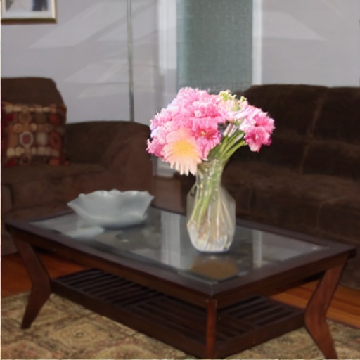
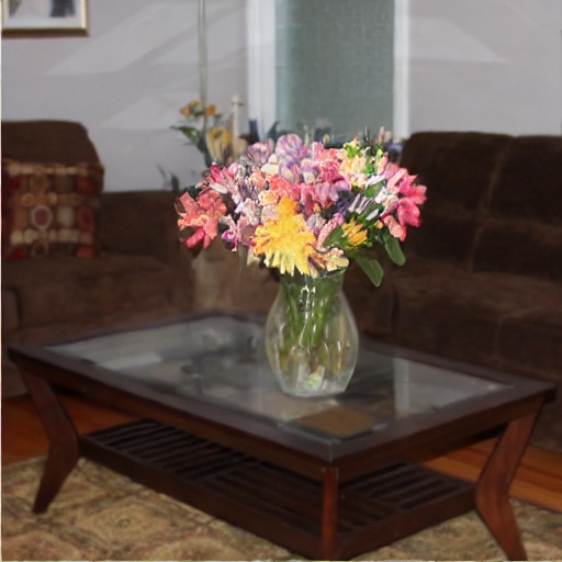
Stable Diffusion
ADIR
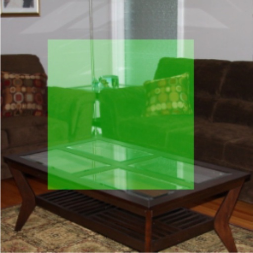
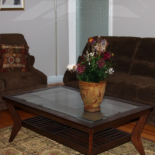
“A vase of flowers on the table of a living room”
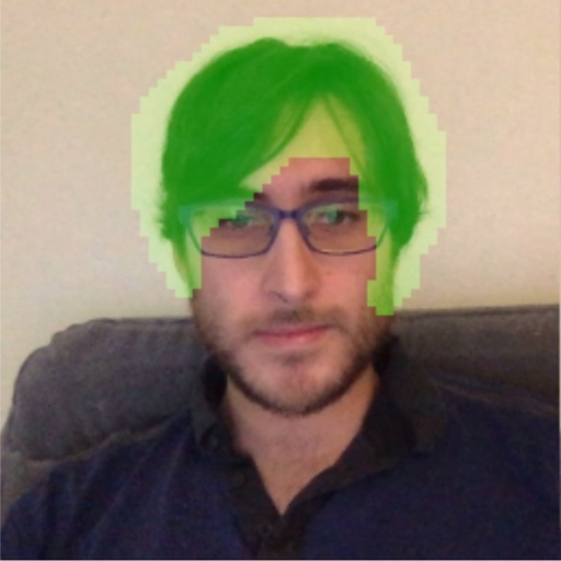
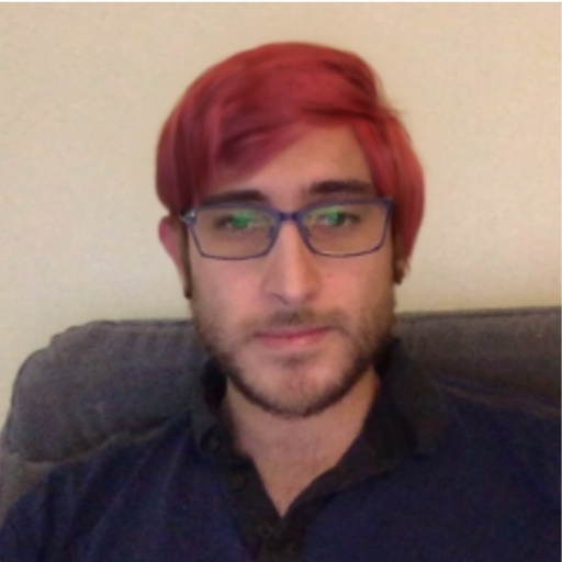
“A man with red hair”
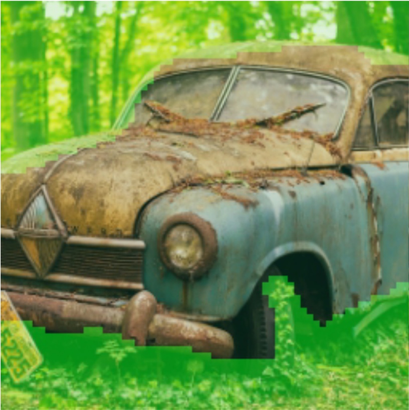
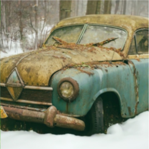
“An old car in a snowy forest”


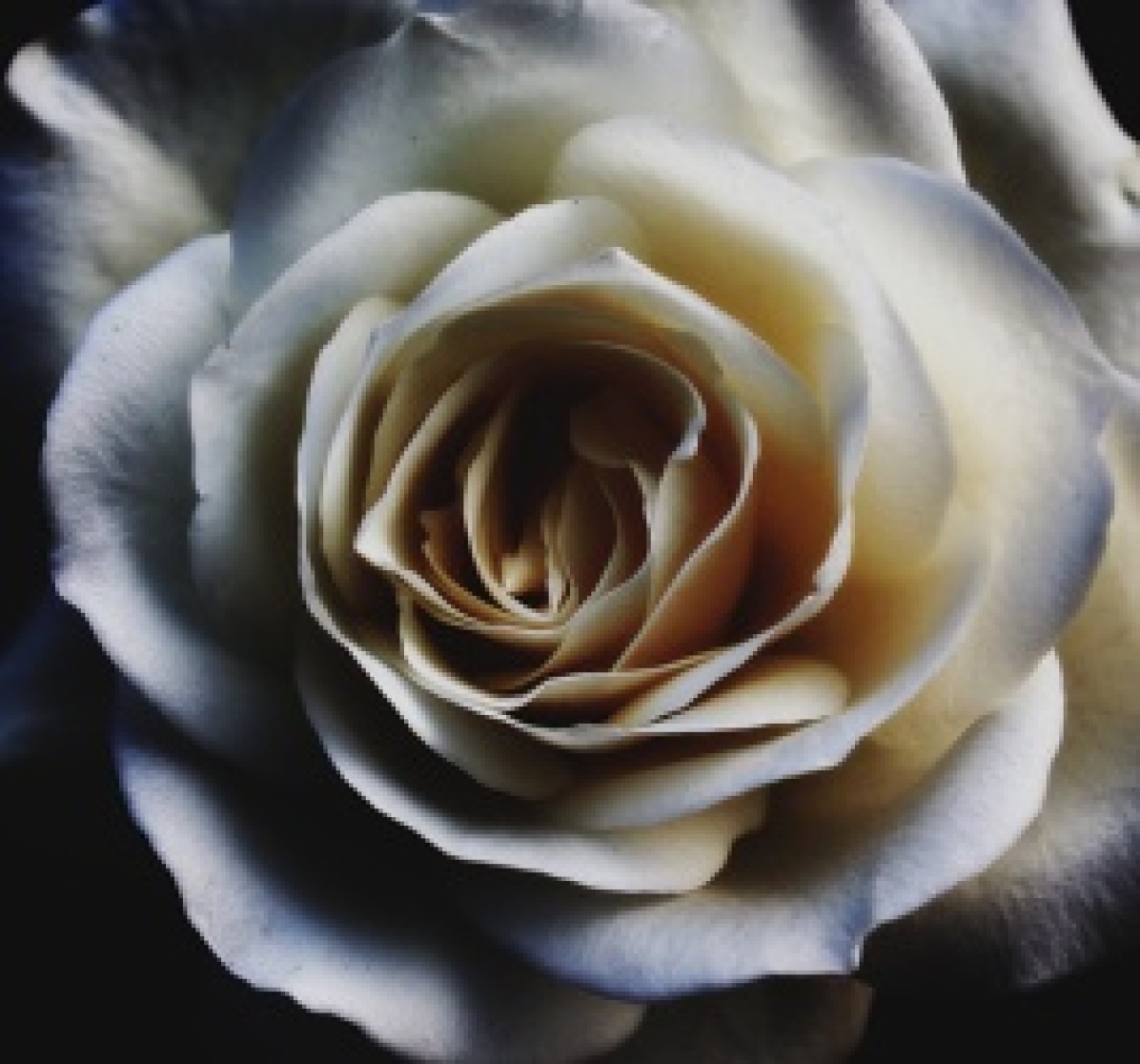
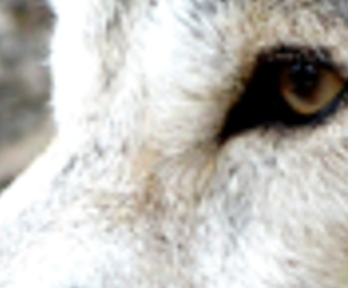
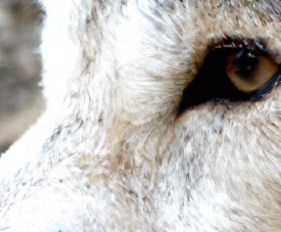
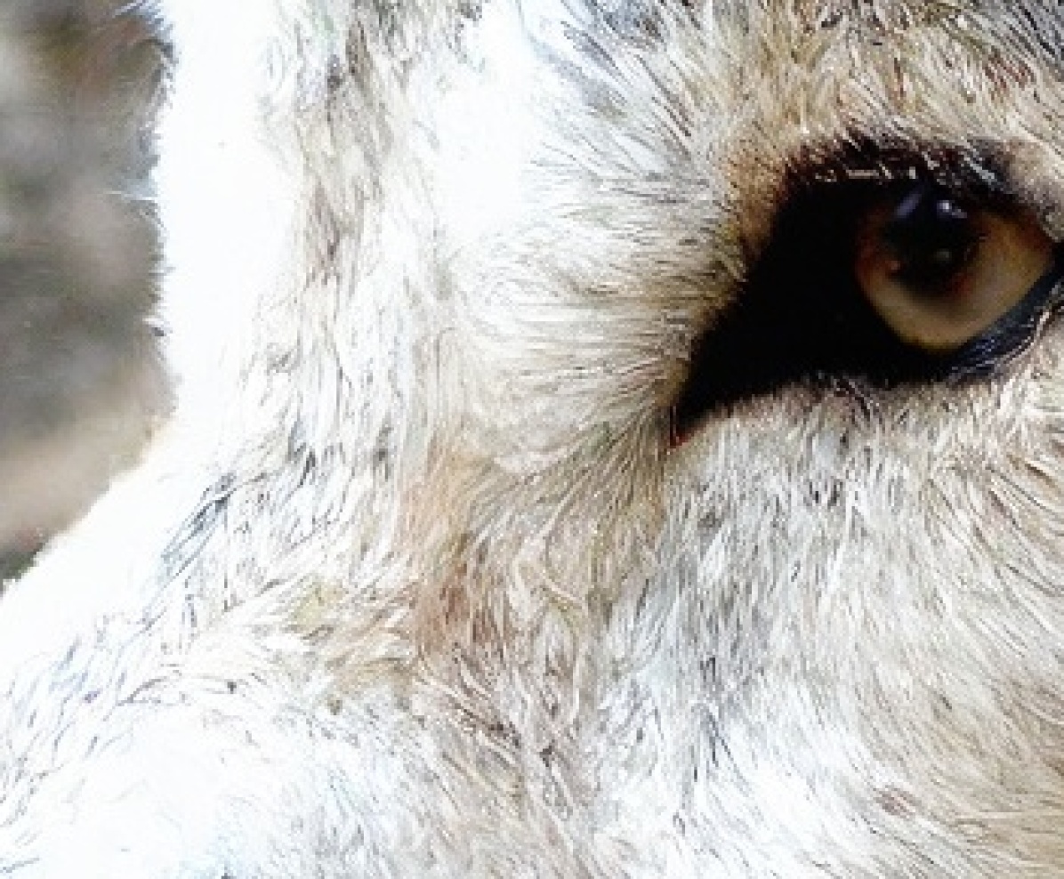
0ptGround Truth
![[Uncaptioned image]](/html/2212.03221/assets/x1.jpg)
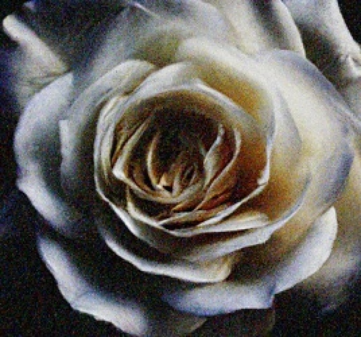
0ptBicubic 8![[Uncaptioned image]](/html/2212.03221/assets/x2.jpg) 0ptGuided Diffusion [13]
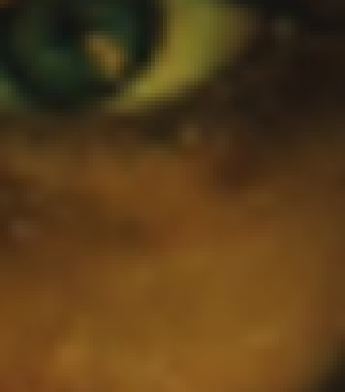
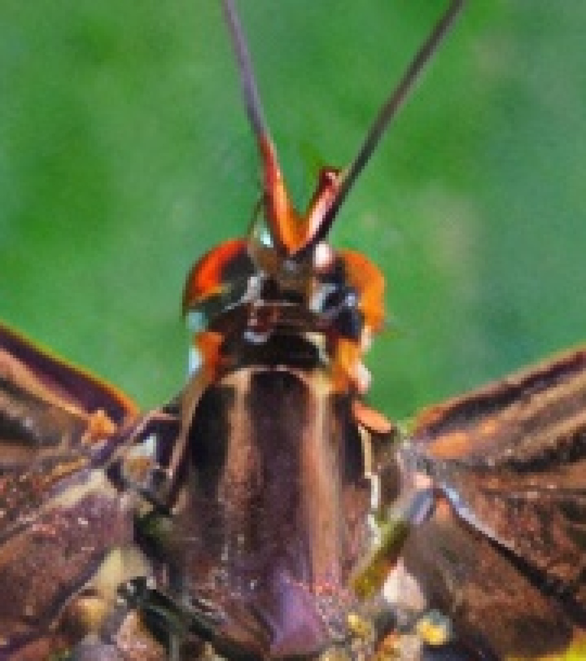
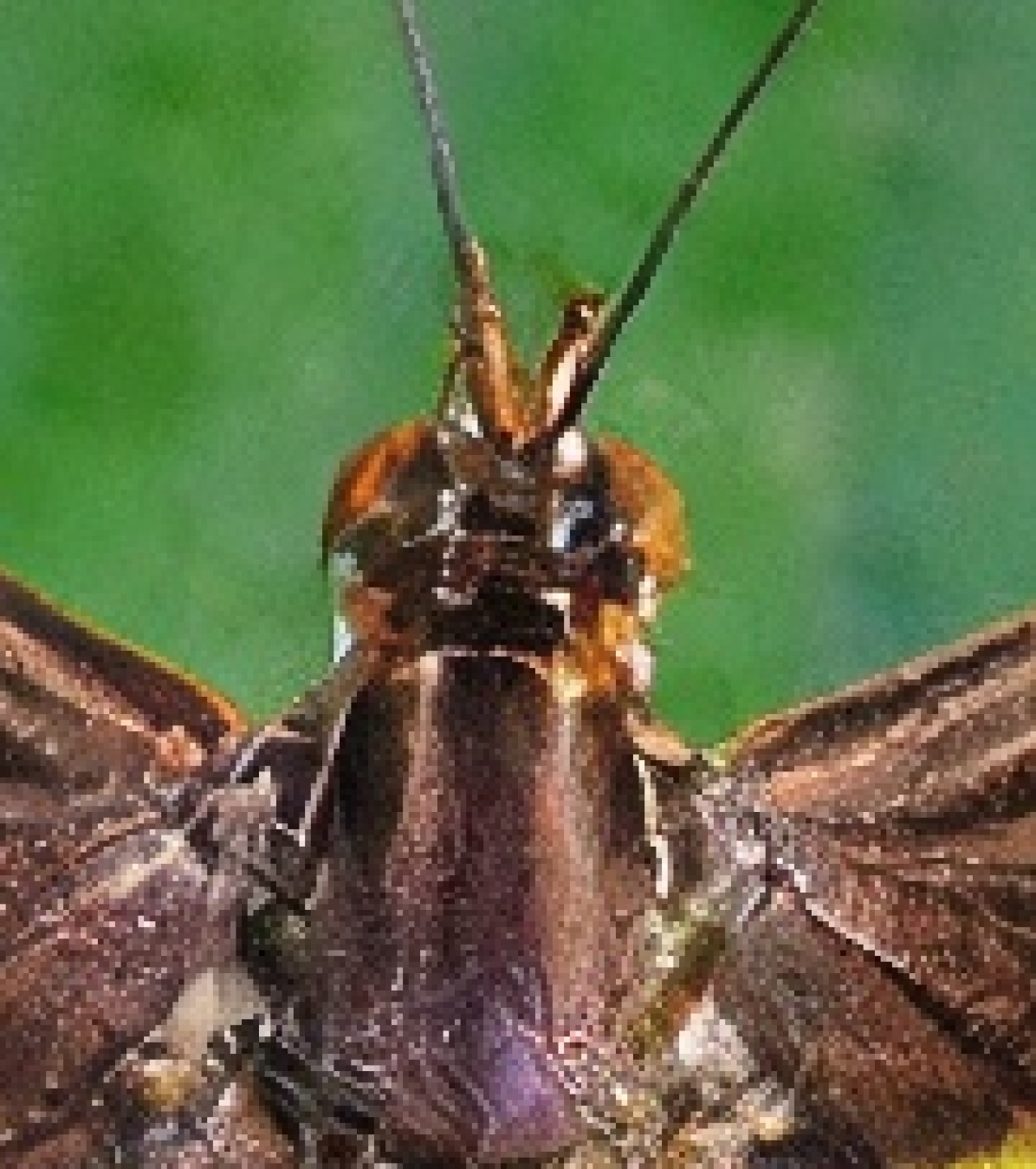
0ptGuided Diffusion [13]
![[Uncaptioned image]](/html/2212.03221/assets/x3.jpg)
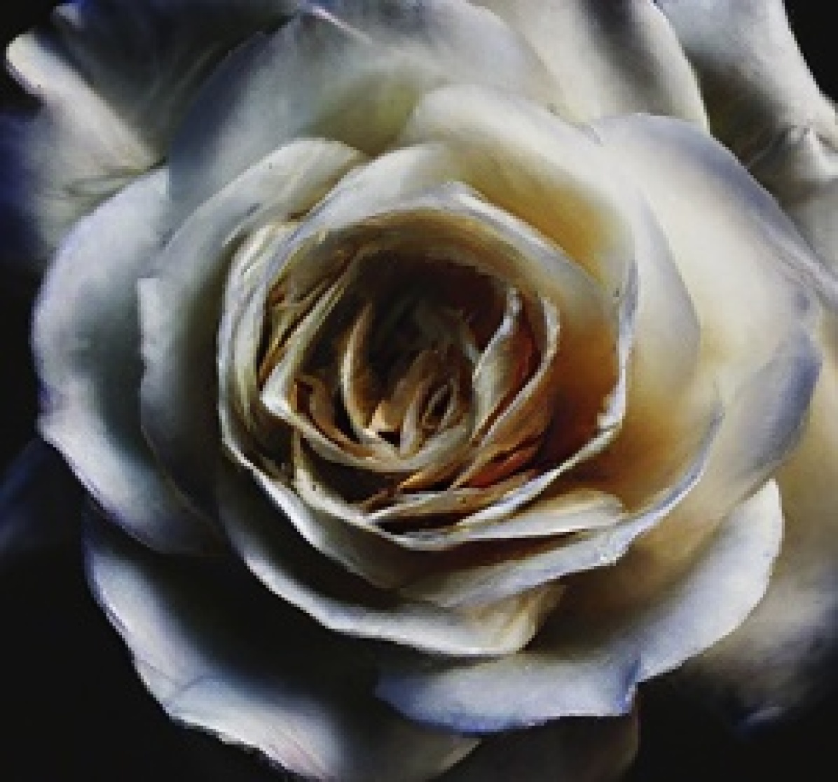
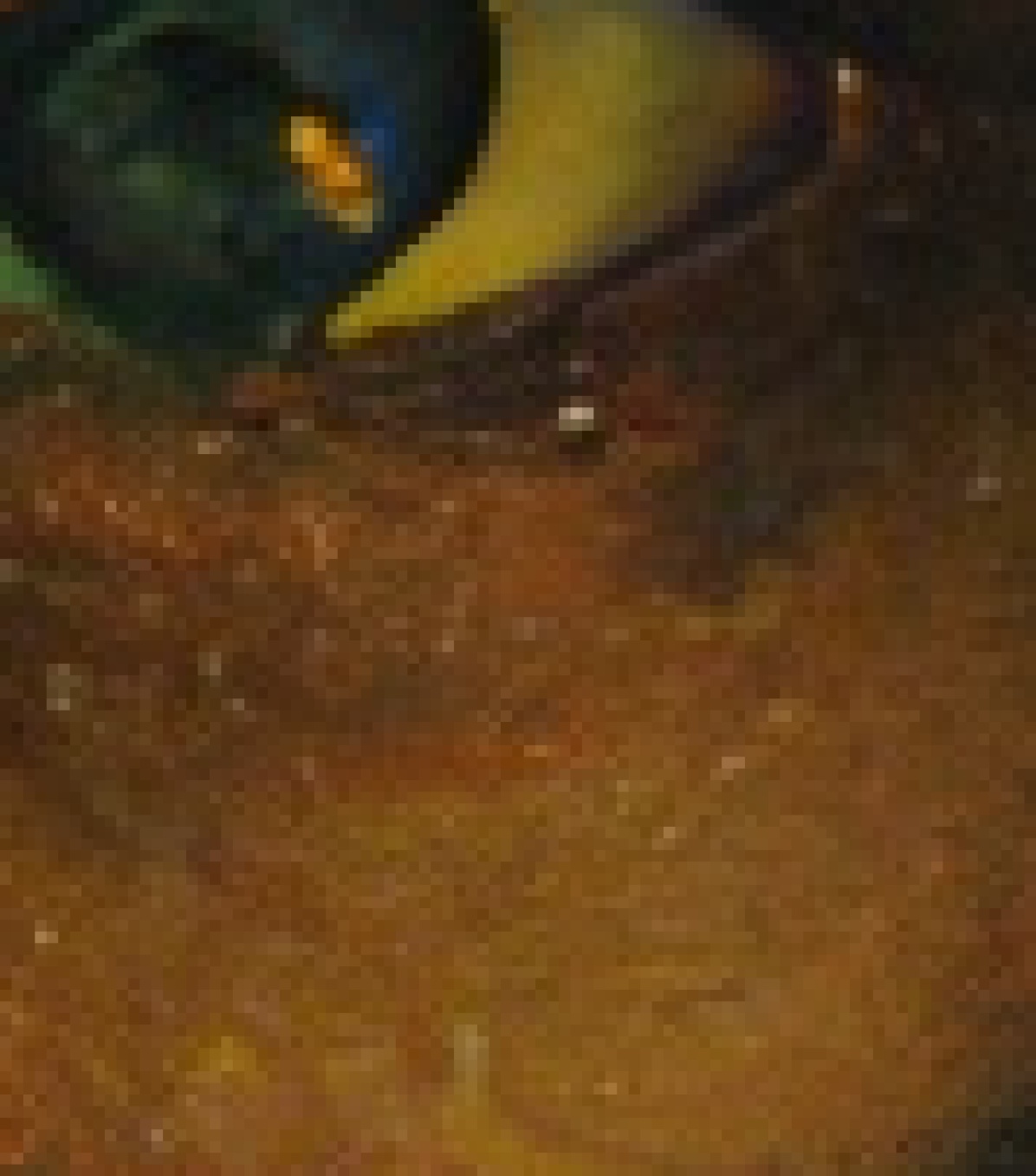
0ptADIR (ours)![[Uncaptioned image]](/html/2212.03221/assets/x4.jpg) 0ptGround Truth
0ptGround Truth
0ptBicubic 4
0ptStable Diffusion [36]
0ptADIR (ours)
1 Introduction
Image reconstruction problems appear in a wide range of applications, where one would like to reconstruct an unknown clean image from its degraded version , which can be noisy, blurry, low-resolution, etc. The acquisition (forward) model of in many important degradation settings can be formulated using the following linear model
| (1) |
where is the measurement operator (blurring, masking, sub-sampling, etc.) and is the measurement noise. Typically, just fitting the observation model is not sufficient for recovering successfully. Thus, prior knowledge on the characteristics of is needed.
Over the past decade, many works suggested solving the inverse problem in Eq. (1) using a single execution of a deep neural network, which has been trained on pairs of clean images and their degraded versions obtained by applying the forward model (1) on [14, 45, 28, 51]. Yet, these approaches tend to overfit the observation model and perform poorly on setups that have not been considered in training [41, 47, 20]. Tackling this limitation with dedicated training for each application is not only computationally inefficient but also often impractical. This is because the exact observation model may not be known before inference time.
Several alternative approaches such as Deep Image Prior [48], zero-shot-super-resolution [41] or GSURE-based test-time optimization [1] rely solely on the observation image . They utilize the implicit bias of deep neural networks and gradient-based optimizers, as well as the self-recurrence of patterns in natural images when training a neural model directly on the observation and in this way reconstruct the original image. Although these methods are not limited to a family of observation models, they usually perform worse than data-driven methods, since they do not exploit the robust prior information that the unknown image share with external data that may contain images of the same kind. Other popular approaches, which do exploit external data while remaining flexible to the observation model, use deep models for imposing only the prior. Such methods typically use pretrained deep denoisers [52, 3, 46, 50] or generative adversarial networks (GANs) [8, 12, 21] within their optimization schemes, where consistency of the reconstruction with the observation is maintained by minimizing a data-fidelity term.
Recently, diffusion models [13, 31, 42, 18] have shown remarkable capabilities in generating high-fidelity images. These models are based on constructing a Markov chain diffusion process of length for each training sample. In addition, they learn the reverse process, namely, the denoising operation between each two points in the chain. Sampling images via pretrained diffusion models is performed by starting with a pure white Gaussian noise image, This is followed by progressively sampling a less noisy image, given the previous one, until reaching a clean image after iterations. Since diffusion models capture prior knowledge of the data, one may utilize them as deep priors/regularization for inverse problems of the form (1) [44, 29, 5, 22, 9, 36].
In this work, we propose an Adaptive Diffusion framework for Image Reconstruction (ADIR). First, we devise a diffusion guidance sampling scheme that solves (1) while restricting the reconstruction of to the range of a pretrained diffusion model. Our scheme is based on novel modifications to the guidance used in [13] (see Section 3.2 for details). Then, we propose two techniques that use the observations to adapt the diffusion network to patterns beneficial for recovering the unknown . Adapting the model’s parameters is based either directly on or on external images similar to in some neural embedding space that is not sensitive to the degradation of . These images may be retrieved from a diverse dataset and the embedding can be calculated using an off-the-shelf encoder model for images such as CLIP [34]. As far as we know, our ADIR framework is the first adaptive diffusion approach for inverse problems. We evaluate it with two state-of-the-art diffusion models: Stable Diffusion [36] and Guided Diffusion [13], and show that it outperforms existing methods in the super-resolution and deblurring tasks. Finally, we demonstrate that our proposed adaptation strategy can be employed also for text-guided image editing.
2 Related Work
Diffusion models
In recent years, many works utilized diffusion models for image manipulation and reconstruction tasks [36, 23, 22, 49, 39], where a denoising network is trained to learn the prior distribution of the data. At test time, some conditioning mechanism is combined with the learned prior to solve very challenging imaging tasks [5, 4, 10].
In [49, 39] the problems of deblurring and super-resolution were considered. Then, a diffusion model has been trained to perform this task where instead of adding noise at each of its steps, a blur or downsampling is performed. In this way, the model learns to carry out the deblurring or super-resolution task directly. Notice that these models are trained for one specific task and cannot be used for the other as is.
The closest works to us are [16, 40, 23]. These very recent concurrent works consider the task of image editting and perform an adaptation of the used diffusion model using the provided input and external data. Yet, notice that neither of these works consider the task of image reconstruction as we do here or apply our proposed sampling scheme for this task.
Image-Adaptive Reconstruction
Adaptation of pretrained deep models, which serve as priors in inverse problems, to the unknown true through its observations at hand was proposed in [21, 47]. These works improve the reconstruction performance by fine-tuning the parameters of pretrained deep denoisers [47] and GANs [21] via the observed image instead of keeping them fixed during inference time. The image-adaptive GAN (IAGAN) approach [21] has led to many follow up works with different applications, e.g., [6, 33, 35, 32]. Recently, it has been shown that one may even fine-tune a masked-autoencoder to the input data at test-time for improving the adaptivity of classification neural networks to new domains [15].
In this paper we consider test-time adaptation of diffusion models for inverse problems. As far as we know, adaptation of diffusion models has not been proposed. Furthermore, while existing works fine-tune the deep priors directly using , we propose an improved strategy where the tuning is based on external images similar to that are automatically retrieved from an external dataset.
3 Method
We now turn to present our proposed approach. Yet, before doing that we first provide a short introduction to regular denoising diffusion models. After that we describe our proposed strategy for modifying the sampling scheme of diffusion models for the task of image reconstruction. Finally, we present our suggested adaptation scheme.
3.1 Denoising Diffusion Models
Denoising diffusion models [42, 18] are latent variable generative models, with latent variables (the same dimensionality as the data ). Given a training sample , these models are based on constructing a diffusion process (forward process) of the variables as a Markov chain from to of the form
| (2) |
where , and is the diffusion variance schedule (hyperparameters of the model). Note that sampling can be done via a simplified way using the parametrization [18]:
| (3) |
where and . The goal of these models is to learn the distribution of the reverse chain from to , which is parameterized as the Markov chain
| (4) |
where ,
| (5) |
and denotes all the learnable parameters. Essentially, is an estimator for the noise in (up to scaling).
The parameters of the diffusion model are optimized by minimizing evidence lower bound [42], a simplified score-matching loss [18, 43], or a combination of both [13, 31]. For example, the simplified loss involves the minimization of
| (6) |
in each training iteration, where is drawn from the training data, uniformly drawn from and the noise is drawn from .
Given a trained diffusion model , one may generate a sample from the learned data distribution by initializing and running the reverse diffusion process by sampling
| (7) |
where and is defined in (5).
The class-guided sampling method that has been proposed in [13] modifies the sampling procedure in (7) by adding to the mean of the Gaussian a term that depends on the gradient of an offline-trained classifier, which has been trained using noisy images for each , and approximates the likelihood , where is the desired class. This procedure has been shown to improve the quality of the samples generated for the learned classes.
3.2 Diffusion based Image Reconstruction
We turn now to extend the guidance method of [13] to image reconstruction. First, we conceptually generalize their framework to inverse problems of the form (1). Namely, given the observed image , we modify the guided reverse diffusion process to generate possible reconstructions of that are associated with rather than arbitrary samples of a certain class. Similarly to [13], ideally, the guiding direction at the iteration should follow from (the gradient of) the likelihood function .
The key difference between our framework and [13] is that we need to base our method on the specific degraded image rather than on a classifier that has been trained for each level of noise of . However, only the likelihood function is known, i.e., of the clean image that is available only at the end of the procedure, and not for every . To overcome this issue, we propose a surrogate for the intermediate likelihood functions . Our relaxation resembles the one in a recent concurrent work [11]. Yet, their sampling scheme is significantly different and has no adaptation ingredient.
Similar to [13], we guide the diffusion progression using the log-likelihood gradient. Formally, we are interested in sampling from the posterior
| (8) |
where is the distribution of conditioned on , and is the learned diffusion prior. For brevity, we omit the arguments of and in the rest of this subsection.
Under the assumption that the likelihood has low curvature compared to [13], the following approximation using Taylor expansion around is valid
| (9) |
where , and is a constant that does not depend on . Then, similar to the computation in [13], we can use (9) to express the posterior (8) in the following form
| (10) |
where , and is some constant that does not depend on . Therefore, for conditioning the diffusion reverse process on , one needs to evaluate the derivative from a (different) log-likelihood function at each iteration .
Observe that we know the exact log-likelihood function for . Since the noise in (1) is white Gaussian with variance , we therefore have following distribution
| (11) |
In the denoising diffusion setup, is related to using the observation model (1). Therefore,
| (12) |
However, we do not have tractable expressions for the likelihood functions . Therefore, motivated by the expression above, we propose the following approximation
| (13) |
where
| (14) |
is an estimation of from , which is based on the (stochastic) relation of and in (3) and the random noise is replaced by its estimation .
From (11) and (13) it follows that in (9) can be approximated at each iteration by evaluating (e.g., via automatic-differentiation)
| (15) |
Note that existing methods [11, 22, 44] either use a term that resembles (15) with the naive approximation [22, 44], or significantly modify (15) before computing it via automatic derivation framework [11] (we observed that trying to compute the exact (15) is unstable due to numerical issues). For example, in the official implementation of [11], which uses automatic derivation, the squaring of the norm in (15) is dropped even though this is not stated in their paper (otherwise, the reconstruction suffers from significant artifacts). In our case, we use the following relaxation to overcome the stability issue of using (15) directly. For a pretrained denoiser predicting from and we have
| (16) |
where . Consequently, we propose to replace the expression for (the guiding likelihood direction at each iteration ) that is given in (15) with a surrogate obtained by evaluating the derivative of (16) w.r.t. , which is given by
| (17) |
that can be used for sampling the posterior distribution as detailed in Algorithm 1.
3.3 Adaptive Diffusion
Having defined the guided inverse diffusion flow for image reconstruction, we turn to discuss how one may adapt a given diffusion model to a given degraded image as defined in (1). Assume we have a pretrained diffusion model , then the adaptation scheme is defined by the following minimization problem
| (18) |
which can be solved efficiently using stochastic gradient descent, where at each iteration the gradient step is performed on a single term of the sum above, for chosen randomly.
Adapting the denoising network to the measurement image , allows it to learn cross-scale features recurring in the image. Such an approach has been proven to be very helpful in reconstruction-based algorithms as shown in [21, 47].
However, in some cases where the image does not satisfy the assumption of recurring patterns across scales, this approach can lose some of the sharpness captured in training. Therefore, in this work we extend the approach to few-shot fine-tuning adaptation, where instead of solving (18) w.r.t. , we propose an algorithm for retrieving images similar to from a large dataset of diverse images, using off-the-shelf embedding distance.
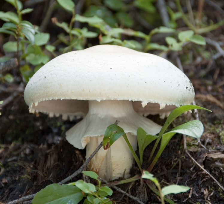
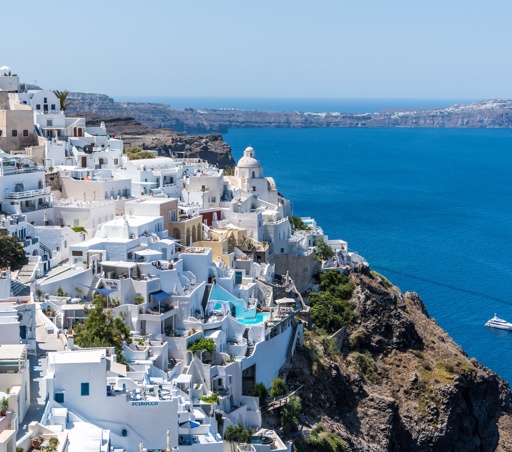
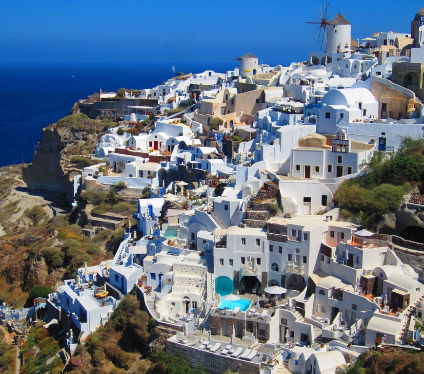
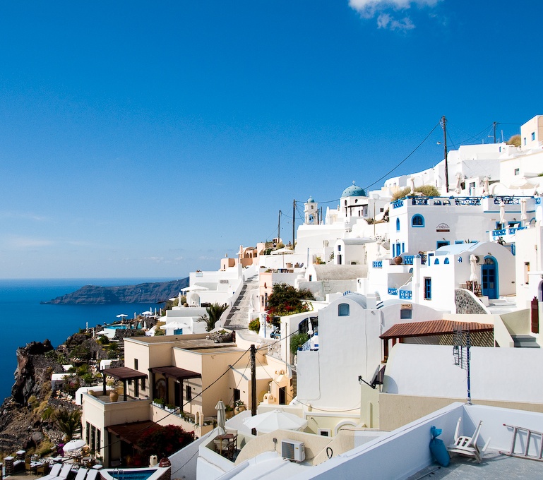
Let be some off-the-shelf multi-modal encoder trained on visual-language modalities. Examples include CLIP [34], BLIP [27], and CyCLIP [17]). Let and be the visual and language encoders respectively. Then, given a large diverse dataset of natural images, we propose to retrieve images, denoted by , with minimal embedding distance from . Formally, let be an arbitrary external dataset, then
| (19) |
where is the spherical distance and can be either the visual or language encoder depending on the provided conditioning of the application.
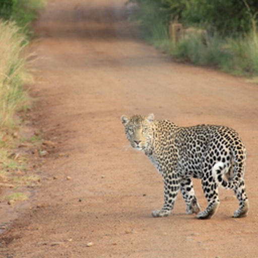
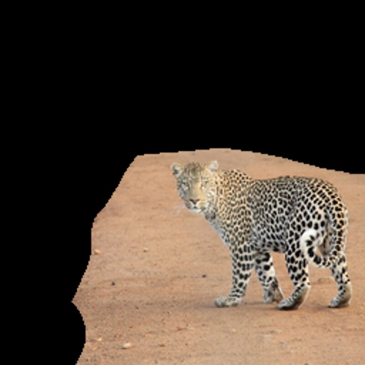
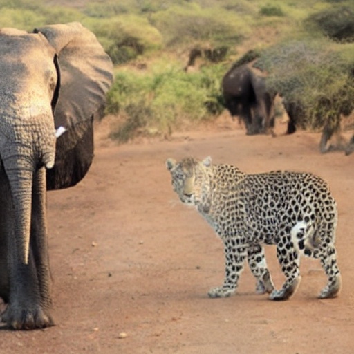
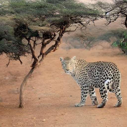
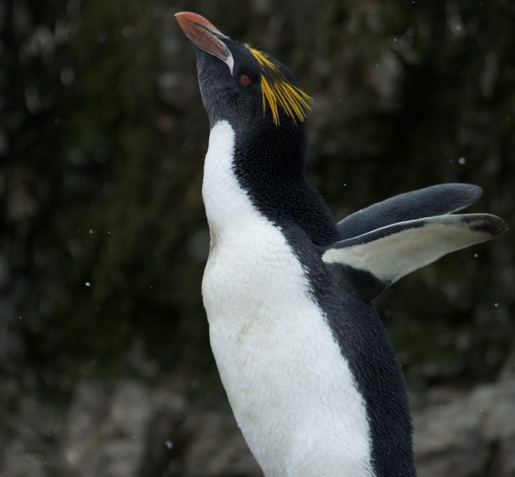
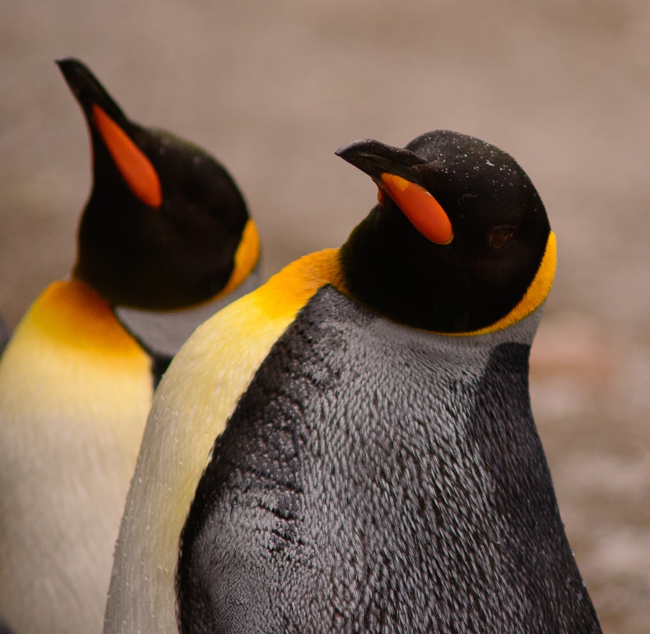
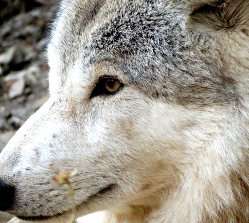
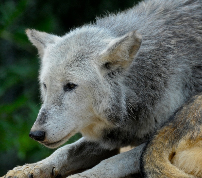
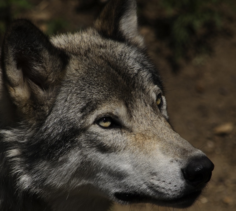
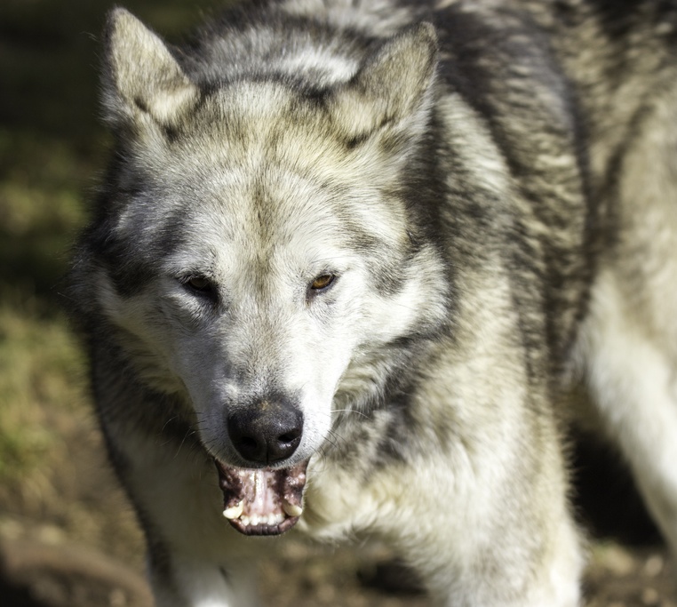
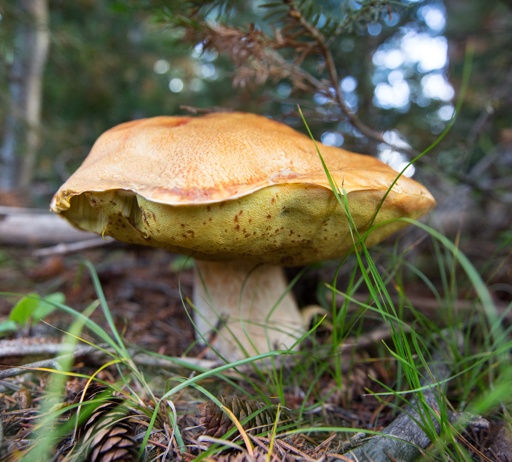
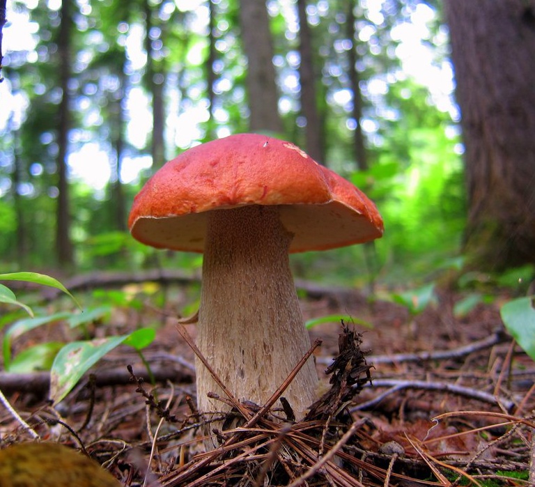
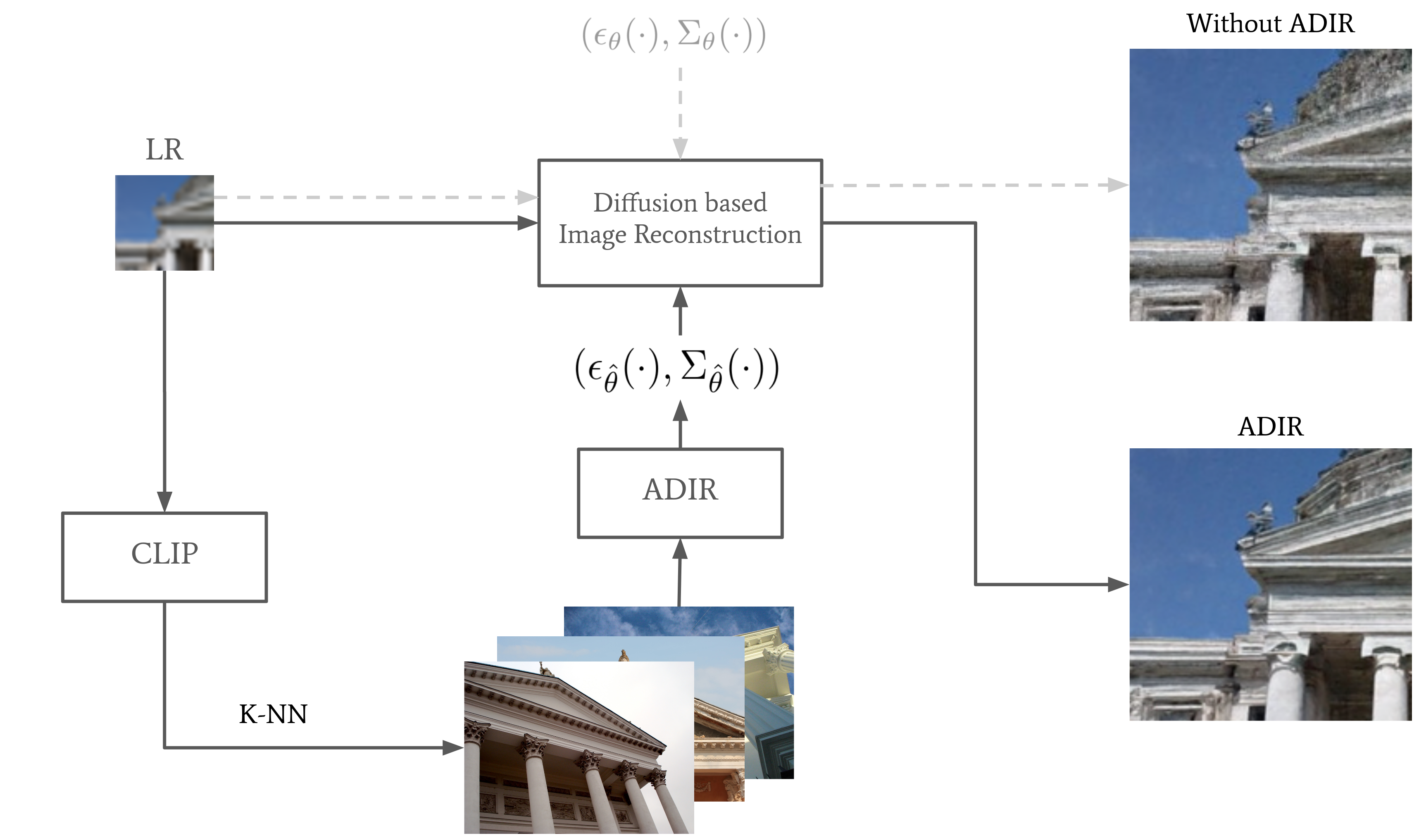
After retrieving -NN images from , we fine-tuning the diffusion model on them, which adapts the denoising network to the context of , where we use the loss in (6) to modify the denoiser parameters . We refer to this K-NN based adaptation technique as ADIR (Adaptive Diffusion for Image Reconstruction), which is described schematically in Figure 1.


4 Experiments
We evaluate our method on two state-of-the-art diffusion models, Guided Diffusion (GD) [13] and Stable Diffusion (SD) [36], showing results on super-resolution and deblurring. In addition, we show how the adaptive diffusion can be used for the task of text-based editing using stable diffusion. In the project web page we provide more comparisons and setups.
Guided diffusion [13] provides several models with a conditioning mechanism built-in the denoiser. However, in our case, we perform the conditioning using the -likelihood term. Therefore, we used the unconditional model that was trained on ImageNet [37] and produces images of size . In the original work, the conditioning for generating an image from an arbitrary class was performed using a classifier trained to classify the noisy sample directly, where the log-likelihood derivative can be obtained by deriving the corresponding logits w.r.t. directly. In our setup, the conditioning is performed using in (17), where is defined by the reconstruction task, which we specify in the sequel.
In addition to GD, we demonstrate the improvement that can be achieved using stable diffusion [36], where we use the publicly available super-resolution and text-based editing models for it. Instead of training the denoiser on the natural images domain directly, they suggest to use a Variational Auto Encoder (VAE) and train the denoiser using a latent representation of the data. Note that the lower dimensionality of the latent enables the network to be trained on higher resolutions.
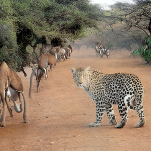
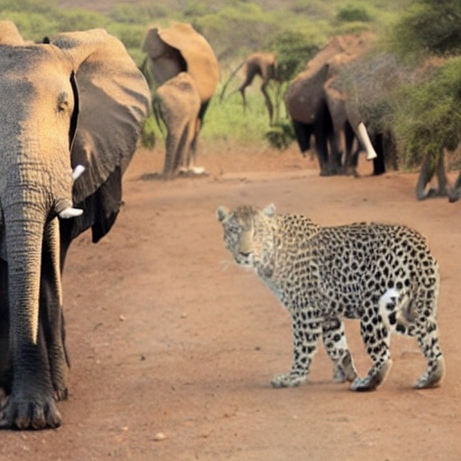
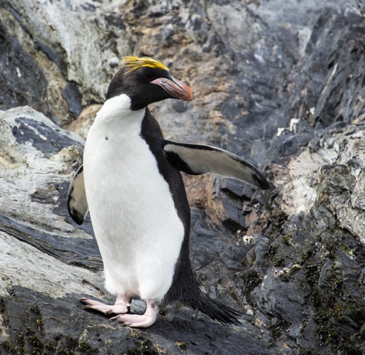
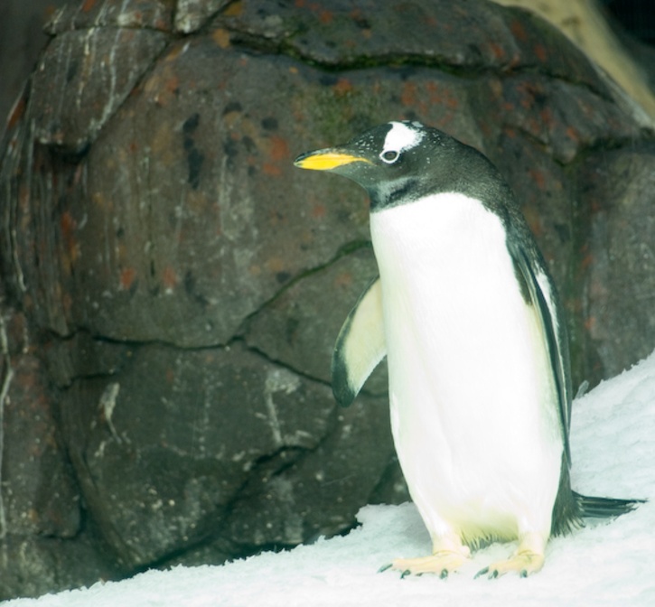
In all cases, we adapt the diffusion models in the image adaptive scheme presented in section 3.3, using the Google Open Dataset [26] as the external dataset , from which we retrieve images, where for GD and for SD (several examples of retrieved images are shown in Figure 6). For optimizing the network parameters we use Adam [25] and stabilize the training using Exponential Moving Average (EMA). The specific implementation configurations are detailed in Table 4. We run all of our experiments on a NVIDIA RTX A6000 48GB card, which allows us to fine-tune the models by randomly sampling a batch of 6 images from , where in each iterations we use the same for images in the batch.
| Bicubic | Guided Diffusion | IA | ADIR (GD) | |
|---|---|---|---|---|
| SRx4 | 29.847 / 3.617 | 64.630 / 4.876 | 63.973/4.807 | 68.756 / 5.163 |
| SRx8 | 17.915 / 3.523 | 54.406 / 4.433 | - | 58.580 / 4.476 |
| Bicubic | Stable Diffusion | ADIR (SD) | |
|---|---|---|---|
| SRx4 | 36.953 / 4.159 | 69.184 / 5.073 | 72.703 / 5.545 |
| Guided Diffusion | ADIR (GD) | |
|---|---|---|
| Uniform Deblur () | 49.195 / 4.196 | 56.874 / 4.403 |
| Uniform Deblur () | 58.665 / 4.812 | 61.655 / 4.880 |
| Gaussian deblur (256) | 48.114 / 4.013 | 51.804 / 4.194 |
4.1 Super Resolution
In the Super-Resolution (SR) task one would like to reconstruct a high resolution image from its low resolution image , where in this case represents an anti-aliasing filter followed by sub-sampling with stride , which we refer to as the scaling factor. In our use-case we employ a bicubic anti-aliasing filter and assume , similarly to most SR works.
Here we apply our approach on two different diffusion based SR methods, Stable Diffusion [36], and section 3.2 approach combined with the unconditional diffusion model from [13]. In Stable Diffusion, the low-resolution image is upscaled from to , while in Guided Diffusion we use the unconditional model trained on images, to upscale from to resolution. When adapting Stable diffusion, we downsample random crops of the -NN images using , which we encode using the VAE and plug into the network conditioning mechanism. We fine-tune both models using random crops of the -NN images, to which we then add noise using the scheduler provided by each model.
The perception preference of generative models-based image reconstruction has been seen in many works [21, 8, 7]. Therefore, we chose a perception-based measure to evaluate the performance of our method. Specifically, we use the state-of-the-art AVA-MUSIQ and KonIQ-MUSIQ perceptual quality assessment measures [24], which are state-of-the-art image quality assessment measures. We report our results using the two measures averaged on the first 50 validation images of the DIV2K [2] dataset. As can be seen in Tables 1, 2, our method significantly outperforms both Stable Diffusion and GD-based reconstruction approaches. We compare our SR results to Stable Diffusion SR and Guided Diffusion without adaptation, as well as using Image Adaptation (IA) performed on with no external data. The latter is done only for guided diffusion and show inferior performance compared to using external data. Therefore, in the other experiments we use only the external data for improving the optimization. A clear dominance of our method can be seen in the tables.
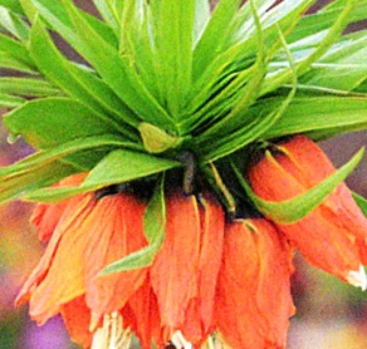
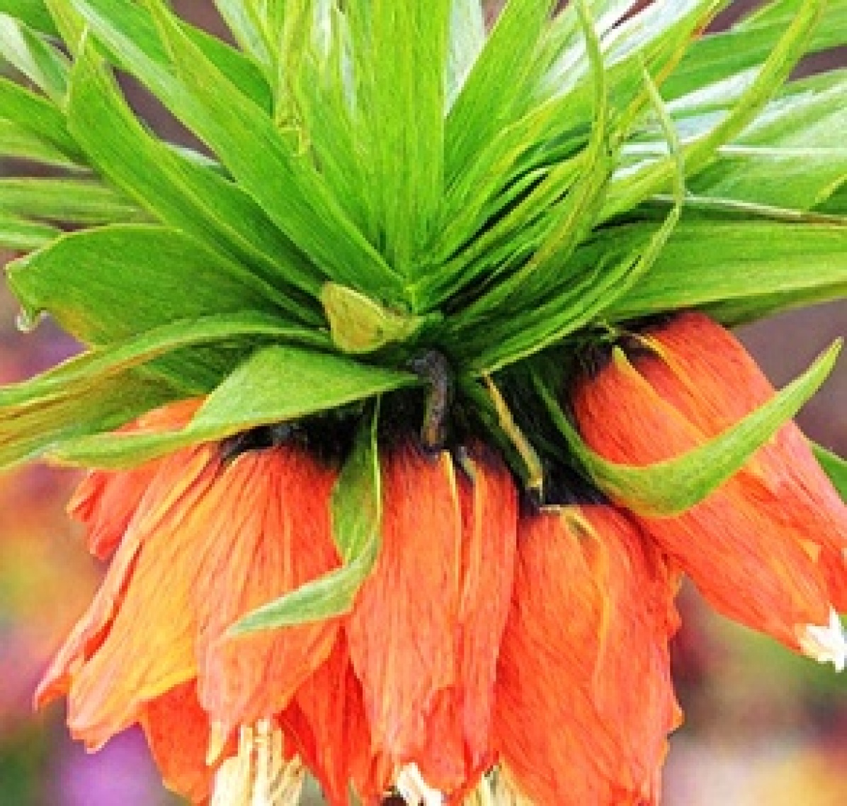
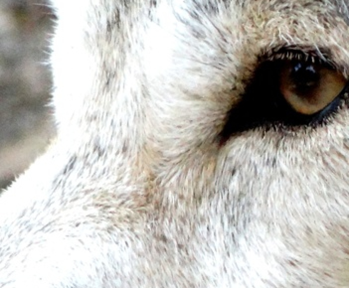
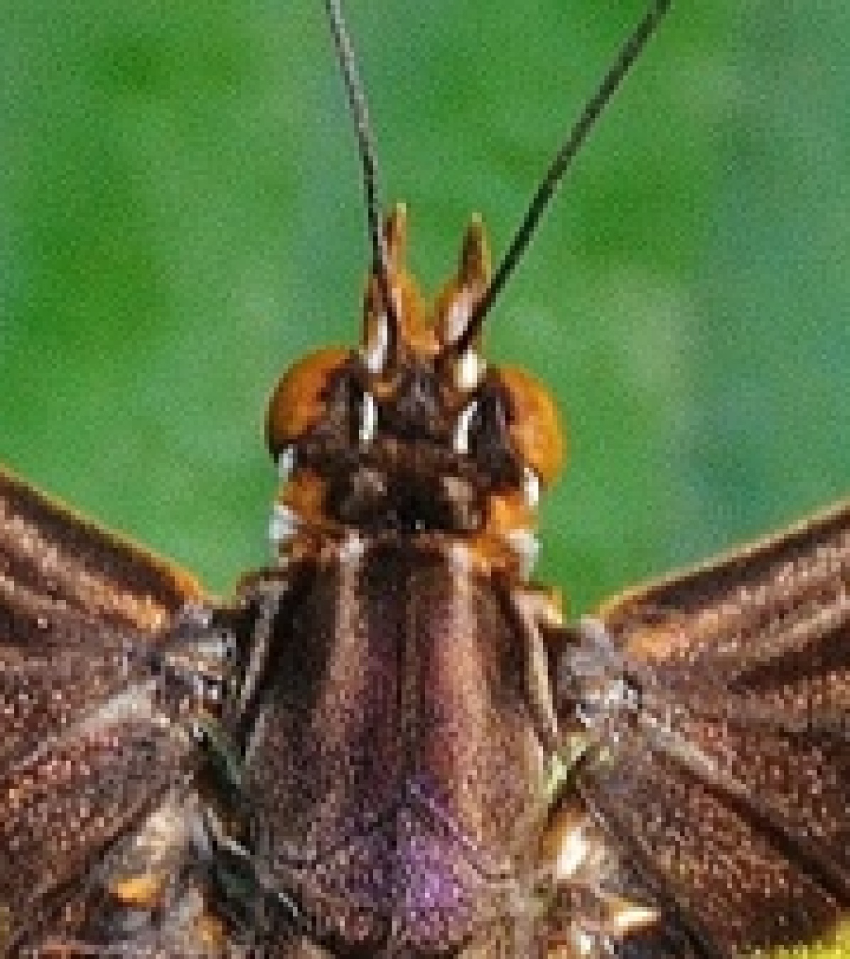
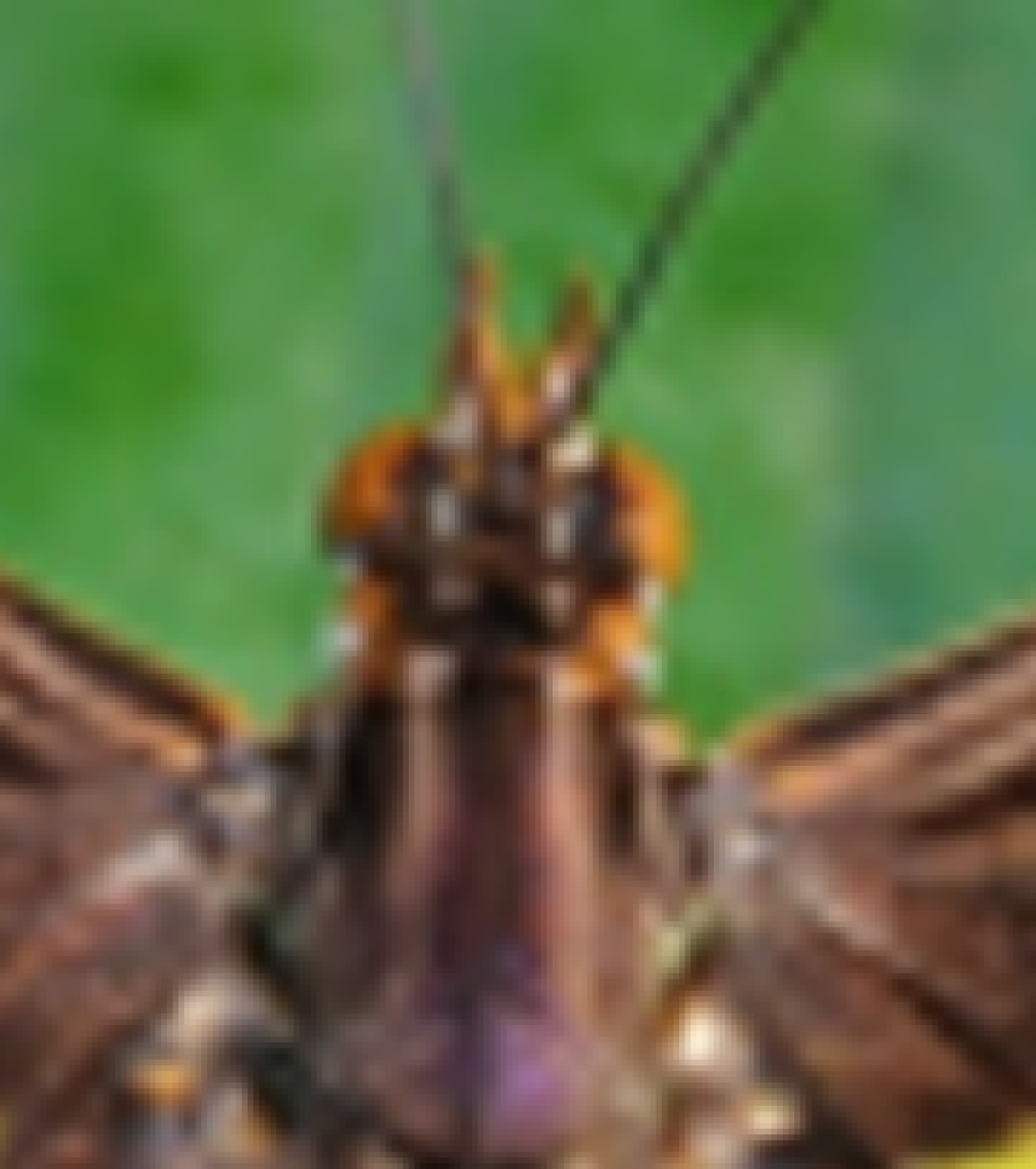
We also show qualitative results in Figures ‣ 0 Super-resolution with scale factors 4 and 8, using Stable Diffusion and Guided Diffusion, and our method ADIR. The adaptability of ADIR allows reconstructing finer details. and 3. As can be seen, our method achieves superior restoration quality, where in some cases it restores fine details that were blurred out in the acquisition of the ground-truth image.
4.2 Deblurring
In deblurring, is obtained by applying a uniform blur filter of size on , followed by adding measurment noise , which in our setting is .
We apply the approach in section 3.2 on Guided Diffusion unconditional model [13] to solve the task. In this case, can be implemented by applying the blur kernel on a given image.
We use the unconditional diffusion model provided by GD [13], which was trained on size images. Yet, in our tests, we solve the deblurring task on images of size as well as , which emphasizes the remarkable benefit of the adaptation, as it allows the model to generalize to resolutions not seen in training.
Similar to SR, in Table 3 we report the KonIQ-MUSIQ and AVA-MUSIQ [24] measures, averaged on the first 50 DIV2K validation images [2], where we compare our approach to the guided diffusion reconstruction without image adaptation. A visual comparisons are also available in Figure 2, where a very significant improvement can be seen in both robustness to noise and reconstructing details.
4.3 Text-Guided Editing
Text-guided image editing is the task of completing a masked region of according to a prompt provided by the user. In this case, the diffusion model needs predict objects and textures correspondent to the provided prompt, therefore we chose to adapt the network on retrieved using the text encoder, i.e. by solving (19) using . For evaluating our method on this application, we use the state-of-the-art inpainting model of Stable Diffusion [36]. Where encoded and concatenated with the mask resized to latent dimension, which are then plugged to the denoising network. When adapting the network, we follow the training scheme of Stable Diffusion, where we use random masks and the classifier-free conditioning approach [19] used for training Stable Diffusion, where the text embedding is randomly chosen to either be the encoded prompt or the embedding of an empty prompt. Notice that we cannot compare to [16, 40, 23] as there is no code available for them. For some of them, we do not even have access to the diffusion model that they adapt [38]
Figure 5 presents the editing results and compares to both stable diffusion and GLIDE. GLIDE is the basis of the popular DALL-E-2 model. The images of GLIDE are taken from the paper. We use ADIR with stable diffusion and optimize them using the same seed.
Since Stable Diffusion was trained using a lossy latent representation with smaller dimensionality than the data, it is clear that GLIDE can achieve better results. However, because our method adapts the network to a specific scenario, it enables the model to produce cleaner and more accurate generations, as can be seen in Figure 5. In the first image we see that Stable Diffusion adds an object that does not blend well and has artifacts, while when combined with our approach the quality improves significantly. Similarly, in the second image we see that Stable Diffusion produces an inaccurate edit, where it adds a brown hair instead of red hair. This is again improved by our adaptation method.
5 Conclusion
We have presented the Adaptive Diffusion Image Reconstruction (ADIR) method, in which we improve the reconstruction results in several imaging tasks using off-the-shelf diffusion models. We have demonstrated how our adaptation can significantly improve existing state-of-the-art methods, e.g. Stable Diffusion for super resolution, where the exploitation of external data with the same context as , combined with our adaptation scheme leads to a significant improvement. Specifically, the produced images are sharper and have more details than the original ground truth image.
One limitation of our approach is that as is the case with all diffusion models, there is randomness in the generation results. Therefore, they quality of the output may depend on the seed used. Yet, we still find that when we compare our approach and the baseline with the same seed, we get an improvement in the vast majority of cases. We provide additional examples in the project web page of such randomly generated pairs with different random seeds to further show the consistent improvement that can be achieved by our proposed strategy.