Visual Query Tuning: Towards Effective Usage of Intermediate Representations for Parameter and Memory Efficient Transfer Learning

Abstract

Intermediate features of a pre-trained model have been shown informative for making accurate predictions on downstream tasks, even if the model backbone is kept frozen. The key challenge is how to utilize these intermediate features given their gigantic amount. We propose visual query tuning (VQT), a simple yet effective approach to aggregate intermediate features of Vision Transformers. Through introducing a handful of learnable “query” tokens to each layer, VQT leverages the inner workings of Transformers to “summarize” rich intermediate features of each layer, which can then be used to train the prediction heads of downstream tasks. As VQT keeps the intermediate features intact and only learns to combine them, it enjoys memory efficiency in training, compared to many other parameter-efficient fine-tuning approaches that learn to adapt features and need back-propagation through the entire backbone. This also suggests the complementary role between VQT and those approaches in transfer learning. Empirically, VQT consistently surpasses the state-of-the-art approach that utilizes intermediate features for transfer learning and outperforms full fine-tuning in many cases. Compared to parameter-efficient approaches that adapt features, VQT achieves much higher accuracy under memory constraints. Most importantly, VQT is compatible with these approaches to attain even higher accuracy, making it a simple add-on to further boost transfer learning. Code is available at https://github.com/andytu28/VQT.

1 Introduction

Transfer learning by adapting large pre-trained models to downstream tasks has been a de facto standard for competitive performance, especially when downstream tasks have limited data [59, 37]. Generally speaking, there are two ways to adapt a pre-trained model [27, 15]: updating the model backbone for new feature embeddings (the output of the penultimate layer) or recombining the existing feature embeddings, which correspond to the two prevalent approaches, fine-tuning and linear probing, respectively. Fine-tuning, or more specifically, full fine-tuning, updates all the model parameters end-to-end based on the new dataset. Although fine-tuning consistently outperforms linear probing on various tasks [54], it requires running gradient descent for all parameters and storing a separate fine-tuned model for each task, making it computationally expensive and parameter inefficient. These problems become more salient with Transformer-based models whose parameters grow exponentially [26, 17, 46]. Alternatively, linear probing only trains and stores new prediction heads to recombine features while keeping the backbone frozen. Despite its computational and parameter efficiency, linear probing is often less attractive due to its inferior performance.

Several recent works have attempted to overcome such a dilemma in transfer learning. One representative work is by Evci et al. [15], who attributed the success of fine-tuning to leveraging the “intermediate” features of pre-trained models and proposed to directly allow linear probing to access the intermediate features. Some other works also demonstrated the effectiveness of such an approach [14, 15]. Nevertheless, given numerous intermediate features in each layer, most of these methods require pooling to reduce the dimensionality, which likely would eliminate useful information before the prediction head can access it.

To better utilize intermediate features, we propose Visual Query Tuning (VQT), a simple yet effective approach to aggregate the intermediate features of Transformer-based models like Vision Transformers (ViT) [13]. A Transformer usually contains multiple Transformer layers, each starting with a Multi-head self-attention (MSA) module operating over the intermediate feature tokens (often $>100$ tokens) outputted by the previous layer. The MSA module transforms each feature token by querying all the other tokens, followed by a weighted combination of their features.

Taking such inner workings into account, VQT introduces a handful of learnable “query” tokens to each layer, which, through the MSA module, can then “summarize” the intermediate features of the previous layer to reduce the dimensionality. The output features of these query tokens after each layer can then be used by linear probing to make predictions. Compared to pooling which simply averages the features over tokens, VQT performs a weighted combination whose weights are adaptive, conditioned on the features and the learned query tokens, and is more likely to capture useful information for the downstream task.

At first glance, VQT may look superficially similar to Visual Prompt Tuning (VPT) [23], a recent transfer learning method that also introduces additional learnable tokens (i.e., prompts) to each layer of Transformers, but they are fundamentally different in two aspects. First, our VQT only uses the additional tokens to generate queries, not keys and values, for the MSA module. Thus, it does not change the intermediate features of a Transformer at all. In contrast, the additional tokens in VPT generate queries, keys, and values, and thus can be queried by other tokens and change their intermediate features. Second, and more importantly, while our VQT leverages the corresponding outputs of the additional tokens as summarized intermediate features, VPT in its Deep version disregards such output features entirely. In other words, these two methods take fundamentally different routes to approach transfer learning: VQT learns to leverage the existing intermediate features, while VPT aims to adapt the intermediate features. As will be demonstrated in section 4, these two routes have complementary strengths and can be compatible to further unleash the power of transfer learning. It is worth noting that most of the recent methods towards parameter-efficient transfer learning (PETL), such as Prefix Tuning [30] and AdaptFormer [10], all can be considered adapting the intermediate features [19]. Thus, the aforementioned complementary strengths still apply.

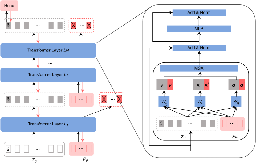
(a) VPT: Visual Prompt Tuning (deep version) [23]

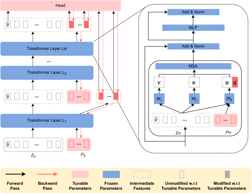
(b) Our VQT: Visual Query Tuning

Figure 1: Our Visual Query Tuning (VQT) vs. Visual Prompt Tuning (VPT) [23]. Our VQT allows linear probing to directly access the intermediate features of a frozen Transformer model for parameter-efficient transfer learning. The newly introduced query tokens in VQT (marked by the red empty boxes in the red shaded areas) only append additional columns (i.e., $\bm{Q}^{\prime}$) to the Query features $\bm{Q}$, not to the Value features $\bm{V}$ and the Key features $\bm{K}$. Thus, VQT keeps the intermediate features intact ( gray empty boxes), enabling it to bypass expensive back-propagation steps in training (hence memory efficient). In contrast, VPT modifies the intermediate features ( gray solid boxes) and needs more memory to learn its prompts. Please see section 3 for details.

Besides the difference in how to approach transfer learning, another difference between VQT and many other PETL methods, including VPT, is memory usage in training. While many of them freeze (most of) the backbone model and only learn to adjust or add some parameters, the fact that the intermediate features are updated implies the need of a full back-propagation throughout the backbone, which is memory-heavy. In contrast, VQT keeps all the intermediate features intact and only learns to combine them. Learning the query tokens thus bypasses many paths in the standard back-propagation, reducing the memory footprint by 76% compared to VPT.

We validate VQT on various downstream visual recognition tasks, using a pre-trained ViT [13] as the backbone. VQT surpasses the SOTA method that utilizes intermediate features [15] and full fine-tuning in most tasks. We further demonstrate the robust and mutually beneficial compatibility between VQT and existing PETL approaches using different pre-trained backbones, including self-supervised and image-language pre-training. Finally, VQT achieves much higher accuracy than other PETL methods in a low-memory regime, suggesting that it is a more memory-efficient method.

To sum up, our key contributions are

1. We propose VQT to aggregate intermediate features of Transformers for effective linear probing, featuring parameter and memory efficient transfer learning.

2. VQT is compatible with other PETL methods that adapt intermediate features, further boosting the performance.

3. VQT is robust to different pre-training setups, including self-supervised and image-language pre-training.

2 Related Work

Transformer. The splendent success of Transformer models [46] in natural language processing (NLP) [48] has sparked a growing interest in adopting these models in vision and multi-modal domains [26]. Since the proposal of the Vision Transformer (ViT) [13], Transformer-based methods have demonstrated impressive advances in various vision tasks, including image classification [35, 51, 44], image segmentation [49, 40], object detection [58, 7], video understanding [2, 36], point cloud processing [16, 56], and several other use cases [9, 50]. As Transformer models assume minimal prior knowledge about the structure of the problem, they are often pre-trained on large-scale datasets [11, 8, 39]. Given that the Transformer models are notably larger than their convolutional neural network counterparts, e.g., ViT-G (1843M parameters) [53] vs. ResNet-152 (58M parameters) [21], how to adapt the pre-trained Transformers to downstream tasks in a parameter and memory efficient way remains a crucial open problem.

PETL. The past few years have witnessed the huge success of parameter-efficient transfer learning (PETL) in NLP, aiming to adapt large pretrained language models (PLMs) to downstream tasks [25, 6]. Typically, PETL methods insert small learnable modules into PLMs and fine-tune these modules with downstream tasks while freezing the pretrained weights of PLMs [19, 29, 22, 38, 43, 5, 3, 47, 33, 41, 57]. The current dominance of Transformer models in the vision field has urged the development of PETL methods in ViT [23, 10, 24, 55, 34, 31]. Recently, Visual Prompt Tuning (VPT) [23] was proposed to prepend learnable prompts to the input embeddings of each Transformer layer. AdaptFormer [10] inserts a bottleneck-structured fully connected layers parallel to the MLP block in a Transformer layer. Convpass [24] inserts a convolutional bottleneck module while NOAH [55] performs a neural architecture search on existing PETL methods. Unlike all the aforementioned methods that update the output features of each Transformer layer, our VQT focuses on leveraging the frozen intermediate features. Thus, VQT is compatible with most existing PETL methods and enjoys memory efficiency.

Transfer learning with intermediate features. Intermediate features of a pre-trained model contain rich and valuable information, which can be leveraged in various tasks such as object detection [32, 4, 18] and OOD detection [28], etc. Recently, multiple works [12, 15, 14, 42] have demonstrated the effectiveness of these features on transfer learning. On the NLP side, LST [42] trains a lightweight Transformer network that takes intermediate features as input and generates output features for predictions. On the CV side, Evci et al. [15] attribute the success of fine-tuning to the ability to leverage intermediate features and proposed Head2Toe to select features from all layers for efficient transfer learning. Eom et al. [14] proposed utilizing intermediate features to facilitate transfer learning for multi-label classification. However, due to the massive number of intermediate features, most methods rely on the pooling operation to reduce the dimensionality, which may distort or eliminate useful information. This observation motivates us to introduce VQT, which learns to summarize intermediate features according to the downstream task.

3 Approach

We propose Visual Query Tuning (VQT) to adapt pre-trained Transformers to downstream tasks while keeping the backbone frozen. VQT keeps all the intermediate features intact and only learns to “summarize” them for linear probing by introducing learnable “query” tokens to each layer.

3.1 Preliminaries

3.1.1 Vision Transformer

Vision Transformers (ViT) [13] adapt the Transformer-based models [46] from NLP into visual tasks, by dividing an image $\bm{I}$ into a sequence of $N$ fixed-sized patches $\{\bm{I}^{(n)}\}_{n=1}^{N}$ and treating them as NLP tokens. Each patch $\bm{I}^{(n)}$ is first embedded into a $D$-dimensional vector ${\bm{x}}^{(n)}_{0}$ with positional encoding. The sequence of vectors is then prepended with a “CLS” vector ${\bm{x}}_{0}^{(\text{Class})}$ to generate the input $\bm{Z}_{0}=[{\bm{x}}_{0}^{(\text{Class})},{\bm{x}}^{(1)}_{0},\cdots,{\bm{x}}^{(N)}_{0}]\in\mathbb{R}^{D\times(1+N)}$ to the ViT. We use superscript/subscript to index token/layer.

Normally, a ViT has $M$ layers, denoted by $\{L_{m}\}_{m=1}^{M}$. Given the input $\bm{Z}_{0}$, the first layer $L_{1}$ generates the output $\bm{Z}_{1}=L_{1}(\bm{Z}_{0})=[{\bm{x}}_{1}^{(\text{Class})},{\bm{x}}^{(1)}_{1},\cdots,{\bm{x}}^{(N)}_{1}]\in\mathbb{R}^{D\times(N+1)}$, which is of the same size as $\bm{Z}_{0}$. That is, $\bm{Z}_{1}$ has $1+N$ feature tokens, and each corresponds to the same column in $\bm{Z}_{0}$. Such layer-wise processing then continues to generate the output of the next layer, $\bm{Z}_{m}=L_{m}(\bm{Z}_{m-1})$ for $m=2,\cdots,M$, taking the output of the previous layer as input. Finally, the “CLS” vector ${\bm{x}}_{M}^{(\text{Class})}$ in $\bm{Z}_{M}$ is used as the feature for prediction. Taking classification as an example, the predicted label $\hat{y}=\mathsf{Head}({\bm{x}}_{M}^{(\text{Class})})$ is generated by a linear classifier (i.e., a fully-connected layer).

Details of each Transformer layer. Our approach takes advantage of the inner workings of Transformer layers. In the following, we provide a concise background.

Each Transformer layer consists of a Multi-head Self-Attention (MSA) block, a Multi-Layer Perceptron (MLP) block, and several other operations including layer normalization and residual connections. Without loss of generality, let us consider a single-head self-attention block and disregard those additional operations.

Given the input $\bm{Z}_{m-1}$ to $L_{m}$, the self-attention block first projects it into three matrices, namely Query $\bm{Q}_{m}$, Key $\bm{K}_{m}$, and Value $\bm{V}_{m}$,

$$\bm{Q}_{m}=\bm{W}_{q}\bm{Z}_{m-1},\quad\bm{K}_{m}=\bm{W}_{k}\bm{Z}_{m-1},\quad\bm{V}_{m}=\bm{W}_{v}\bm{Z}_{m-1}.$$ (1)

Each of them has $1+N$ columns, corresponding to each column (i.e., token) in $\bm{Z}_{m-1}$. Then, the output of $L_{m}$, i.e., $\bm{Z}_{m}$, can be calculated by:

$$\bm{Z}_{m}=\mathsf{MLP}_{m}\circ\mathsf{MSA}_{m}(\bm{Z}_{m-1}),$$ (2)

$$\text{where}\hskip 5.0pt\mathsf{MSA}_{m}(\bm{Z}_{m-1})=\bm{V}_{m}\times\mathsf{Softmax}(\frac{\bm{K}_{m}^{\top}\bm{Q}_{m}}{\sqrt{D}}).$$ (3)

The $\mathsf{Softmax}$ is taken over elements of each column; the $\mathsf{MLP}_{m}$ is applied to each column of $\mathsf{MSA}_{m}(\bm{Z}_{m-1})$ independently.

3.1.2 Transfer Learning: Linear Probing, Fine-tuning, and Intermediate Feature Utilization

To adapt a pre-trained ViT to downstream tasks, linear probing freezes the whole backbone model but the prediction head: it disregards the original $\mathsf{Head}$ and learns a new one. Fine-tuning, on top of linear probing, allows the backbone model to be updated as well.

Several recent works have demonstrated the effectiveness of utilizing intermediate features in transfer learning, by allowing linear probing to directly access them [15, 14]. The seminal work Head2Toe [15] takes intermediate features from $\bm{Z}_{0}$ and four distinct steps in each Transformer layer: features after the layer normalization, after the MSA block, and inside and after the MLP block. Since each of them has $1+N$ tokens, Head2Toe groups tokens by their indices and performs average pooling to reduce the dimensionality. The resulting features — over each group, step, and layer — are then concatenated together for linear probing. To further reduce dimensionality, Head2Toe employs group lasso [52, 1] for feature selection.

We note that while the second dimensionality reduction is driven by downstream tasks, the first (i.e., pooling) is not, which may inadvertently eliminate useful information. This shortcoming motivates us to develop Visual Query Tuning (VQT) for the effective usage of intermediate features.

3.2 Visual Query Tuning (VQT)

We propose to replace the average pooling operation in Head2Toe with the intrinsic “summarizing” mechanism in Transformers. We note that the MSA block introduced in Equation 3 essentially performs weighted averages of the Value features $\bm{V}$ over tokens, in which the weights are determined by the columns of $\bm{K}^{\top}\bm{Q}$. That is, if we can append additional “columns” to $\bm{K}^{\top}\bm{Q}$, the MSA block will output additional weighted combinations of $\bm{V}$. In the special case that the appended vector to $\bm{K}^{\top}\bm{Q}$ has identical entries (e.g., an all-zero vector), the weighted average reduces to a simple average. In other words, average pooling can be thought of as a special output of the MSA layer.

Taking this insight into account, we propose to learn and append additional columns $\bm{Q}^{\prime}$ to $\bm{Q}$. We realize this idea by introducing a handful of $T$ learnable “query” tokens $\bm{P}_{m-1}=[\bm{p}_{m-1}^{(1)},\cdots,\bm{p}_{m-1}^{(T)}]$ to the input of each Transformer layer $L_{m}$. See 1(b) for an illustration. Different from the original input $\bm{Z}_{m-1}$ that undergoes the three projections introduced in Equation 1, $\bm{P}_{m-1}$ only undergoes the projection by $\bm{W}_{q}$,

$$\bm{Q}^{\prime}_{m}=\bm{W}_{q}\bm{P}_{m-1}.$$ (4)

By appending $\bm{Q}^{\prime}_{m}$ to $\bm{Q}_{m}$ column-wise, we modify the computation of the original MSA block in Equation 3 by

$$\bm{V}_{m}\times\mathsf{Softmax}(\frac{\bm{K}_{m}^{\top}[\bm{Q}_{m},{\color[rgb]{0,0,1}\bm{Q}^{\prime}_{m}}]}{\sqrt{D}})=$$ (5)

$$[\bm{V}_{m}\times\mathsf{Softmax}(\frac{\bm{K}_{m}^{\top}\bm{Q}_{m}}{\sqrt{D}}),{\color[rgb]{0,0,1}\bm{V}_{m}\times\mathsf{Softmax}(\frac{\bm{K}_{m}^{\top}\bm{Q}^{\prime}_{m}}{\sqrt{D}})}].$$

The second half (blue color) corresponds to the newly summarized MSA features by the learnable query tokens $\bm{P}_{m-1}$. Then after the MLP block $\mathsf{MLP}_{m}$, these features lead to the newly summarized features $\bm{Z}^{\prime}_{m}\in\mathbb{R}^{D\times T}$ from layer $L_{m}$. We can then concatenate these newly summarized features over layers, $\bm{Z}^{\prime}_{m}\in\mathbb{R}^{D\times T}$ for $m=1,\cdots,M$, together with the final “CLS” vector ${\bm{x}}_{M}^{(\text{Class})}$, for linear probing. We name our approach Visual Query Tuning (VQT), reflecting the fact that the newly added tokens $\bm{P}_{m}$ for $m=0,\cdots,M-1$ only serve for the additional columns in Query matrices.

Properties of VQT. As indicated in Equation 5, the newly introduced query tokens do not change the MSA features the pre-trained ViT obtains (i.e., the first half). This implies that VQT keeps all the original intermediate features (e.g., $\bm{Z}_{m}$) intact but only learns to recombine them.

Training of VQT. Given the training data of the downstream task, the query tokens $\{\bm{P}_{m}\}_{m=0}^{M-1}$ are learned end-to-end with the new prediction head, which directly accesses the outputs $\{\bm{Z}^{\prime}_{m+1}\}_{m=0}^{M-1}$ of these query tokens.

To further reduce the dimensionality of $\{\bm{Z}^{\prime}_{m+1}\}_{m=0}^{M-1}$, we optionally employ group lasso, following Head2Toe [15]. In detail, we first learn the query tokens without group lasso. We then freeze them and apply group lasso to select useful features from $\{\bm{Z}^{\prime}_{m+1}\}_{m=0}^{M-1}$. We also explored various ways for dimension reduction in Appendix C.4.

3.3 Comparison to Related Works

Comparison to Head2Toe [15]. We list several key differences between Head2Toe and our VQT. First, compared to Head2Toe, which takes intermediate features from multiple steps in a Transformer layer, VQT only takes the newly summarized intermediate features after each layer. Second, and more importantly, VQT employs a different way to combine intermediate features across tokens. Generally speaking, there are two ways to combine a set of feature vectors $\{{\bm{x}}^{(n)}\in\mathbb{R}^{D}\}_{n=1}^{N}$: concatenation and average pooling. The former assumes that different vectors have different meanings even at the same dimension, which is suitable for features across layers. The latter assumes that the same dimension means similarly to different vectors so they can be compared and averaged, which is suitable for features across tokens. One particular drawback of the former is the dimensionality (i.e., inefficiency). For the latter, it is the potential loss of useful information since it combines features blindly to the downstream tasks (i.e., ineffectiveness). Head2Toe takes a mix of these two ways to combine features over tokens, and likely suffers one (or both) drawbacks. In contrast, VQT leverages the intrinsic mechanism of self-attention to aggregate features adaptively, conditioned on the features and the learnable query tokens, making it a more efficient and effective way to tackle the numerous intermediate features within each layer.

Comparison to Visual Prompt Tuning (VPT). At first glance, VQT may be reminiscent of VPT [23], but they are fundamentally different as highlighted in section 1 and Figure 1. Here, we provide some more details and illustrations.

VPT in its deep version (VPT-Deep) introduces learnable tokens $\bm{P}_{m-1}=[\bm{p}_{m-1}^{(1)},\cdots,\bm{p}_{m-1}^{(T)}]$ to the input of each Transformer layer $L_{m}$, similarly to VQT. However, unlike VQT which uses $\bm{P}_{m-1}$ only for querying, VPT-Deep treats $\bm{P}_{m-1}$ the same as other input tokens $\bm{Z}_{m-1}$ and generates the corresponding Query, Key, and Value matrices,

$$\bm{Q}^{\prime}_{m}=\bm{W}_{q}\bm{P}_{m-1},\quad\bm{K}^{\prime}_{m}=\bm{W}_{k}\bm{P}_{m-1},\quad\bm{V}^{\prime}_{m}=\bm{W}_{v}\bm{P}_{m-1}.$$

These matrices are then appended to the original ones from $\bm{Z}_{m-1}$ (cf. Equation 1) before self attention,

$$\tilde{\bm{Q}}_{m}=[\bm{Q}_{m},\bm{Q}^{\prime}_{m}],\hskip 4.0pt\tilde{\bm{K}}_{m}=[\bm{K}_{m},\bm{K}^{\prime}_{m}],\hskip 4.0pt\tilde{\bm{V}}_{m}=[\bm{V}_{m},\bm{V}^{\prime}_{m}],$$

making the output of the MSA block as

$$\tilde{\bm{V}}_{m}\times\mathsf{Softmax}(\frac{\tilde{\bm{K}}_{m}^{\top}\tilde{\bm{Q}}_{m}}{\sqrt{D}})=$$ (6)

$$[\tilde{\bm{V}}_{m}\times\mathsf{Softmax}(\frac{\tilde{\bm{K}}_{m}^{\top}\bm{Q}_{m}}{\sqrt{D}}),\tilde{\bm{V}}_{m}\times\mathsf{Softmax}(\frac{\tilde{\bm{K}}_{m}^{\top}\bm{Q}^{\prime}_{m}}{\sqrt{D}})].$$

Compared to Equation 3 and Equation 5, the first half of the matrix in Equation 6 changes, implying that all the intermediate features as well as the final “CLS” vector ${\bm{x}}_{M}^{(\text{Class})}$ are updated according to the learnable tokens $\bm{P}_{m-1}$. In contrast, VQT keeps these (intermediate) features intact.

Perhaps more subtly but importantly, VPT-Deep ends up dropping the second half of the matrix in Equation 6. In other words, VPT-Deep does not exploit the newly summarized features by $\bm{Q}^{\prime}_{m}$ at all, making it conceptually similar to Prefix Tuning [30]. Please see Figure 1 for a side-by-side comparison between VQT and VPT-Deep.

The aforementioned differences suggest an interesting distinction between VQT and VPT: VQT learns to leverage the existing intermediate features, while VPT learns to adapt the intermediate features. In subsection 4.3, we demonstrate one particular strength of VQT, which is to transfer self-supervised pre-trained models.

Comparison and Compatibility with PETL methods. In fact, most of the existing PETL approaches that adjust or add a small set of parameters to the backbone model update the intermediate features [19]. Thus, our VQT is likely complementary to them and can be used to boost their performance. In subsection 4.3, we explore this idea by introducing learnable query tokens to these methods.

Memory efficiency in training. As pointed out in [42], when learning the newly added parameters, most PETL methods require storing intermediate back-propagation results, which is memory-inefficient for large Transformer-based models. For VQT, since it keeps all the intermediate features intact and only learns to (i) tune the query tokens (ii) and linearly probe the corresponding outputs of them, the training bypasses many expensive back-propagation paths, significantly reducing the memory footprint. See subsection 4.4 for details.

4 Experiments

	Natural								Specialized					Structured
Method	CIFAR-100	Caltech101	DTD	Flowers102	Pets	SVHN	Sun397	Mean	Camelyon	EuroSAT	Resisc45	Retinopathy	Mean	Clevr-Count	Clevr-Dist	DMLab	KITTI-Dist	dSpr-Loc	dSpr-Ori	sNORB-Azim	sNORB-Elev	Mean	Overall Mean
Scratch	7.6	19.1	13.1	29.6	6..7	19.4	2.3	14.0	71.0	71.0	29.3	72.0	60.8	31.6	52.5	27.2	39.1	66.1	29.7	11.7	24.1	35.3	32.8
Linear-probing	50.6	85.6	61.4	79.5	86.5	40.8	38.0	63.2	79.7	91.5	71.7	65.5	77.1	41.4	34.4	34.1	55.4	18.1	26.4	16.5	24.8	31.4	52.7
Fine-tuning	44.3	84.5	54.1	84.7	74.7	87.2	26.9	65.2	85.3	95.0	76.0	70.4	81.7	71.5	60.5	46.9	72.9	74.5	38.7	28.5	23.8	52.2	63.2
Head2Toe	54..4	86.8	64.1	83.4	82.6	78.9	32.1	68.9	81.3	95.4	81.2	73.7	82.9	49.0	57.7	41.5	64.4	52.3	32.8	32.7	39.7	46.3	62.3
VQT (Ours)	58.4	89.4	66.7	90.4	89.1	81.1	33.7	72.7	82.2	96.2	84.7	74.9	84.5	50.8	57.6	43.5	77.2	65.9	43.1	24.8	31.6	49.3	65.3

Table 1: Test accuracy on the VTAB-1k benchmark with ViT-B/16 pre-trained on ImageNet-1K. ”Mean” denotes the average accuracy for each category and ”Overall Mean” shows the average accuracy over 19 tasks.

4.1 Experiment Setup

Dataset. We evaluate the transfer learning performance on the VTAB-1k [54], which consists of 19 image classification tasks categorized into three groups: Natural, Specialized, and Structured. The Natural group comprises natural images captured with standard cameras. The Specialized group contains images captured by specialist equipment for remote sensing and medical purpose. The Structured group evaluates the scene structure comprehension, such as object counting and 3D depth estimation. Following [54], we perform an 80/20 split on the 1000 training images in each task for hyperparameter searching. The reported result (top-1 classification accuracy) is obtained by training on the 1000 training images and evaluating on the original test set.

Pre-training setup. We use ViT-B/16 [13] as the backbone. The pre-training setup follows the corresponding compared baselines. When comparing with Head2Toe, we use ImageNet-1K supervised pre-trained backbone. When investigating the compatibility with other PETL methods, ImageNet-21K supervised pre-trained backbone is used. To demonstrate the robustness of VQT to different pre-training setups, we also evaluate VQT on self-supervised (MAE) [20] and image-language (CLIP) pre-trained [39] backbones. Please see Appendix B for more details.

Methods	Natural	Specialized	Structured
CLIP backbone
AdaptFormer	82.6	85.1	60.9
AdaptFormer+VQT	82.1 ${\color[rgb]{0,1,0}0.5}\;{\color[rgb]{0,1,0}\downarrow}$	85.8 ${\color[rgb]{1,0,0}0.7}\;{\color[rgb]{1,0,0}\uparrow}$	62.6 ${\color[rgb]{1,0,0}1.7}\;{\color[rgb]{1,0,0}\uparrow}$
VPT	80.4	84.9	50.9
VPT+VQT	81.5 ${\color[rgb]{1,0,0}1.1}\;{\color[rgb]{1,0,0}\uparrow}$	86.3 ${\color[rgb]{1,0,0}1.4}\;{\color[rgb]{1,0,0}\uparrow}$	57.2 ${\color[rgb]{1,0,0}6.3}\;{\color[rgb]{1,0,0}\uparrow}$
MAE backbone
AdaptFormer	68.7	81.3	58.3
AdaptFormer+VQT	71.1 ${\color[rgb]{1,0,0}2.4}\;{\color[rgb]{1,0,0}\uparrow}$	83.3 ${\color[rgb]{1,0,0}2.0}\;{\color[rgb]{1,0,0}\uparrow}$	59.2 ${\color[rgb]{1,0,0}0.9}\;{\color[rgb]{1,0,0}\uparrow}$
VPT	63.5	79.1	48.6
VPT+VQT	67.9 ${\color[rgb]{1,0,0}4.4}\;{\color[rgb]{1,0,0}\uparrow}$	82.7 ${\color[rgb]{1,0,0}3.6}\;{\color[rgb]{1,0,0}\uparrow}$	49.7 ${\color[rgb]{1,0,0}1.1}\;{\color[rgb]{1,0,0}\uparrow}$
Supervised ImageNet-21K backbone
AdaptFormer	80.1	82.3	50.3
AdaptFormer+VQT	79.6 ${\color[rgb]{0,1,0}0.5}\;{\color[rgb]{0,1,0}\downarrow}$	84.3 ${\color[rgb]{1,0,0}2.0}\;{\color[rgb]{1,0,0}\uparrow}$	53.0 ${\color[rgb]{1,0,0}2.7}\;{\color[rgb]{1,0,0}\uparrow}$
VPT	79.1	84.6	54.4
VPT+VQT	78.9 ${\color[rgb]{0,1,0}0.2}\;{\color[rgb]{0,1,0}\downarrow}$	83.7 ${\color[rgb]{0,1,0}0.9}\;{\color[rgb]{0,1,0}\downarrow}$	54.6 ${\color[rgb]{1,0,0}0.2}\;{\color[rgb]{1,0,0}\uparrow}$

Table 2: Compatibility of VQT with AdaptFormer and VPT on MAE, CLIP, and supervised pre-trained backbones.

4.2 Effectiveness of VQT

To evaluate the transfer learning performance of VQT, we compare VQT with methods that fix the whole backbone (linear-probing and Head2Toe) and full fine-tuning, which updates all network parameters end to end. For a fair comparison, we match the number of tunable parameters in VQT with that in Head2Toe (details are included in Appendix B.3). In general, VQT improves over linear-probing by 12.6% and outperforms Head2Toe and full fine-tuning by 3% and 2.1% respectively, on average performance over 19 tasks, which demonstrates the strength of using intermediate features and the effectiveness of VQT in summarizing them. In the Natural category, VQT surpasses Head2Toe and fine-tuning by 2.8% and 7.5%, respectively, and outperforms them in the Specialized category by 1.6% and 2.8%, respectively. As shown in [15, 54], the Natural and Specialized categories have stronger domain affinities with the source domain (ImageNet) since they are all real images captured by cameras. Thus, the pre-trained backbone can generate more relevant intermediate features for similar domains. The only exception is the Structured category consisting of rendered artificial images from simulated environments, which differs significantly from ImageNet. Although VQT continues to improve Head2Toe, fine-tuning shows 2.9% enhancement over VQT, suggesting that if we need to adapt to a more different targeted domain, we may consider tuning a small part of the backbone to produce updated features for new data before applying our VQT techniques. Appendix C.1 contains more comparisons between Head2Toe and VQT.

4.3 Compatibility with PETL Methods in Different Pre-training Methods

As mentioned in subsection 3.3, most existing PETL methods and VQT take fundamentally different routes to approach transfer learning: PETL methods focus on adapting the model to generate updated features, while VQT aims to better leverage features. Building upon this conceptual complementariness, we investigate if they can be combined to unleash the power of transfer learning. Moreover, in order to demonstrate the robustness of the compatibility, we evaluate performance on three different pre-trained backbones: self-supervised pre-trained (MAE with ImageNet-1K) [20], image-language pre-trained (CLIP) [39] and supervised pre-trained (ImageNet-21K).

Specifically, we focus on two recently proposed methods: AdaptFormer [10] and VPT [23]. AdaptFormer inserts fully connected layers in a bottleneck structure parallel to the MLP block in each Transformer layer [10]; VPT adds learnable tokens to the input of every Transformer layer.

To equip AdaptFormer [10] and VPT [23] with our VQT, firstly, we update the pre-trained model with AdaptFormer or VPT so that the model can generate relevant intermediate features for the downstream task. Then we add $T=1$ query token to the input of every layer to summarize the updated intermediate features. For AdaptFormer, we use the default bottleneck dimension 64; for VPT, we use the best number of added tokens for each task reported in their paper.

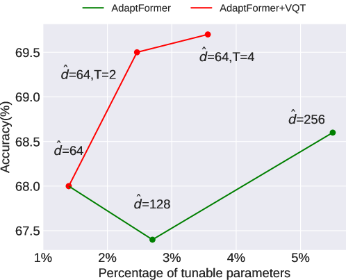
Figure 2: The power of leveraging intermediate features provided by VQT allows AdaptFormer to incorporate additional information from the updated model (red curve), which would not be possible by simply increasing the complexity of the inserted modules (green curve). $\hat{d}$ denotes the bottleneck dimension of AdaptFormer and T represents the number of VQT’s query tokens.

We summarize the results in Table 2, where each row shows the results for one pre-trained backbone, and each column shows the results for one data category. Generally speaking, AdaptFormer and VPT benefit from VQT in most of the scenarios across different data categories and pre-trained backbones. The improvement is more salient in the MAE backbone. Since the MAE pre-training uses the reconstruction objective instead of the classification or contrastive one, we hypothesize that some useful intermediate features for classification may not be propagated to the final layer. With the help of VQT, AdaptFormer and VPT can leverage intermediate features in a more concise and effective way. Additionally, VQT also benefits from AdaptFormer and VPT. In subsection 4.2, we found that directly applying VQT to the pre-trained backbone may not be effective for the Structured category due to the low domain affinity. With the intermediate features updated by AdaptFormer and VPT, VQT can summarize these more relevant features to improve the results for the Structured group. To sum up, the experiment results illustrate that VQT and PETL methods are complementary and mutually beneficial, with the potential to further unleash the power of transfer. We provide detailed results of various pre-trained backbones in Appendix C.6 and the compatibility comparison between Head2Toe and VQT in Appendix C.7.

Methods	Natural	Specialized	Structured
Linear-probing	18.87	53.72	23.70
Fine-tuning	59.29	79.68	53.82
VPT	63.50	79.15	48.58
VQT (Our)	66.00	82.87	52.64

Table 3: Average accuracy on VTAB-1k using the MAE backbone.

To confirm that the improvement mentioned above does not simply come from the increase of tunable parameters, we enlarge AdaptFormer’s added modules by increasing the bottleneck dimension $\hat{d}$ from 64 to 128 and 256 to match the tunable parameter number of AdaptFormer when it is equipped with VQT. As shown in Figure 2, AdaptFormer with VQT significantly outperforms AdaptFormer with larger added modules when the numbers of tunable parameters are similar. This further demonstrates the complementary strength of VQT and AdaptFormer: the improvement by leveraging intermediate features summarized by VQT cannot be achieved by simply increasing the complexity of the inserted modules in AdaptFormer.

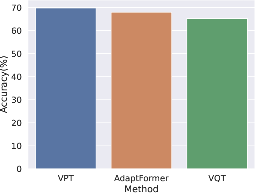
(a)

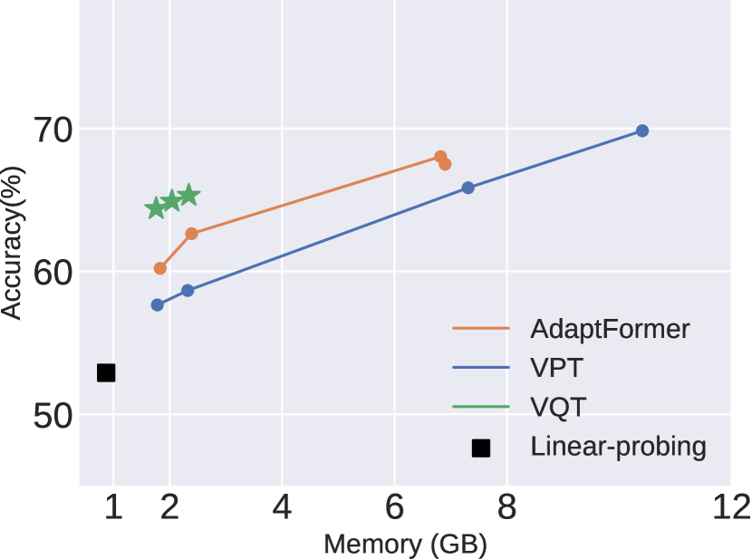
(b)

Figure 3: Comparison under memory constraints. (a) Without constraints, VPT and AdaptFormer slightly outperform VQT. (b) With constraints, VQT performs the best in low-memory regimes.

4.4 Memory Efficient Training

While many PETL methods reduce the number of tunable parameters, they cannot cut down the memory footprint during training by much, and therefore, the evaluation of PETL methods often ignores memory consumption. In real-world scenarios, however, a model is often required to adapt to new data on edge devices for privacy concerns, necessitating the need for methods that can be trained with limited memory. This motivates us to further analyze the accuracy-memory trade-off for VPT, AdaptFormer, and VQT.

As discussed in subsection 3.3, VPT and AdaptFormer require storing the intermediate back-propagation results to update their added parameters, while VQT bypasses the expensive back-propagation because it keeps all the intermediate features intact. To evaluate their performance in the low-memory regime, we only add their inserted parameters to the last few layers to match the memory usage. 3(a) shows the performance of VQT, VPT, and AdaptFormer under their best hyperparameters without memory constraints; 3(b) depicts the accuracy-memory trade-off for these methods. When memory is not a constraint, VPT and AdaptFormer slightly outperform VQT, but they consume 3.8x and 5.9x more memory (GB) than VQT, respectively, as we can see in 3(b).

When memory is a constraint (left side of 3(b)), we see drastic accuracy drops of AdaptFormer and VPT. Although they still surpass linear-probing, VQT outperforms them significantly, suggesting that VQT is a more memory-efficient method thanks to its query-only mechanism.

4.5 Discussion

Layer importance for each category. As VQT leverages the summarized intermediate features for predictions, we investigate which layers produce more critical features for each category. In Figure 4, we show each layer’s importance score computed by averaging the feature importance in the layer. Features in deeper layers are more important for the Natural category, while features from all layers are almost equally important for the Specialized category. Contrastingly, VQT heavily relies on the CLS token for the Structured category. We hypothesize that the low domain affinity between ImageNet and the Structured category may cause the intermediate features to be less relevant, and the model needs to depend more on the CLS token.

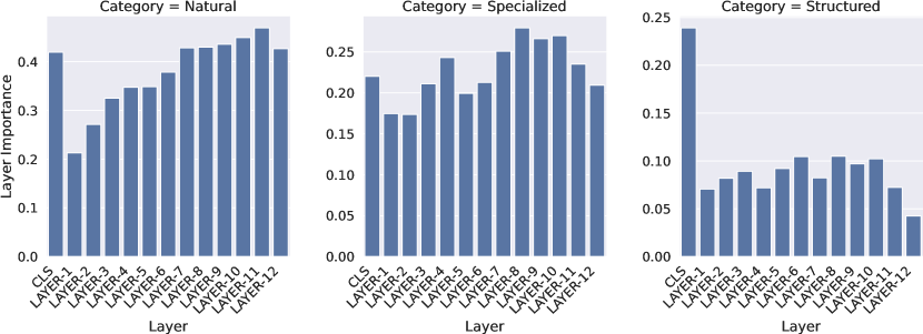
Figure 4: Layer importance for each category in VTAB-1k.

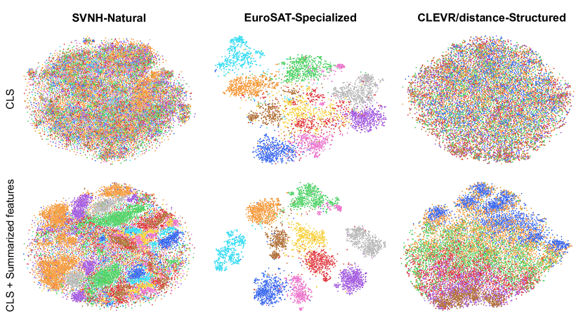
Figure 5: t-SNE visualization of the CLS tokens alone (top) and CLS tokens plus our summarized features (bottom) on 3 tasks from each VTAB’s category. Adding the summarized intermediate features makes the whole features more separable.

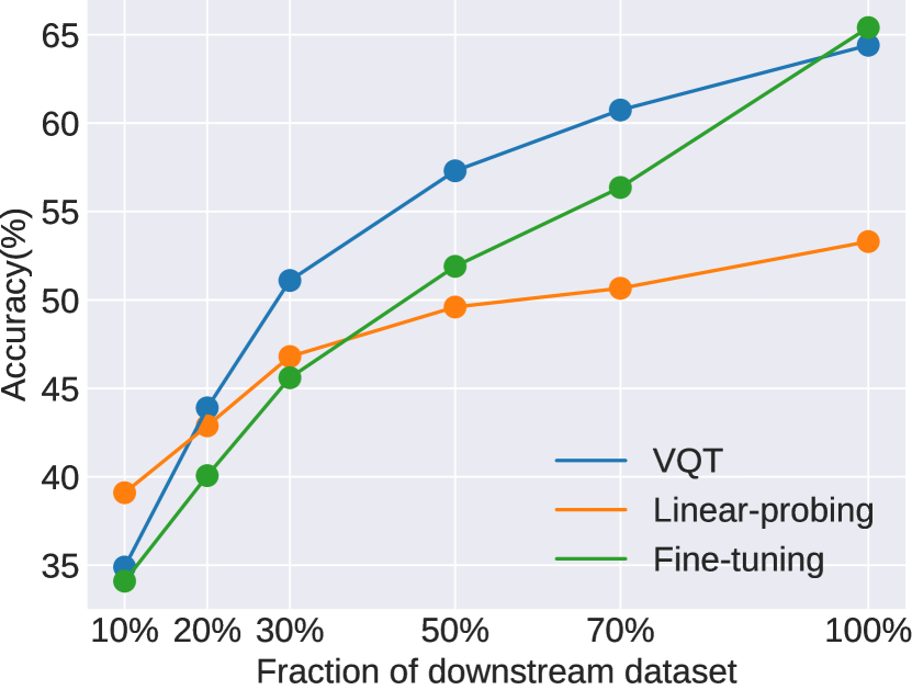
(a)

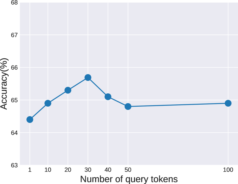
(b)

Figure 6: (a) Average accuracy over the 19 tasks in VTAB-1k using different training data sizes. For each task, 100% means that we use all the 1000 training images. In the 10% data case, we averagely have only 2 images per class. (b) Average accuracy on VTAB-1k using different numbers of query tokens for VQT.

Different downstream data sizes. We further study the effectiveness of VQT under various training data sizes. We reduce the VTAB’s training sizes to {10%, 20%, 30%, 50%, 70%} and compare VQT with Fine-tuning and Linear probing in 6(a). Although fine-tuning slightly outperforms VQT on 100% data, VQT consistently performs better as we keep reducing the training data. On the 10% data case, where we only have 2 images per class on average, Linear probing obtains the best accuracy, but its improvement diminishes and performs much worse than VQT when more data become available. These results show that VQT is more favorable in a wide range of training data sizes.

Number of query tokens. As we use only one query token for VQT in previous experiments, we now study VQT’s performance using more query tokens on VTAB-1k. 6(b) shows that more query tokens can improve VQT, but the accuracy drops when we add more than 40 tokens. We hypothesize that overly increasing the model complexity causes overfitting due to the limited data in VTAB-1k.

Visualization. Figure 5 shows t-SNE [45] visualization of the CLS token and our summarized features for three tasks (SVHN, EuroSAT, and Clevr-Dist), one from each category. Compared with the CLS token alone, adding summarized features makes the whole features more separable, showing the strength of using intermediate features and the effectiveness of our query tokens in summarizing them. We provide the visualization of other tasks in Appendix C.5.

5 Conclusion

We introduced Visual Query Tuning, a simple yet effective approach to aggregate intermediate features of Vision Transformers. By introducing a set of learnable “query” tokens to each layer, VQT leverages the intrinsic mechanism of Transformers to “summarize” rich intermediate features while keeping the intermediate features intact, which allows it to enjoy a memory-efficient training without back-propagation through the entire backbone. Empirically, VQT surpasses Head2Toe, the SOTA method that utilizes intermediate features, and we demonstrate robust and mutually beneficial compatibility between VQT and other PETL methods. Furthermore, VQT is a more memory-efficient approach and achieves much higher performance in a low-memory regime. While VQT only focuses on summarizing features within each layer, we hope our work can pave the way for exploring more effective ways of using features across layers and leveraging intermediate features in transfer learning for other tasks, such as object detection, semantic segmentation and video classification.

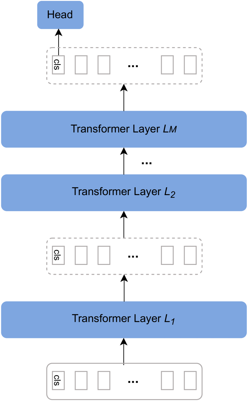
(a)

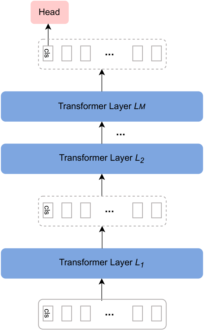
(b)

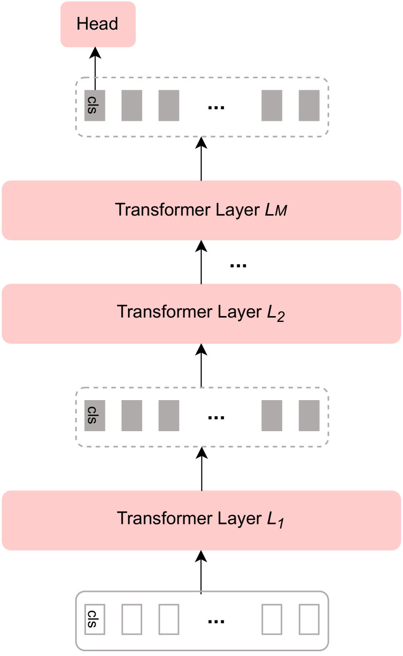
(c)

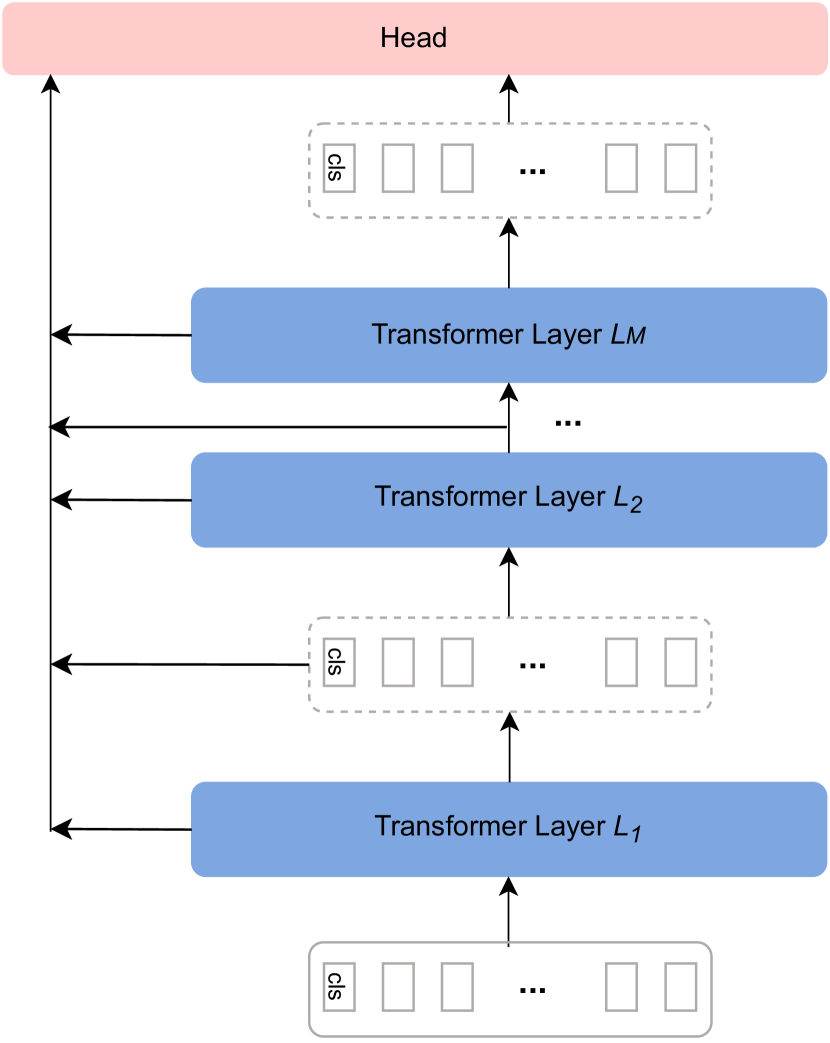
(d)

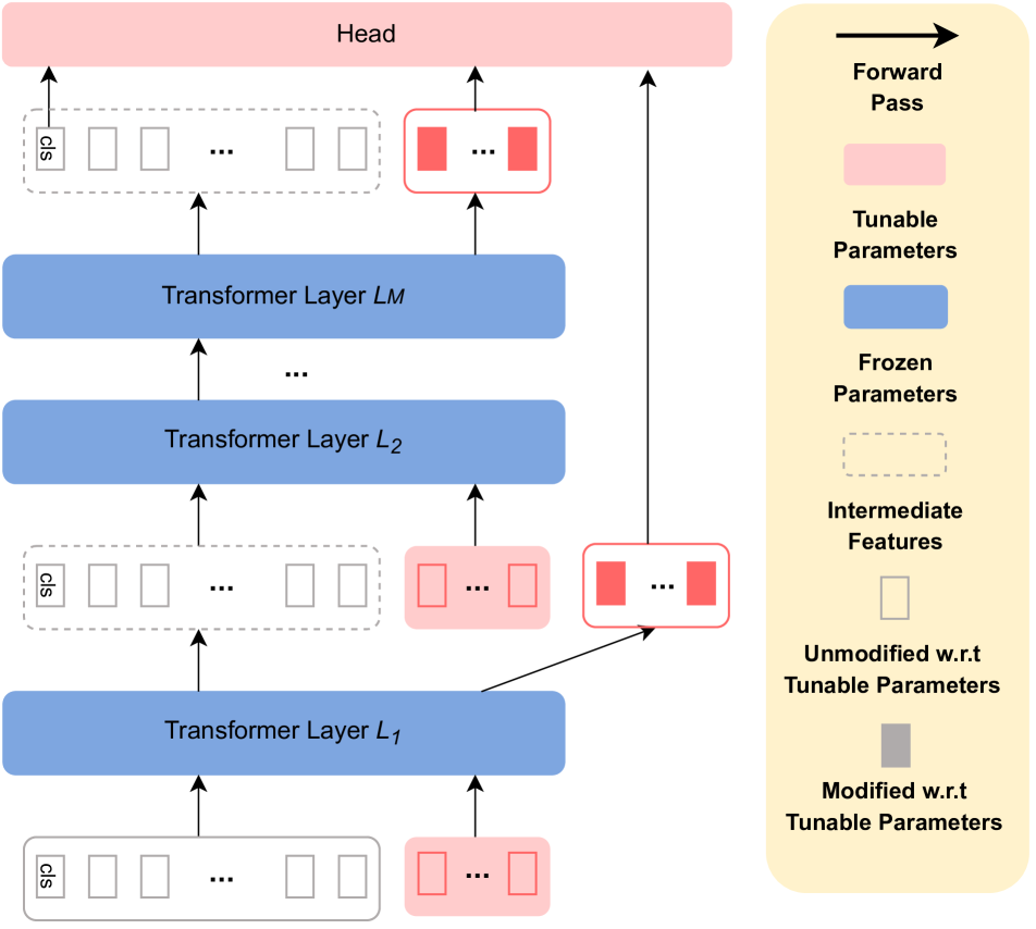
(e)

Figure 7: Conceptual comparison between different transfer learning methods (a) ViT Backbone. (b) Linear-Probing. (c) Fine-Tuning. (d) Head2Toe [15]. (d) VQT (Ours).

Appendix

We provide details omitted in the main paper.

• Appendix A: a conceptual comparison of VQT with other transfer learning methods.

• Appendix B: additional experiment details (cf. section 4 of the main paper).

• Appendix C: additional experiment results and analyses (cf. section 4 of the main paper).

• Appendix D: additional discussions.

Appendix A Conceptual Comparison between VQT and Transfer Learning Methods

We demonstrate the conceptual difference between various transfer learning methods in Figure 7. 7(a) shows the pre-trained ViT backbone. Linear-probing (7(b)) only updates the prediction head and keeps the rest of the backbone unchanged, while fine-tuning (7(c)) updates the whole backbone. Head2Toe (7(d)) takes intermediate outputs of blocks within each Transformer layer for predictions. In contrast, our VQT (7(e)) leverages the summarized intermediate features of each Transformer layer for final predictions.

Appendix B Additional Experiment Details

B.1 Pre-training Setups

In subsection 4.2 and subsection 4.3 of the main paper, we conduct our experiments on three types of pre-trained backbones, Supervised [13], MAE [20], and CLIP [39]. We briefly review these pre-training methods in the following.

Supervised.

Given a pre-training data set $\mathcal{D}_{\text{pre-train}}=\{(\bm{I}_{i},y_{i})\}_{i=0}^{N}$, where $\bm{I}_{i}$ is an image and $y_{i}\in[C]$ is the annotated class label, we aim to train a network that classifies images into $C$ classes. The network consists of a backbone network $f$ to extract features and a linear classifier $h$ to predict class labels. Specifically, let $\bm{p}_{i}=h(f(\bm{I}_{i}))\in\mathbb{R}^{C}$ be the output of the whole network. Each element of $\bm{p}_{i}$ represents the score of $\bm{I}_{i}$ being classified to each of the $C$ classes. We apply the standard cross-entropy loss to maximize the score of classifying $\bm{I}_{i}$ to be the class $y_{i}$. After pre-training, we discard the classifier $h$ and only keep the pre-trained backbone $f$ for learning downstream tasks.

In our experiments, we use ViT-B/16 as the backbone architecture. In subsection 4.2, we use the ImageNet-1K pre-trained backbone following Head2Toe [15]. In subsection 4.3, we use the ImageNet-21K pre-trained backbone following VPT [23]. To save the pre-training time, we use the checkpoints of these backbones released on the official GitHub page of Vision Transformer [13].

MAE.

The learning objective of MAE is to reconstruct an image from its partial observation. Specifically, we divide an input image $\bm{I}$ into $N$ fixed-sized non-overlapping patches $\{\bm{I}^{(n)}\}_{n=1}^{N}$ following ViT [13]. Then, we randomly mask $K\%$ of the patches. Let $\mathcal{U}$ be the set of indices of the unmasked patches and $|\mathcal{U}|=(1-K\%)\times N$. The goal is to reconstruct the masked patches using the unmasked ones $\{\bm{I}^{(i)}|i\in\mathcal{U}\}$. To achieve this, we first process the unmasked patches by a ViT encoder $f$ to generate the output $\bm{Z}_{M}=[{\bm{x}}_{M}^{(i_{1})},\cdots,{\bm{x}}_{M}^{(i_{|\mathcal{U}|})}]$, where $i_{1},\cdots,i_{|\mathcal{U}|}\in\mathcal{U}$. Then, we expand $\bm{Z}_{M}$ to have $N$ tokens by filling $K\%\times N$ mask tokens ${\bm{x}}^{\text{(Mask)}}$ into the positions of the masked patches to generate $\tilde{\bm{Z}}_{M}$. The mask token ${\bm{x}}^{\text{(Mask)}}$ is a learnable parameter and indicates the missing patches to be predicted. Finally, we use a decoder $h$ to generate the reconstructed image $\tilde{\bm{I}}=h(\tilde{\bm{Z}}_{M})$. The whole encoder-decoder network is trained by comparing $\tilde{\bm{I}}$ with $\bm{I}$ by using the mean squared error (MSE). Similar to BERT [25], the loss is computed only on the masked patches. After pre-training, we discard the decoder $h$ and only keep the encoder $f$ as the backbone. In subsection 4.3, we use the ViT-B/16 backbone released in the official MAE [20] GitHub page.

CLIP.

CLIP leverages text captions of images as supervisions for pre-training a visual model. The learning objective is to predict which text caption is paired with which image within a batch. Specifically, given a batch of image-caption pairs $\{(\bm{I}_{i},\bm{C}_{i})\}_{i=1}^{B}$, where $\bm{I}_{i}$ is an image and $\bm{C}_{i}$ is the caption, CLIP uses a image encoder $f$ and a text encoder $h$ to map $\bm{I}_{i}$ and $\bm{C}_{i}$ into a multi-modal embedding space, respectively. Let $\bm{Z}_{I}=[f(\bm{I}_{1}),\cdots,f(\bm{I}_{B})]\in\mathbb{R}^{D\times B}$ and $\bm{Z}_{C}=[h(\bm{C}_{1}),\cdots,h(\bm{C}_{B})]\in\mathbb{R}^{D\times B}$ be the output image and text features. We then compute pair-wise similarity between the columns of $\bm{Z}_{I}$ and $\bm{Z}_{C}$, resulting in $\bm{S}=\bm{Z}_{I}^{T}\bm{Z}_{C}\in\mathbb{R}^{B\times B}$. The diagonal elements in $\bm{S}$ are the scores for the correct image-caption pairings while the rest elements are incorrect pairings. CLIP minimizes the cross-entropy losses computed on the rows and the columns of $\bm{S}$ to learn $f$ and $h$. After pre-training, we discard $h$ and keep the vision encoder $f$ as the pre-trained backbone. In subsection 4.3, we use the ViT-B/16 backbone released in the official CLIP [39] GitHub page.

B.2 Feature Selection via Group Lasso

We provide more details for feature selection based on group lasso as mentioned in subsection 3.2 of the main paper. In VQT, we concatenate the newly summarized features $\{\bm{Z}_{m+1}^{\prime}\}_{m=0}^{M-1}$ with the final “CLS” token ${\bm{x}}_{M}^{\text{(Class)}}$ for linear probing. Let $\bm{H}_{\text{all}}\in\mathbb{R}^{MDT+D}$ be the concatenated features and $\bm{W}_{\text{all}}\in\mathbb{R}^{(MDT+D)\times C}$ be the weights of the linear classifier, where $C$ is the number of classes. After we learn the additional query tokens in VQT, we can freeze them and optionally employ group lasso to reduce the dimensionality of $\bm{H}_{\text{all}}$. Specifically, we follow Head2Toe [15] to first train the linear classification head with the group-lasso regularization $|\bm{W}_{\text{all}}|_{2,1}$, which encourages the $\ell_{2}$ norm of the rows of $\bm{W}_{\text{all}}$ to be sparse. Then, the importance score of the $i$-th feature in $\bm{H}_{\text{all}}$ is computed as the $\ell_{2}$ norm of the $i$-th row of $\bm{W}_{\text{all}}$. Finally, we select a fraction $F$ of the features $\bm{H}_{\text{all}}$ with the largest importance scores and train a new linear head with the selected features.

B.3 Parameter Efficiency in Section 4.2

We provide the number of parameters for the transfer learning methods compared in subsection 4.2 of the main paper.

Linear-probing and full fine-tuning.

For each task, linear probing only trains the prediction head and keeps the whole pre-trained backbone unchanged. Therefore, we only need to maintain one copy of the backbone that can be shared across all the downstream tasks. Contrastingly, full fine-tuning updates the whole network, including the backbone and the head, for each task. After training, each task needs to individually store its own fine-tuned backbone, thereby requiring more parameters.

VQT vs. Head2Toe.

In subsection 4.2 of the main paper, We compare VQT with Head2Toe by matching the number of tunable parameters for each task in VTAB-1k. We provide details for this setup. More comparisons of VQT and Head2Toe can be found in subsection C.1.

Head2Toe [15] takes intermediate features from multiple distinct steps inside the pre-trained ViT backbone. For the features from each step, Head2Toe chooses a window size and a stride to perform average pooling to reduce the dimensionality. After concatenating the pooled intermediate features, Head2Toe further decides the fraction $F$ for feature selection. In Head2Toe, the pooling window size, pooling stride and $F$ are hyper-parameters picked based on validation accuracy.

For fair comparisons of VQT and Head2Toe [15], we match their numbers of tunable parameters used in different tasks. As both VQT and Head2Toe leverage intermediate features while keeping the backbone unchanged, the tunable parameters mainly reside in the final linear head. We focus on matching the feature dimension input to the classifier. First, we divide the 19 tasks in VTAB-1k into three groups; each group corresponds to a pair of pooling window sizes and strides that Head2Toe uses to generate the features before feature selection. Specifically, in the three groups, Head2Toe generates 68K-, 815K-, and 1.8M-dimensional features, respectively. Next, for simplicity, we set $F=0.1$, which is the maximal $F$ in Head2Toe’s hyper-parameter search grid, for Head2Toe in all the 19 tasks. These results are obtained using the official Head2Toe released code. For VQT, we choose $T$ and $F$ to match the final feature dimensions (after feature selection) used in Head2Toe. Specifically, we use $T=1$ and $F=0.7$, $T=10$ and $F=1.0$, and $T=20$ and $F=1.0$ for the three task groups, respectively.

Comparison on the number of parameters.

We summarize the number of parameters needed for all the 19 VTAB-1k tasks in Table 4. As linear-probing shares the backbone among tasks and only adds linear heads that take the final “CLS” token, it only requires $1.01\times$ of the ViT-B/16 backbone parameters. By contrast, fine-tuning consumes $19.01\times$ of the ViT-B/16 because each task maintains its own fine-tuned backbone. Compared to linear probing, VQT and Head2Toe use larger feature dimensions for prediction, thereby increasing the number of parameters in the final linear heads. Even so, VQT and Head2Toe are still parameter-efficient and need only $1.22\times$ and $1.20\times$ of the backbone parameters to learn 19 tasks.

Methods	Total # of parameters
Scratch	$19.01\times$
Linear-probing	$1.01\times$
Fine-tuning	$19.01\times$
Head2Toe	$1.20\times$
VQT (Our)	$1.22\times$

Table 4: Total numbers of parameters needed for all the 19 tasks, for the methods compared in Table 1. Each number represents how many times of one ViT-B/16 backbone’s parameters (86M) are needed.

B.4 Additional Training Details

We provide training details for VQT, VPT [23] and AdaptFormer [10] used in section 4.

For each task in VTAB-1k, we perform an 80/20 split on the 1K training images to form a training/validation set for hyper-parameter searching. After we pick the best hyper-parameters that yield the best validation accuracy, we use them for training on the original 1K training images. Finally, we report the accuracy on the testing set.

For training VQT with the ImageNet-1K backbone, we set $T$ to match the number of tunable parameters with Head2Toe as described in subsection B.2. For training VQT with the MAE backbone (results reported in Table 3), we simply set $T=1$ for all tasks in VTAB-1k. We then perform a hyper-parameter search to select the best learning rate from $\{1.0,0.5,0.25,0.1,0.05\}$ and the best weight decay from $\{0.01,0.001,0.0001,0.0\}$. We use the Adam optimizer to train VQT for 100 epochs, and the learning rate follows the cosine schedule.

For training VPT with the ImageNet-21K and the MAE backbones, we use each task’s best number of prompt tokens, which are released in VPT’s GitHub page. Since the VPT paper does not use the CLIP backbone, we simply set the number of tokens to $1$ for all tasks in this case. We conduct a hyper-parameter search to pick the best learning rate from $\{1.0,0.5,0.25,0.1,0.05\}$ and the best weight decay from $\{0.01,0.001,0.0001,0.0\}$. We train VPT using the Adam optimizer for 100 epochs with the cosine learning rate schedule.

Finally, when training AdaptFormer on all backbones, we use the bottleneck dimension $\hat{d}=64$ and the scaling factor $s=0.1$ following [10]. We similarly search the best learning rate from $\{1.0,0.5,0.25,0.1,0.05\}$ and the best weight decay from $\{0.01,0.001,0.0001,0.0\}$ using the validation set. The AdaptFormer is trained with the Adam optimizer for 100 epochs, and the learning rate decay follows the cosine schedule.

Appendix C Additional Experiments and Analyses

C.1 More Comparison with Head2Toe

	Natural								Specialized					Structured
Method	CIFAR-100	Caltech101	DTD	Flowers102	Pets	SVHN	Sun397	Mean	Camelyon	EuroSAT	Resisc45	Retinopathy	Mean	Clevr-Count	Clevr-Dist	DMLab	KITTI-Dist	dSpr-Loc	dSpr-Ori	sNORB-Azim	sNORB-Elev	Mean	Overall Mean
Head2Toe	58.2	87.3	64.5	85.9	85.4	82.9	35.1	71.3	81.2	95.0	79.9	74.1	82.6	49.3	58.4	41.6	64.4	53.3	32.9	33.5	39.4	46.6	63.3
VQT (Ours)	58.5	89.5	66.7	89.9	88.8	79.7	35.1	72.6	82.4	96.2	84.4	74.8	84.5	50.5	57.1	42.7	77.9	69.2	43.6	24.1	32.0	49.6	65.4

Table 5: Head2Toe and VQT’s test accuracies on the VTAB-1k benchmark with ViT-B/16 pre-trained on ImageNet-1K. In this comparison, we do not set parameter constraints and use the validation set to choose the best feature dimension based on accuracy. ”Mean” denotes the average accuracy for each category and ”Overall Mean” shows the average accuracy over 19 tasks.

In Table 1 of the main paper, we have compared VQT with Head2Toe under the constraint of using a similar number of tunable parameters, as mentioned in subsection B.3. To further evaluate the limit of VQT, we drop this constraint and allow both VQT and Head2Toe to select the best feature dimensions based on accuracy. Specifically, we pick the best feature fraction $F$ for VQT using the validation set and compare it with the best Head2Toe results, which are also obtained by selecting the best feature dimension via hyper-parameter tuning, reported in their paper [15]. Table 5 shows the results of Head2Toe and VQT without the parameter constraint. VQT still significantly outperforms Head2Toe on 15 out of 19 tasks across the Natural, Specialized and Structured categories of VTAB-1k, demonstrating the effectiveness of the summarized intermediate features in VQT. We also compare Head2Toe and VQT on different pre-trained setups. As shown in Table 6, VQT consistently outperforms Head2Toe on supervised, self-supervised (MAE) and image-language (CLIP) pre-trained backbones. We used the best hyper-parameters from the Head2Toe paper for the ImageNet-1K backbone, and we only performed the learning rate and weight decay hyper-parameters search for the MAE and CLIP model. We match the number of tunable parameters in VQT and Head2Toe for fair comparisons.

Methods	Natural	Specialized	Structured	Mean
ImageNet-1K
H2T	68.9	82.9	46.3	62.3
VQT	72.7	84.5	49.3	65.3
MAE
H2T	55.6	80.3	44.4	55.7
VQT	66.0	82.9	53.5	63.9
CLIP
H2T	69.3	82.0	33.8	57.0
VQT	77.7	83.7	51.3	67.9

Table 6: Performance comparison between HEAD2TOE (H2T) and VQT on various backbones.

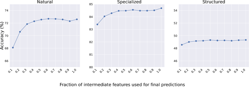
Figure 8: Average accuracy on VTAB-1k using different fractions of intermediate features for VQT.

C.2 Robustness to Different Feature Fractions

We study the robustness of VQT using different fractions of the intermediate features for prediction. Given a fraction $F$, we follow the strategy mentioned in subsection B.2 to select the best features. As shown in Figure 8, VQT is able to maintain its accuracy, with less than $1\%$ drop, even when we discard $60\%$ of the features. On the Structured category in VTAB-1k, we can even drop up to $90\%$ of the features for VQT without largely degrading its performance. These results reveal the potential of further compressing VQT to reduce more parameters.

C.3 Different Vision Transformer Backbones

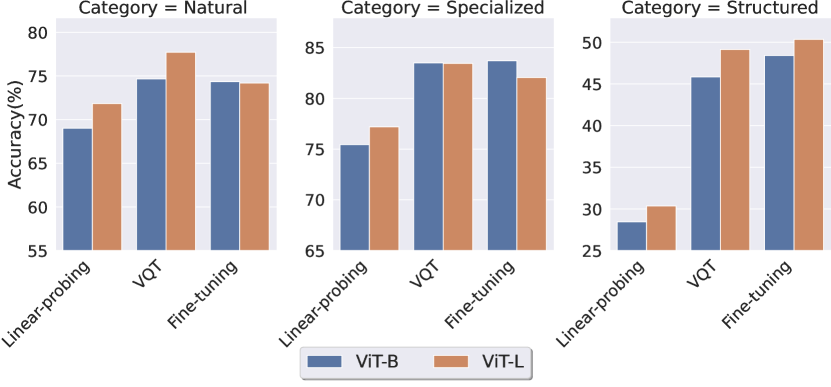
Figure 9: Performance comparison between linear-probing, fine-tuning and VQT on ViT-Base (86M parameters) and ViT-Large (307M parameters) pretrained on ImageNet-21K

Figure 9 shows the performance comparison between linear-probing, fine-tuning and VQT on ViT-Base (86M parameters) and ViT-Large (307M parameters) pretrained on ImageNet-21K. Generally speaking, all methods perform better on ViT-L than ViT-B due to higher model complexity. In the Natural and Specialized category, VQT has similar performance as fine-tuning on ViT-B and outperforms fine-tuning on ViT-L. As explained in subsection 4.2, the Natural and Specialized categories have stronger domain affinities with the source domain (ImageNet). Thus, both pre-trained backbones can generate more relevant intermediate features for similar domains. In the Structured category, fine-tuning slightly surpasses VQT on both backbones due to the difference between the pretrained dataset and the Structured category.

C.4 Variants of VQT

We ablate different design choices on the ViT-B pretrained on ImageNet-21K and evaluate them on the VTAB dataset.

Summarized feature aggregation within layers.

VQT relies on each layer’s summarized features (the outputs of query tokens) for predictions. Although adding a suitable number of tokens can improve the performance as shown in 6(b), we investigate if we can effectively aggregate the summarized features within a Transformer layer to reduce the dimensionality by two approaches: (1) average pooling and (2) weighted-sum, as shown in 12(a). Specifically, (1) we perform pooling to average T output tokens back to 1 token; (2) we learn a set of weights for each layer to perform weighted-sum over T output tokens. After the aggregation step, the size of the summarized features for each layer will be changed from $\mathbb{R}^{D\times T}$ to $\mathbb{R}^{D\times 1}$.

11(a) and 11(b) show the aggregation performance for T=10 and T=20 respectively. When we use T=10, average pooling performs similarly to T=10 and outperforms T=1 and weighted-sum. However, the trend is reversed when we use T=20; weighted-sum surpasses average pooling and T=1. To strike a balance between performance and efficiency, we suggest utilizing the validation set to choose a good within-layer aggregation method for a downstream dataset.

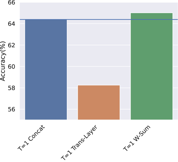
Figure 10: Performance comparison for different across-layer aggregation methods when T=1. The blue line shows the accuracy for T=1 Concat. W-Sum is a more efficient and effective way to aggregate summarized features across layers since it reduces the dimensionality and performs better.

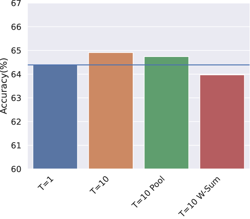
(a)

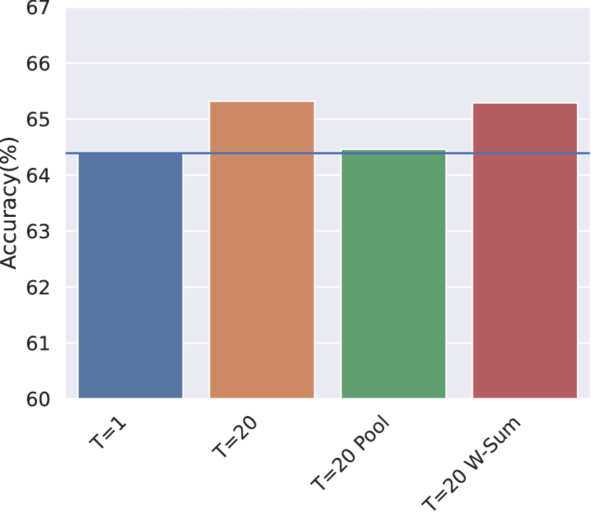
(b)

Figure 11: Performance comparison for different within-layer aggregation methods when T=10 and T=20, where ”pool” and ”W-Sum” refers to average pooling and weighted sum, respectively. The blue line shows the accuracy for T=1. Note that the summarized feature dimension for T=10 (20) pool (w-Sum) is the same as the one for T=1.

Summarized feature aggregation across layers.

This section explores how to aggregate the summarized features (the outputs of query tokens) across layers. Instead of concatenation (Concat), the default method we use in the main paper, we try feeding the summarized features from all layers to a randomly initialized Transformer layer with the CLS token from the last Transformer layer and use the output of the CLS token for prediction, dubbed Trans-Layer. We also try to perform weighted-sum over all the summarized features, dubbed W-Sum. When T=1, the dimension for Concat is $\mathbb{R}^{D\times M}$ where $M$ is the number of Transformer layers in the backbone and the dimension for Trans-Layer and W-Sum is $\mathbb{R}^{D\times 1}$. The across-layer aggregation methods are demonstrated in 12(b).

As shown in Figure 10, Trans-Layer is way behind Concat. We hypothesize that the limited number of images per task may not be sufficient to train a randomly initialized Transformer layer. On the contrary, W-Sum outperforms the default Concat, which is surprising for us since the same dimension of the summarized feature in different layers may represent different information, and thus, the summarized feature from different layers may not be addable. However, based on this result, we hypothesize that the skip connection in each layer can be the cause of the addibility of summarized features from different layers. We believe studying more effective and efficient aggregation methods for the summarized features is an interesting future direction.

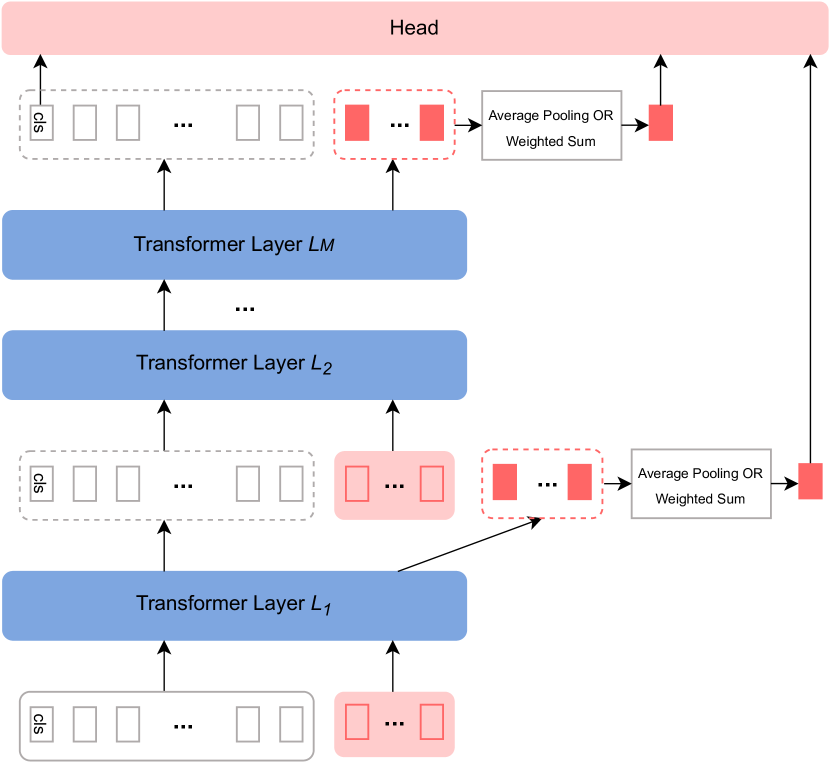
(a)

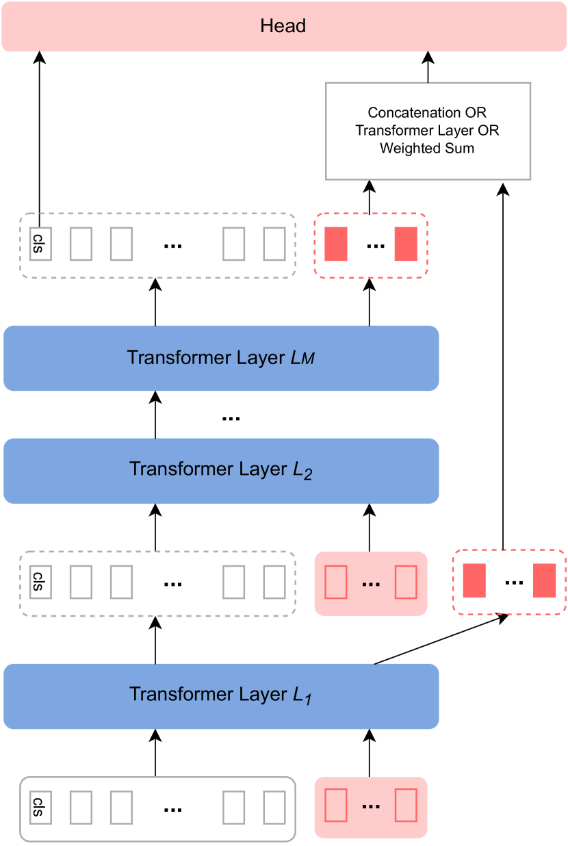
(b)

Figure 12: (a) shows the within-layer aggregate methods. Multiple output query tokens within the same layer can be aggregated through average pooling or weighted sum. (b) shows the across-layer aggregation methods. Output query tokens from different layers can be aggregated through concatenation, weighted sum or another randomly initialized Transformer layer.

C.5 t-SNE Visualization for More Datasets

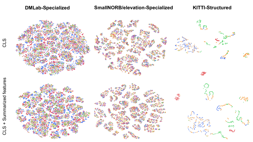
(a)

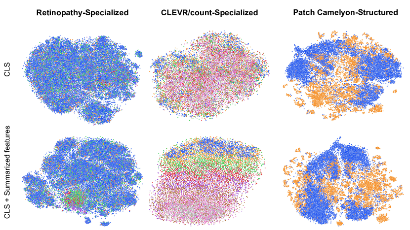
(b)

Figure 13: t-SNE visualization of the CLS tokens alone (top) and CLS tokens plus our summarized features (bottom) on more tasks from VTAB. Adding the summarized intermediate features makes the whole features more separable. We include tasks that have less or equal to 10 classes for visualization.

We present t-SNE visualizations of the CLS token and our summarized features for more tasks in Figure 13. Similar to Figure 5, adding summarized features makes the whole features more separable than the CLS token alone, demonstrating the benefit of using intermediate features and the advantage of our query tokens in summarizing them.

C.6 Results for All Tasks on Different Backbones

Table 8 shows the per-task accuracies for 19 tasks in VTAB on different ViT-B backbones, including CLIP, MAE and Supervised ImageNet-21K.

C.7 Compatibility comparison between VQT and H2T

We compare the compatibility performance between HEAD2TOE and VQT with VPT and AdaptFormer (AF). For a fair comparison, we ensure that the output feature dimension is the same as the original one (D=768 in ViT) when we combine VPT and AdaptFormer with HEAD2TOE and VQT. We use the default feature selection method in the original paper for HEAD2TOE and the weighted-sum approach (see subsection C.4 for details) for VQT. Table 7 shows the results on ImageNet-1k pre-trained backbone and VQT demonstrates more competitive compatibility performance than HEAD2TOE.

Methods	Natural	Specialized	Structured	Mean
VPT	74.9	82.9	53.9	65.9
VPT+H2T	69.1	81.1	50.9	64.0
VPT+VQT	76.8 (6/7)	83.8(2/4)	53.4(6/8)	68.4
AF	73.4	80.1	47.3	63.8
AF+H2T	69.4	82.3	51.4	64.5
AF+VQT	77.0(7/7)	84.6(2/4)	53.4(6/8)	68.7

Table 7: Compatibility comparison between HEAD2TOE (H2T) and VQT on VPT and AdaptFormer (AF). The (/) represents the number of wins compared to baselines and baselines+H2T. The results are based on ImageNet-1k pre-trained backbone.

	Natural								Specialized					Structured
Method	CIFAR-100	Caltech101	DTD	Flowers102	Pets	SVHN	Sun397	Mean	Camelyon	EuroSAT	Resisc45	Retinopathy	Mean	Clevr-Count	Clevr-Dist	DMLab	KITTI-Dist	dSpr-Loc	dSpr-Ori	sNORB-Azim	sNORB-Elev	Mean	Overall Mean
CLIP backbone
AdaptFormer	73.7	93.2	75.2	96.8	90.7	92.7	56.1	82.6	83.3	95.7	87.8	73.6	85.1	76.5	61.9	49.6	84.1	84.6	55.4	29.5	45.7	60.9	74.0
AdaptFormer+VQT	71.3	95.3	77.1	96.2	90.6	93.3	51.2	82.1	84.8	96.4	88.7	73.4	85.8	75.8	62.6	52.4	83.8	91.8	54.6	33.6	46.5	62.6	74.7
VPT	66.3	90.1	73.7	94.7	90.3	91.6	56.0	80.4	83.3	93.4	87.3	75.6	84.9	41.5	57.5	52.3	80.7	65.1	54.3	27.7	28.4	50.9	68.9
VPT+VQT	70.8	95.1	72.7	93.8	89.8	93.5	54.8	81.5	85.2	95.7	89.7	74.8	86.3	52.5	62.6	55.3	84.1	77.1	56.4	34.6	35.1	57.2	72.3
MAE backbone
AdaptFormer	53.5	90.1	60.3	83.3	81.4	83.0	29.6	68.7	83.0	93.9	74.4	73.8	81.3	77.8	60.3	44.0	79.5	75.9	53.1	30.3	45.6	58.3	67.0
AdaptFormer+VQT	56.8	90.4	63.7	86.8	80.7	89.7	29.7	71.1	84.5	95.4	80.9	72.5	83.3	65.9	58.5	46.5	84.0	82.2	53.2	32.1	51.1	59.2	68.6
VPT	45.5	88.9	62.2	75.1	73.2	75.2	24.4	63.5	80.1	94.6	68.3	73.6	79.1	69.5	58.2	39.4	70.8	53.6	51.2	20.4	25.5	48.6	60.5
VPT+VQT	48.9	90.3	65.2	87.4	81.8	75.9	26.0	67.9	81.4	95.1	80.8	73.6	82.7	63.3	59.2	44.4	80.2	46.5	52.7	22.8	28.4	49.7	63.4
Supervised ImageNet-21K backbone
AdaptFormer	79.9	89.8	68.5	98.0	88.3	81.4	54.8	80.1	80.3	95.4	81.1	72.3	82.3	71.0	55.0	42.3	68.8	65.9	45.1	24.9	29.8	50.3	68.0
AdaptFormer+VQT	77.1	93.7	68.2	98.2	89.8	84.1	45.9	79.6	82.1	96.2	85.6	73.2	84.3	71.4	54.9	44.5	72.3	76.7	45.2	27.6	31.3	53.0	69.4
VPT	79.8	89.9	67.5	98.0	87.0	79.4	52.3	79.1	83.5	96.0	83.7	75.2	84.6	68.1	60.1	43.0	74.8	74.4	44.4	30.0	40.2	54.4	69.9
VPT+VQT	76.8	92.6	69.2	98.3	87.8	81.6	46.2	78.9	81.3	96.3	84.7	72.4	83.7	59.6	60.3	43.0	77.6	79.3	46.0	31.2	39.5	54.6	69.7

Table 8: Test accuracies for AdaptFormer, VPT and their combinations with VQT on the VTAB-1k benchmark on ViT-B/16 pre-trained with CLIP, MAE and Supervised ImageNet-21K. ”Mean” denotes the average accuracy for each category and ”Overall Mean” shows the average accuracy over 19 tasks.

Appendix D Additional Discussions

D.1 More Discussions on Memory Usage

As mentioned in the last paragraph of subsection 3.3 and as shown in subsection 4.4, since VQT keeps all the intermediate features intact and only learns to tune the query tokens and the prediction head, the training process bypasses the expensive back-propagation steps and does not require storing any intermediate gradient results, making it very memory-efficient. As shown in 1(a), VPT needs to run back-propagation (red arrow lines) through the huge backbone in order to update the inserted prompts. On the contrary, VQT only needs gradients for the query tokens because all intermediate output features are unchanged, as shown in 1(b).

D.2 Cost of VQT and AdaptFormer

In subsection 4.3, to confirm that the improvement mentioned above does not simply come from the increase of tunable parameters, we enlarge AdaptFormer’s added modules by increasing the bottleneck dimension $\hat{d}$ from 64 to 128 and 256 to match the tunable parameter number of AdaptFormer when equipped with VQT. Here, we show the detailed parameter calculation in Figure 2. The additional parameters for AdaptFormer and VQT can be calculated as $\hat{d}\times 2\times D\times M$ and $\underbrace{T\times D\times M}_{\text{query tokens}}+\underbrace{T\times D\times M\times C}_{\text{prediction head}}$, respectively where $\hat{d}$ denotes the bottleneck dimension of AdaptFormer; $D$ is the embedding dimension; $M$ is the number of Transformer layer; T represents the number of VQT’s query tokens; $C$ denotes the average number of classes in VTAB, and we round it to 50 for simplicity. The numbers of tunable parameters and percentages of tunable parameters over ViT-B’s number of parameters (86M) for AdaptFormer and AdaptFormer+VQT are shown in Table 9.

D.3 Training Efficiency

In this subsection, we point out another potential advantage of VQT besides its parameter and memory efficiency — training efficiency (i.e., the number of floating-point operations and the overall wall-clock time in training). This can be seen from two aspects.

On the one hand, since VQT does not change the original intermediate features obtained from the pre-trained backbone but only learns to combine them, we can pre-compute them for all the downstream data and store them in the hard drive or even random access memory (RAM) for later training (epochs). As mentioned in subsection B.4, we perform $100$ epochs for learning the query tokens in VQT, in which we indeed only need to compute the intermediate features once in the first epoch, and reuse them in later epochs. Given a standard ViT-B with 12 Transformer layers and 197 embedding tokens of size 768 for each layer, all the intermediate features for an image amount to “$12\times 197\times 768$” 32-bit floats (7MB); storing them for a task in VTAB with 1K images only requires 7GB in the hard drive or RAM. With all the pre-computed intermediate features, we can parallelize the forward and backward passes of the 12 layers at the same time, potentially making the training process $12\times$ faster.

On the other hand, since VQT only uses the outputs of the newly introduced query tokens for predictions, during the forward pass within each layer, we just need to pass the MSA features corresponding to these tokens to the MLP block, making it additionally faster on top of the cross-layer parallelization mentioned above.

AdaptFormer	$\hat{d}=64$	$\hat{d}=128$	$\hat{d}=256$
Tunable parameters #	1179648	2359296	4718592
Tunable parameters %	1.37%	2.74%	5.49%
AdaptFormer+VQT	$\hat{d}=64$ &	$\hat{d}=64$ & $T=2$	$\hat{d}=64$ & $T=4$
Tunable parameters #	1179648	2119680	3059712
Tunable parameters %	1.37%	2.46%	3.56%

Table 9: Numbers of tunable parameters and percentages of tunable parameters over ViT-B’s number of parameters (86M) for AdaptFormer with different bottleneck dimensions and AdaptFormer+VQT with different numbers of query tokens.

References

- [1] Andreas Argyriou, Theodoros Evgeniou, and Massimiliano Pontil. Multi-task feature learning. Advances in neural information processing systems, 19, 2006.
- [2] Anurag Arnab, Mostafa Dehghani, Georg Heigold, Chen Sun, Mario Lučić, and Cordelia Schmid. Vivit: A video vision transformer. In Proceedings of the IEEE/CVF International Conference on Computer Vision, pages 6836–6846, 2021.
- [3] Akari Asai, Mohammadreza Salehi, Matthew E Peters, and Hannaneh Hajishirzi. Attentional mixtures of soft prompt tuning for parameter-efficient multi-task knowledge sharing. arXiv preprint arXiv:2205.11961, 2022.
- [4] Sean Bell, C Lawrence Zitnick, Kavita Bala, and Ross Girshick. Inside-outside net: Detecting objects in context with skip pooling and recurrent neural networks. In Proceedings of the IEEE conference on computer vision and pattern recognition, pages 2874–2883, 2016.
- [5] Elad Ben Zaken, Yoav Goldberg, and Shauli Ravfogel. BitFit: Simple parameter-efficient fine-tuning for transformer-based masked language-models. In Proceedings of the 60th Annual Meeting of the Association for Computational Linguistics (Volume 2: Short Papers), pages 1–9. Association for Computational Linguistics, 2022.
- [6] Tom Brown, Benjamin Mann, Nick Ryder, Melanie Subbiah, Jared D Kaplan, Prafulla Dhariwal, Arvind Neelakantan, Pranav Shyam, Girish Sastry, Amanda Askell, et al. Language models are few-shot learners. Advances in neural information processing systems, 33:1877–1901, 2020.
- [7] Nicolas Carion, Francisco Massa, Gabriel Synnaeve, Nicolas Usunier, Alexander Kirillov, and Sergey Zagoruyko. End-to-end object detection with transformers. In European conference on computer vision, pages 213–229. Springer, 2020.
- [8] Mathilde Caron, Hugo Touvron, Ishan Misra, Hervé Jégou, Julien Mairal, Piotr Bojanowski, and Armand Joulin. Emerging properties in self-supervised vision transformers. In Proceedings of the IEEE/CVF International Conference on Computer Vision, pages 9650–9660, 2021.
- [9] Hanting Chen, Yunhe Wang, Tianyu Guo, Chang Xu, Yiping Deng, Zhenhua Liu, Siwei Ma, Chunjing Xu, Chao Xu, and Wen Gao. Pre-trained image processing transformer. In Proceedings of the IEEE/CVF Conference on Computer Vision and Pattern Recognition, pages 12299–12310, 2021.
- [10] Shoufa Chen, Chongjian Ge, Zhan Tong, Jiangliu Wang, Yibing Song, Jue Wang, and Ping Luo. Adaptformer: Adapting vision transformers for scalable visual recognition. arXiv preprint arXiv:2205.13535, 2022.
- [11] Xinlei Chen, Saining Xie, and Kaiming He. An empirical study of training self-supervised vision transformers. In Proceedings of the IEEE/CVF International Conference on Computer Vision, pages 9640–9649, 2021.
- [12] Fahim Dalvi, Hassan Sajjad, Nadir Durrani, and Yonatan Belinkov. Analyzing redundancy in pretrained transformer models. In Proceedings of the 2020 Conference on Empirical Methods in Natural Language Processing (EMNLP), pages 4908–4926, 2020.
- [13] Alexey Dosovitskiy, Lucas Beyer, Alexander Kolesnikov, Dirk Weissenborn, Xiaohua Zhai, Thomas Unterthiner, Mostafa Dehghani, Matthias Minderer, Georg Heigold, Sylvain Gelly, Jakob Uszkoreit, and Neil Houlsby. An image is worth 16x16 words: Transformers for image recognition at scale. In International Conference on Learning Representations, 2021.
- [14] Seongha Eom, Taehyeon Kim, and Se-Young Yun. Layover intermediate layer for multi-label classification in efficient transfer learning. In Has it Trained Yet? NeurIPS 2022 Workshop, 2022.
- [15] Utku Evci, Vincent Dumoulin, Hugo Larochelle, and Michael C Mozer. Head2toe: Utilizing intermediate representations for better transfer learning. In International Conference on Machine Learning, pages 6009–6033. PMLR, 2022.
- [16] Meng-Hao Guo, Jun-Xiong Cai, Zheng-Ning Liu, Tai-Jiang Mu, Ralph R Martin, and Shi-Min Hu. Pct: Point cloud transformer. Computational Visual Media, 7(2):187–199, 2021.
- [17] Kai Han, Yunhe Wang, Hanting Chen, Xinghao Chen, Jianyuan Guo, Zhenhua Liu, Yehui Tang, An Xiao, Chunjing Xu, Yixing Xu, et al. A survey on vision transformer. IEEE transactions on pattern analysis and machine intelligence, 2022.
- [18] Bharath Hariharan, Pablo Arbeláez, Ross Girshick, and Jitendra Malik. Hypercolumns for object segmentation and fine-grained localization. In Proceedings of the IEEE conference on computer vision and pattern recognition, pages 447–456, 2015.
- [19] Junxian He, Chunting Zhou, Xuezhe Ma, Taylor Berg-Kirkpatrick, and Graham Neubig. Towards a unified view of parameter-efficient transfer learning. In International Conference on Learning Representations, 2021.
- [20] Kaiming He, Xinlei Chen, Saining Xie, Yanghao Li, Piotr Dollár, and Ross Girshick. Masked autoencoders are scalable vision learners. In Proceedings of the IEEE/CVF Conference on Computer Vision and Pattern Recognition, pages 16000–16009, 2022.
- [21] Kaiming He, Xiangyu Zhang, Shaoqing Ren, and Jian Sun. Deep residual learning for image recognition. In Proceedings of the IEEE conference on computer vision and pattern recognition, pages 770–778, 2016.
- [22] Yun He, Steven Zheng, Yi Tay, Jai Gupta, Yu Du, Vamsi Aribandi, Zhe Zhao, YaGuang Li, Zhao Chen, Donald Metzler, et al. Hyperprompt: Prompt-based task-conditioning of transformers. In International Conference on Machine Learning, pages 8678–8690. PMLR, 2022.
- [23] Menglin Jia, Luming Tang, Bor-Chun Chen, Claire Cardie, Serge Belongie, Bharath Hariharan, and Ser-Nam Lim. Visual prompt tuning. In European Conference on Computer Vision (ECCV), 2022.
- [24] Shibo Jie and Zhi-Hong Deng. Convolutional bypasses are better vision transformer adapters. arXiv preprint arXiv:2207.07039, 2022.
- [25] Jacob Devlin Ming-Wei Chang Kenton and Lee Kristina Toutanova. Bert: Pre-training of deep bidirectional transformers for language understanding. In Proceedings of NAACL-HLT, pages 4171–4186, 2019.
- [26] Salman Khan, Muzammal Naseer, Munawar Hayat, Syed Waqas Zamir, Fahad Shahbaz Khan, and Mubarak Shah. Transformers in vision: A survey. ACM computing surveys (CSUR), 54(10s):1–41, 2022.
- [27] Simon Kornblith, Jonathon Shlens, and Quoc V Le. Do better imagenet models transfer better? In Proceedings of the IEEE/CVF conference on computer vision and pattern recognition, pages 2661–2671, 2019.
- [28] Kimin Lee, Kibok Lee, Honglak Lee, and Jinwoo Shin. A simple unified framework for detecting out-of-distribution samples and adversarial attacks. Advances in neural information processing systems, 31, 2018.
- [29] Brian Lester, Rami Al-Rfou, and Noah Constant. The power of scale for parameter-efficient prompt tuning. In Proceedings of the 2021 Conference on Empirical Methods in Natural Language Processing, pages 3045–3059. Association for Computational Linguistics, 2021.
- [30] Xiang Lisa Li and Percy Liang. Prefix-tuning: Optimizing continuous prompts for generation. In Proceedings of the 59th Annual Meeting of the Association for Computational Linguistics and the 11th International Joint Conference on Natural Language Processing (Volume 1: Long Papers), pages 4582–4597, 2021.
- [31] Dongze Lian, Daquan Zhou, Jiashi Feng, and Xinchao Wang. Scaling & shifting your features: A new baseline for efficient model tuning. arXiv preprint arXiv:2210.08823, 2022.
- [32] Tsung-Yi Lin, Piotr Dollár, Ross Girshick, Kaiming He, Bharath Hariharan, and Serge Belongie. Feature pyramid networks for object detection. In Proceedings of the IEEE conference on computer vision and pattern recognition, pages 2117–2125, 2017.
- [33] Xiao Liu, Kaixuan Ji, Yicheng Fu, Weng Tam, Zhengxiao Du, Zhilin Yang, and Jie Tang. P-tuning: Prompt tuning can be comparable to fine-tuning across scales and tasks. In Proceedings of the 60th Annual Meeting of the Association for Computational Linguistics (Volume 2: Short Papers), pages 61–68, 2022.
- [34] Yen-Cheng Liu, Chih-Yao Ma, Junjiao Tian, Zijian He, and Zsolt Kira. Polyhistor: Parameter-efficient multi-task adaptation for dense vision tasks. arXiv preprint arXiv:2210.03265, 2022.
- [35] Ze Liu, Yutong Lin, Yue Cao, Han Hu, Yixuan Wei, Zheng Zhang, Stephen Lin, and Baining Guo. Swin transformer: Hierarchical vision transformer using shifted windows. In Proceedings of the IEEE/CVF International Conference on Computer Vision, pages 10012–10022, 2021.
- [36] Ze Liu, Jia Ning, Yue Cao, Yixuan Wei, Zheng Zhang, Stephen Lin, and Han Hu. Video swin transformer. In Proceedings of the IEEE/CVF Conference on Computer Vision and Pattern Recognition, pages 3202–3211, 2022.
- [37] Ying Lu, Lingkun Luo, Di Huang, Yunhong Wang, and Liming Chen. Knowledge transfer in vision recognition: A survey. ACM Computing Surveys (CSUR), 53(2):1–35, 2020.
- [38] Yuning Mao, Lambert Mathias, Rui Hou, Amjad Almahairi, Hao Ma, Jiawei Han, Scott Yih, and Madian Khabsa. UniPELT: A unified framework for parameter-efficient language model tuning. In Proceedings of the 60th Annual Meeting of the Association for Computational Linguistics (Volume 1: Long Papers), pages 6253–6264. Association for Computational Linguistics, 2022.
- [39] Alec Radford, Jong Wook Kim, Chris Hallacy, Aditya Ramesh, Gabriel Goh, Sandhini Agarwal, Girish Sastry, Amanda Askell, Pamela Mishkin, Jack Clark, et al. Learning transferable visual models from natural language supervision. In International Conference on Machine Learning, pages 8748–8763. PMLR, 2021.
- [40] Robin Strudel, Ricardo Garcia, Ivan Laptev, and Cordelia Schmid. Segmenter: Transformer for semantic segmentation. In Proceedings of the IEEE/CVF International Conference on Computer Vision, pages 7262–7272, 2021.
- [41] Yusheng Su, Xiaozhi Wang, Yujia Qin, Chi-Min Chan, Yankai Lin, Huadong Wang, Kaiyue Wen, Zhiyuan Liu, Peng Li, Juanzi Li, et al. On transferability of prompt tuning for natural language processing. In Proceedings of the 2022 Conference of the North American Chapter of the Association for Computational Linguistics: Human Language Technologies, pages 3949–3969, 2022.
- [42] Yi-Lin Sung, Jaemin Cho, and Mohit Bansal. Lst: Ladder side-tuning for parameter and memory efficient transfer learning. arXiv preprint arXiv:2206.06522, 2022.
- [43] Yi-Lin Sung, Varun Nair, and Colin A Raffel. Training neural networks with fixed sparse masks. Advances in Neural Information Processing Systems, 34:24193–24205, 2021.
- [44] Hugo Touvron, Matthieu Cord, Matthijs Douze, Francisco Massa, Alexandre Sablayrolles, and Hervé Jégou. Training data-efficient image transformers & distillation through attention. In International Conference on Machine Learning, pages 10347–10357. PMLR, 2021.
- [45] Laurens Van der Maaten and Geoffrey Hinton. Visualizing data using t-sne. Journal of machine learning research, 9(11), 2008.
- [46] Ashish Vaswani, Noam Shazeer, Niki Parmar, Jakob Uszkoreit, Llion Jones, Aidan N Gomez, Łukasz Kaiser, and Illia Polosukhin. Attention is all you need. Advances in neural information processing systems, 30, 2017.
- [47] Tu Vu, Brian Lester, Noah Constant, Rami Al-Rfou’, and Daniel Cer. SPoT: Better frozen model adaptation through soft prompt transfer. In Proceedings of the 60th Annual Meeting of the Association for Computational Linguistics (Volume 1: Long Papers), pages 5039–5059. Association for Computational Linguistics, 2022.
- [48] Thomas Wolf, Lysandre Debut, Victor Sanh, Julien Chaumond, Clement Delangue, Anthony Moi, Pierric Cistac, Tim Rault, Rémi Louf, Morgan Funtowicz, et al. Transformers: State-of-the-art natural language processing. In Proceedings of the 2020 conference on empirical methods in natural language processing: system demonstrations, pages 38–45, 2020.
- [49] Enze Xie, Wenhai Wang, Zhiding Yu, Anima Anandkumar, Jose M Alvarez, and Ping Luo. Segformer: Simple and efficient design for semantic segmentation with transformers. Advances in Neural Information Processing Systems, 34:12077–12090, 2021.
- [50] Fuzhi Yang, Huan Yang, Jianlong Fu, Hongtao Lu, and Baining Guo. Learning texture transformer network for image super-resolution. In Proceedings of the IEEE/CVF conference on computer vision and pattern recognition, pages 5791–5800, 2020.
- [51] Weihao Yu, Mi Luo, Pan Zhou, Chenyang Si, Yichen Zhou, Xinchao Wang, Jiashi Feng, and Shuicheng Yan. Metaformer is actually what you need for vision. In Proceedings of the IEEE/CVF Conference on Computer Vision and Pattern Recognition, pages 10819–10829, 2022.
- [52] Ming Yuan and Yi Lin. Model selection and estimation in regression with grouped variables. Journal of the Royal Statistical Society: Series B (Statistical Methodology), 68(1):49–67, 2006.
- [53] Xiaohua Zhai, Alexander Kolesnikov, Neil Houlsby, and Lucas Beyer. Scaling vision transformers. In Proceedings of the IEEE/CVF Conference on Computer Vision and Pattern Recognition, pages 12104–12113, 2022.
- [54] Xiaohua Zhai, Joan Puigcerver, Alexander Kolesnikov, Pierre Ruyssen, Carlos Riquelme, Mario Lucic, Josip Djolonga, Andre Susano Pinto, Maxim Neumann, Alexey Dosovitskiy, et al. A large-scale study of representation learning with the visual task adaptation benchmark. arXiv preprint arXiv:1910.04867, 2019.
- [55] Yuanhan Zhang, Kaiyang Zhou, and Ziwei Liu. Neural prompt search. arXiv preprint arXiv:2206.04673, 2022.
- [56] Hengshuang Zhao, Li Jiang, Jiaya Jia, Philip HS Torr, and Vladlen Koltun. Point transformer. In Proceedings of the IEEE/CVF International Conference on Computer Vision, pages 16259–16268, 2021.
- [57] Qihuang Zhong, Liang Ding, Juhua Liu, Bo Du, and Dacheng Tao. Panda: Prompt transfer meets knowledge distillation for efficient model adaptation. arXiv preprint arXiv:2208.10160, 2022.
- [58] Xizhou Zhu, Weijie Su, Lewei Lu, Bin Li, Xiaogang Wang, and Jifeng Dai. Deformable detr: Deformable transformers for end-to-end object detection. In International Conference on Learning Representations, 2020.
- [59] Fuzhen Zhuang, Zhiyuan Qi, Keyu Duan, Dongbo Xi, Yongchun Zhu, Hengshu Zhu, Hui Xiong, and Qing He. A comprehensive survey on transfer learning. Proceedings of the IEEE, 109(1):43–76, 2020.