The Lamb shift in the BTZ spacetime

Abstract

We study the Lamb shift of a two-level atom arising from its coupling to the conformal massless scalar field, which satisfies the Dirichlet boundary condition, in the Hartle-Hawking vacuum in the BTZ spacetime, and find that the Lamb shift in the BTZ spacetime is structurally similar to that of a uniformly accelerated atom near a perfectly reflecting boundary in (2+1)-dimensional flat spacetime. Our results show that the Lamb shift is suppressed in the BTZ spacetime as compared to that in the flat spacetime as long as the transition wavelength of the atom is much larger than $AdS$ radius of the BTZ spacetime while it can be either suppressed or enhanced if the transition wavelength of the atom is much less than $AdS$ radius, depending on the location of the atom. In contrast, the Lamb shift is always suppressed very close to the horizon of the BTZ spacetime and remarkably it reduces to that in the flat spacetime as the horizon is approached although the local temperature blows up there.

I Introduction

The Lamb shift, which describes a subtle energy level shift of an atom, was first discovered in experiment in 1947 Lamb:1947 and later theoretically explained as arising from the coupling of the atom with fluctuating quantum fields in vacuum. The Lamb shift is regarded as one of the most remarkable effects predicted in quantum theory and marks the beginning of modern quantum electrodynamics Dirac:1989 . So far, the Lamb shift has been investigated in various circumstances, such as in the presence of cavities Meschede:1990 , in a thermal bath Barton:1972 ; Farley:1981 ; Zhu:2009 , in de Sitter (dS) and the Schwarzschild black hole spacetimes Zhou:2010-1 ; Zhou:2010-2 , as well as for atoms in noninertial motion Audretsch:1995 ; Passante:1998 ; Rizzuto:2007 ; Zhu:2010 . These studies show that the Lamb shift is singularly impacted by the topology and structure of spacetime, the motion status of the atom and the ambient thermal radiation.

In this paper, we are interested in the Lamb shift in the BTZ spacetime, which is an exact solution of the Einstein equation in (2+1)-dimensional gravity found by Bañados, Teitelboim, and Zanelli (BTZ) in 1992 BTZ-1 . The BTZ solution has attracted a lot of attention since its discovery, as it is generally believed that the general relativity in (2+1) dimensions can be considered as a quite useful laboratory for exploring the foundations of classical and quantum gravity after the seminal work of Deser et al. Deser:1984 ; Deser:1988 . It has been found that the BTZ solution displays interesting features different from black holes in other dimensions, such as the absence of a curvature singularity at the origin and the lack of global hyperbolicity Lifschytz:1994 ; Carlip:1995 , as well as clear advantages such as an explicit expression for the Green’s function of quantum fields and the simplicity of some exact analytical calculations Lifschytz:1994 ; Binosi:1999 . Interesting quantum phenomena associated with the BTZ spacetime, for instance, the response of the Unruh-DeWitt (UDW) particle detectors Hodgkinson:2012 , quantum fluctuations Pourhassan:2017qxi , entanglement harvesting Zhjl:2018 , anti-Unruh effect Zhjl:2020 ; DeSouzaCampos:2020ddx ; Robbins:2021ion and holographic complexity Emparan:2021hyr , have been explored. As a further step, we plan to investigate, in the present paper, the Lamb shift for a two-level atom arising from its coupling with the fluctuating conformal massless scalar fields in vacuum in the BTZ spacetime, hoping to further understand the properties of the BTZ spacetime in terms of the Lamb shift.

Our calculation of the Lamb shift will be carried out with the elegant formalism proposed by Dalibard, Dupont-Roc, and Cohen-Tannoudji (DDC) DDC-1 ; DDC-2 , which allows for a separation of contributions of vacuum fluctuations and radiation reaction to an atomic observable by adopting a symmetric operator ordering between the operators of the atom and the field. The paper is organized as follows. We begin in Sec. II by presenting the basic formulae for the relative radiative energy shift of a two-level atom following the DDC approach. In Sec. III, we compute with the DDC approach the Lamb shift for a uniformly accelerated atom in the (2+1)-dimensional flat spacetime with a perfectly reflecting boundary. We then calculate the Lamb shift for the atom in coupling with conformal massless scalar fields in the Hartle-Hawking vacuum in the BTZ spacetime in Sec. IV, and compare it with that of a uniformly accelerated atom near a perfectly reflecting boundary. The properties of the Lamb shift are analyzed not only by the analytical approximations in some special cases but also by numerical computation. Finally, we end with conclusions in Sec. V.

For convenience, the natural units $\hbar=c=k_{B}=8G=1$ and the metric signature $(-1,1,1)$ are adopted throughout this paper.

II The basic formalism

Let us now consider a two-level atom locally interacting with a fluctuating conformal massless scalar field $\phi(x(\tau))$ in vacuum. For simplicity, the worldline of the atom is denoted by $x({\tau})$ which is parameterized by its proper time ${\tau}$. In Dicke’s notation, the Hamiltonian of the atom $H_{A}(\tau)$ can be written as

$$H_{A}(\tau)=\omega_{0}R_{3}(\tau)\;,$$ (1)

while that of the scalar field $H_{F}(\tau)$ as

$$H_{F}(\tau)=\int d^{3}k~{}\omega_{\bf{k}}a_{\bf{k}}^{\dagger}a_{\bf{k}}\frac{dt}{d\tau}\;,$$ (2)

where $\omega_{0}$ denotes the energy gap between the ground state $|-\rangle$ and excited state $|+\rangle$ of the atom, $R_{3}(0)=({1}/{2})(|+\rangle\langle+|-|-\rangle\langle-|)$ , and $a^{\dagger}_{\bf{k}},a_{\bf{k}}$ are the creation and annihilation operators of the scalar field. The interaction Hamiltonian for the atom-field coupling is assumed to be Audretsch:1995

$$H_{I}(\tau)=\mu R_{2}(\tau)\phi(x(\tau))\;,$$ (3)

where $\mu$ is a small coupling constant and $R_{2}(0)=(i/2)[R_{-}(0)-R_{+}(0)]$ with $R_{-}(0)=|-\rangle\langle+|,~{}R_{+}(0)=|+\rangle\langle-|$.

To obtain the energy level shifts of the two-level atom, we begin with the Heisenberg equations of motion of dynamical variables of the atom and the field. For an arbitrary atomic observable $O(\tau)$, the Heisenberg equation of motion is given by

$${{d\over{d\tau}}O(\tau)}=-i[O(\tau),H_{A}(\tau)+H_{I}(\tau)]\;.$$ (4)

In the solution of the equation of motion, we can split the atom and field operators into two parts Audretsch:1995 : the free part that exists even when there is no coupling between the atom and the field and the source part that is induced by the interaction and characterized by the coupling constant, that is

$$R_{3}(\tau)=R_{3}^{f}(\tau)+R_{3}^{s}(\tau),~{}R_{\pm}(\tau)=R_{\pm}^{f}(\tau)+R_{\pm}^{s}(\tau),~{}\phi(x(\tau))=\phi^{f}(x(\tau))+\phi^{s}(x(\tau))\;,$$ (5)

where superscripts $f$ and $s$ denote the free and source part respectively. A integration of the Heisenberg equations yields Audretsch:1994

$$R_{3}^{f}(\tau)=R_{3}^{f}(0),~{}R_{3}^{s}(\tau)=i\mu\int_{0}^{\tau}{d\tau^{\prime}}\phi^{f}(x(\tau^{\prime}))[R_{2}^{f}(\tau^{\prime}),R_{3}^{f}(\tau)]\;,$$

$$R_{\pm}^{f}(\tau)=R_{\pm}^{f}(0)e^{\pm{i}\omega_{0}\tau},~{}R_{\pm}^{s}(\tau)=i\mu\int_{0}^{\tau}{d\tau^{\prime}}\phi^{f}(x(\tau^{\prime}))[R_{2}^{f}(\tau^{\prime}),R_{\pm}^{f}(\tau)]$$ (6)

and

$$a_{\bf{k}}^{f}(t(\tau))=a_{\bf{k}}^{f}(t(0))e^{-i\omega_{\bf{k}}[t(\tau)-t(0)]},~{}a_{\bf{k}}^{s}(t(\tau))=i\mu\int_{0}^{\tau}{d\tau^{\prime}}R^{f}_{2}(\tau^{\prime})[\phi^{f}(x(\tau^{\prime})),a_{\bf{k}}^{f}(t(\tau))]\;.$$ (7)

Here, $R_{2}(\tau)=R_{2}^{f}(\tau)+R_{2}^{s}(\tau)=(i/2)[R_{-}^{f}(\tau)-R_{+}^{f}(\tau)+R_{-}^{s}(\tau)-R_{+}^{s}(\tau)]$ leads to $R_{2}^{f}(\tau)=(i/2)[e^{-i\omega_{0}\tau}R_{-}(0)-e^{i\omega_{0}\tau}R_{+}(0)]$ and $R_{2}(0)=R_{2}^{f}(0)$ as expected. According to the formalism of DDC DDC-1 ; DDC-2 , one can identify the contribution of vacuum fluctuations (which is related to the free part of the field and denoted by subscript “$vf$”) and that of radiation reaction (which is related to the source part of the field and denoted by subscript “$rr$”) to the rate of change of $O(\tau)$ by adopting a symmetric ordering between the atom and the field variables, i.e., the equation of motion (4) can be recast as

$$\frac{dO(\tau)}{d\tau}=\Big{(}\frac{dO(\tau)}{d\tau}\Big{)}_{vf}+\Big{(}\frac{dO(\tau)}{d\tau}\Big{)}_{rr}\;,$$ (8)

with

$$\Big{(}\frac{dO(\tau)}{d\tau}\Big{)}_{vf}=\frac{1}{2}i\mu\Big{(}\phi^{f}(x(\tau))\big{[}R_{2}(\tau),O(\tau)\big{]}+\big{[}R_{2}(\tau),O(\tau)\big{]}\phi^{f}(x(\tau))\Big{)}\;,$$ (9)

and

$$\Big{(}\frac{dO(\tau)}{d\tau}\Big{)}_{rr}=\frac{1}{2}i\mu\Big{(}\phi^{s}(x(\tau))\big{[}R_{2}(\tau),O(\tau)\big{]}+\big{[}R_{2}(\tau),O(\tau)\big{]}\phi^{s}(x(\tau))\Big{)}\;.$$ (10)

Taking the average value of Eqs. (9) and (10) over the vacuum state of the scalar field, one obtains Audretsch:1995

$$\Big{\langle}0\Big{|}\Big{(}\frac{dO(\tau)}{d\tau}\Big{)}_{{vf},{rr}}\Big{|}0\Big{\rangle}=i\big{[}H^{eff}_{{vf},{rr}}(\tau),O(\tau)\big{]}+\mathrm{non\mbox{-}Hamiltonian\;terms}\;,$$ (11)

where the effective Hamiltonian to the order $\mu^{2}$ reads

$$H^{eff}_{vf}(\tau)={1\over 2}i\mu^{2}\int^{\tau}_{\tau_{0}}d\tau^{\prime}C^{F}(x(\tau),x(\tau^{\prime}))[R_{2}^{f}(\tau^{\prime}),R_{2}^{f}(\tau)]\;,$$ (12)

$$H^{eff}_{rr}(\tau)=-{1\over 2}i\mu^{2}\int^{\tau}_{\tau_{0}}d\tau^{\prime}\chi^{F}(x(\tau),x(\tau^{\prime}))\{R_{2}^{f}(\tau^{\prime}),R_{2}^{f}(\tau)\}\;.$$ (13)

Here, $C^{F}(x(\tau),x(\tau^{\prime}))$ and $\chi^{F}(x(\tau),x(\tau^{\prime}))$ are respectively the symmetric correlation and linear susceptibility function of the field, which are defined as

$$C^{F}(x(\tau),x(\tau^{\prime})):={1\over 2}\langle 0|\{\phi^{f}(x(\tau)),\phi^{f}(x(\tau^{\prime}))\}|0\rangle\;,$$ (14)

$$\chi^{F}(x(\tau),x(\tau^{\prime})):={1\over 2}\langle 0|[\phi^{f}(x(\tau)),\phi^{f}(x(\tau^{\prime}))]|0\rangle\;.$$ (15)

Then averaging Eq. (12) and Eq. (13) over the atomic state $|b\rangle$ (here $b\in\{-,+\}$), we obtain the contributions of vacuum fluctuations and radiation reaction to the energy shift of level $|b\rangle$ Audretsch:1995

$$(\delta E_{b})_{vf}=-i\mu^{2}\int^{\tau}_{\tau_{0}}d\tau^{\prime}C^{F}(x(\tau),x(\tau^{\prime}))\chi_{b}^{A}(\tau,\tau^{\prime})\;,$$ (16)

$$(\delta E_{b})_{rr}=-i\mu^{2}\int^{\tau}_{\tau_{0}}d\tau^{\prime}\chi^{F}(x(\tau),x(\tau^{\prime}))C_{b}^{A}(\tau,\tau^{\prime})\;,$$ (17)

where the symmetric correlation function of the atom is

$$C_{b}^{A}(\tau,\tau^{\prime}):=\frac{1}{2}\langle b|\{R_{2}^{f}(\tau),R_{2}^{f}(\tau^{\prime})\}|b\rangle=\frac{1}{2}\sum_{d}|\langle b|R_{2}(0)|d\rangle|^{2}\big{[}e^{i\omega_{bd}(\tau-\tau^{\prime})}+e^{-i\omega_{bd}(\tau-\tau^{\prime})}\big{]}\;,$$ (18)

and the atomic linear susceptibility

$$\chi_{b}^{A}(\tau,\tau^{\prime}):=\frac{1}{2}\langle b|[R_{2}^{f}(\tau),R_{2}^{f}(\tau^{\prime})]|b\rangle=\frac{1}{2}\sum_{d}|\langle b|R_{2}(0)|d\rangle|^{2}\big{[}e^{i\omega_{bd}(\tau-\tau^{\prime})}-e^{-i\omega_{bd}(\tau-\tau^{\prime})}\big{]}\;.$$ (19)

Note that $\omega_{bd}=\omega_{b}-\omega_{d}$ is the atomic energy gap between the two levels. In particular, $\omega_{0}=|\omega_{b}-\omega_{d}|$ when $b\neq{d}$, and the sum over $d$ should extend over a complete set of atomic states. For a two-level atom, the Lamb shift as the relative energy shift is given by

$$\Delta=(\delta E_{+})_{vf}+(\delta E_{+})_{rr}-(\delta E_{-})_{vf}-(\delta E_{-})_{rr}\;.$$ (20)

In what follows, we will estimate the Lamb shift of the atom with the statistical functions (14) and (15) evaluated along its world line.

III The Lamb shift for an accelerated atom near a reflecting boundary

Let us first consider the Lamb shift in a simpler situation for a later comparison with that in the BTZ spacetime, i.e., that of a uniformly accelerated atom near a perfectly reflecting boundary in the (2+1)-dimensional flat spacetime. Suppose that the reflecting boundary locates at $x=0$, and the spacetime trajectory of the accelerated two-level atom parameterized by its proper time $\tau$ is given by (see Fig. (1))

$$t(\tau)=\frac{1}{a}\sinh(a\tau),\quad x(\tau)=L,\quad y(\tau)=\frac{1}{a}\cosh(a\tau),$$ (21)

where $a$ denotes the constant proper acceleration along the $y$ axis and $L$ is the distance between the atom and the reflecting boundary.

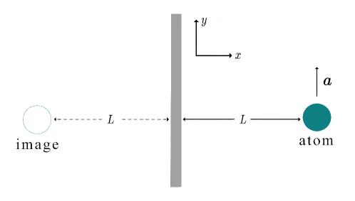
Figure 1: An atom is uniformly accelerated along the $y$-axis with a proper distance $L$ from a reflecting boundary in (2+1)-dimensional flat spacetime.

By the method of images Birrell:1984 , one can obtain the Wightman function for vacuum massless scalar fields in (2+1)-dimensional Minkowski spacetime with the presence of the reflecting boundary

$$G^{+}_{BD}(x(\tau),x(\tau^{\prime}))= \langle 0|\phi^{f}(x)\phi^{f}(x^{\prime})|0\rangle$$

$$= \frac{1}{4\pi}\frac{1}{\sqrt{\big{(}x-x^{\prime}\big{)}^{2}+\big{(}y-y^{\prime}\big{)}^{2}-\big{(}t-t^{\prime}-i\epsilon\big{)}^{2}}}$$

$$-\frac{1}{4\pi}\frac{1}{\sqrt{\big{(}x+x^{\prime}\big{)}^{2}+\big{(}y-y^{\prime}\big{)}^{2}-\big{(}t-t^{\prime}-i\epsilon\big{)}^{2}}}\;.$$ (22)

Substituting the spacetime trajectory (21) of the two-level atom into Eq. (III), we have

$$G^{+}_{BD}(x(\tau),x(\tau^{\prime}))=\frac{a}{8\pi}\frac{1}{\sqrt{-\big{[}\sinh\big{(}\frac{a\Delta\tau}{2}-i\epsilon\big{)}\big{]}^{2}}}-\frac{a}{8\pi}\frac{1}{\sqrt{-\big{[}\sinh\big{(}\frac{a\Delta\tau}{2}-i\epsilon\big{)}\big{]}^{2}+(aL)^{2}}}\;$$ (23)

with $\Delta\tau=\tau-\tau^{\prime}$.

Now we will calculate the corrections to the Lamb shift because of the presence of the boundary and acceleration. That is, what we actually calculate is the Lamb shift relative to that when the atom is at rest in a free space. In (3+1)-dimensional spacetime, directly calculating the relative Lamb shift instead of the total one avoids the tricky issue of regularizing the Lamb shift in free space. Normally, in a non-relativistic quantum field theoretic approach such as what we are using here, a suitable cutoff is needed in the regularization. However, let us note that no regularization is actually required for the (2+1)-dimensional case, as now the Lamb shift in free space is finite. Nevertheless, since our main concern in the present paper is the corrections due to the boundary and acceleration here and the BTZ spacetime later, we only examine the relative Lamb shift.

So, in our calculation of the atomic energy-level shifts, we shall use the Wightman function $G^{+R}_{BD}(x(\tau),x(\tau^{\prime}))$ which is obtained by subtracting from the Wightman function (23) that of the massless scalar field in the Minkowski vacuum in (2+1)-dimensional flat spacetime given by Takagi:1986

$$G^{+}_{FLA}(x(\tau),x(\tau^{\prime}))=\frac{1}{4\pi\sqrt{(x-x^{\prime})^{2}+(y-y^{\prime})^{2}-(t-t^{\prime}-i\varepsilon)^{2}}}=\frac{1}{4\pi\sqrt{-(\Delta\tau-i\varepsilon)^{2}}}\;$$ (24)

to give

$$G^{+R}_{BD}(x(\tau),x(\tau^{\prime}))=G^{+}_{BD}(x(\tau),x(\tau^{\prime}))-G^{+}_{FLA}(x(\tau),x(\tau^{\prime}))\;.$$ (25)

Then, two statistical functions of the field can be written as the symmetrized and anti-symmetrized Wightman functions:

$$C^{F}_{BD}(x(\tau),x(\tau^{\prime}))=\frac{1}{2}\big{[}G^{+R}_{BD}(x(\tau),x(\tau^{\prime}))+G^{+R}_{BD}(x(\tau^{\prime}),x(\tau))\big{]}\;,$$ (26)

$$\chi^{F}_{BD}(x(\tau),x(\tau^{\prime}))=\frac{1}{2}\big{[}G^{+R}_{BD}(x(\tau),x(\tau^{\prime}))-G^{+R}_{BD}(x(\tau^{\prime}),x(\tau))\big{]}\;.$$ (27)

Substituting the above statistical functions into Eqs. (16) and (17), we can separately calculate the contributions of vacuum fluctuations and radiation reaction to the energy shift of level $b$. Generally, it is difficult to directly compute the integrals involved by using the residual theorem and the contour integration technique. So, we now first write the statistical functions as the following Fourier integrals

$$C^{F}_{BD}(x(\tau),x(\tau^{\prime}))=\frac{1}{4\pi}\int_{-\infty}^{\infty}\big{[}e^{i\omega(\tau-\tau^{\prime})}F^{R}_{BD}(\omega)+e^{-i\omega(\tau-\tau^{\prime})}F^{R}_{BD}(\omega)\big{]}d\omega\;,$$ (28)

$$\chi^{F}_{BD}(x(\tau),x(\tau^{\prime}))=\frac{1}{4\pi}\int_{-\infty}^{\infty}\big{[}e^{i\omega(\tau-\tau^{\prime})}F^{R}_{BD}(\omega)-e^{-i\omega(\tau-\tau^{\prime})}F^{R}_{BD}(\omega)\big{]}d\omega\;,$$ (29)

where $F^{R}_{BD}(\omega)$ represents the Fourier transform of the Wightman function $G_{BD}^{+R}(\Delta\tau)$, that is

$$F^{R}_{BD}(\omega):=\int_{-\infty}^{+\infty}G_{BD}^{+R}(\Delta\tau)e^{-i\omega\Delta\tau}d\Delta\tau=F_{BD}(\omega)-F_{FLA}(\omega)\;.$$ (30)

Here, the Fourier transform of the Wightman function $G_{BD}^{+}(\Delta\tau)$, which is actually the response function of a uniformly accelerated particle detector near the reflecting boundary, takes the following form (see Appendix A for details)

$$F_{BD}(\omega)=\frac{1}{2}\frac{1}{e^{\omega/T_{u}}+1}\Big{[}1-P_{\frac{i\omega}{2\pi T_{u}}-\frac{1}{2}}\big{(}8\pi^{2}T_{u}^{2}L^{2}+1\big{)}\Big{]}\;$$ (31)

with the Unruh temperature $T_{u}=a/2\pi$, and $P_{\nu}(x)$ representing the associated Legendre function of the first kind Gradshteyn:2007

$$P_{\nu}(\cosh\alpha):=\frac{\sqrt{2}}{\pi}\int_{0}^{\alpha}\frac{\cosh[(\nu+\frac{1}{2})u]}{(\cosh\alpha-\cosh u)^{\frac{1}{2}}}du,\quad\alpha>0\;,$$ (32)

while the Fourier transform of Eq. (24) can be straightforwardly carried out as

$$F_{FLA}(\omega)=\int_{-\infty}^{+\infty}G_{FLA}^{+}(\Delta\tau)e^{-i\omega\Delta\tau}d\Delta\tau=\frac{1}{2}\theta(-\omega)\;$$ (33)

with $\theta(x)$ representing the Heaviside step function. Thus, we have

$$F^{R}_{BD}(\omega)=\frac{1}{2}\frac{1}{e^{\omega/T_{u}}+1}-\frac{1}{2}\frac{1}{e^{\omega/T_{u}}+1}P_{\frac{i\omega}{2\pi T_{u}}-\frac{1}{2}}\big{(}8\pi^{2}T_{u}^{2}L^{2}+1\big{)}-\frac{\theta(-\omega)}{2}\;.$$ (34)

As we can see that the first, the second and the third term in $F^{R}_{BD}(\omega)$ respectively originates from the first, the second term in Eq. (23) and the Fourier transform of the Wightman function of the static atom, and therefore they respectively correspond to terms associated with the accelerated atom, the image of it and the static atom. A substitution of Eq. (34) into Eq. (28) yields the symmetric correlation function for the field

$$C^{F}_{BD}(x(\tau),x(\tau^{\prime}))=-\frac{1}{8\pi}\int_{0}^{\infty}d\omega\big{(}e^{{i}\omega{\Delta\tau}}+e^{{-i}\omega{\Delta\tau}}\big{)}P_{\frac{i\omega}{2\pi T_{u}}-\frac{1}{2}}\big{(}8\pi^{2}T_{u}^{2}L^{2}+1\big{)}\;,$$ (35)

where the identity $P_{\nu}(x)=P_{-\nu-1}(x)$ has been used. Here, the integration of $F_{FLA}(\omega)$ cancels out that over the first term of $F^{R}_{BD}(\omega)$, i.e., $(2e^{\omega/T_{u}}+2)^{-1}$ in Eq. (34). Similarly, the linear susceptibility function of the field works out to

$$\chi^{F}_{BD}(x(\tau),x(\tau^{\prime}))= -\frac{1}{8\pi}\int_{0}^{\infty}d\omega\Big{(}e^{{i}\omega{\Delta\tau}}-e^{{-i}\omega{\Delta\tau}}\Big{)}\Big{\{}\tanh\Big{(}\frac{\omega}{2T_{u}}\Big{)}$$

$$\times\Big{[}1-P_{\frac{i\omega}{2\pi T_{u}}-\frac{1}{2}}\big{(}8\pi^{2}T_{u}^{2}L^{2}+1\big{)}\Big{]}-1\Big{\}}\;.$$ (36)

Inserting above equations into Eqs. (16) and (17) and extending the range of integration to infinity for sufficiently long time interval, the contributions of vacuum fluctuations and radiation reaction to the energy shift of the level state $|b\rangle$ ($b\in\{-,+\}$) are found to be respectively given by

$$(\delta E_{b})_{vf}= -\frac{\mu^{2}}{8\pi}\sum_{d}\big{|}\big{\langle}b\big{|}R_{2}(0)\big{|}d\big{\rangle}\big{|}^{2}\int_{0}^{\infty}d\omega{\mathcal{P}}\Big{(}\frac{1}{\omega+\omega_{bd}}-\frac{1}{\omega-\omega_{bd}}\Big{)}$$

$$\times P_{\frac{i\omega}{2\pi T_{u}}-\frac{1}{2}}\big{(}8\pi^{2}T_{u}^{2}L^{2}+1\big{)}\;,$$ (37)

$$(\delta E_{b})_{rr}= -\frac{\mu^{2}}{8\pi}\sum_{d}\big{|}\big{\langle}b\big{|}R_{2}(0)\big{|}d\big{\rangle}\big{|}^{2}\int_{0}^{\infty}d\omega{\mathcal{P}}\Big{(}\frac{1}{\omega+\omega_{bd}}+\frac{1}{\omega-\omega_{bd}}\Big{)}$$

$$\times\Big{\{}\tanh\Big{(}\frac{\omega}{2T_{u}}\Big{)}\Big{[}1-P_{\frac{i\omega}{2\pi T_{u}}-\frac{1}{2}}\big{(}8\pi^{2}T_{u}^{2}L^{2}+1\big{)}\Big{]}-1\Big{\}}\;,$$ (38)

where $\mathcal{P}$ denotes the principal value integral. It follows from Eqs. (III) and (III) that $(\delta E_{+})_{vf}=-(\delta E_{-})_{vf}$ and $(\delta E_{+})_{rr}=(\delta E_{-})_{rr}$. So, the Lamb shift for the accelerated atom near the reflecting boundary is determined by $(\delta E_{+})_{vf}$ only, and it is given, after considering $\sum\limits_{d}|\langle b|R_{2}(0)|d\rangle|^{2}=1/4$, by

$$\Delta_{BD}=-\frac{\mu^{2}}{16\pi}\int_{0}^{\infty}d\omega{\mathcal{P}}\Big{(}\frac{1}{\omega+\omega_{0}}-\frac{1}{\omega-\omega_{0}}\Big{)}P_{\frac{i\omega}{2\pi T_{u}}-\frac{1}{2}}\big{(}8\pi^{2}T_{u}^{2}L^{2}+1\big{)}\;.$$ (39)

It is interesting to note that here only the contribution from the image of accelerated atom retains, and the contribution from the accelerated atom cancels that of the static atom, meaning that uniform acceleration does not induce corrections to the Lamb shift in free space without boundary. Furthermore, from the following properties of the associated Legendre function of the first kind,

$$\lim_{x\rightarrow\infty}P_{iy-1/2}(x^{2}+1)=0,~{}~{}y\in\rm{Reals}\;$$ (40)

and

$$\lim_{y\rightarrow\infty}P_{iy-1/2}(x^{2}+1)=0,~{}~{}x\neq 0\;,$$ (41)

we can see that $\Delta_{BD}$ vanishes when $L\rightarrow\infty$ which means there is no the correction to the Lamb shift of the accelerated atom in a free space in (2+1)-dimensional spacetime. So does the result in the limit of $a\rightarrow\infty$ (or $T_{u}\rightarrow\infty$) for a finite distance $L$, meaning that the corrections to the Lamb shift near a reflecting boundary approach zero as acceleration grows extremely large.

IV The Lamb shift for a static atom in the BTZ spacetime

In this section, we consider the Lamb shift for a static two-level atom coupled to conformal massless scalar fields in vacuum in the BTZ spacetime of which the line element can be written in Schwarzschild-like coordinates Lifschytz:1994 ; Carlip:1995 as

$$ds^{2}=-\frac{r^{2}-M\ell^{2}}{\ell^{2}}dt^{2}+\frac{\ell^{2}}{r^{2}-M\ell^{2}}dr^{2}+r^{2}d\phi^{2}\;.$$ (42)

The metric describes an asymptotically anti-de Sitter space with $\Lambda=-1/\ell^{2}$ a negative cosmological constant, which has a horizon at $r_{+}=\sqrt{M}\ell$ with $M$ representing the mass of the BTZ solution.

To obtain the Lamb shift in the BTZ spacetime, we need the Wightman function of the conformal scalar field to evaluate the contributions of vacuum fluctuations and radiation reaction to the atomic energy level shifts. In this paper, we assume that the scalar field is in the Hartle-Hawking vacuum in the BTZ spacetime. Note that since the BTZ spacetime can be obtained by a topological identification of $AdS_{3}$ spacetime, the Wightman function for the conformal massless scalar field in the Hartle-Hawking vacuum in the BTZ spacetime can be expressed in terms of the corresponding Wightman function in $AdS_{3}$ spacetime by using the method of images Lifschytz:1994 ; Carlip:1995

$$G^{+}_{BTZ}(x,x^{\prime})=\sum_{n=-\infty}^{+\infty}G^{+}_{AdS}(x,\Gamma^{n}{x}^{\prime})\;,$$ (43)

where $G^{+}_{AdS}(x,{x}^{\prime})$ is the Wightman function in $AdS_{3}$ spacetime and $\Gamma{x}^{\prime}$ represents the action of the identification $\phi\mapsto\phi+2\pi$ on point $x^{\prime}$. Assuming, for simplicity, that the field satisfies the Dirichlet boundary condition at spatial infinity due to lack of global hyperbolicity of the BTZ spacetime, the Wightman function can be found analytically as follows Lifschytz:1994

$$G^{+}_{BTZ}(x,x^{\prime})=\frac{1}{4\sqrt{2}\pi\ell}\sum_{n=-\infty}^{\infty}\left[\frac{1}{\sqrt{\sigma_{n}}}-\frac{1}{\sqrt{\sigma_{n}+2}}\right]\;,$$ (44)

where

$$\sigma_{n}:=\frac{{r}r^{\prime}}{r_{+}^{2}}\cosh\left[\sqrt{M}(\Delta\phi-2\pi n)\right]-1-\frac{\sqrt{\left(r^{2}-r_{+}^{2}\right)\left(r^{\prime 2}-r_{+}^{2}\right)}}{r_{+}^{2}}\cosh\left[\frac{r_{+}}{\ell^{2}}\Delta t\right]\;,$$ (45)

with $\Delta\phi=\phi-\phi^{\prime},~{}\Delta{t}=t-t^{\prime}$.

In the following discussions, we suppose that the two-level atom is spatially fixed at a constant $r$ in the BTZ spacetime such that $\Delta\phi=0,~{}\Delta\tau=\tau-\tau^{\prime}=\sqrt{-g_{00}}\Delta{t}$. Since our interest is the relative Lamb shift in the BTZ spacetime, we shall use the Wightman function which is obtained by subtracting that in the Minkowski vacuum in (2+1)-dimensional flat spacetime in the subsequent discussions, i.e., $G_{BTZ}^{+R}(\Delta\tau):=G_{BTZ}^{+}(\Delta\tau)-G_{FLA}^{+}(\Delta\tau)$. Then the Fourier transform for the Wightman function $G_{BTZ}^{+R}(\Delta\tau)$ reads

$$F^{R}_{BTZ}(\omega):=\int_{-\infty}^{+\infty}G_{BTZ}^{+R}(\Delta\tau)e^{-i\omega\Delta\tau}d\Delta\tau=F_{BTZ}(\omega)-F_{FLA}(\omega)\;.$$ (46)

Note that $F_{FLA}(\omega)$ is given by Eq. (33). Here, the Fourier transform of the Wightman function (44), $F_{BTZ}(\omega)$, along the trajectory of the static atom is given by Lifschytz:1994 , which is the response function of a static detector in the BTZ spacetime as well

$$F_{BTZ}(\omega)= \int_{-\infty}^{+\infty}G_{BTZ}^{+}(\Delta\tau)e^{-i\omega\Delta\tau}d\Delta\tau$$

$$= \frac{1}{2}\frac{1}{e^{\omega/T_{h}}+1}\sum_{n=-\infty}^{\infty}\Big{[}P_{\frac{i\omega}{2\pi T_{h}}-\frac{1}{2}}(\cosh\alpha_{n})-P_{\frac{i\omega}{2\pi T_{h}}-\frac{1}{2}}(\cosh\beta_{n})\Big{]}\;,$$ (47)

where $T_{h}$ is the local temperature given by

$$T_{h}=\frac{r_{+}}{2\pi\ell\sqrt{r^{2}-r_{+}^{2}}}\;,$$ (48)

and the auxiliary functions $\cosh\alpha_{n}$ and $\cosh\beta_{n}$ are defined as

$$\cosh\alpha_{n}:=\frac{r_{+}^{2}}{r^{2}-r_{+}^{2}}\Big{[}\frac{r^{2}}{r_{+}^{2}}\cosh\Big{(}2\pi{n}\sqrt{M}\Big{)}-1\Big{]}\;,$$

$$\cosh\beta_{n}:=\frac{r_{+}^{2}}{r^{2}-r_{+}^{2}}\Big{[}\frac{r^{2}}{r_{+}^{2}}\cosh\Big{(}2\pi{n}\sqrt{M}\Big{)}+1\Big{]}\;.$$ (49)

Let us note that the local temperature of the BTZ spacetime can be rewritten in the following form Zhjl:2020

$$T_{h}=\frac{\sqrt{a_{BTZ}^{2}-\ell^{-2}}}{2\pi}\;$$ (50)

with $a_{BTZ}:=r/(\ell\sqrt{r^{2}-r_{+}^{2}})$ representing the acceleration of the constant $r$ trajectory in the BTZ spacetime. Here $T_{h}$ is analogous to the temperature felt by an accelerated observer in $AdS_{3}$ spacetime Jennings:2010 . It is demonstrated in Ref. Jennings:2010 that there exists a critical acceleration, $1/\ell$, in $AdS_{3}$ spacetime, and only the observer with a constant super-critical acceleration $a$ (i.e., $a>1/\ell$) can register the quasi-thermal response with a temperature equal to $\sqrt{a^{2}-\ell^{-2}}/(2\pi)$. Noteworthily, the response function (IV) displays the Fermi-Dirac distribution as was noted in Ref. Lifschytz:1994 .

Consequently, we can reexpress the Fourier transform of the Wightman function $G^{+R}_{BD}(x(\tau),x(\tau^{\prime}))$ as

$$F^{R}_{BTZ}(\omega)=F^{R}_{n=0}(\omega)+F^{R}_{n\neq 0}(\omega)$$ (51)

with

$$F^{R}_{n=0}(\omega)=\frac{1}{2}\frac{1}{e^{\omega/T_{h}}+1}-\frac{1}{2}\frac{1}{e^{\omega/T_{h}}+1}P_{\frac{i\omega}{2\pi T_{h}}-\frac{1}{2}}(\cosh\beta_{0})-\frac{\theta(-\omega)}{2}\;,$$ (52)

and

$$F^{R}_{n\neq 0}(\omega)=\frac{1}{e^{\omega/T_{h}}+1}\sum_{n=1}^{\infty}\Big{[}P_{\frac{i\omega}{2\pi T_{h}}-\frac{1}{2}}(\cosh\alpha_{n})-P_{\frac{i\omega}{2\pi T_{h}}-\frac{1}{2}}(\cosh\beta_{n})\Big{]}\;,$$ (53)

where we have used the identity $P_{\nu}(1)=1$ for the associated Legendre function of the first kind and split $F^{R}_{BTZ}(\omega)$ into $n=0$ and $n\neq 0$ terms for convenience.

With the symmetric correlation function defined in (14), we have

$$C^{F}_{BTZ}(x(\tau),x(\tau^{\prime}))= \frac{1}{4\pi}\sum_{n=1}^{\infty}\int_{0}^{\infty}d\omega\Big{(}e^{{i}\omega{\Delta\tau}}+e^{{-i}\omega{\Delta\tau}}\Big{)}\Big{[}P_{\frac{i\omega}{2\pi T_{h}}-\frac{1}{2}}\left(\cosh\alpha_{n}\right)-P_{\frac{i\omega}{2\pi T_{h}}-\frac{1}{2}}(\cosh\beta_{n})\Big{]}$$

$$-\frac{1}{8\pi}\int_{0}^{\infty}d\omega\Big{(}e^{{i}\omega{\Delta\tau}}+e^{{-i}\omega{\Delta\tau}}\Big{)}P_{\frac{i\omega}{2\pi T_{h}}-\frac{1}{2}}(\cosh\beta_{0})\;.$$ (54)

One can see from Eq. (IV) that the inverse-Fourier integration over $F_{FLA}(\omega)$ also cancels out that over the first term in $F^{R}_{n=0}(\omega)$, i.e., $(2e^{\omega/T_{h}}+2)^{-1}$ in Eq. (52). Similarly, the linear susceptibility function takes the following form

$$\chi^{F}_{BTZ}(x(\tau),x(\tau^{\prime}))= -\frac{1}{4\pi}\sum_{n=1}^{\infty}\int_{0}^{\infty}d\omega\Big{(}e^{{i}\omega{\Delta\tau}}-e^{{-i}\omega{\Delta\tau}}\Big{)}\tanh\Big{(}\frac{\omega}{2T_{h}}\Big{)}\Big{[}P_{\frac{i\omega}{2\pi{T_{h}}}-\frac{1}{2}}(\cosh\alpha_{n})$$

$$-P_{\frac{i\omega}{2\pi T_{h}}-\frac{1}{2}}(\cosh\beta_{n})\Big{]}-\frac{1}{8\pi}\int_{0}^{\infty}d\omega\Big{(}e^{{i}\omega{\Delta\tau}}-e^{{-i}\omega{\Delta\tau}}\Big{)}\Big{\{}\tanh\Big{(}\frac{\omega}{2T_{h}}\Big{)}$$

$$\times\Big{[}1-P_{\frac{i\omega}{2\pi T_{h}}-\frac{1}{2}}(\cosh\beta_{0})\Big{]}-1\Big{\}}\;.$$ (55)

Inserting above equations into Eqs. (16) and (17), the contributions of vacuum fluctuations and radiation reaction to the energy shift of the level state $|b\rangle$ are found to be respectively given by

$$(\delta E_{b})_{vf}= \frac{\mu^{2}}{4\pi}\sum\limits_{d}|\langle b|R_{2}(0)|d\rangle|^{2}\sum_{n=1}^{\infty}\int_{0}^{\infty}d\omega{\mathcal{P}}\Big{(}\frac{1}{\omega+\omega_{bd}}-\frac{1}{\omega-\omega_{bd}}\Big{)}\Big{[}P_{\frac{i\omega}{2\pi{T_{h}}}-\frac{1}{2}}(\cosh\alpha_{n})$$

$$-P_{\frac{i\omega}{2\pi{T_{h}}}-\frac{1}{2}}(\cosh\beta_{n})\Big{]}-\frac{\mu^{2}}{8\pi}\sum\limits_{d}|\langle b|R_{2}(0)|d\rangle|^{2}\int_{0}^{\infty}d\omega{\mathcal{P}}\Big{(}\frac{1}{\omega+\omega_{bd}}-\frac{1}{\omega-\omega_{bd}}\Big{)}$$

$$\times P_{\frac{i\omega}{2\pi{T_{h}}}-\frac{1}{2}}(\cosh\beta_{0})\;,$$ (56)

and

$$(\delta E_{b})_{rr}= -\frac{\mu^{2}}{4\pi}\sum\limits_{d}|\langle b|R_{2}(0)|d\rangle|^{2}\sum_{n=1}^{\infty}\int_{0}^{\infty}d\omega{\mathcal{P}}\Big{(}\frac{1}{\omega+\omega_{bd}}+\frac{1}{\omega-\omega_{bd}}\Big{)}\tanh\Big{(}\frac{\omega}{2T_{h}}\Big{)}$$

$$\times\Big{[}P_{\frac{i\omega}{2\pi{T_{h}}}-\frac{1}{2}}(\cosh\alpha_{n})-P_{\frac{i\omega}{2\pi{T_{h}}}-\frac{1}{2}}(\cosh\beta_{n})\Big{]}-\frac{\mu^{2}}{8\pi}\sum\limits_{d}|\langle b|R_{2}(0)|d\rangle|^{2}$$

$$\times\int_{0}^{\infty}d\omega{\mathcal{P}}\Big{(}\frac{1}{\omega+\omega_{bd}}+\frac{1}{\omega-\omega_{bd}}\Big{)}\Big{\{}\tanh\Big{(}\frac{\omega}{2T_{h}}\Big{)}\Big{[}1-P_{\frac{i\omega}{2\pi{T_{h}}}-\frac{1}{2}}(\cosh\beta_{0})\Big{]}-1\Big{\}}\;.$$ (57)

So, it is easy to get that the Lamb shift for the two-level atom in the BTZ spacetime is determined by $(\delta E_{+})_{vf}$ only, that is

$$\Delta_{BTZ}=2(\delta E_{+})_{vf}= \Delta_{n=0}+\Delta_{n\neq 0}\;$$ (58)

with

$$\Delta_{n=0}:= -\frac{\mu^{2}}{16\pi}\int_{0}^{\infty}d\omega{\mathcal{P}}\Big{(}\frac{1}{\omega+\omega_{0}}-\frac{1}{\omega-\omega_{0}}\Big{)}P_{\frac{i\omega}{2\pi T_{h}}-\frac{1}{2}}(\cosh\beta_{0})$$

$$= -\frac{\mu^{2}}{16\pi}\int_{0}^{\infty}d\omega{\mathcal{P}}\Big{(}\frac{1}{\omega+\omega_{0}}-\frac{1}{\omega-\omega_{0}}\Big{)}P_{\frac{i\omega}{2\pi T_{h}}-\frac{1}{2}}\big{(}8\pi^{2}T_{h}^{2}\ell^{2}+1\big{)}\;,$$ (59)

and

$$\Delta_{n\neq 0}:=\frac{\mu^{2}}{8\pi}\sum_{n=1}^{\infty}\int_{0}^{\infty}d\omega{\mathcal{P}}\Big{(}\frac{1}{\omega+\omega_{0}}-\frac{1}{\omega-\omega_{0}}\Big{)}\Big{[}P_{\frac{i\omega}{2\pi T_{h}}-\frac{1}{2}}(\cosh\alpha_{n})-P_{\frac{i\omega}{2\pi T_{h}}-\frac{1}{2}}(\cosh\beta_{n})\Big{]}\;.$$ (60)

Here $\Delta_{n=0}$ represents the contribution from the second term of the response function $F^{R}_{n=0}(\omega)$ in (51), and $\Delta_{n\neq 0}$ results from $F^{R}_{n\neq 0}(\omega)$.

Recalling the Lamb shift of the accelerated atom near the reflecting boundary, $\Delta_{BD}$ (i.e., Eq. (39)), we find that Eqs. (39) and  (IV) become the same if one replaces $T_{u}$ and $L$ in Eq. (39) with $T_{h}$ and $\ell$ (or equivalently, let $a\equiv\sqrt{a_{BTZ}^{2}-\ell^{-2}}$ and $L\equiv\ell$). In fact, this equivalence between $\Delta_{n=0}$ and $\Delta_{BD}$ can also be seen from the response functions, since the $n=0$ term in the response function (IV) in the BTZ spacetime, i.e.,

$$\frac{1}{2}\frac{1}{e^{\omega/T_{h}}+1}\Big{[}1-P_{\frac{i\omega}{2\pi T_{h}}-\frac{1}{2}}(8\pi^{2}T_{h}^{2}\ell^{2}+1)\Big{]}\;,$$ (61)

coincides with Eq. (31).

Let us now analyze the contribution of $n\neq 0$ terms in the response function to the Lamb shift. Considering that the auxiliary functions in Eq. (IV) can be rewritten as

$$\cosh\alpha_{n}=8\pi^{2}T_{h}^{2}{r^{2}\sinh^{2}\big{(}n\pi\sqrt{M}\big{)}}/{M}+1\;,$$

$$\cosh\beta_{n}=8\pi^{2}T_{h}^{2}\Big{[}{\frac{r^{2}}{M}\sinh^{2}\big{(}n\pi\sqrt{M}\big{)}}+\ell^{2}\Big{]}+1\;,$$ (62)

we have

$$\Delta_{n\neq 0}= \frac{\mu^{2}}{8\pi}\sum_{n=1}^{\infty}\;\Bigg{[}\int_{0}^{\infty}d\omega{\mathcal{P}}\Big{(}\frac{1}{\omega+\omega_{0}}-\frac{1}{\omega-\omega_{0}}\Big{)}P_{\frac{i\omega}{2\pi T_{h}}-\frac{1}{2}}(8\pi^{2}T_{h}^{2}L_{\alpha_{n}}^{2}+1)$$

$$-\int_{0}^{\infty}d\omega{\mathcal{P}}\Big{(}\frac{1}{\omega+\omega_{0}}-\frac{1}{\omega-\omega_{0}}\Big{)}P_{\frac{i\omega}{2\pi T_{h}}-\frac{1}{2}}(8\pi^{2}T_{h}^{2}L_{\beta_{n}}^{2}+1)\Bigg{]}\;$$ (63)

with $L_{\alpha_{n}}:={r\sinh\big{(}n\pi\sqrt{M}\big{)}}/\sqrt{M}$ and $L_{\beta_{n}}:=[{r^{2}\sinh^{2}\big{(}n\pi\sqrt{M}\big{)}}/{M}+\ell^{2}]^{1/2}$. A comparison of the above result with Eq. (39) suggests that the contribution of each ${n\neq 0}$ term to the Lamb shift can be understood as that from a pair of a source, which is accelerated along a reflecting boundary at an effective distance to $L_{\alpha_{n}}$ in a flat spacetime with an acceleration $a=2\pi{T_{h}}=\sqrt{a_{BTZ}^{2}-\ell^{-2}}=\sqrt{M/(r^{2}-M\ell^{2})}$, and an image with the same acceleration but at a different effective distance $L_{\beta_{n}}$.

Now, let us turn our attention to analytically evaluating the Lamb shift $\Delta_{BTZ}$ in some special cases. First, for the case of the atom in the asymptotic region far form the horizon, i.e., $r\gg r_{+}$. In this case, the temperature $T_{h}$ is very small while both $T_{h}^{2}L_{\alpha_{n}}^{2}$ and $T_{h}^{2}L_{\beta_{n}}^{2}$ approach $\sinh^{2}(n\pi\sqrt{M})/(4\pi^{2})$, and then according to Eq. (41), we only need to take $\Delta_{n=0}$ into account, which is now given by (see Appendix B for details)

$$\Delta_{BTZ}\approx\Delta_{n=0}\approx-\frac{\mu^{2}}{16}\Big{[}H_{0}(2\omega_{0}\ell)-\frac{r_{+}^{2}}{r^{2}}f(2\omega_{0}\ell)\Big{]}\;,$$ (64)

with

$$f(2\omega_{0}\ell)=\frac{1}{12\omega_{0}\ell}\Big{[}4\omega_{0}^{2}\ell^{2}H_{-1}(2\omega_{0}\ell)+4\omega_{0}\ell H_{0}(2\omega_{0}\ell)-H_{1}(2\omega_{0}\ell)\Big{]}\;,$$ (65)

which can be further expressed, in the limit of $r\rightarrow\infty$ (or $a_{BTZ}\rightarrow 1/\ell$) as

$$\Delta_{BTZ}=-\frac{\mu^{2}}{16}H_{0}(2\omega_{0}\ell)\approx\left\{\begin{aligned} &-\frac{\mu^{2}\omega_{0}\ell}{4\pi}\;,\quad&\omega_{0}\ell\ll 1\;;\\ &-\frac{\mu^{2}}{16\sqrt{\pi\omega_{0}\ell}}\sin\Big{(}2\omega_{0}\ell-\frac{\pi}{4}\Big{)}\;,\quad&\omega_{0}\ell\gg 1\;.\end{aligned}\right.$$ (66)

It is worthwhile to note that $\Delta_{BTZ}$ in the asymptotic region is negative when $\omega_{0}\ell\ll 1$ or $\ell/\lambda_{0}\ll 1$. Here $\lambda_{0}:=1/\omega_{0}$ denotes the transition wavelength of the atom. This means that the Lamb shift is always suppressed in the BTZ spacetime, while it can be either positive or negative when $\omega_{0}\ell\gg 1$ or $\ell/\lambda_{0}\gg 1$, signaling either enhancement or suppression contingent on the value of $\omega_{0}\ell$.

When the atom is in the region near the horizon of the BTZ spacetime, i.e., ${r-r_{+}}\ll{r_{+}}$, since both $L_{\alpha_{n}}$ and $L_{\beta_{n}}$ are finite and the temperature $T_{h}$ is extremely large, $\Delta_{n\neq 0}$ is also negligible. So again, only $\Delta_{n=0}$ needs to be considered for the Lamb shift, which can now be approximated as (see Appendix B for details)

$$\Delta_{BTZ}\approx-\frac{\mu^{2}\omega_{0}\ell(r-r_{+})}{16\pi r_{+}}\Big{[}\ln\Big{(}\frac{r-r_{+}}{2r_{+}}\Big{)}\Big{]}^{2}\;.$$ (67)

Interestingly, as the atom approaches the horizon, i.e., $r\rightarrow r_{+}$, the above results suggest that $\Delta_{BTZ}$ would vanish, implying that the Lamb shift reduces to that in the flat spacetime. This is remarkable since the temperature $T_{h}$ or acceleration $a_{BTZ}$ blows up as the horizon is approached.

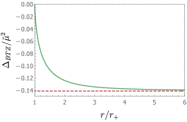
(a) $\ell/\lambda_{0}=0.05$

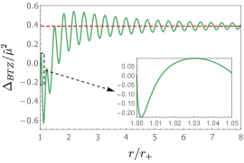
(b) $\ell/\lambda_{0}=6.00$

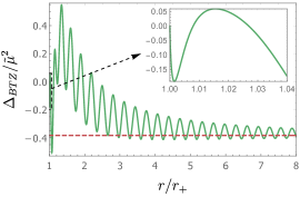
(c) $\ell/\lambda_{0}=7.00$

Figure 2: The Lamb shift is plotted as a function of $r/r_{+}$ for (a) $\ell/\lambda_{0}=0.05$, (b) $\ell/\lambda_{0}=6.00$, (c) and $\ell/\lambda_{0}=7.00$ with the transition wavelength of the atom defined by $\lambda_{0}=1/\omega_{0}$. Here, we have taken $\tilde{\mu}^{2}={\mu^{2}}/{(8\sqrt{2}\pi)}$ and $M=0.20$. The dashed red lines in all plots indicate the corresponding convergent values of $\Delta_{BTZ}/\tilde{\mu}^{2}$ (i.e., approximately equal to $-0.1413$ in (a), $0.3833$ in (b), and $-0.3831$ in (c)) in the limit of $r\rightarrow\infty$.

We now examine the properties of the Lamb shift at a generic spatial position $r$. We will resort to numerical calculation since exact analytical results are unobtainable. In Fig. (2), the Lamb shift is plotted as a function of the spatial position $r/r_{+}$ with given mass $M$ and $\ell/\lambda_{0}$. As shown in Fig. (2), the Lamb shift approaches a fixed value, i.e., $-\mu^{2}H_{0}(2\ell/\lambda_{0})/16$, in the asymptotic region of the BTZ spacetime, which is always negative for $\ell/\lambda_{0}\ll 1$ (see Fig. (2a)) but can be either positive or negative for $\ell/\lambda_{0}\gg 1$ depending on the value of $\ell/\lambda_{0}$ (see Fig. (2b) (2c)). This is in agreement with our previous results obtained by analytical analysis in Eq. (66). Moreover, at $r/r_{+}\sim 1$, all plots in Fig. (2) reveal a vanishing Lamb shift, and this is again in accordance with our analytical result (Eq. (67)) very close to the horizon.

Notably, Fig. (2a) also indicates that the Lamb shift is always suppressed in the BTZ spacetime as compared to that in the flat spacetime as long as $\ell/\lambda_{0}\ll 1$, i.e., when the transition wavelength of the atom is much larger than the $AdS$ radius of the BTZ spacetime, not just in the asymptotic region as our analytical result may seem to suggest. However, if the atomic transition wavelength is much less than the $AdS$ radius, i.e., $\ell/\lambda_{0}\gg 1$, the Lamb shift exhibits obvious oscillations as the atom is moved away from the horizon. Moreover, Fig. (2b) shows that, for a given value of $\ell/\lambda_{0}$ that gives a positive asymptotic Lamb shift, the Lamb shift may be significantly suppressed with a few oscillations in the vicinity of the horizon as compared to that in the flat spacetime and oscillates around the positive asymptotic value as the atom is moved far away from the horizon of the BTZ spacetime, while Fig. (2c) demonstrates that, for a given value of $\ell/\lambda_{0}$ that leads to a negative asymptotic Lamb shift, the Lamb shift may instead be significantly enhanced with a few oscillations in the vicinity of the horizon as compared to that in the flat spacetime and oscillates around the negative asymptotic value. Finally, let us note that the qualitative behaviors of the Lamb shift are not very sensitive of the value of $M$ which is dimensionless in the BTZ spacetime. So, a value of 0.2 is chosen in our plots of numerical computations.

V Conclusion

We have studied the Lamb shift of a two-level atom arising from its coupling to the conformal massless scalar field, which satisfies the Dirichlet boundary conditions, in the Hartle-Hawking vacuum in the BTZ spacetime, and compared it with that of the uniformly accelerated atom near a perfectly reflecting boundary in the (2+1)-dimensional flat spacetime.

We demonstrate that, for a spatially fixed atom in the BTZ spacetime, its Lamb shift is structurally similar to that of a uniformly accelerated atom near a perfectly reflecting boundary in the (2+1)-dimensional flat spacetime with an acceleration $a=2\pi T_{h}$ where $T_{h}$ is the local temperature of the BTZ spacetime. Both analytical analysis and numerical computation show that the Lamb shift is suppressed in the BTZ spacetime as compared to that in the flat spacetime as long as the transition wavelength of the atom is much larger than the $AdS$ radius while it can be either suppressed or enhanced if the transition wavelength of the atom is much less than the $AdS$ radius. In contrast, the Lamb shift is always suppressed very close to the horizon of the BTZ spacetime and remarkably it rolls back to that in the flat spacetime as the horizon is approached although the local temperature diverges there.

Appendix A The derivation of $F_{BD}(\omega)$

According to the definition of the Fourier transform, we have

$$F_{BD}(\omega)= \int_{-\infty}^{+\infty}G_{BD}^{+}(\Delta\tau)e^{-i\omega\Delta\tau}d\Delta\tau$$

$$= \frac{a}{8\pi}\int_{-\infty}^{+\infty}\frac{e^{-i\omega\Delta\tau}d\Delta\tau}{\sqrt{-\big{[}\sinh\big{(}\frac{a\Delta\tau}{2}-i\epsilon\big{)}\big{]}^{2}}}-\frac{\sqrt{2}a}{8\pi}\int_{-\infty}^{+\infty}\frac{e^{-i\omega\Delta\tau}d\Delta\tau}{\sqrt{\cosh\beta_{B}-\cosh(a\Delta\tau-i\epsilon)}}\;,$$ (68)

with $\cosh{\beta_{B}}:=2a^{2}L^{2}+1$. The first integral in Eq. (A) can be obtained as follows:

$$\frac{a}{8\pi}\int_{-\infty}^{+\infty}\frac{e^{-i\omega\Delta\tau}d\Delta\tau}{\sqrt{-\big{[}\sinh\big{(}\frac{a\Delta\tau}{2}-i\epsilon\big{)}\big{]}^{2}}}$$

$$=\frac{ia}{8\pi}\int_{-\infty}^{0}e^{-i\omega\Delta\tau}\Big{|}\sinh\Big{(}\frac{a\Delta\tau}{2}-i\epsilon\Big{)}\Big{|}^{-1}d\Delta\tau-\frac{ia}{8\pi}\int_{0}^{\infty}e^{-i\omega\Delta\tau}\Big{|}\sinh\Big{(}\frac{a\Delta\tau}{2}-i\epsilon\Big{)}\Big{|}^{-1}d\Delta\tau$$

$$=\frac{a}{8\pi}\int_{-\infty}^{\infty}e^{-i\omega\Delta\tau}\Big{[}i\sinh\Big{(}\frac{a\Delta\tau}{2}\Big{)}+\epsilon\Big{]}^{-1}d\Delta\tau$$

$$=\frac{1}{2}\frac{1}{e^{2\pi\omega/a}+1}\;,$$ (69)

where in the second line an appropriate branch of the square root cut along the negative real axis has been considered via $i\epsilon$ factor (see similar treatments in Ref. Lifschytz:1994 ). Similarly, the second integral in Eq. (A) can be performed

$$-\frac{\sqrt{2}a}{8\pi}\int_{-\infty}^{+\infty}\frac{e^{-i\omega\Delta\tau}d\Delta\tau}{\sqrt{\cosh\beta_{B}-\cosh(a\Delta\tau-i\epsilon)}}$$

$$=\frac{\sqrt{2}}{8\pi i}\int_{-\infty}^{-\beta_{B}}e^{-\frac{i\omega u}{a}}(\cosh u-\cosh\beta_{B})^{-\frac{1}{2}}du-\frac{\sqrt{2}}{8\pi}\int_{-\beta_{B}}^{\beta_{B}}e^{-\frac{i\omega u}{a}}(\cosh\beta_{B}-\cosh u)^{-\frac{1}{2}}du$$

$$\quad-\frac{\sqrt{2}}{8\pi i}\int_{\beta_{B}}^{\infty}e^{-\frac{i\omega u}{a}}(\cosh u-\cosh\beta_{B})^{-\frac{1}{2}}du$$

$$=-\frac{i}{4\pi}Q_{-\frac{i\omega}{a}-\frac{1}{2}}(\cosh\beta_{B})-\frac{1}{4}P_{\frac{i\omega}{a}-\frac{1}{2}}(\cosh\beta_{B})+\frac{i}{4\pi}Q_{\frac{i\omega}{a}-\frac{1}{2}}(\cosh\beta_{B})$$

$$=-\frac{1}{2}\frac{1}{e^{2\pi\omega/a}+1}{P}_{\frac{i\omega}{a}-\frac{1}{2}}(\cosh\beta_{B})\;,$$ (70)

where $Q_{\nu}(x)$ denotes the second associated Legendre function and the identity, $Q_{\nu}(x)-Q_{-\nu-1}(x)=\pi\cot(\nu\pi)P_{\nu}(x)$, has been used in the last line. Combining Eqs. (A) and  (A), we have

$$F_{BD}(\omega)= \frac{1}{2}\frac{1}{e^{2\pi\omega/a}+1}\Big{[}1-{P}_{\frac{i\omega}{a}-\frac{1}{2}}(2a^{2}L^{2}+1)\Big{]}$$

$$= \frac{1}{2}\frac{1}{e^{\omega/T_{u}}+1}\Big{[}1-P_{\frac{i\omega}{2\pi T_{u}}-\frac{1}{2}}\big{(}8\pi^{2}T_{u}^{2}L^{2}+1\big{)}\Big{]}\;,$$ (71)

where $T_{u}=a/(2\pi)$.

Appendix B Approximations of $\Delta_{BTZ}$

Following the definition of the associated Legendre function of the first kind (32), Eq. (IV) can be rewritten as

$$\Delta_{n=0} =-\frac{\sqrt{2}\mu^{2}}{16\pi^{2}}\int_{0}^{\beta_{0}}du\int_{0}^{\infty}d\omega{\mathcal{P}}\Big{(}\frac{1}{\omega+\omega_{0}}-\frac{1}{\omega-\omega_{0}}\Big{)}\frac{\cosh\big{(}\frac{i\omega u}{2\pi T_{h}}\big{)}}{(\cosh\beta_{0}-\cosh u)^{\frac{1}{2}}}$$

$$=-\frac{\sqrt{2}\mu^{2}}{16\pi^{2}}\int_{0}^{\beta_{0}}du\int_{-\infty}^{\infty}d\omega{\mathcal{P}}\Big{(}\frac{1}{\omega+\omega_{0}}\Big{)}\frac{\cos\big{(}\frac{\omega u}{2\pi T_{h}}\big{)}}{(\cosh\beta_{0}-\cosh u)^{\frac{1}{2}}}$$

$$=-\frac{\sqrt{2}\mu^{2}\beta_{0}}{16\pi}\int_{0}^{1}ds\frac{\sin\big{(}\frac{\omega_{0}s\beta_{0}}{2\pi T_{h}}\big{)}}{\sqrt{\cosh\beta_{0}-\cosh(s\beta_{0})}}\;,$$ (72)

where we used

$$\int_{-\infty}^{\infty}d\omega\cos\Big{(}\frac{\omega u}{2\pi T_{h}}\Big{)}{\mathcal{P}}\Big{(}\frac{1}{\omega+\omega_{0}}\Big{)}=\pi\sin\Big{(}\frac{\omega_{0}u}{2\pi T_{h}}\Big{)}$$

and $s=u/\beta_{0}$ in the last line.

For the case of $r\gg{r_{+}}$, after considering $T_{h}=\sinh(\beta_{0}/2)/(2\pi\ell)$ and a power series for the integrand in Eq. (B) about small $\beta_{0}$, we have

$$\Delta_{BTZ}\approx\Delta_{n=0}= -\frac{\sqrt{2}\mu^{2}\beta_{0}}{16\pi}\int_{0}^{1}ds\frac{\sin\Big{[}\frac{\omega_{0}\ell s\beta_{0}}{\sinh(\beta_{0}/2)}\Big{]}}{\sqrt{\cosh\beta_{0}-\cosh(s\beta_{0})}}$$

$$\approx -\frac{\mu^{2}}{8\pi}\int_{0}^{1}ds\frac{\sin(2\omega_{0}\ell s)}{\sqrt{1-s^{2}}}+\frac{\mu^{2}\omega_{0}\ell\beta_{0}^{2}}{96\pi}\int_{0}^{1}ds\frac{s\cos(2\omega_{0}\ell s)}{\sqrt{1-s^{2}}}$$

$$+\frac{\mu^{2}\beta_{0}^{2}}{192\pi}\int_{0}^{1}ds\frac{(1+s^{2})\sin(2\omega_{0}\ell s)}{\sqrt{1-s^{2}}}$$

$$\approx -\frac{\mu^{2}}{16}\Big{[}H_{0}(2\omega_{0}\ell)-\frac{r_{+}^{2}}{r^{2}}f(2\omega_{0}\ell)\Big{]}\;,$$ (73)

where

$$f(2\omega_{0}\ell)=\frac{1}{12\omega_{0}\ell}\Big{[}4\omega_{0}^{2}\ell^{2}H_{-1}(2\omega_{0}\ell)+4\omega_{0}\ell H_{0}(2\omega_{0}\ell)-H_{1}(2\omega_{0}\ell)\Big{]}\;,$$ (74)

with $H_{n}(x)$ denoting the Struve function.

For the case of $({r-r_{+}})\ll{r_{+}}$, $\beta_{0}$ will be extremely large. Thus, we have

$$\Delta_{n=0}= -\frac{\sqrt{2}\mu^{2}\beta_{0}}{16\pi}\int_{0}^{1}ds\frac{\sin\big{(}\frac{\omega_{0}s\beta_{0}}{2\pi T_{h}}\big{)}}{\sqrt{\cosh\beta_{0}-\cosh(s\beta_{0})}}$$

$$\approx -\frac{\mu^{2}\beta_{0}}{16\pi}\int_{0}^{1}ds\frac{\sin\big{[}\omega_{0}s\beta_{0}/(2\pi T_{h})\big{]}}{\sinh(\beta_{0}/2)}$$

$$= -\frac{\mu^{2}T_{h}}{8\omega_{0}\sinh(\beta_{0}/2)}\Big{[}1-\cos\Big{(}\frac{\omega_{0}\beta_{0}}{2\pi T_{h}}\Big{)}\Big{]}\;.$$ (75)

According to Eq. (B), the Lamb shift can be further written as

$$\Delta_{BTZ}\approx\Delta_{n=0}\approx-\frac{\mu^{2}\omega_{0}\ell(r-r_{+})}{16\pi r_{+}}\Big{[}\ln\Big{(}\frac{r-r_{+}}{2r_{+}}\Big{)}\Big{]}^{2}\;.$$ (76)