Transonic limit of traveling waves of the Euler-Korteweg system

Abstract

We prove the convergence in the transonic limit of two-dimensional traveling waves of the E-K system, up to rescaling, toward a ground state of the Kadomtsev-Petviashvili Equation. Similarly, in dimension one we prove the convergence in the transonic limit of solitons toward the soliton of the Korteweg de Vries equation.

1 Introduction

The Euler Korteweg system, in dimension $d$, reads

$$\left\{\begin{aligned} &\partial_{t}\rho+\text{div}(\rho u)=0,\\ &\partial_{t}u+u.\nabla u+\nabla g(\rho)=\nabla\bigg{(}K(\rho)\Delta\rho+\frac{1}{2}K^{\prime}(\rho)|\nabla\rho|^{2}\bigg{)},\quad t\in\mathbb{R},\,x\in\mathbb{R}^{d},\end{aligned}\right.$$ (E-K)

where $\rho>0$ is the density of the fluid, $u\in\mathbb{R}^{d}$ is its velocity field, the right hand side of the second line is the capillary tensor. The functions $K$, $g$ are defined on $\mathbb{R}^{+}_{*}$ and smooth, the function $K$ is positive. When the velocity is irrotational i.e $u=\nabla\phi$ for some $\phi$ that cancels at infinity, the momentum equation rewrites

$$\partial_{t}\phi+\frac{|\nabla\phi|^{2}}{2}+g(\rho)=K(\rho)\Delta\rho+\frac{1}{2}K^{\prime}(\rho)|\nabla\rho|^{2}.$$

There is a formally conserved energy

$$E(\rho,\phi)=\int_{\mathbb{R}^{d}}\frac{K(\rho)|\nabla\rho|^{2}+\rho|\nabla\phi|^{2}}{2}+G(\rho)dx,$$ (1.1)

where $G$ is a primitive of $g$ with a later specified integration constant. Moreover we have a momentum

$$P(\rho,\phi)=\int_{\mathbb{R}^{d}}(\rho-\rho_{0})\partial_{1}\phi dx.$$ (1.2)

which makes sense when $\rho-\rho_{0}\in L^{2},\,\nabla\phi\in L^{2}$. The energy makes sense for $(\rho,u)$ localized near the constant state $(\rho_{0},0)$, which will be our framework. We call traveling wave a solution of (E-K) of the form

$$(\rho(x.\mathrm{n}-ct,x_{\perp}),u(x\cdot\mathrm{n}-ct,x_{\perp})),\;x_{\perp}=(x_{1},x_{2},...,x_{d})-x\cdot\mathrm{n},$$

where $c$ is the speed of propagation and $\mathrm{n}$ the direction of the speed. The direction of the speed does not matter, thus we let $\mathrm{n}=\mathrm{e_{1}}$. A traveling wave solves

$$\left\{\begin{aligned} &-c\partial_{1}\rho+\text{div}(\rho\nabla\phi)=0,\\ &-c\partial_{1}\phi+g(\rho)-K(\rho)\Delta(\rho)+\frac{|\nabla\phi|^{2}}{2}-K^{\prime}(\rho)\frac{|\nabla\rho|^{2}}{2}=0.\end{aligned}\right.$$ (1.3)

In [1], Audiard proves the existence of traveling waves in dimension two, localized near the constant state $(\rho_{0},0)$ with $g(\rho_{0})=0,\,g^{\prime}(\rho_{0})>0$. Their speed is close but less than the speed of sound that we define now. When neglecting the capilary tensor and linearizing this system near $(\rho_{0},0)$ i.e. $\rho=\rho_{0}+r$, we obtain the Euler equation

$$\left\{\begin{aligned} &\partial_{t}r+\rho_{0}\text{div}(u)=0,\\ &\partial_{t}u+g^{\prime}(\rho_{0})\nabla r=0.\end{aligned}\right.$$ (1.4)

The speed of sound is

$$c_{s}=\sqrt{\rho_{0}g^{\prime}(\rho_{0})}.$$

For simplification, we use the following rescaling

$$(\rho,\phi)=\bigg{(}\rho_{0}\rho_{r}\bigg{(}\sqrt{\frac{g^{\prime}(\rho_{0})}{\rho_{0}}x}\bigg{)},\phi_{r}\bigg{(}\sqrt{\frac{g^{\prime}(\rho_{0})}{\rho_{0}}x}\bigg{)}\bigg{)},\,K_{r}(\rho_{r})=\frac{K(\rho_{0}\rho_{r})}{\rho_{0}},$$

$$g_{r}(\rho_{r})=\frac{g(\rho_{0}\rho_{r})}{g^{\prime}(\rho_{0})\rho_{0}},c_{r}=\frac{c}{\sqrt{\rho_{0}g^{\prime}(\rho_{0})}}.$$

Then (1.3) becomes

$$\left\{\begin{aligned} &-c_{r}\partial_{1}\rho_{r}+\text{div}(\rho_{r}\nabla\phi_{r})=0,\\ &-c_{r}\partial_{1}\phi_{r}+g_{r}(\rho_{r})-K_{r}(\rho_{r})\Delta(\rho_{r})+\frac{|\nabla\phi_{r}|^{2}}{2}-K^{\prime}(\rho_{r})\frac{|\nabla\rho_{r}|^{2}}{2}=0.\end{aligned}\right.$$ (1.5)

In this system the constant state is 1, $g_{r}(1)=0$, $g_{r}^{\prime}(1)=1$ and the speed of sound is $\sqrt{1g^{\prime}(1)}=1$. We will forget the subscript $r$ and focus on the rescaled system, i.e. we will assume through the rest of the paper that

$$g(1)=0,\;g^{\prime}(1)=1\;\text{and}\;c_{s}=1.$$ (1.6)

Solutions of (1.5) with speed near the speed of sound are known to exist, the precise existence statement of [1] is the following:

Theorem 1.

([1] Theorem 1.1, proposition 3.3 and proposition 2.3) In dimension two, under the assumption $\Gamma:=3+g^{\prime\prime}(1)\neq 0$,   there exists $p_{0}>0$ such that for any $0\leq p\leq p_{0}$ we have $(\rho_{p},\phi_{p})\in\cap_{j\geq 0}\big{(}1+H^{j}\big{)}\times\dot{H}^{j+1}$, solution of $(\ref{E-K simple})$ for some $c_{p}>0$, with $P(\rho_{p},\phi_{p})=p$.
Moreover there exists $\alpha,\beta,C>0$ such that, for any $0\leq p\leq p_{0}$

$$p-\beta p^{3}\leq E(\rho_{p},\phi_{p})\leq p-\alpha p^{3},$$ (1.7)

$$1-\beta p^{2}\leq c_{p}\leq 1-\alpha p^{2},$$ (1.8)

$$||\rho_{p}-1||_{\infty}\leq C\sqrt{E(\rho_{p},\phi_{p})}\quad{\rm for}\;p\ll 1.$$ (1.9)

$$||\rho_{p}-1||_{\infty}\geq Cp^{2}\quad{\rm for}\;p\ll 1.$$ (1.10)

Remark 1.1.

As has been proven for the Schrödinger equation (see [14]), it is possible that such solitons exist in higher dimensions.

To construct the traveling waves of theorem 1 the author in [1] solves a minimization problem. On the space $\mathcal{H}=\left\{(\rho,\phi)\in(1+H^{1})\times\dot{H^{1}}\right\}$ the momentum is well-defined, however the energy (1.1) does not make sense. For example the term $\rho|\nabla\phi|^{2}$ is not necessarily integrable. The solution is to work with a modified energy $\widetilde{E}$ which has nice coercive properties and such that $\widetilde{E}=E$ if $|\rho-1|\ll 1$. Then the author finds $(\rho,\phi)$ solution of the minimization problem

$$\inf\left\{\widetilde{E}(\rho,\phi),\,(\rho,\phi)\in\mathcal{H}:P(\rho,\phi)=p\right\},$$ (1.11)

for small $p$, such that the minimizer is smooth and satisfies $|\rho-1|\ll 1$.
Our aim is to describe the asymptotic behaviour, as $p\rightarrow 0$, of the traveling waves $(\rho_{p},\phi_{p})$. It is instructive to compare our problem to the extensive litterature studying the nonlinear Schrödinger equation. Indeed in the case $K=\kappa/\rho$, with $\kappa$ a positive constant, up to a rescaling there exists a formal correspondance with the nonlinear Schrödinger equation

$$i\partial_{t}\Psi+\Delta\Psi=g\big{(}|\Psi|^{2})\Psi,$$ (NLS)

using the Madelung transform  $\big{(}\rho,\nabla\phi\big{)}\mapsto\Psi:=\sqrt{\rho}e^{i\phi}$ (see [8] for more details). In the case $g(\rho)=\rho-1$ (NLS) is called the Gross-Pitaevskii equation

$$i\partial_{t}\Psi+\Delta\Psi=\Psi(|\Psi|^{2}-1)\;\text{on}\;\mathbb{R}^{d}\times\mathbb{R}.$$ (GP)

The counterpart of (1.1) is

$$E(\Psi)=\int_{\mathbb{R}^{d}}|\nabla\Psi|^{2}+\frac{1}{2}\int_{\mathbb{R}^{d}}\big{(}1-|\Psi|^{2}\big{)}^{2},$$ (1.12)

and that of (1.2) is

$$P(\Psi)=\frac{1}{2}\int_{\mathbb{R}^{d}}\mathfrak{Re}\big{(}i\nabla\Psi(\overline{\Psi-1})\big{)}.$$ (1.13)

We also call traveling wave a solution of (GP) of the form

$$\Psi(x,t)=v(x_{1}-ct,x_{\perp}),x_{\perp}=(x_{2},...,x_{d}),$$

where $c$ is the speed of propagation. The traveling waves play an important role in the long time dynamics of (GP) (see e.g [10, 7, 23, 16, 14]). The profile $v$ solves the equation

$$-ic\partial_{1}v+\Delta v+v(1-|v|^{2})=0.$$ (TWc)

Using the Madelung transform, the associated speed of sound for (GP), around the constant solution $\psi=1$, is $\sqrt{2}$ (a rescaling changes the quantity $\sqrt{1g^{\prime}(1)}$ into $1$). The transonic limit was first studied by physicists (see [24, 25]). In the one-dimensional case, equation (TWc) is integrable with elementary computations. Solutions to (TWc) are related to the soliton of the Korteweg-de Vries equation

$$\partial_{t}\psi+\psi\partial_{1}\psi+\partial_{1}^{3}\psi=0.$$ (KdV)

Indeed in the transonic limit $c\rightarrow\sqrt{2}$, the traveling waves converge, up to rescaling, to the (KdV) soliton (see [2, 9]). A similar result exists in the two-dimensional case: for any $p>0$, there exists a non-constant finite energy solution $v_{p}$ to (TWc) with $P(v_{p})=\frac{1}{2}\int_{\mathbb{R}^{d}}\mathfrak{Re}\big{(}i\nabla\Psi(\overline{\Psi-1})\big{)}=p$ (see [4] theorem 1 and the survey [2] for properties of traveling waves). The convergence, in the transonic limit, of those minimizing traveling waves for the two-dimensional Gross-Pitaevskii equation towards a ground state of the Kadomtsev-Petviashvili equation was obtained by Bethuel-Gravejat-Saut (see [3]). The Kadomtsev-Petviashvili equation

$$\partial_{t}\psi+\psi\partial_{1}\psi+\partial_{1}^{3}\psi-\partial_{1}^{-1}\big{(}\partial_{2}^{2}\psi\big{)}=0,$$ (KPI)

is a higher dimensional generalization of the Korteweg de Vries equation with energy

$$E_{KP}(\psi)=\frac{1}{2}\int_{\mathbb{R}^{2}}(\partial_{1}\psi)^{2}+\frac{1}{2}\int_{\mathbb{R}^{2}}(\partial_{1}^{-1}(\partial_{2}\psi))^{2}-\frac{1}{6}\int_{\mathbb{R}^{2}}(\psi)^{3}.$$ (1.14)

It is a well-known asymptotic model for the propagation of weakly transverse dispersive waves [26]. Solitary waves are localized solutions to (KPI) of the form $\psi(x,t)=\omega(x_{1}-\sigma t,x_{2})$, where $\omega$ belongs to the energy space for (KPI), i.e. the space $Y(\mathbb{R}^{2})$ (see [19]) defined as the closure of $\partial_{1}\mathcal{C}^{\infty}_{c}(\mathbb{R}^{2})$ for the norm

$$\|\partial_{1}f\|_{Y(\mathbb{R}^{2})}=(\|\nabla f\|^{2}_{L^{2}(\mathbb{R}^{2})}+\|\partial_{1}^{2}f\|^{2}_{L^{2}(\mathbb{R}^{2})})^{\frac{1}{2}}.$$

The equation of a solitary wave $\omega$ of speed $\sigma=1$ is given by

$$\partial_{1}\omega-\omega\partial_{1}\omega-\partial_{1}^{3}\omega+\partial_{1}^{-1}\big{(}\partial_{2}^{2}\omega\big{)}=0.$$ (SW)

Given any $\sigma>0$, the scale change $\overset{\sim}{\omega}(x,y)=\sigma\omega\big{(}x\sqrt{\sigma},y\sigma\big{)}$ transforms any solution of equation (SW) into a solitary wave $\overset{\sim}{\omega}$ of speed $\sigma$. The strategy in [3] is to rewrite (GP) as an hydrodynamical system using Madelung transform, then rewrite the new equationss as a Kadomtsev-Petviashvili equation with some remainder. This transonic limit convergence result has been generalized in dimension two and three by Chiron and Mariş in [13] for a large class of nonlinearities.
In the same spirit, it is proved in [12] that solutions of (E-K) with well-prepared initial data converge, in a long wave asymptotic regime, to a solution of the Kadomtsev-Petviashvili (Korteweg de Vries in the one-dimensional case) equation (See also [6, 5, 17, 11]).

The main focus of this paper is the convergence in the transonic limit of the Euler Korteweg two dimensional traveling waves to a ground state of (KPI). We also obtain with a more elementary argument, in dimension one, the convergence of the Euler-Korteweg soliton toward the soliton to the Korteweg-de-Vries equation.

Heuristic

Let us do the following formal computation. We let $\rho_{p}(x_{1},x_{2})=1+\varepsilon_{p}^{2}\eta_{p}(z_{1},z_{2})$, $\phi_{p}=\varepsilon_{p}\theta_{p}(z_{1},z_{2})$, with $z_{1}=\varepsilon_{p}x_{1}$, $z_{2}=\varepsilon_{p}^{2}x_{2}$ and $c_{p}=\sqrt{1-\varepsilon_{p}^{2}}$. Then the first line of (1.5) rewrites

$$-c_{p}\partial_{1}\eta_{p}+\partial_{1}^{2}\theta_{p}+\varepsilon_{p}^{2}\big{(}\partial_{2}^{2}\theta_{p}+\eta_{p}\partial_{1}^{2}\theta_{p}+\partial_{1}\eta_{p}\partial_{1}\theta_{p}\big{)}=O(\varepsilon_{p}^{4}),$$

furthermore, by Taylor expansion we have $g=\varepsilon_{p}^{2}\eta_{p}+g^{\prime\prime}(1)\varepsilon_{p}^{4}\frac{\eta_{p}^{2}}{2}+O(\varepsilon_{p}^{4})$, then the second lines of (1.5) rewrites

$$-c_{p}\partial_{1}\theta_{p}+\eta_{p}+\varepsilon_{p}^{2}\bigg{(}\frac{g^{\prime\prime}(1)\eta_{p}^{2}+(\partial_{1}\theta_{p})^{2}}{2}-K(1)\partial_{1}^{2}\eta_{p}\bigg{)}=O(\varepsilon_{p}^{4}).$$

At first order we have $\partial_{1}\theta_{p}=\eta_{p}+O(\varepsilon_{p}^{2})$, so that these functions should have the same limit. Then, multiplying the first equation by $c_{p}$ and applying the operator $\partial_{1}$ to the second equation, we obtain

$$\partial_{1}\eta_{p}+\partial_{2}^{2}\partial_{1}^{-1}\eta_{p}+(3+g^{\prime\prime}(1))\eta_{p}\partial_{1}\eta_{p}-K(1)\partial_{1}^{3}\eta_{p}=O(\varepsilon_{p}^{2}).$$

Finally, we let

$$\eta_{p}=-\frac{1}{3+g^{\prime\prime}(1)}N_{p}\bigg{(}\frac{x_{1}}{\sqrt{K(1)}},\frac{x_{2}}{\sqrt{K(1)}}\bigg{)}.$$

Then $N_{p}$ is an (approximate) solution to (SW).

Main result

Let $(\rho_{p},\phi_{p})$ be the solution given by theorem 1, we consider

$$\eta_{p}(x_{1},x_{2})=\rho_{p}(x_{1},x_{2})-1,$$ (1.15)

and the rescaled functions

$$\left\{\begin{array}[]{lll}\displaystyle\theta_{p}(x_{1},x_{2})&=&\displaystyle-\frac{1}{\gamma\varepsilon_{p}\sqrt{K(1)}}\phi_{p}\bigg{(}\frac{\sqrt{K(1)}x_{1}}{\varepsilon_{p}},\frac{\sqrt{K(1)}x_{2}}{\varepsilon_{p}^{2}}\bigg{)},\\ \displaystyle N_{p}(x_{1},x_{2})&=&\displaystyle-\frac{1}{\gamma\varepsilon_{p}^{2}}\eta_{p}\bigg{(}\frac{\sqrt{K(1)}x_{1}}{\varepsilon_{p}},\frac{\sqrt{K(1)}x_{2}}{\varepsilon_{p}^{2}}\bigg{)}.\end{array}\right.$$ (1.16)

where

$$\varepsilon_{p}=\sqrt{1-c_{p}^{2}}\;\;\text{and}\;\;\gamma=\frac{1}{g^{\prime\prime}(1)+3}.$$ (1.17)

Our main theorem is

Theorem 2.

Under the assumption $\Gamma:=3+g^{\prime\prime}(1)\neq 0$, let $(p_{n})_{n\in\mathbb{N}}$ such that, $p_{n}\rightarrow 0$. Then, there exists a ground state $N_{0}$ of (KPI), such that, up to a subsequence, we have

$$N_{p_{n}}\rightarrow N_{0}\;\text{in}\;W^{k,q}(\mathbb{R}^{2}),\text{when}\;n\rightarrow\infty.$$ (1.18)

and

$$\partial_{1}\theta_{p_{n}}\rightarrow N_{0}\;\text{in}\;W^{k,q}(\mathbb{R}^{2}),\text{when}\;n\rightarrow\infty.$$ (1.19)

for any $k\in\mathbb{N}$ and any $1<q\leq\infty$.

Remark 1.2.

The proof in the manuscript follows the same lines of [3], but is more involved at a technical level because of the extension to arbitrary non-linearities $g$ and $K$. It provides an extension of recent results on the nonlinear Schrödinger equations with non-zero condition at infinity towards the wider, but still physically relevant, class of the Euler-Korteweg systems. See [15] for the existence of smooth branch of travelling waves for the Euler-Korteweg equation converging to the first lump in the transonic limit. It is not known that the solitons of Theorem 1 are the same as those in [15], thus the result of theorem 2 is not contained in [15] (and conversely) . To obtain the convergence of the full sequence, it is sufficient that the limit $N_{0}$ is unique but it is a difficult and open problem (see [28]).

Remark 1.3.

A condition similar to $\Gamma\neq 0$ is highlighted in [14] for the Schrödinger equation. As has been proven for the Schrödinger equation (see [13]), it is possible that a similar result exist in dimension three. Let us recall that the existence of solitons in dimension 3 is an open problem for Euler-Korteweg.

We will also prove a similar result in the one-dimensional case. That is, the (E-K) solitons converge, up to rescaling, to the (KdV) soliton, in the transonic limit (see the appendix A for a precise statement). Moreover as the computation are simpler in dimension 1 we are able to compute the transonic limit for $\Gamma=0$ and a new nondegeneracy condition (see proposition 1.6). In this case, the limit is not a solution of (KdV) but of (gKdV).

Proposition 1.4.

Under the conditions

$$g(1)=0,\;g^{\prime}(1)=1,\;\Gamma\neq 0.$$

there exists $(\rho,u)$ global solution of

$$\left\{\begin{aligned} &-c\rho^{\prime}+(\rho u)^{\prime}=0,\qquad\qquad\quad\quad\qquad\quad\quad(1)\\ &\-cu^{\prime}+\bigg{(}\frac{u^{2}}{2}\bigg{)}^{\prime}+g^{\prime}=\bigg{(}K(\rho)\rho^{\prime\prime}+\frac{1}{2}K^{\prime}(\rho)\rho^{\prime 2}\bigg{)}^{\prime}\quad(2),\quad x\in\mathbb{R},\end{aligned}\right.$$ (E-K)

with $\|\rho-1\|_{L^{\infty}}\underset{\varepsilon\rightarrow 0}{\rightarrow}0$. Moreover if we let

$$\rho-1=-\varepsilon^{2}\gamma r_{\varepsilon}\bigg{(}\frac{\varepsilon x}{\sqrt{K(1)}}\bigg{)},$$ (1.20)

then for any $k\in\mathbb{N}$

$$\|r_{\varepsilon}^{(k)}-N^{(k)}\|_{L^{\infty}(\mathbb{R})}\underset{\varepsilon\rightarrow 0}{\longrightarrow}0,$$

where

$$N(x)=\frac{3}{ch^{2}(\frac{x}{2})},$$ (1.21)

is the classical soliton to the Korteweg-de-Vries equation

$$-\psi^{\prime}+\psi\psi^{\prime}+\psi^{\prime\prime\prime}=0.$$ (KdV)

Remark 1.5.

The argument proposed in [9] for the Schrödinger equation should extend to our framework, nevertheless we propose an alternative proof in section A.

It is also possible to describe the case $\Gamma=0$:

Proposition 1.6.

Under the conditions

$$g(1)=0,\,g^{\prime}(1)=1,\,\Gamma=0,\,\Gamma^{\prime}:=g^{\prime\prime\prime}(1)-12<0,$$

There exists $(\rho^{\pm},u^{\pm})$ global solution of (E-K) with $\|\rho^{\pm}-1\|_{L^{\infty}}\underset{\varepsilon\rightarrow 0}{\rightarrow}0$ . Moreover if we let

$$\rho^{\pm}-1=\varepsilon\gamma^{\prime}r_{\varepsilon}^{\pm}\bigg{(}\frac{\varepsilon x}{\sqrt{K(1)}}\bigg{)},$$

with $\gamma^{\prime}=\frac{1}{\sqrt{12-g^{\prime\prime\prime}(1)}}$ then for any $k\in\mathbb{N}$

$$\|r^{\pm(k)}_{\varepsilon}-(w^{\pm(k)})\|_{L^{\infty}(\mathbb{R})}\underset{\varepsilon\rightarrow 0}{\longrightarrow}0.$$

where $w^{\pm}(x)=\pm\frac{\sqrt{12}}{ch(x)}$ are the two opposite soliton of the focusing modified Korteweg de Vries equation

$$\psi^{\prime}-\frac{1}{2}\psi^{2}\psi^{\prime}=\psi^{\prime\prime\prime}.$$ (mKdV)

Organization of the article

In section 2 we introduce the notations and recall the properties of solitary waves solutions to (KPI). In section 3 we prove that $N_{p}$ and $\partial_{1}\theta_{p}$ converge and have the same limit. In section 4, we prove that Sobolev bounds for $N_{p}$ give bound for $\theta_{p}$. In section 5, using the Taylor expansion in (1.5) with respect to $\varepsilon$ we obtain the (SW) equation with some remainder. Using Fourier transform we obtain Sobolev bounds for $N_{p}$ and $\partial_{1}\theta_{p}$, in section 6 and 7. Finally, we end the proof of theorem 2 in section 8.

2 Notations, functional spaces and properties of solution to (KPI)

Functional spaces

Let $p\in[1,+\infty]$, $k\in\mathbb{N}$, $0<\alpha<1$ and $\Omega$ be an smooth open subset of $\mathbb{R}^{d}$. We denote by $W^{m,p}(\Omega)$, $H^{m}(\Omega)=W^{m,2}(\Omega)$ the usual Sobolev spaces. For $s\geq 0$, we define

$$H^{s}(\mathbb{R}^{d})=\left\{u\in L^{2}(\mathbb{R}^{d})\bigg{|}\|u\|^{2}_{H^{s}(\mathbb{R}^{d})}=\int_{\mathbb{R}^{d}}(1+|\xi|^{2})^{s}|\hat{u}(\xi)|^{2}d\xi<\infty\right\}.$$

We define

$$\dot{H}^{s}(\mathbb{R}^{d})=\left\{u\bigg{|}\ \hat{u}\in L_{loc}^{1}(\mathbb{R}^{d}),\ \int_{\mathbb{R}^{d}}|\xi|^{2s}|\hat{u}(\xi)|^{2}d\xi<\infty\right\}.$$

$C^{0,\alpha}(\Omega)$ is the space of bounded $\alpha$-Hölder continuous function on $\Omega$. We define

$$C^{k}_{0}(\mathbb{R}^{d})=\{u\in C^{k}(\mathbb{R}^{d}):\lim_{|x|\rightarrow\infty}|\partial^{\alpha}u(x)|=0,\;\forall\alpha\in\mathbb{N}^{d},\,|\alpha|\leq k\},$$

with the norm

$$||u||_{C^{k}_{0}(\mathbb{R}^{d})}=\sum_{|\alpha|\leq k}\sup_{\mathbb{R}^{d}}|\partial^{\alpha}u|.$$

Sobolev embedding

We recall the Sobolev embeddings,

$$\forall\,kq_{1}<d,\;W^{k,q_{1}}(\mathbb{R}^{d})\hookrightarrow L^{q_{2}}(\mathbb{R}^{d}),\,q_{2}=\frac{dq_{1}}{d-kq_{1}},\;$$ (2.1)

$$\forall\,d<q<\infty,\,W^{1,q}(\Omega)\hookrightarrow C^{0,1-\frac{d}{q}}(\Omega).$$ (2.2)

$$\forall(k-k^{\prime})q>d,\;W^{k,q}(\mathbb{R}^{d})\hookrightarrow C^{k^{\prime}}_{0}(\mathbb{R}^{d}).$$ (2.3)

Moreover if $\Omega$ is bounded the embedding

$$W^{1,q}(\Omega)\hookrightarrow C^{0,1-\frac{d}{\alpha}}(\Omega),d<\alpha<q,$$ (2.4)

is compact. In particular

$$H^{\frac{d}{2}}(\mathbb{R}^{d})\hookrightarrow\,L^{q}(\mathbb{R}^{d}),\;2\leq q<\infty,$$ (2.5)

$$\forall\;0\leq s<\frac{d}{2},\,H^{s}(\mathbb{R}^{d})\hookrightarrow L^{q}(\mathbb{R}^{d}),\;2\leq q\leq\frac{2d}{d-2s},$$ (2.6)

$$\forall s>\frac{d}{2}+k,\,H^{s}(\mathbb{R}^{d})\hookrightarrow C^{k}_{0}(\mathbb{R}^{d}).$$ (2.7)

Basic convolution results

let $(f,g)\in H^{s}(\mathbb{R}^{d})\times L^{1}(\mathbb{R}^{d})$, we have

$$||f\ast g||_{H^{s}(\mathbb{R}^{d})}\leq||f||_{H^{s}(\mathbb{R}^{d})}||g||_{L^{1}(\mathbb{R}^{d})}.$$ (2.8)

We recall a result on Fourier multipliers due to Lizorkin.

Theorem 3.

([29]). Let $\widehat{K}$ be a bounded function in $C^{2}(\mathbb{R}^{2}\backslash\{{0}\})$ and assume that

$$\xi_{1}^{k_{1}}\xi^{k_{2}}_{2}\partial_{1}^{k_{1}}\partial_{2}^{k_{2}}\widehat{K}(\xi)\in L^{\infty}(\mathbb{R}^{2}),$$

for any integer $0\leq k_{1},k_{2}\leq 1$ such that $k_{1}+k_{2}\leq 2$. Then, $\widehat{K}$ is a multiplier from $L^{q}(\mathbb{R}^{2})\;\text{to}\;L^{q}(\mathbb{R}^{2})$ for any $1<q<\infty$, i.e. there exists a constant $C(q)$, depending only on q, such that

$$||K*f||_{L^{q}(\mathbb{R}^{2})}\leq C(q)M(\widehat{K})||f||_{L^{q}(\mathbb{R}^{2})},\quad\forall f\in L^{q}(\mathbb{R}^{2}).$$

where we denote

$$M(\widehat{K})=sup\{|\xi_{1}|^{k_{1}}|\xi_{2}|^{k_{2}}|\partial_{1}^{k_{1}}\partial_{2}^{k_{2}}\widehat{K}(\xi)|,\xi\in\mathbb{R}^{2},0\leq k_{1}\leq 1,0\leq k_{2}\leq 1,0\leq k_{1}+k_{2}\leq 2\}.$$

Existence and properties of solitary wave solutions to (KPI)

We recall some results on the Kadomtsev-Petviashvili Equation. A ground state is a solitary wave that minimizes the action

$$S(\omega)=E_{KP}(\omega)+\frac{\sigma}{2}\int_{\mathbb{R}^{2}}\omega^{2},$$

among all non-constant solitary waves of speed $\sigma$. The constant $S_{KP}$ denotes the action $S(\omega)$ of the ground states $\omega$ of speed $\sigma=1$. We will denote by $\mathcal{G}_{\sigma}$ the set of the ground state of speed $\sigma$. The ground states solutions are characterized as minimizers of energy constrained by constant $L^{2}$-norm. Let $\mu>0$, then the minimization problem

$$\mathcal{E}^{KP}(\mu)=\inf\left\{E_{KP}(\omega),\omega\in Y(\mathbb{R}^{2}),\int_{\mathbb{R}^{2}}|\omega|^{2}=\mu\right\}, P_{KP}(\mu)$$ ()

has at least one solution. Moreover there exists $\sigma$ such that the set of minima $\mathcal{E}^{KP}(\mu)$ is exactly equal to $\mathcal{G}_{\sigma}$ (see De Bouard and Saut [18]). For $\sigma=1$ we have $\mu=\mu^{*}=3S_{KP}$. Since it was proved by making use of the concentration-compactness principle of P.L. Lions (see [27]), we have the compactness of minimizing sequences.

Theorem 4.

([18]) Let $\mu>0$, and let $(\omega_{n})_{n\in\mathbb{N}}$ be a minimizing sequence to ($P_{KP}(\mu)$) in $Y(\mathbb{R}^{2})$. Then, there exists some points $(a_{n})_{n\in\mathbb{N}}$ and a function $N\in Y(\mathbb{R}^{2})$ such that up to some subsequence,

$$\omega_{n}(.-a_{n})\rightarrow N\;{\rm in}\;Y(\mathbb{R}^{2}),\;{\rm as}\ n\rightarrow\infty.$$

N is solution to the minimization problem ($P_{KP}(\mu)$) and thus is a ground state for (KPI).

Using a scaling argument it is possible to compute $\mathcal{E}^{KP}.$

Lemma 2.1.

([3]) Let $N\in Y(\mathbb{R}^{2})$. Given any $\sigma>0$, the function $N_{\sigma}(x_{1},x_{2})=\sigma N(\sqrt{\sigma}x_{1},\sigma x_{2})$ is a minimizer for $\mathcal{E}^{KP}(\sqrt{\sigma}\mu^{*})$ if and only if N is a minimizer for $\mathcal{E}^{KP}(\mu^{*})$. In particular we have

$$\mathcal{E}^{KP}(\mu)=-\frac{\mu^{3}}{54S_{KP}^{2}},\;\forall\mu>0.$$

Moreover, $N_{\sigma}$ and N are ground states for (KPI) , with respective speed $\sigma$, and 1. We have the relation $\sigma=\frac{\mu^{2}}{(\mu^{*})^{2}}.$

Finally, in our proof, we will have sequences $(\omega_{n})_{n\in\mathbb{N}}$ which are not minimizing sequences for ($P_{KP}(\mu)$) but satisfy

$$E_{KP}(\omega_{n})\rightarrow\mathcal{E}^{KP}(\mu),\;{\rm and}\;\int_{\mathbb{R}^{2}}\omega_{n}^{2}\rightarrow\mu,\ {\rm as}\;n\rightarrow\infty,$$ (2.9)

for some positive number $\mu$.

Proposition 2.2.

([3]) Let $\mu>0$, and $(\omega_{n})_{n\in\mathbb{N}}$ denote a sequence of functions in $Y(\mathbb{R}^{2})$ satisfying (2.9) for $\mu$. Then, there exists some sequence $(a_{n})_{n\in\mathbb{N}}$ and a ground state solution $N$, with speed $\sigma=\frac{\mu^{2}}{(\mu^{*})^{2}}$ such that, up to some subsequence,

$$\omega_{n}(.-a_{n})\rightarrow N\;{\rm in}\;Y(\mathbb{R}^{2}),\;{\rm as}\;n\rightarrow\infty.$$ (2.10)

Reformulation

In [20], the authors use a new formulation for the solitary wave equation. Applying operator $\partial_{1}$ to (SW) we have

$$\partial_{1}^{4}\omega-\Delta\omega+\frac{1}{2}\partial_{1}^{2}(\omega^{2})=0.$$

Let

$$\widehat{K}_{0}(\xi)=\frac{\xi_{1}^{2}}{|\xi|^{2}+\xi_{1}^{4}},\;\xi\in\mathbb{R}^{2}.$$ (2.11)

and $\omega\in Y(\mathbb{R}^{2})$. Then, $\omega$ is a solution to (SW) if and only if

$$\omega=\frac{1}{2}K_{0}\ast\omega^{2}.$$ (2.12)

3 Weak convergence in $L^{2}$

The aim of this section is to prove that $N_{p}$ and $\partial_{1}\theta_{p}$ have the same limit, and compute the convergence speed of $N_{p}-\partial_{1}\theta_{p}$ towards 0.

3.1 Rescaling and energy

Let $(\rho_{p},\phi_{p})$ the solutions given by theorem 1. As in [3], we consider rescaled functions and use anisotropic space variables. let

$$\varepsilon_{p}=\sqrt{1-c_{p}^{2}}\;\;\text{and}\;\;\gamma=\frac{1}{g^{\prime\prime}(1)+3},$$ (3.1)

$$\theta_{p}(x_{1},x_{2})=-\frac{1}{\gamma\varepsilon_{p}\sqrt{K(1)}}\phi_{p}\bigg{(}\frac{\sqrt{K(1)}x_{1}}{\varepsilon_{p}},\frac{\sqrt{K(1)}x_{2}}{\varepsilon_{p}^{2}}\bigg{)},$$ (3.2)

and

$$N_{p}(x_{1},x_{2})=-\frac{1}{\gamma\varepsilon_{p}^{2}}\eta_{p}\bigg{(}\frac{\sqrt{K(1)}x_{1}}{\varepsilon_{p}},\frac{\sqrt{K(1)}x_{2}}{\varepsilon_{p}^{2}}\bigg{)}.$$ (3.3)

We can assume, up to a translation, using (1.10)

$$\exists C>0,\;N_{p}(0)>C,\;\forall p_{0}>p>0.$$ (3.4)

Proposition 3.1.

Let $(p_{n})_{n\in\mathbb{N}}$ a sequence such that $p_{n}\rightarrow 0$. Then, there exists $N_{0}\in L^{2}(\mathbb{R}^{2})$ such that, up to a subsequence,

$$N_{p_{n}}\rightharpoonup N_{0}\;{\rm in}\;L^{2}(\mathbb{R}^{2})$$ (3.5)

$$\partial_{1}\theta_{p_{n}}\rightharpoonup N_{0}\;{\rm in}\;L^{2}(\mathbb{R}^{2})$$ (3.6)

Moreover there exists some positive constant $C$, not depending on p, such that

$$\int_{\mathbb{R}^{2}}(N_{p}-\partial_{1}\theta_{p})^{2}dx\leq C\varepsilon_{p}^{\frac{1}{2}}.$$ (3.7)

Remark 3.2.

In section 7, we will prove that $N_{0}$ is a ground state of (KPI).

Proof of (3.5) an (3.6).

Since $G^{\prime\prime}(1)=g^{\prime}(1)=1$, $G^{\prime}(1)=g(1)=G(1)=0$, there exists $\delta>0$ such that $G(\rho)\geq\frac{(\rho-1)^{2}}{3}$ for any $\rho\in]1+\delta,1-\delta[$. Then for $p$ small enough, using (1.9) and the definition (1.1), we have

$$\int_{\mathbb{R}^{2}}(\eta_{p}\big{(}x_{1},x_{2}\big{)})^{2}dx\leq ME(\rho_{p},\phi_{p}).$$ (3.8)

Thus, we deduce from (1.7) and (1.17) that

$$\begin{split}\int_{\mathbb{R}^{2}}(N_{p})^{2}&=\frac{1}{\gamma^{2}\varepsilon_{p}^{4}}\int_{\mathbb{R}^{2}}\bigg{(}\eta_{p}\bigg{(}\frac{\sqrt{K(1)}x_{1}}{\varepsilon_{p}},\frac{\sqrt{K(1)}x_{2}}{\varepsilon_{p}^{2}}\bigg{)}\bigg{)}^{2}\\ &\leq\frac{1}{K(1)\gamma^{2}\varepsilon_{p}}\int_{\mathbb{R}^{2}}(\eta_{p}\big{(}x_{1},x_{2}\big{)})^{2}\\ &\leq\frac{1}{\varepsilon_{p}}CE(\rho_{p},\phi_{p})\qquad\\ &\leq C.\end{split}$$ (3.9)

Then, using Banach-Alaoglu theorem, there exists a function $N_{0}\in L^{2}(\mathbb{R}^{2})$ such that, up to some subsequence

$$N_{p_{n}}\rightharpoonup N_{0}\;\text{in}\;L^{2}(\mathbb{R}^{2}).$$ (3.10)

The convergence of $\partial_{1}\theta_{p_{n}}$ is a consequence of (3.7). In order to complete the proof of proposition 3.1, it only remains to prove (3.7). This requires to use rescaled energy and Pohozaev estimates, so that (3.7) is postponed to section 3.3. ∎

Lemma 3.3.

The energy can be expressed in terms of the new functions as

$$E(\rho_{p},\phi_{p})=\frac{K(1)\gamma^{2}\varepsilon_{p}}{2}\bigg{(}E_{0}(N_{p},\theta_{p})+\varepsilon_{p}^{2}(E_{2}(N_{p},\theta_{p})))+\varepsilon_{p}^{4}(E_{4}(N_{p},\theta_{p}))\bigg{)},$$

with

$$E_{0}(N_{p},\theta_{p})=\int_{\mathbb{R}^{2}}N^{2}_{p}+(\partial_{1}\theta_{p})^{2},$$

$$E_{2}(N_{p},\theta_{p})=2\bigg{(}\int_{\mathbb{R}^{2}}\frac{(\partial_{1}N_{p}(x))^{2}}{2}+\frac{(\partial_{2}\theta_{p}(x))^{2}}{2}-\frac{\gamma}{6}\big{(}3N_{p}(\partial_{1}\theta_{p})^{2}+g^{\prime\prime}(1)N_{p}^{3})dx\bigg{)},$$

$$E_{4}(N_{p},\theta_{p})=\int_{\mathbb{R}^{2}} K\bigg{(}1-\gamma\varepsilon_{p}^{2}N_{p}(x)\bigg{)}\frac{1}{\sqrt{K(1)}^{2}}(\partial_{2}N_{p}(x))^{2}-\gamma N_{p}(x)(\partial_{2}\theta_{p}(x))^{2}$$

$$+N_{p}(x)j_{p}(x)\bigg{(}(\partial_{1}N_{p}(x))^{2}+(\varepsilon_{p})^{2}(\partial_{2}N_{p}(x))^{2}\bigg{)}$$

$$+\gamma^{4}N_{p}^{4}(x)l_{p}(x)dx,$$

with $j_{p}$ and $l_{p}$ some functions smooth and bounded in $L^{\infty}$ uniformly in $p$. For the momentum we have

$$p=\varepsilon_{p}\gamma^{2}K(1)\int_{\mathbb{R}^{2}}N_{p}(x)\partial_{1}\theta_{p}(x)dx.$$

Proof.

Since $N_{p}\simeq\partial_{1}\theta_{p}$, then passing to the limit in $p$ we have $E_{0}(N_{p},\theta_{p})\simeq 2\int_{\mathbb{R}^{2}}N_{0}^{2}$ and $E_{2}(N_{p},\theta_{p})\simeq 2E_{KP}(N_{0})$. Later, to prove that the weak limit $N_{0}$ is a solution to (SW), we will use ($P_{KP}(\mu)$). This is a direct but tedious computation. The functions $j_{p}$ and $l_{p}$ are given by

$$G(1+x) =G(1)+G^{\prime}(1)x+G^{\prime\prime}(1)\frac{x^{2}}{2}+x^{3}l(x)$$

$$=\frac{x^{2}}{2}+x^{3}l(x).$$

So

$$G(\rho_{p}(x))=\gamma^{2}\frac{1}{2}\varepsilon_{p}^{4}N^{2}_{p}(x^{\prime})-\gamma^{3}\varepsilon_{p}^{6}\frac{g^{\prime\prime}(1)N_{p}^{3}(x^{\prime})}{6}+\gamma^{4}\varepsilon_{p}^{8}N_{p}^{4}(x^{\prime})l(-\varepsilon^{2}\gamma N_{p}(x^{\prime})),$$

where $l$ is the third order remainder of Taylor expansion and

$$x^{\prime}=\bigg{(}\frac{\varepsilon_{p}x_{1}}{\sqrt{K(1)}},\frac{\varepsilon_{p}^{2}x_{2}}{\sqrt{K(1)}}\bigg{)}.$$

In view of (1.9), the function $l(-\varepsilon_{p}^{2}\gamma N_{p}(x^{\prime}))=l(\rho_{p}(x)-1)$ is bounded independently of p. To simplify we write

$$G(\rho_{p}(x))=\gamma^{2}\frac{1}{2}\varepsilon_{p}^{4}N^{2}_{p}(x^{\prime})-\gamma^{3}\varepsilon_{p}^{6}\frac{g^{\prime\prime}(1)N_{p}^{3}(x^{\prime})}{6}+\gamma^{4}\varepsilon_{p}^{8}N_{p}^{4}(x^{\prime})l_{p}(x^{\prime}).$$

Similarly, we write

$$K\bigg{(}1-\gamma\varepsilon_{p}^{2}N_{p}(x^{\prime})\bigg{)}=K(1)-\varepsilon_{p}^{2}N_{p}(x^{\prime})j_{p}(x^{\prime}).$$

∎

3.2 Pohozaev’s identities

We estimate now derivative terms in the energy using Pohozaev’s identities.

Lemma 3.4.

$$\left|\int_{\mathbb{R}^{2}}(\partial_{2}\phi_{p})^{2}+(\partial_{2}\rho_{p})^{2}+(\partial_{1}\rho_{p})^{2}dx\right|\leq C\varepsilon_{p}^{3},$$ (3.11)

and

$$\left|\int_{\mathbb{R}^{2}}\eta_{p}(\partial_{1}\phi_{p})^{2}dx\right|\leq C\varepsilon_{p}^{\frac{3}{2}},\;\left|\int_{\mathbb{R}^{2}}\eta_{p}(\partial_{2}\phi_{p})^{2}dx\right|\leq C\varepsilon_{p}^{\frac{7}{2}}.$$ (3.12)

Proof.

Thanks to (1.7), we have

$$|E(\rho_{p},\phi_{p})-P(\rho_{p},\phi_{p})|<CP(\rho_{p},\phi_{p})^{3}.$$

We recall Pohozaev’s identities obtained in [1] proposition 5.1

$$E(\rho_{p},\phi_{p})=\int_{\mathbb{R}^{2}}\rho_{p}(\partial_{2}\phi_{p})^{2}+K(\rho_{p})(\partial_{2}\rho_{p})^{2}dx+c_{p}P(\rho_{p},\phi_{p}),$$ (3.13)

$$E(\rho_{p},\phi_{p})=\int_{\mathbb{R}^{2}}\rho_{p}(\partial_{1}\phi_{p})^{2}+K(\rho_{p})(\partial_{1}\rho_{p})^{2}dx.$$ (3.14)

Moreover we have

$$c_{p}P(\rho_{p},\phi_{p})=\int_{\mathbb{R}^{2}}\rho_{p}(\nabla\phi_{p})^{2}dx.$$ (3.15)

It follows from (1.7) and (1.17) that

$$\left|\int_{\mathbb{R}^{2}}\rho_{p}(\partial_{2}\phi_{p})^{2}+K(\partial_{2}\rho_{p})^{2}dx\right| =|E(\rho_{p},\phi_{p})-cP(\rho_{p},\phi_{p})|$$

$$=|E(\rho_{p},\phi_{p})-P(\rho_{p},\phi_{p})+(1-\sqrt{1-\varepsilon_{p}^{2}})P(\rho_{p},\phi_{p})|$$

$$\leq|E(\rho_{p},\phi_{p})-P(\rho_{p},\phi_{p})|+\varepsilon_{p}^{2}\left|\frac{1-\sqrt{1-\varepsilon_{p}^{2}}}{\varepsilon_{p}^{2}}P(\rho_{p},\phi_{p})\right|$$

$$\leq CP(\rho_{p},\phi_{p})^{3},$$

and therefore using $||\rho_{p}-1||_{\infty}\rightarrow 0$ when $p\rightarrow 0$ we get

$$\left|\int_{\mathbb{R}^{2}}(\partial_{2}\phi_{p})^{2}+(\partial_{2}\rho_{p})^{2}dx\right|\leq CP(\rho_{p},\phi_{p})^{3}.$$ (3.16)

In view of (3.14) and (3.15) we obtain

$$\left|\int_{\mathbb{R}^{2}}K(\rho_{p})(\partial_{1}\rho_{p})^{2}dx\right|=\left|\int\rho_{p}(\partial_{2}\phi_{p})^{2}dx+E(\rho_{p},\phi_{p})-cP(\rho_{p},\phi_{p})\right|,$$

and then

$$\left|\int_{\mathbb{R}^{2}}(\partial_{1}\rho_{p})^{2}dx\right|\leq CP(\rho_{p},\phi_{p})^{3}.$$ (3.17)

Finally combining (3.17) and (3.16) we have

$$\left|\int_{\mathbb{R}^{2}}(\partial_{2}\phi_{p})^{2}+(\partial_{2}\rho_{p})^{2}+(\partial_{1}\rho_{p})^{2}dx\right|\leq CP(\rho_{p},\phi_{p})^{3}.$$ (3.18)

Moreover by (3.14)

$$E(\rho_{p},\phi_{p})=\int_{\mathbb{R}^{2}}\rho_{p}(\partial_{1}\phi_{p})^{2}+K(\rho_{p})(\partial_{1}\rho_{p})^{2}dx,$$ (3.19)

thus

$$\int_{\mathbb{R}^{2}}(\partial_{1}\phi_{p})^{2}dx\leq CE(\rho_{p},\phi_{p}).$$

Combining (3.19) with (1.9), we obtain

$$\left|\int_{\mathbb{R}^{2}}\eta_{p}(\partial_{1}\phi_{p})^{2}dx\right|\leq C\varepsilon_{p}^{\frac{3}{2}}.$$ (3.20)

Similarly

$$\left|\int_{\mathbb{R}^{2}}\eta_{p}(\partial_{2}\phi_{p})^{2}dx\right|\leq C\varepsilon_{p}^{\frac{7}{2}},$$ (3.21)

this ends the proof of lemma 3.4. ∎

3.3 Energy estimates

We are now in position to conclude the proof of proposition 3.1.

End of proof of proposition 3.1.

First we have

$$\int_{\mathbb{R}^{2}}\big{(}\partial_{1}N_{p}\big{)}^{2}=\frac{1}{\gamma^{2}\varepsilon_{p}^{3}}\int_{\mathbb{R}^{2}}(\partial_{1}\rho_{p})^{2}, \int_{\mathbb{R}^{2}}\big{(}\partial_{2}\theta_{p}\big{)}^{2}=\frac{1}{K(1)\gamma^{2}\varepsilon_{p}^{3}}\int_{\mathbb{R}^{2}}(\partial_{2}\phi_{p})^{2},$$

$$\int_{\mathbb{R}^{2}}\big{(}\partial_{2}N_{p}\big{)}^{2}=\frac{1}{\gamma^{2}\varepsilon_{p}^{5}}\int_{\mathbb{R}^{2}}(\partial_{2}\rho_{p})^{2}, \int_{\mathbb{R}^{2}}N_{p}(\partial_{1}\theta_{p})^{2}=-\frac{1}{K(1)\gamma^{3}\varepsilon_{p}^{3}}\int\eta_{p}(\partial_{1}\phi_{p})^{2},$$

$$\int_{\mathbb{R}^{2}}N_{p}^{3}=-\frac{1}{\gamma^{3}K(1)\varepsilon_{p}^{3}}\int_{\mathbb{R}^{2}}\eta_{p}^{3}, \int_{\mathbb{R}^{2}}N_{p}(\partial_{2}\theta_{p})^{2}=-\frac{1}{\gamma^{3}\varepsilon_{p}^{5}K(1)}\int_{\mathbb{R}^{2}}\eta_{p}(\partial_{2}\phi_{p})^{2}.$$

Using (3.18) and (1.17), we have

$$\int_{\mathbb{R}^{2}}\big{(}\partial_{2}\theta_{p}\big{)}^{2}+\big{(}\partial_{1}N_{p}\big{)}^{2}\leq C.$$ (3.22)

Then with (1.9), (3.8) and (3.20) we obtain

$$E_{2}(N_{p},\theta_{p})\leq\frac{C}{\varepsilon_{p}^{\frac{3}{2}}}.$$ (3.23)

Similarly, using (3.21), (3.18), (1.9) and by definition of $E_{4}$, we have

$$E_{4}(N_{p},\theta_{p})\leq\frac{C}{\varepsilon_{p}^{3}}.$$ (3.24)

We deduce that

$$\begin{split}\bigg{|}E(\rho_{p},\phi_{p})-\frac{\gamma^{2}\varepsilon_{p}K(1)}{2}E_{0}(\rho_{p},\phi_{p})\bigg{|}&=\bigg{|}E(\rho_{p},\phi_{p})-\frac{\gamma^{2}\varepsilon_{p}K(1)}{2}\int_{\mathbb{R}^{2}}(N_{p})^{2}+(\partial_{1}\theta_{p})^{2}\bigg{|}\\ &\leq C\varepsilon_{p}^{\frac{3}{2}}.\end{split}$$ (3.25)

Thus, by (1.7) we have

$$\int_{\mathbb{R}^{2}}(N_{p}-\partial_{1}\theta_{p})^{2} =E_{0}(N_{p},\theta_{p})-2\int_{\mathbb{R}^{2}}N_{p}\partial_{1}\theta_{p}$$

$$\leq\frac{2E(\rho_{p},\phi_{p})}{\gamma^{2}K(1)\varepsilon_{p}}-\frac{2}{\varepsilon_{p}\gamma^{2}K(1)}p+C\varepsilon_{p}^{\frac{1}{2}}$$

$$\leq C_{1}\varepsilon_{p}^{\frac{1}{2}}.$$

This completes the proof of estimate (3.7) and Proposition 3.1. ∎

4 Elliptic estimates on $\theta_{p}$

In the present section, we aim to prove that $N_{p}$ bounds $\theta_{p}$ in Sobolev spaces. More precisely, we prove the following proposition:

Proposition 4.1.

Let $1<q<\infty$ there exists a constant $C(q)$ depending on q, but not on $p$, such that

$$||\partial_{1}\theta_{p}||_{L^{q}(\mathbb{R}^{2})}+\varepsilon_{p}||\partial_{2}\theta_{p}||_{L^{q}(\mathbb{R}^{2})}\leq C(q)||N_{p}||_{L^{q}(\mathbb{R}^{2})},$$ (4.1)

for p small enough. Moreover for any $\alpha\in\mathbb{N}^{2}$ let

$$\Gamma_{p}(q,\alpha)=||\partial^{\alpha}\partial_{1}\theta_{p}||_{L^{q}(\mathbb{R}^{2})}+\varepsilon_{p}||\partial^{\alpha}\partial_{2}\theta_{p}||_{L^{q}(\mathbb{R}^{2})},$$

then there exists $C(q,\alpha)$ such that

$$\Gamma_{p}(q,\alpha)\leq C(q,\alpha)\bigg{(}||\partial^{\alpha}N_{p}||_{L^{q}(\mathbb{R}^{2})}+\varepsilon_{p}^{2}\sum_{0\leq\beta<\alpha}||\partial^{\beta}N_{p}||_{L^{\infty}(\mathbb{R}^{2})}\Gamma_{p}(q,\alpha-\beta)\bigg{)}.$$ (4.2)

First of all in view of theorem 1 and lemma 4.2 in [1] we have:

Lemma 4.2.

For any $k\in\mathbb{N}$, $q\in[2,\infty[$ we have

$$(\eta_{p},\nabla\phi_{p})\in W^{k,q}(\mathbb{R}^{2})\cap C^{\infty}(\mathbb{R}^{2}).$$ (4.3)

Moreover for any $\alpha\in\mathbb{N}^{2}$, there exists $C(\alpha)>0$ not depending on $p$ such that

$$||(\partial^{\alpha}\eta_{p},\partial^{\alpha}\nabla\phi_{p})||_{L^{\infty}(\mathbb{R}^{2})}\leq C(\alpha).$$ (4.4)

Later, using Lizorkin theorem, we will have $N_{p}$, $\partial_{1}\theta_{p}$ and $\partial_{2}\theta_{p}$ in $W^{k,q}(\mathbb{R}^{2})$, for any $1<q<2$ and $k\in\mathbb{N}$. Thus the quantity $\Gamma_{p}(q,\alpha)$ is finite for any $1<q<\infty,\alpha\in\mathbb{N}^{2}$. This is the reason why in proposition 4.1, we let $1<q<\infty$.

Proof of proposition 4.1.

We have

$$-c_{p}\partial_{1}\rho_{p}=-\text{div}(\rho_{p}\nabla\phi_{p}),$$ (4.5)

then

$$\Delta\phi_{p}=c_{p}\partial_{1}\eta_{p}-\text{div}(\eta_{p}\nabla\phi_{p}),$$

and for any $\alpha\in\mathbb{N}^{2}$

$$\Delta(\partial^{\alpha}\phi_{p})=c_{p}\partial_{1}\partial^{\alpha}\eta_{p}-\text{div}(\partial^{\alpha}(\eta_{p}\nabla\phi_{p})).$$

Thus, using elliptic estimates (see [21]), there exists some constant $C(q)$ such that

$$||\nabla(\partial^{\alpha}\phi_{p})||_{L^{q}(\mathbb{R}^{2})}\leq C(q)\big{(}||\partial^{\alpha}\eta_{p}||_{L^{q}(\mathbb{R}^{2})}+||\partial^{\alpha}(\eta_{p}\nabla\phi_{p})||_{L^{q}(\mathbb{R}^{2})}).$$ (4.6)

Using (1.9) we have $C(q)\|\eta_{p}\nabla\phi_{p}\|_{L^{q}(\mathbb{R}^{2})}\leq\frac{1}{2}\|\nabla\phi_{p}\|_{L^{q}(\mathbb{R}^{2})}$ so that from (4.6) we have

$$||\nabla\phi_{p}||_{L^{q}(\mathbb{R}^{2})}\leq C(q)||\eta_{p}||_{L^{q}(\mathbb{R}^{2})}.$$ (4.7)

Next using Leibniz formula we obtain

$$\begin{split}||\partial^{\alpha}(\eta_{p}\nabla\phi_{p})||_{L^{q}(\mathbb{R}^{2})}\leq C(q,\alpha)\bigg{(}&||\partial^{\alpha}\eta_{p}||_{L^{q}(\mathbb{R}^{2})}||\nabla\phi_{p}||_{L^{\infty}(\mathbb{R}^{2})}\\ &+\sum_{0\leq\beta<\alpha}||\partial^{\beta}\eta_{p}||_{L^{\infty}(\mathbb{R}^{2})}||\partial^{\alpha-\beta}(\nabla\phi_{p})||_{L^{q}(\mathbb{R}^{2})}\bigg{)}.\end{split}$$ (4.8)

Then, using (4.4) and (4.6), we have

$$\begin{split}||\partial^{\alpha}(\nabla\phi_{p})||_{L^{q}(\mathbb{R}^{2})}\leq C(q,\alpha)\big{(}&||\partial^{\alpha}\eta_{p}||_{L^{q}(\mathbb{R}^{2})}\\ &+\sum_{0\leq\beta<\alpha}||\partial^{\beta}\eta_{p}||_{L^{\infty}(\mathbb{R}^{2})}||\partial^{\alpha-\beta}(\nabla\phi_{p})||_{L^{q}(\mathbb{R}^{2})}\big{)}.\end{split}$$ (4.9)

We observe that (as a direct consequence of the rescaling (3.2), (3.3)) there exists some positive constants $C_{1}(q,\alpha)$, $C_{2}(q,\alpha)$ and $C_{3}(q,\alpha)$, such that

$$||\partial^{\alpha}N_{p}||_{L^{q}(\mathbb{R}^{2})}=\frac{C_{1}(q,\alpha)}{\varepsilon^{2+\alpha_{1}+2\alpha_{2}-\frac{3}{q}}_{p}}||\partial^{\alpha}\eta_{p}||_{L^{q}(\mathbb{R}^{2})},$$

$$||\partial^{\alpha}\partial_{1}\theta_{p}||_{L^{q}(\mathbb{R}^{2})}=\frac{C_{2}(q,\alpha)}{\varepsilon^{2+\alpha_{1}+2\alpha_{2}-\frac{3}{q}}_{p}}||\partial^{\alpha}\partial_{1}\phi_{p}||_{L^{q}(\mathbb{R}^{2})},$$

$$||\partial^{\alpha}\partial_{2}\theta_{p}||_{L^{q}(\mathbb{R}^{2})}=\frac{C_{3}(q,\alpha)}{\varepsilon^{3+\alpha_{1}+2\alpha_{2}-\frac{3}{q}}_{p}}||\partial^{\alpha}\partial_{2}\phi_{p}||_{L^{q}(\mathbb{R}^{2})}.$$

Combining with (4.7) and (4.9), we obtain (4.1) and (4.2). ∎

Remark 4.3.

Assuming we have bounds for $N_{p}$ in $W^{k,q}$ for any $k\in\mathbb{N}$, $1<q\leq\infty$ then, by induction using proposition 4.1 and Sobolev embedding, we can bound $\theta_{p}$ in $W^{k,q}$ for any $k\in\mathbb{N}$, $1<q\leq\infty$.

5 Convolution equation

5.1 Reformulation

The aim of this section is to rewrite equation (E-K) as a convolution equation for $N_{p}$, similar to (2.12). The first two lemmas are direct computations.

Lemma 5.1.

We have

$$\partial_{1}N_{p}-\partial_{1}^{2}\theta_{p}=\varepsilon_{p}^{2}(\mathbf{L}_{1}(N_{p},\theta_{p})+R(N_{p},\theta_{p})),$$ (5.1)

with

$$\mathbf{L}_{1}(N_{p},\theta_{p})=\frac{1}{\varepsilon_{p}^{2}}(1-c_{p})\partial_{1}N_{p}+\partial_{2}^{2}\theta_{p},$$

$$R(N_{p},\theta_{p})=-\gamma\partial_{1}\left(N_{p}\partial_{1}\theta_{p}\right)-\gamma\varepsilon_{p}^{2}\partial_{2}(N_{p}\partial_{2}\theta_{p}).$$

Lemma 5.2.

The function $N_{p}$ and $\theta_{p}$ satisfy

$$\begin{split}N_{p}(x)-c_{p}\partial_{1}(\theta_{p}(x))=&+\varepsilon_{p}^{2}\bigg{[}\frac{\gamma g^{\prime\prime}(1)}{2}N^{2}_{p}-\varepsilon_{p}^{2}\gamma^{2}N_{p}^{3}l_{1}\\ &+K\bigg{(}1-\gamma\varepsilon_{p}^{2}N_{p}(x)\bigg{)}\bigg{(}\frac{\partial_{1}^{2}N_{p}}{K(1)}+\varepsilon_{p}^{2}\frac{\partial_{2}^{2}N_{p}}{K(1)}\bigg{)}\\ &+\gamma\frac{(\partial_{1}\theta_{p})^{2}}{2}+\gamma\frac{\varepsilon_{p}^{2}(\partial_{2}\theta_{p})^{2}}{2}\\ &-\gamma\frac{K^{\prime}\bigg{(}1-\gamma\varepsilon_{p}^{2}N_{p}(x)\bigg{)}}{2K(1)}\big{(}\varepsilon_{p}^{2}\big{(}\partial_{1}N_{p}\big{)}^{2}+\varepsilon_{p}^{4}\big{(}\partial_{2}N_{p})^{2}\big{)}\bigg{]},\end{split}$$ (5.2)

where $l_{1}$ is defined by

$$g(\rho_{p}(x))=-\gamma\varepsilon_{p}^{2}N_{p}(x^{\prime})+\varepsilon_{p}^{4}\frac{g^{\prime\prime}(1)}{2}\gamma^{2}N^{2}_{p}(x^{\prime})-\gamma^{3}\varepsilon_{p}^{6}N_{p}^{3}(x^{\prime})l_{1}(-\varepsilon^{2}_{p}\gamma N_{p}(x^{\prime})).$$

Remark 5.3.

We recall that

$$x^{\prime}=\bigg{(}\frac{\varepsilon_{p}x_{1}}{\sqrt{K(1)}},\frac{\varepsilon_{p}^{2}x_{2}}{\sqrt{K(1)}}\bigg{)}.$$

In view of (1.9), the function $l_{1}(-\varepsilon_{p}^{2}\gamma N_{p}(x^{\prime}))=l_{1}(\rho_{p}(x)-1)$ is smooth and bounded in $L^{\infty}$ independently of p. To simplify we write

$$g(\rho_{p}(x))=-\gamma\varepsilon_{p}^{2}N_{p}(x^{\prime})+\varepsilon_{p}^{4}\frac{g^{\prime\prime}(1)}{2}\gamma^{2}N^{2}_{p}(x^{\prime})-\gamma^{3}\varepsilon_{p}^{6}N_{p}^{3}(x^{\prime})l_{1}(x^{\prime}).$$

Now we combine these two lemmas to obtain a Kadomtsev-Petviashvili equation with some remainder.

Proposition 5.4.

$$\begin{split}\partial_{1}^{4}N_{p}-\Delta N_{p}-\mathbf{L}(N_{p},\theta_{p})=&-\partial_{1}^{2}f_{p}\\ &-\varepsilon_{p}^{2}\sum_{i+j=2}\partial_{1}^{i}\partial_{2}^{j}R_{\varepsilon_{p}}^{i,j},\end{split}$$ (5.3)

with

$$\mathbf{L}(N_{p},\theta_{p})=-(2\varepsilon_{p}^{2}\partial_{1}^{2}\partial_{2}^{2}N_{p}+\varepsilon_{p}^{4}\partial_{2}^{4}N_{p}),$$ (5.4)

$$\begin{split}\frac{1}{\gamma}R^{2,0}_{\varepsilon_{p}}(N_{p},\theta_{p})=&\bigg{(}\frac{c_{p}-1}{\varepsilon_{p}^{2}}N_{p}\partial_{1}\theta_{p}-\gamma N_{p}^{3}l_{1}+\frac{1}{2}(\partial_{2}\theta_{p})^{2}-\frac{K^{\prime}(\rho_{p})}{K(1)}(\partial_{1}N_{p})^{2}\bigg{)}\\ &-\varepsilon_{p}^{2}\bigg{(}\frac{K^{\prime}(\rho_{p})}{K(1)}\big{(}\partial_{2}N_{p})^{2}\bigg{)}-\frac{h_{1}}{\gamma\varepsilon_{p}^{4}}h_{2},\end{split}$$ (5.5)

$$\begin{split}\frac{1}{\gamma}R_{\varepsilon_{p}}^{0,2}(N_{p},\theta_{p})=&\bigg{(}\frac{g^{\prime\prime}(1)}{2}N^{2}_{p}+\frac{\big{(}\partial_{1}\theta_{p}\big{)}^{2}}{2}\bigg{)}+\varepsilon_{p}^{2}\Bigg{[}-\gamma N_{p}^{3}l_{1}+\frac{(\partial_{2}\theta_{p})^{2}}{2}-\frac{K^{\prime}(\rho_{p})(\partial_{1}N_{p})^{2}}{2K(1)}\bigg{]}\\ &-\varepsilon_{p}^{4}\frac{K^{\prime}(\rho_{p})(\partial_{2}N_{p})^{2}}{2K(1)}-\frac{1}{\gamma\varepsilon_{p}^{2}}h_{1}h_{2},\end{split}$$ (5.6)

$$\frac{1}{\gamma}R_{\varepsilon_{p}}^{1,1}(N_{p},\theta_{p})=c_{p}N_{p}\partial_{2}\theta_{p},$$ (5.7)

$$f_{p}=\gamma\bigg{(}N_{p}\partial_{1}\theta_{p}+\frac{g^{\prime\prime}(1)}{2}N^{2}_{p}+\frac{1}{2}(\partial_{1}\theta_{p})^{2}\bigg{)}.$$ (5.8)

Where $h_{1}$ and $h_{2}$ are some functions defined later.

Remark 5.5.

We observe that

$$\gamma\bigg{(}1+\frac{g^{\prime\prime}(1)}{2}+\frac{1}{2}\bigg{)}=\gamma\bigg{(}\frac{3+g^{\prime\prime}(1)}{2}\bigg{)}=\frac{1}{2}.$$ (5.9)

Then passing, formally in (5.3), to the limit in $p$ we have

$$\partial_{1}^{4}N_{0}-\Delta N_{0}+\frac{1}{2}\partial_{1}^{2}(N_{0}^{2})=0,$$ (5.10)

i.e. $N_{0}$ is a solution of (KPI).

Proof.

Let

$$\begin{split}\frac{1}{K(1)}h_{1}(x)=\frac{1}{K\big{(}1-\gamma\varepsilon_{p}^{2}N_{p}(x)\big{)}}-\frac{1}{K(1)}=h_{3}(-\varepsilon^{2}_{p}\gamma N_{p}(x))\varepsilon_{p}^{2}N_{p}(x),\end{split}$$ (5.11)

and

$$\begin{split}h_{2}=N_{p}-c_{p}\partial_{1}\theta_{p}-\varepsilon_{p}^{2}\bigg{[}&\gamma\frac{g^{\prime\prime}(1)}{2}N^{2}_{p}-\gamma^{2}\varepsilon_{p}^{2}N_{p}^{3}l+\frac{\gamma(\partial_{1}\theta_{p})^{2}}{2}+\gamma\frac{\varepsilon_{p}^{2}(\partial_{2}\theta_{p})^{2}}{2}\\ &-\gamma\frac{K^{\prime}\bigg{(}1-\varepsilon_{p}^{2}N_{p}\bigg{)}}{2K(1)}\big{(}\varepsilon_{p}^{2}\big{(}\partial_{1}N_{p}\big{)}^{2}+\varepsilon_{p}^{4}\big{(}\partial_{2}N_{p})^{2}\big{)}\bigg{]}.\end{split}$$ (5.12)

First of all, multiplying (5.2) by $K(1)\bigg{(}\frac{1}{K(1)}+\frac{1}{K\big{(}1-\gamma\varepsilon_{p}^{2}N_{p}\big{)}}-\frac{1}{K(1)}\bigg{)}$ we obtain

$$\begin{split}N_{p}-c_{p}\partial_{1}\theta_{p}=+\varepsilon_{p}^{2}\bigg{[}&\gamma\frac{g^{\prime\prime}(1)}{2}N^{2}_{p}-\gamma^{2}\varepsilon_{p}^{2}N_{p}^{3}l+\bigg{(}\partial_{1}^{2}N_{p}+\varepsilon_{p}^{2}\partial_{2}^{2}N_{p}\bigg{)}\\ &+\gamma\frac{(\partial_{1}\theta_{p})^{2}}{2}+\gamma\frac{\varepsilon_{p}^{2}(\partial_{2}\theta_{p})^{2}}{2}\\ &-\gamma\frac{K^{\prime}\bigg{(}1-\gamma\varepsilon_{p}^{2}N_{p}\bigg{)}}{2K(1)}\big{(}\varepsilon_{p}^{2}\big{(}\partial_{1}N_{p}\big{)}^{2}+\varepsilon_{p}^{4}\big{(}\partial_{2}N_{p})^{2}\big{)}\bigg{]}\\ &-h_{1}h_{2}.\end{split}$$ (5.13)

We have computing $-(\partial_{1}^{2}+\varepsilon_{p}^{2}\partial_{2}^{2})(\ref{camarche1})+c\partial_{1}(\ref{camarche2})$

$$\begin{split}\partial_{1}^{4}N_{p}-\Delta N_{p}=&-\partial_{1}^{2}\bigg{[}\gamma\bigg{(}N_{p}\partial_{1}\theta_{p}+\frac{g^{\prime\prime}(1)}{2}N^{2}_{p}+\frac{1}{2}(\partial_{1}\theta_{p})^{2}\bigg{)}\bigg{]}\\ &+\mathbf{L}(N_{p},\theta_{p})-\varepsilon_{p}^{2}\sum_{i+j=2}\partial_{1}^{i}\partial_{2}^{j}R_{\varepsilon_{p}}^{i,j},\end{split}$$ (5.14)

this completes the proof of Claim (5.3). ∎

We now recast (5.3) as a convolution equation.

Proposition 5.6.

Let

$$\widehat{K_{\varepsilon_{p}}^{i,j}}(\xi)=\frac{\xi_{1}^{i}\xi_{2}^{j}}{|\xi|^{2}+\xi_{1}^{4}+2\varepsilon_{p}^{2}\xi_{1}^{2}\xi_{2}^{2}+\varepsilon_{p}^{4}\xi_{2}^{4}},$$ (5.15)

we have

$$N_{p}=K_{\varepsilon_{p}}^{2,0}\ast f_{p}+\sum_{i+j=2}\varepsilon_{p}^{2}K_{\varepsilon_{p}}^{i,j}\ast R_{\varepsilon_{p}}^{i,j}.$$ (5.16)

Proof.

It is a direct computation. ∎

Next we define

$$Q(\xi)=|\xi|^{2}+\xi_{1}^{4}+2\varepsilon_{p}^{2}\xi_{1}^{2}\xi_{2}^{2}+\varepsilon_{p}^{4}\xi_{2}^{4}.$$ (5.17)

We need to etablish that the remainder term $R_{\varepsilon_{p}}$ are small enough in some Sobolev spaces.

Proposition 5.7.

There exists some positive constant $C$, not depending on $p$, such that

$$\begin{split}&\int_{\mathbb{R}^{2}}|R_{\varepsilon_{p}}^{1,1}|\leq C,\qquad\int_{\mathbb{R}^{2}}|f_{p}|\leq C,\end{split}$$ (5.18)

$$\int_{\mathbb{R}^{2}}|R_{\varepsilon_{p}}^{0,2}|\leq C,\qquad\int_{\mathbb{R}^{2}}|R_{\varepsilon_{p}}^{2,0}|\leq\frac{C}{\varepsilon_{p}^{2}}.$$ (5.19)

Proof.

Proposition 5.7 is a direct consequence of (1.9), identities in subsection 3.3, estimates in subsection 3.2, (3.9) and Hölder’s inequality. For example we have

$$\int_{\mathbb{R}^{2}}\big{(}\partial_{2}\theta_{p}\big{)}^{2}=\frac{1}{K(1)\gamma^{2}\varepsilon_{p}^{3}}\int_{\mathbb{R}^{2}}(\partial_{2}\phi_{p})^{2}\leq C,$$

thus

$$\int_{\mathbb{R}^{2}}|R_{\varepsilon_{p}}^{1,1}|\leq C\|N_{p}\|_{L^{2}(\mathbb{R}^{2})}\|\partial_{2}\theta_{p}\|_{L^{2}(\mathbb{R}^{2})}\leq C.$$

Similarly we obtain the estimate on $f_{p}$ and (5.19). ∎

5.2 Kernel estimates

In order to use (5.16) we need to control $K_{\varepsilon_{p}}^{i,j}$. In this section we use computations of [3] section 5.

Proposition 5.8.

([3] lemma 5.1) Let $0\leq s<1$, there exists a constant $C(s)$ depending possibly on $s$, but not on $p$, such that

$$||K_{\varepsilon_{p}}^{2,0}||_{\dot{H}^{s}(\mathbb{R}^{2})}\leq C(s)(1+\varepsilon_{p}^{\frac{1}{2}-2s}),\,||K_{\varepsilon_{p}}^{1,1}||_{\dot{H}^{s}(\mathbb{R}^{2})}\leq C(s)(1+\varepsilon_{p}^{-\frac{1}{2}-2s}),$$ (5.20)

$$||K_{\varepsilon_{p}}^{0,2}||_{\dot{H}^{s}(\mathbb{R}^{2})}\leq C(s)(1+\varepsilon_{p}^{-\frac{3}{2}-2s}).$$ (5.21)

Thus we have

$$||K_{\varepsilon_{p}}^{2,0}||_{H^{s}(\mathbb{R}^{2})}+\varepsilon_{p}||K_{\varepsilon_{p}}^{1,1}||_{H^{s}(\mathbb{R}^{2})}+\varepsilon_{p}^{2}||K_{\varepsilon_{p}}^{0,2}||_{H^{s}(\mathbb{R}^{2})}\leq C(s),$$ (5.22)

for any $0\leq s\leq\frac{1}{4}.$

Proposition 5.9.

([3] lemma 5.2) let $1<q<\infty$ and $0\leq i,j\leq 4$ integers such that $2\leq i+j\leq 4$ we denote by

$$\kappa_{i,j}=max\left\{i+2j-4,0\right\}.$$

Then there exists a constant $C(q)$, depending possibly on $q$, but not on $p$ such that

$$||K_{\varepsilon_{p}}^{i,j}*f||_{L^{q}(\mathbb{R}^{2})}\leq\frac{C(q)}{\varepsilon_{p}^{\kappa_{i,j}}}||f||_{L^{q}(\mathbb{R}^{2})},$$

for any $f\in L^{q}(\mathbb{R}^{2})$ and $\varepsilon_{p}>0$.

Remark 5.10.

As a consequence $N_{p}$ and all its derivatives, belong to $L^{q}(\mathbb{R}^{2})$ for any $1<q<2$. Indeed, we have

$$N_{p}=K_{\varepsilon_{p}}^{2,0}\ast f_{p}+\sum_{i+j=2}\varepsilon_{p}^{2}K_{\varepsilon_{p}}^{i,j}\ast R_{\varepsilon_{p}}^{i,j}.$$ (5.23)

Thus, using lemma 4.2 we obtain

$$\partial^{\alpha}N_{p}=K_{\varepsilon_{p}}^{2,0}\ast\partial^{\alpha}f_{p}+\sum_{i+j=2}\varepsilon_{p}^{2}K_{\varepsilon_{p}}^{i,j}\ast\partial^{\alpha}R_{\varepsilon_{p}}^{i,j}.$$

Then, combining the definition of $R_{\varepsilon_{p}}^{i,j}$, lemma 4.2 with the proposition above, we have $\partial^{\alpha}N_{p}\in L^{q}$ for any $1<q<2$. Therefore using (4.1), $\partial_{1}\theta_{p}$ and $\partial_{2}\theta_{p}$ belong to $L^{q}(\mathbb{R}^{2})$ for any $1<q<2.$ Finally (5.2) and (5.1) give, respectively, $\partial_{1}\theta_{p}\in W^{k,q}$ and $\partial_{2}\theta_{p}\in W^{k,q}$ for any $k\in\mathbb{N}.$

6 Bounds in Sobolev spaces

This section is devoted to the proof by induction of the following proposition:

Proposition 6.1.

There exists $p_{0}>0$ such that for any $0\leq p\leq p_{0}$, $\alpha\in\mathbb{N}^{2}$ and $1<q<\infty$, there exists $C(q,\alpha)$ such that

$$\begin{split}&||\partial^{\alpha}N_{p}||_{L^{q}(\mathbb{R}^{2})}+||\partial_{1}\partial^{\alpha}N_{p}||_{L^{q}(\mathbb{R}^{2})}+||\partial_{2}\partial^{\alpha}N_{p}||_{L^{q}(\mathbb{R}^{2})}\\ +&||\partial_{1}^{2}\partial^{\alpha}N_{p}||_{L^{q}(\mathbb{R}^{2})}+\varepsilon_{p}||\partial_{1}\partial_{2}\partial^{\alpha}N_{p}||_{L^{q}(\mathbb{R}^{2})}+\varepsilon_{p}^{2}||\partial_{2}^{2}\partial^{\alpha}N_{p}||_{L^{q}(\mathbb{R}^{2})}\leq C(q,\alpha).\end{split}$$ (6.1)

We have the following consequence.

Theorem 5.

There exists $p_{0}>0$ such that for any $0\leq p\leq p_{0}$, $k\in\mathbb{N}$ and $1<q\leq\infty$ there exists $C(k,q)$ such that

$$||N_{p}||_{W^{k,q}(\mathbb{R}^{2})}+||\partial_{1}\theta_{p}||_{W^{k,q}(\mathbb{R}^{2})}+\varepsilon_{p}||\partial_{2}\theta_{p}||_{W^{k,q}(\mathbb{R}^{2})}\leq C(k,q).$$ (6.2)

Proof of theorem 5 assuming proposition 6.1.

By proposition 6.1, we have for any $k\in\mathbb{N},\;1<q<\infty,$  there exists a constant $C(k,q)$ not depending on $p$ such that

$$||N_{p}||_{W^{k,q}(\mathbb{R}^{2})}\leq C(k,q).$$ (6.3)

Thus using Sobolev embedding (2.7), we obtain

$$\forall k\in\mathbb{N},\;||N_{p}||_{C^{k}_{0}(\mathbb{R}^{2})}\leq C(k,q).$$ (6.4)

By proposition 4.1 we have

$$\Gamma_{p}(q,\alpha)\leq C(q,\alpha)\bigg{(}1+\varepsilon_{p}^{2}\sum_{0\leq\beta<\alpha}\Gamma_{p}(q,\alpha-\beta)\bigg{)}.$$ (6.5)

Combining (4.1) and (6.3) , the term $\Gamma_{p}(q,(0,0))$ is bounded independently of $p$. Then by induction and (6.5) the quantity $\Gamma_{p}(q,\alpha)$ is bounded independently of $p$, for any $1<q<\infty,$ $\alpha\in\mathbb{N}^{2}$. Finally, using Sobolev embedding (2.7) this result is also true for $q=\infty$. ∎

Preliminary

We begin the proof of proposition 6.1. First of all, we have:

Lemma 6.2.

For any $1<q<\infty$, there exists a constant $C(q)$, independent of $p$, such that

$$||N_{p}(\partial_{1}\theta_{p})^{2}||_{L^{q}(\mathbb{R}^{2})}+\varepsilon_{p}^{2}||N_{p}(\partial_{2}\theta_{p})^{2}||_{L^{q}(\mathbb{R}^{2})}\leq C(q)||N_{p}||_{L^{3q}(\mathbb{R}^{2})}^{3},$$ (6.6)

and

$$\begin{split}&||(\partial_{1}\theta_{p})^{2}||_{L^{q}(\mathbb{R}^{2})}+\varepsilon_{p}||N_{p}\partial_{2}\theta_{p}||_{L^{q}(\mathbb{R}^{2})}+\varepsilon_{p}^{2}||(\partial_{2}\theta_{p})^{2}||_{L^{q}(\mathbb{R}^{2})}+||N_{p}\partial_{1}\theta_{p}||_{L^{q}(\mathbb{R}^{2})}\\ &\leq C(q)||N_{p}||_{L^{2q}(\mathbb{R}^{2})}^{2}.\end{split}$$ (6.7)

Proof.

Hölder inequality and (4.1) leads to

$$||N_{p}(\partial_{1}\theta_{p})^{2}||_{L^{q}(\mathbb{R}^{2})}+\varepsilon_{p}^{2}||N_{p}(\partial_{2}\theta_{p})^{2}||_{L^{q}(\mathbb{R}^{2})}$$

$$\leq C(q)||N_{p}||_{L^{3q}(\mathbb{R}^{2})}\big{(}||\partial_{1}\theta_{p}||^{2}_{L^{3q}(\mathbb{R}^{2})}+\varepsilon_{p}^{2}||\partial_{2}\theta_{p}||^{2}_{L^{3q}(\mathbb{R}^{2})}\big{)}$$

$$\leq C(q)||N_{p}||^{3}_{L^{3q}(\mathbb{R}^{2})},$$

a similar computations gives us (6.7). ∎

Lemma 6.3.

For any $1<q<\infty$, there exists a constant $C(q)$, such that

$$\begin{split}\bigg{|}\bigg{|}\frac{h_{1}h_{2}}{\varepsilon_{p}^{2}}\bigg{|}\bigg{|}_{L^{q}(\mathbb{R}^{2})}\leq C(q)\bigg{(}&||N_{p}||^{2}_{L^{2q}(\mathbb{R}^{2})}+\varepsilon_{p}^{2}||N_{p}||^{3}_{L^{3q}(\mathbb{R}^{2})}\\ &+\varepsilon_{p}^{4}||N_{p}||_{L^{\infty}(\mathbb{R}^{2})}||\partial_{1}N_{p}||^{2}_{L^{2q}(\mathbb{R}^{2})}\\ &+\varepsilon_{p}^{6}||N_{p}||_{L^{\infty}(\mathbb{R}^{2})}||\partial_{2}N_{p}||^{2}_{L^{2q}(\mathbb{R}^{2})}\bigg{)},\end{split}$$ (6.8)

$$||f_{p}||_{L^{q}(\mathbb{R}^{2})}+\varepsilon_{p}||R_{\varepsilon_{p}}^{1,1}||_{L^{q}(\mathbb{R}^{2})}\leq C(q)||N_{p}||_{L^{2q}(\mathbb{R}^{2})}^{2},$$ (6.9)

$$\begin{split}||R_{\varepsilon_{p}}^{2,0}||_{L^{q}(\mathbb{R}^{2})}\leq\frac{C(q)}{\varepsilon_{p}^{2}}\bigg{(}&||N_{p}||^{2}_{L^{2q}}+\varepsilon_{p}^{2}||N_{p}||^{3}_{L^{3q}}\\ &+\varepsilon_{p}^{2}||\partial_{1}N_{p}||^{2}_{L^{2q}}\\ &+\varepsilon_{p}^{4}||\partial_{2}N_{p}||^{2}_{L^{2q}}+\bigg{|}\bigg{|}\frac{h_{1}(x)h_{2}(x)}{\varepsilon_{p}^{2}}\bigg{|}\bigg{|}_{L^{q}(\mathbb{R}^{2})}\bigg{)},\end{split}$$ (6.10)

$$\begin{split}||R_{\varepsilon_{p}}^{0,2}||_{L^{q}(\mathbb{R}^{2})}\leq C(q)\bigg{(}&||N_{p}||^{2}_{L^{2q}(\mathbb{R}^{2})}+\varepsilon_{p}^{2}||N_{p}||^{3}_{L^{3q}(\mathbb{R}^{2})}\\ &+\varepsilon_{p}^{2}||\partial_{1}N_{p}||^{2}_{L^{2q}(\mathbb{R}^{2})}\\ &+\varepsilon_{p}^{4}||\partial_{2}N_{p}||^{2}_{L^{2q}(\mathbb{R}^{2})}+\bigg{|}\bigg{|}\frac{h_{1}(x)h_{2}(x)}{\varepsilon_{p}^{2}}\bigg{|}\bigg{|}_{L^{q}(\mathbb{R}^{2})}\bigg{)}.\end{split}$$ (6.11)

Where $h_{1},\,h_{2}$ are defined in proposition 5.4.

Proof.

The proof is a direct computation combined with lemma 6.2, estimate (1.9) and observing that

$$\bigg{|}\bigg{|}\frac{(h_{1}h_{2})}{\varepsilon_{p}^{2}}\bigg{|}\bigg{|}_{L^{q}(\mathbb{R}^{2})}\leq C(q)\bigg{(} \|N^{2}_{p}\|_{L^{q}(\mathbb{R}^{2})}+\|N_{p}\partial_{1}\theta_{p}\|_{L^{q}(\mathbb{R}^{2})}$$

$$+\varepsilon_{p}^{2}\|N_{p}^{3}\|_{L^{q}(\mathbb{R}^{2})}+\varepsilon_{p}^{2}\|N_{p}(\partial_{1}\theta_{p})^{2}\|_{L^{q}(\mathbb{R}^{2})}$$

$$+\varepsilon_{p}^{4}\|N_{p}^{4}\|_{L^{q}(\mathbb{R}^{2})}+\varepsilon_{p}^{4}\|(\partial_{2}\theta_{p})^{2}N_{p}\|_{L^{q}(\mathbb{R}^{2})}$$

$$+\varepsilon_{p}^{4}\|(\partial_{1}N_{p})^{2}N_{p}\|_{L^{q}(\mathbb{R}^{2})}$$

$$+\varepsilon_{p}^{6}\|(\partial_{2}N_{p})^{2}N_{p}\|_{L^{q}(\mathbb{R}^{2})}\bigg{)}.$$

∎

Lemma 6.4.

For any $1<q<\infty$, there exists a constant $C(q)$, such that

$$\begin{split}||N_{p}||_{L^{q}(\mathbb{R}^{2})}&+||\partial_{1}N_{p}||_{L^{q}(\mathbb{R}^{2})}+||\partial_{2}N_{p}||_{L^{q}(\mathbb{R}^{2})}\\ +||\partial_{1}^{2}N_{p}||_{L^{q}(\mathbb{R}^{2})}&+\varepsilon_{p}||\partial_{1}\partial_{2}N_{p}||_{L^{q}(\mathbb{R}^{2})}+\varepsilon_{p}^{2}||\partial_{2}^{2}N_{p}||_{L^{q}(\mathbb{R}^{2})}\\ \leq C(q)\bigg{(}&||N_{p}||^{2}_{L^{2q}(\mathbb{R}^{2})}+\varepsilon_{p}^{2}||N_{p}||^{3}_{L^{3q}(\mathbb{R}^{2})}+\varepsilon_{p}^{2}||\partial_{1}N_{p}||^{2}_{L^{2q}(\mathbb{R}^{2})}\\ &+\varepsilon_{p}^{4}||\partial_{2}N_{p}||^{2}_{L^{2q}(\mathbb{R}^{2})}+\varepsilon_{p}^{4}||\partial_{1}N_{p}||^{2}_{L^{2q}(\mathbb{R}^{2})}||N_{p}||_{L^{\infty}(\mathbb{R}^{2})}\\ &+\varepsilon_{p}^{6}||\partial_{2}N_{p}||^{2}_{L^{2q}(\mathbb{R}^{2})}||N_{p}||_{L^{\infty}(\mathbb{R}^{2})}\bigg{)}.\end{split}$$ (6.12)

Proof.

First we observe that

$$\partial^{\alpha}K_{\varepsilon_{p}}^{j,k}=\imath^{\alpha_{1}+\alpha_{2}}K_{\varepsilon_{p}}^{j+\alpha_{1},k+\alpha_{2}},$$ (6.13)

for any $|\alpha|\leq 2.$ Applying the operator $\partial^{\alpha}$ to (5.16) we obtain

$$||\partial^{\alpha}N_{p}||_{L^{q}(\mathbb{R}^{2})}\leq||\partial^{\alpha}K_{\varepsilon_{p}}^{2,0}\ast f_{p}||_{L^{q}(\mathbb{R}^{2})}+\varepsilon_{p}^{2}\sum_{i+j=2}||\partial^{\alpha}K_{\varepsilon_{p}}^{i,j}\ast R_{\varepsilon_{p}}^{i,j}||_{L^{q}(\mathbb{R}^{2})},$$ (6.14)

then, with proposition 5.9, we deduce

$$||N_{p}||_{L^{q}(\mathbb{R}^{2})} \leq||K_{\varepsilon_{p}}^{2,0}\ast f_{p}||_{L^{q}(\mathbb{R}^{2})}+\sum_{i+j=2}\varepsilon_{p}^{2}||K_{\varepsilon_{p}}^{i,j}\ast R_{\varepsilon_{p}}^{i,j}||_{L^{q}(\mathbb{R}^{2})}$$

$$\leq C(q)\bigg{(}||f_{p}||_{L^{q}(\mathbb{R}^{2})}+\varepsilon_{p}^{2}\sum_{i+j=2}||R_{\varepsilon_{p}}^{i,j}||_{L^{q}(\mathbb{R}^{2})}\bigg{)},$$

$$||\partial_{1}N_{p}||_{L^{q}(\mathbb{R}^{2})} \leq||\partial_{1}K_{\varepsilon_{p}}^{2,0}\ast f_{p}||_{L^{q}(\mathbb{R}^{2})}+\sum_{i+j=2}\varepsilon_{p}^{2}||\partial_{1}K_{\varepsilon_{p}}^{i,j}\ast R_{\varepsilon_{p}}^{i,j}||_{L^{q}(\mathbb{R}^{2})}$$

$$\leq C(q)\bigg{(}||f_{p}||_{L^{q}(\mathbb{R}^{2})}+\varepsilon_{p}^{2}\big{(}||R_{\varepsilon_{p}}^{2,0}||_{L^{q}(\mathbb{R}^{2})}+||R_{\varepsilon_{p}}^{1,1}||_{L^{q}(\mathbb{R}^{2})}\big{)}$$

$$\qquad\qquad\qquad\qquad\qquad\qquad\qquad\quad+\varepsilon_{p}||R_{\varepsilon_{p}}^{0,2}||_{L^{q}(\mathbb{R}^{2})}\bigg{)}.$$

Similar estimates hold for $\partial_{2}N_{p},\,\partial_{1}^{2}N_{p},\,\partial_{1}\partial_{2}N_{p}\ \text{and}\,\partial_{2}^{2}N_{p}$.  Finally using lemma 6.3, we obtain lemma 6.4. ∎

Lemma 6.5.

Let $2\leq q\leq\infty$, there exists a positive constant $C(q)$, depending possibly on $q$, but not on p, such that

$$||\partial_{1}N_{p}||_{L^{q}(\mathbb{R}^{2})}+\varepsilon_{p}||\partial_{2}N_{p}||_{L^{q}(\mathbb{R}^{2})}\leq C(q)\varepsilon_{p}^{\frac{6}{q}-3},$$ (6.15)

and

$$||N_{p}||_{L^{q}(\mathbb{R}^{2})}\leq C(q),\,\forall 2\leq q\leq\frac{8}{3}.$$ (6.16)

Moreover, for $\frac{8}{3}<q<8$, there exists $C(q)$ such that the following bound holds.

$$\varepsilon_{p}^{\frac{2}{3}}||N_{p}||_{L^{q}(\mathbb{R}^{2})}\leq C(q).$$ (6.17)

Proof.

Using (4.4), we have

$$||\partial_{1}N_{p}||_{L^{\infty}(\mathbb{R}^{2})}\leq\frac{C}{\varepsilon_{p}^{3}},\qquad{\rm and}\qquad||\partial_{2}N_{p}||_{L^{\infty}(\mathbb{R}^{2})}\leq\frac{C}{\varepsilon_{p}^{4}}.$$ (6.18)

Combining with (3.18) and (3.22) we obtain (6.15) using standard interpolations inequalities. Applying (2.8) on (5.16) for any $0\leq s\leq\frac{1}{4}$ we obtain

$$\begin{split}||N_{p}||_{H^{s}(\mathbb{R}^{2})}\leq&||K_{\varepsilon_{p}}^{2,0}||_{H^{s}(\mathbb{R}^{2})}\big{(}||f_{p}||_{L^{1}(\mathbb{R}^{2})}+\varepsilon_{p}^{2}||R_{\varepsilon_{p}}^{2,0}||_{L^{1}(\mathbb{R}^{2})}\big{)}\\ &+\varepsilon_{p}^{2}||R_{\varepsilon_{p}}^{1,1}||_{L^{1}(\mathbb{R}^{2})}||K_{\varepsilon_{p}}^{1,1}||_{H^{s}(\mathbb{R}^{2})}\\ &+\varepsilon_{p}^{2}||R_{\varepsilon_{p}}^{0,2}||_{L^{1}(\mathbb{R}^{2})}||K_{\varepsilon_{p}}^{0,2}||_{H^{s}(\mathbb{R}^{2})}.\end{split}$$ (6.19)

By proposition 5.7, lemma 6.3 and claim (5.22), we deduce

$$||N_{p}||_{H^{s}(\mathbb{R}^{2})}\leq C(s).$$ (6.20)

Thus, by Sobolev embedding (2.6) we have

$$||N_{p}||_{L^{q}(\mathbb{R}^{2})}\leq C(q),\,\forall 2\leq q\leq\frac{8}{3}.$$ (6.21)

Let $\nu>0$ combining (6.16) and (6.15) there exists a constant $C(\nu)$ and $q>2$ such that

$$||N_{p}||_{W^{1,q}(\mathbb{R}^{2})}\leq C(\nu)\bigg{(}1+\varepsilon_{p}^{-1-\nu}\bigg{)}.$$

Thus, by Sobolev embedding (2.2), we obtain

$$||N_{p}||_{L^{\infty}(\mathbb{R}^{2})}\leq C(\nu)\bigg{(}1+\varepsilon_{p}^{-1-\nu}\bigg{)}.$$

Combining with (6.16) we have (6.17) by interpolation between Lebesgue spaces. ∎

We are now able to prove the first step of our induction.

The first step

Let $1<q<\infty$, there exists a constant $C(q)$, such that

$$\begin{split}||N_{p}||_{L^{q}(\mathbb{R}^{2})}+||\partial_{1}N_{p}||_{L^{q}(\mathbb{R}^{2})}+||\partial_{2}N_{p}||_{L^{q}(\mathbb{R}^{2})}+\\ ||\partial_{1}^{2}N_{p}||_{L^{q}(\mathbb{R}^{2})}+\varepsilon_{p}||\partial_{1}\partial_{2}N_{p}||_{L^{q}(\mathbb{R}^{2})}+\varepsilon_{p}^{2}||\partial_{2}^{2}N_{p}||_{L^{q}(\mathbb{R}^{2})}\leq C(q).\end{split}$$ (6.22)

Proof.

First of all for any $1<q\leq\frac{4}{3}$ we have, using lemma 6.4, inequalities (6.17), (6.15) and (6.16),

$$\begin{split}||N_{p}||_{L^{q}(\mathbb{R}^{2})}+||\partial_{1}N_{p}||_{L^{q}(\mathbb{R}^{2})}+||\partial_{2}N_{p}||_{L^{q}(\mathbb{R}^{2})}+&\\ ||\partial_{1}^{2}N_{p}||_{L^{q}(\mathbb{R}^{2})}+\varepsilon_{p}||\partial_{1}\partial_{2}N_{p}||_{L^{q}(\mathbb{R}^{2})}+\varepsilon_{p}^{2}||\partial_{2}^{2}N_{p}||_{L^{q}(\mathbb{R}^{2})}&\leq C(q).\end{split}$$ (6.23)

Then, by Sobolev embedding (2.1) and standard interpolations inequalities,

$$||N_{p}||_{L^{q}(\mathbb{R}^{2})}+\varepsilon_{p}||\partial_{1}N_{p}||_{L^{q}(\mathbb{R}^{2})}+\varepsilon_{p}^{2}||\partial_{2}N_{p}||_{L^{q}(\mathbb{R}^{2})}\leq C(q),$$ (6.24)

for any $1<q\leq 4$. Then, for any $1<q\leq 2$ by lemma 6.4, we obtain

$$\begin{split}||N_{p}||_{L^{q}(\mathbb{R}^{2})}+||\partial_{1}N_{p}||_{L^{q}(\mathbb{R}^{2})}+||\partial_{2}N_{p}||_{L^{q}(\mathbb{R}^{2})}+&\\ ||\partial_{1}^{2}N_{p}||_{L^{q}(\mathbb{R}^{2})}+\varepsilon_{p}||\partial_{1}\partial_{2}N_{p}||_{L^{q}(\mathbb{R}^{2})}+\varepsilon_{p}^{2}||\partial_{2}^{2}N_{p}||_{L^{q}(\mathbb{R}^{2})}&\leq C(q).\end{split}$$ (6.25)

We deduce, by Sobolev embedding (2.1), that

$$||N_{p}||_{L^{q}(\mathbb{R}^{2})}+\varepsilon_{p}||\partial_{1}N_{p}||_{L^{q}(\mathbb{R}^{2})}+\varepsilon_{p}^{2}||\partial_{2}N_{p}||_{L^{q}(\mathbb{R}^{2})}\leq C(q),$$ (6.26)

$\forall$ $1<q<\infty.$ Finally using lemma 6.4 we obtain claim (6.22). ∎

Inductive step

We fix $k\in\mathbb{N}$. In this part we assume that (LABEL:le_truc_à_démontrer_par_recurrence) is true for any $1<q<\infty$ and any $\alpha\in\mathbb{N}^{2}$ such that $|\alpha|\leq k.$ We will prove that (LABEL:le_truc_à_démontrer_par_recurrence) holds for any $|\alpha|\leq k+1$.

Lemma 6.6.

There exists $p_{0}>0$ such that for any $0\leq p\leq p_{0}$, $1<q<\infty$ and $\alpha\in\mathbb{N}^{2}$ such that $|\alpha|\leq k+1$, then there exists a constant $C(q,\alpha)$ such that

$$||\partial^{\alpha}\partial_{1}\theta_{p}||_{L^{q}(\mathbb{R}^{2})}+\varepsilon_{p}||\partial^{\alpha}\partial_{2}\theta_{p}||_{L^{q}(\mathbb{R}^{2})}\leq C(q,\alpha).$$ (6.27)

Proof.

Let $\alpha\in\mathbb{N}^{2}$, $|\alpha|\leq k+1.$ Using Sobolev embedding (2.3) and our hypothesis, we have

$$||N_{p}||_{C_{0}^{k}(\mathbb{R}^{2})}\leq C(k),$$ (6.28)

where $C(k)$ is a constant not depending on $p$. Then, by (4.2), we obtain

$$\begin{split}&||\partial^{\alpha}\partial_{1}\theta_{p}||_{L^{q}(\mathbb{R}^{2})}+\varepsilon_{p}||\partial^{\alpha}\partial_{2}\theta_{p}||_{L^{q}(\mathbb{R}^{2})}\leq C(q,\alpha)\bigg{(}||\partial^{\alpha}N_{p}||_{L^{q}(\mathbb{R}^{2})}\\ &+\varepsilon_{p}^{2}\sum_{0\leq\beta<\alpha}\big{(}||\partial^{\alpha-\beta}\partial_{1}\theta_{p}||_{L^{q}(\mathbb{R}^{2})}+\varepsilon_{p}||\partial^{\alpha-\beta}\partial_{2}\theta_{p}||_{L^{q}(\mathbb{R}^{2})}\big{)}\bigg{)}.\end{split}$$ (6.29)

If we denote

$$S^{q}_{k}=\sum_{|\alpha|\leq k+1}\bigg{(}||\partial^{\alpha}\partial_{1}\theta_{p}||_{L^{q}(\mathbb{R}^{2})}+\varepsilon_{p}||\partial^{\alpha}\partial_{2}\theta_{p}||_{L^{q}(\mathbb{R}^{2})}\bigg{)},$$

summing the previous inequalities, we obtain

$$S_{k}^{q}\leq C(q,\alpha)\bigg{(}\varepsilon_{p}^{2}S_{k}^{q}+\sum_{|\alpha|\leq k+1}||\partial^{\alpha}N_{p}||_{L^{q}(\mathbb{R}^{2})}\bigg{)}.$$

We conclude by using (LABEL:le_truc_à_démontrer_par_recurrence). ∎

Lemma 6.7.

There exists a positive constant $C(q,\alpha)$ depending possibly on q and $\alpha$, but not on p, such that

$$\begin{split}&\qquad\qquad||\partial^{\alpha}f_{p}||_{L^{q}(\mathbb{R}^{2})}+||\partial^{\alpha}R_{\varepsilon_{p}}^{0,2}||_{L^{q}(\mathbb{R}^{2})}\\ &+\varepsilon_{p}||\partial^{\alpha}R_{\varepsilon_{p}}^{1,1}||_{L^{q}(\mathbb{R}^{2})}+\varepsilon_{p}^{2}||\partial^{\alpha}R_{\varepsilon_{p}}^{2,0}||_{L^{q}(\mathbb{R}^{2})}\leq C(q,\alpha),\end{split}$$ (6.30)

for any $1\leq q<\infty$ , $|\alpha|\leq k+1$.

Proof.

We will detail the computation for $h_{1}h_{2}$ defined in proposition 5.4. First of all we have using (5.11), (5.12)

$$\bigg{|}\bigg{|}\frac{\partial^{\alpha}(h_{1}h_{2})}{\varepsilon_{p}^{2}}\bigg{|}\bigg{|}_{L^{q}(\mathbb{R}^{2})}\leq C\bigg{(} \|\partial^{\alpha}(\delta N^{2}_{p})\|_{L^{q}(\mathbb{R}^{2})}+\|\partial^{\alpha}(\delta N_{p}\partial_{1}\theta_{p})\|_{L^{q}(\mathbb{R}^{2})}$$

$$+\varepsilon_{p}^{2}\|\partial^{\alpha}(\delta N_{p}^{3})\|_{L^{q}(\mathbb{R}^{2})}+\varepsilon_{p}^{2}\|\partial^{\alpha}(N_{p}(\partial_{1}\theta_{p})^{2}\delta)\|_{L^{q}(\mathbb{R}^{2})}$$

$$+\varepsilon_{p}^{4}\|\partial^{\alpha}(N_{p}^{4}l\delta)\|_{L^{q}(\mathbb{R}^{2})}+\varepsilon_{p}^{4}\|\partial^{\alpha}((\partial_{2}\theta_{p})^{2}N_{p}\delta)\|_{L^{q}(\mathbb{R}^{2})}$$

$$+\varepsilon_{p}^{4}\|\partial^{\alpha}((\partial_{1}N_{p})^{2}N_{p}\delta K^{\prime})\|_{L^{q}(\mathbb{R}^{2})}$$

$$+\varepsilon_{p}^{6}\|\partial^{\alpha}((\partial_{2}N_{p})^{2}N_{p}\delta K^{\prime})\|_{L^{q}(\mathbb{R}^{2})}\bigg{)},$$

where $\delta=\delta(-\varepsilon^{2}_{p}\gamma N_{p}),\,K^{\prime}=K^{\prime}(-\varepsilon^{2}_{p}\gamma N_{p}),\,l=l(-\varepsilon^{2}_{p}\gamma N_{p}).$ Using our hypothesis and the chain rule we have for any $\beta\in\mathbb{N}^{2},\,|\beta|\leq k+1,\,1<q<\infty$

$$\|\partial^{\beta}(K^{\prime}(-\varepsilon^{2}_{p}\gamma N_{p}))\|_{L^{q}(\mathbb{R}^{2})}+\|\partial^{\beta}(\delta(-\varepsilon^{2}_{p}\gamma N_{p}))\|_{L^{q}(\mathbb{R}^{2})}+\|\partial^{\beta}(l(-\varepsilon^{2}_{p}\gamma N_{p}))\|_{L^{q}(\mathbb{R}^{2})}\leq C.$$

Thus using Leibniz formula, our hypothesis and (6.27) we have

$$\bigg{|}\bigg{|}\frac{\partial^{\alpha}(h_{1}h_{2})}{\varepsilon^{2}}\bigg{|}\bigg{|}_{L^{q}(\mathbb{R}^{2})}\leq C.$$

Applying the operator $\partial^{\alpha}$ on (5.5), (5.6), (5.7) and using our hypothesis and (6.27) we obtain claim (LABEL:6.19). ∎

Finally let $|\alpha|\leq k+1$ using (5.16) we have

$$\partial^{\alpha}N_{p}=K_{\varepsilon_{p}}^{2,0}\ast\partial^{\alpha}f_{p}+\sum_{i+j=2}\varepsilon_{p}^{2}K_{\varepsilon_{p}}^{i,j}\ast\partial^{\alpha}R_{\varepsilon_{p}}^{i,j}.$$ (6.31)

Then using proposition 5.9, there exists $C(q)$ such that

$$||\partial^{\alpha}N_{p}||_{L^{q}(\mathbb{R}^{2})}\leq C(q)\bigg{(}||\partial^{\alpha}f_{p}||_{L^{q}(\mathbb{R}^{2})}+\sum_{i+j=2}\varepsilon_{p}^{2}||\partial^{\alpha}R_{\varepsilon_{p}}^{i,j}||_{L^{q}(\mathbb{R}^{2})},\bigg{)},$$ (6.32)

$$\begin{split}||\partial^{\alpha}\partial_{1}N_{p}||_{L^{q}(\mathbb{R}^{2})}\leq C(q)\bigg{(}&||\partial^{\alpha}f_{p}||_{L^{q}(\mathbb{R}^{2})}\\ &+\varepsilon_{p}^{2}\big{(}||\partial^{\alpha}R_{\varepsilon_{p}}^{2,0}||_{L^{q}(\mathbb{R}^{2})}+||\partial^{\alpha}R_{\varepsilon_{p}}^{1,1}||_{L^{q}(\mathbb{R}^{2})}\big{)}\\ &\qquad\qquad\qquad\qquad+\varepsilon_{p}||\partial^{\alpha}R_{\varepsilon_{p}}^{0,2}||_{L^{q}(\mathbb{R}^{2})}\bigg{)},\end{split}$$ (6.33)

and

$$\begin{split}||\partial^{\alpha}\partial_{2}N_{p}||_{L^{q}(\mathbb{R}^{2})}+||\partial^{\alpha}\partial_{1}^{2}N_{p}||_{L^{q}(\mathbb{R}^{2})}+\varepsilon_{p}||\partial^{\alpha}\partial_{1}\partial_{2}N_{p}||_{L^{q}(\mathbb{R}^{2})}+\varepsilon_{p}^{2}||\partial^{\alpha}\partial_{2}^{2}N_{p}||_{L^{q}(\mathbb{R}^{2})}\\ \leq C(q)\bigg{(}||\partial^{\alpha}f_{p}||_{L^{q}(\mathbb{R}^{2})}+\varepsilon_{p}^{2}||\partial^{\alpha}R_{\varepsilon_{p}}^{2,0}||_{L^{q}(\mathbb{R}^{2})}+\varepsilon_{p}||\partial^{\alpha}R_{\varepsilon_{p}}^{1,1}||_{L^{q}(\mathbb{R}^{2})}+||\partial^{\alpha}R_{\varepsilon_{p}}^{0,2}||_{L^{q}(\mathbb{R}^{2})}\bigg{)}.\end{split}$$ (6.34)

We conclude the induction by using (LABEL:6.19).

Conclusion

We have proved proposition 6.1, theorem 5 follows from our discussion at the beginning of the section.

7 Strong convergence

7.1 Strong local convergence

Proposition 7.1.

Let $(p_{n})_{n\in\mathbb{N}}$ such that $p_{n}\rightarrow 0$. Then there exists $N_{0}$ a non constant solution of (SW) such that, up to a subsequence,

$$\forall 1<q<\infty,\,\forall k\in\mathbb{N},\,N_{p_{n}}\rightharpoonup N_{0}\,\;\mbox{in}\,\,W^{k,q}\big{(}\mathbb{R}^{2}\big{)},\,\mbox{when}\;n\rightarrow\infty.$$ (7.1)

Thus for any $0\leq\gamma<1$ and any compact subset $\mathcal{K}$, we obtain

$$N_{p_{n}}\rightarrow N_{0}\;\mbox{in}\;C^{0,\gamma}(\mathcal{K}),\,\mbox{when }\,n\rightarrow\infty.$$ (7.2)

Proof.

Combining (6.2) with Banach-Alaoglu theorem, there exists a subsequence $(p_{n})_{n\in\mathbb{N}}$ and a function $N_{0}$ such that $N_{p_{n}}\rightharpoonup N_{0}\;\text{in}\,W^{k,q}\big{(}\mathbb{R}^{2}\big{)}$ for any $1<q<\infty$, $k\in\mathbb{N}$. Then (7.2) is a consequence of (7.1) and (2.4). Thus $N_{0}$ is non constant using (3.4). We will now prove that $N_{0}$ is a solution of (SW). We recall that

$$f_{p}=\gamma\bigg{(}N_{p}\partial_{1}\theta_{p}+\frac{g^{\prime\prime}(1)}{2}N^{2}_{p}+\frac{1}{2}(\partial_{1}\theta_{p})^{2}\bigg{)},$$ (7.3)

with

$$\gamma\bigg{(}1+\frac{g^{\prime\prime}(1)}{2}+\frac{1}{2}\bigg{)}=\gamma\bigg{(}\frac{3+g^{\prime\prime}(1)}{2}\bigg{)}=\frac{1}{2},$$ (7.4)

and

$$\begin{split}\partial_{1}^{4}N_{p}-\Delta N_{p}=&-\partial_{1}^{2}f_{p}+\mathbf{L}(N_{p},\theta_{p})\\ &-\varepsilon_{p}^{2}\sum_{i+j=2}\partial_{1}^{i}\partial_{2}^{j}R_{\varepsilon_{p}}^{i,j}.\end{split}$$ (7.5)

Using (5.4) and theorem 5 we have

$$\|\mathbf{L}(N_{p},\theta_{p})\|_{L^{2}(\mathbb{R}^{2})}\underset{n\rightarrow\infty}{\longrightarrow}0.$$

Using (5.6) and theorem 5 we have

$$\varepsilon_{p}^{2}||\partial_{1}^{2}R_{\varepsilon_{p}}^{2,0}||_{L^{1}(\mathbb{R}^{2})}\underset{n\rightarrow\infty}{\longrightarrow}0,$$

then using (LABEL:6.19) we have

$$\varepsilon_{p}^{2}||\partial_{2}^{2}R_{\varepsilon_{p}}^{0,2}||_{L^{1}(\mathbb{R}^{2})}+\varepsilon_{p}^{2}||\partial_{1}\partial_{2}R_{\varepsilon_{p}}^{1,1}||_{L^{1}(\mathbb{R}^{2})}\underset{n\rightarrow\infty}{\longrightarrow}0.$$

On the other hand, using (7.2), we have

$$\|N_{p_{n}}^{2}-N_{0}^{2}\|_{L^{\infty}(K)}\underset{n\rightarrow\infty}{\longrightarrow}0,$$

for any compact $\mathcal{K}$. Thus

$$N_{p_{n}}^{2}\underset{n\rightarrow\infty}{\longrightarrow}N_{0}^{2}\;\text{in}\;D^{\prime}(\mathbb{R}^{2}).$$

Combining (3.7) and

$$||(\partial_{1}\theta_{p})^{2}-N^{2}_{p}||_{L^{1}(\mathbb{R}^{2})}\leq||\partial_{1}\theta_{p}-N_{p}||_{L^{2}(\mathbb{R}^{2})}||\partial_{1}\theta_{p}+N_{p}||_{L^{2}(\mathbb{R}^{2})},$$

we obtain

$$||N\partial_{1}\theta_{p}-N^{2}_{p}||_{L^{1}(\mathbb{R}^{2})}\underset{p\rightarrow 0}{\longrightarrow}0,\,||(\partial_{1}\theta_{p})^{2}-N^{2}_{p}||_{L^{1}(\mathbb{R}^{2})}\underset{p\rightarrow 0}{\longrightarrow}0.$$

Thus, we deduce

$$\left|\left|\frac{1}{2}N_{p}^{2}-f_{p}\right|\right|_{L^{1}(\mathbb{R}^{2})}\leq \big{(}|\gamma|||N_{p}\partial_{1}\theta_{p}-N^{2}_{p}||_{L^{1}(\mathbb{R}^{2})}$$

$$+\frac{|\gamma|}{2}||(\partial_{1}\theta_{p})^{2}-N^{2}_{p}||_{L^{1}(\mathbb{R}^{2})}\bigg{)}\underset{p\rightarrow 0}{\longrightarrow}0.$$

Finally passing to the limit in (7.5) we have

$$\partial_{1}^{4}N_{0}-\Delta N_{0}+\frac{1}{2}\partial_{1}^{2}(N_{0}^{2})=0.$$ (7.6)

∎

We will now prove the strong global convergence.

7.2 Strong global convergence

We recall that

$$E(\rho_{p},\phi_{p})=\frac{K(1)\gamma^{2}\varepsilon_{p}}{2}\bigg{(}E_{0}(N_{p},\theta_{p})+\varepsilon_{p}^{2}(E_{2}(N_{p},\theta_{p})))+\varepsilon_{p}^{4}(E_{4}(N_{p},\theta_{p}))\bigg{)},$$

with

$$E_{0}(N_{p},\theta_{p})=\int_{\mathbb{R}^{2}}N^{2}_{p}+\partial_{1}\theta_{p}^{2},$$

$$E_{2}(N_{p},\theta_{p})=2\bigg{(}\int_{\mathbb{R}^{2}}\frac{(\partial_{1}N_{p}(x))^{2}}{2}+\frac{|\partial_{2}\theta_{p}(x)|^{2}}{2}-\frac{\gamma}{6}\big{(}3N_{p}(\partial_{1}\theta_{p})^{2}+g^{\prime\prime}(1)N_{p}^{3})dx\bigg{)},$$

$$E_{4}(N_{p},\theta_{p})=\int_{\mathbb{R}^{2}} K\bigg{(}1-\gamma\varepsilon_{p}^{2}N_{p}(x)\bigg{)}\frac{1}{\sqrt{K(1)}^{2}}|\partial_{2}N_{p}(x)|^{2}-\gamma N_{p}(x)|\partial_{2}\theta_{p}(x)|^{2}$$

$$+N_{p}(x)j(x)\bigg{(}(\partial_{1}N_{p}(x))^{2}+\varepsilon_{p}^{2}(\partial_{2}N_{p}(x))^{2}\bigg{)}$$

$$+\gamma^{4}N_{p}^{4}(x)l(x)dx,$$

and

$$E_{KP}(\partial_{1}\theta_{p})=\frac{1}{2}\int_{\mathbb{R}^{2}}(\partial_{1}^{2}\theta_{p})^{2}+\frac{1}{2}\int_{\mathbb{R}^{2}}(\partial_{2}\theta_{p})^{2}-\frac{1}{6}\int_{\mathbb{R}^{2}}(\partial_{1}\theta_{p})^{3}.$$

Proposition 7.2.

Let $(p_{n})_{n\in\mathbb{N}}$ a sequence which converges to 0 and satisfies (7.1) and (7.2). Then, up to a subsequence, there exists a positive constant $\mu_{0}$ such that

$$E_{KP}(\partial_{1}\theta_{p_{n}})\rightarrow\mathcal{E}^{KP}(\mu_{0}),\quad\mbox{ and}\quad\int_{\mathbb{R}^{2}}|\partial_{1}\theta_{p_{n}}|^{2}\underset{n\rightarrow\infty}{\longrightarrow}\mu_{0}>0.$$ (7.7)

See section 2 for the definition of $\mathcal{E}^{KP}$.

First of all, we prove three lemmas.

Lemma 7.3.

There exists a constant $C$, not depending on p, such that

$$E(\rho_{p},\phi_{p})-p\leq\frac{-1}{(K(1)\gamma^{2})^{2}54S_{KP}^{2}}p^{3}+Cp^{4}.$$ (7.8)

Proof.

Let $\omega$ a ground state of (SW) and $p>0$. According to [19, 20] $\omega$ is smooth, belongs to $L^{q}(\mathbb{R}^{2})$ for any $q>1$ its first order derivatives are in $L^{2}(\mathbb{R}^{2})$. There exists $v$ such that $\partial_{1}v=\omega$ (see lemma 3.9 [4] and [22]) with $v$ smooth. Moreover $v$ is in $L^{q}(\mathbb{R}^{2}),\,q>2$ and its gradient belongs to $L^{q}(\mathbb{R}^{2}),\,q>1$. We let

$$\begin{split}\rho(x_{1},x_{2})=1-\varepsilon^{2}\gamma\omega\bigg{(}\varepsilon\frac{x_{1}}{\sqrt{K(1)}},\varepsilon^{2}\frac{x_{2}}{\sqrt{K(1)}}\bigg{)},\end{split}$$ (7.9)

$$\phi(x_{1},x_{2})=-\gamma\sqrt{K(1)}\varepsilon v\bigg{(}\varepsilon\frac{x_{1}}{\sqrt{K(1)}},\varepsilon^{2}\frac{x_{2}}{\sqrt{K(1)}}\bigg{)},$$ (7.10)

where the constant $\varepsilon$ is chosen such that

$$p=K(1)\gamma^{2}\varepsilon\int_{\mathbb{R}^{2}}\omega^{2}.$$

We observe that $\rho\in 1+H^{1}(\mathbb{R}^{2})$ and $\phi\in\dot{H}^{1}(\mathbb{R}^{2})$. Thus, by computation, we have

$$E(\rho,\phi)=K(1)\gamma^{2}\varepsilon\int_{\mathbb{R}^{2}}\omega^{2}+K(1)\gamma^{2}\varepsilon^{3}E_{KP}(\omega)+\frac{K(1)\gamma^{2}}{2}\varepsilon^{5}E_{4}(\omega,v).$$

Then, using lemma 2.1, we obtain

$$E(\rho,\phi)-p \leq K(1)\gamma^{2}\varepsilon^{3}E_{KP}(\omega)+C\varepsilon^{5}$$

$$\leq K(1)\gamma^{2}\bigg{(}\frac{p}{K(1)\gamma^{2}\big{(}\int\omega^{2}\big{)}}\bigg{)}^{3}E_{KP}(\omega)+Cp^{4}$$

$$\leq\frac{p^{3}}{(K(1)\gamma^{2})^{2}}\frac{E_{KP}(\omega)}{(\int\omega^{2})^{3}}+Cp^{4}$$

$$\leq\frac{p^{3}}{(K(1)\gamma^{2})^{2}}\bigg{(}\frac{-1}{54S_{KP}^{2}}\bigg{)}+Cp^{4}.$$

For $p\ll 1$, since $\omega\in L^{\infty}(\mathbb{R}^{2})$ we have $|\rho-1|\ll 1\;\text{and}\;|\rho_{p}-1|\ll 1$. Thus using (1.11) we have

$$E(\rho_{p},\phi_{p})-p =E(\rho_{p},\phi_{p})-p$$

$$\leq E(\rho,\phi)-p$$

$$=E(\rho,\phi)-p$$

$$\leq\frac{p^{3}}{(K(1)\gamma^{2})^{2}}\bigg{(}\frac{-1}{54S_{KP}^{2}}\bigg{)}+Cp^{4}.$$

∎

Lemma 7.4.

We have

$$E(N_{p},\theta_{p})-p=K(1)\gamma^{2}\varepsilon_{p}^{3}E_{Kp}\big{(}\partial_{1}\theta_{p}\big{)}+o(\varepsilon_{p}^{3}),$$ (7.11)

and

$$-\frac{1}{54S_{KP}^{2}}\bigg{(}\int_{\mathbb{R}^{2}}(\partial_{1}\theta_{p})^{2}\bigg{)}^{3}\leq E_{KP}(\partial_{1}\theta_{p})\leq-\frac{1}{54S_{KP}^{2}}\bigg{(}\int_{\mathbb{R}^{2}}(\partial_{1}\theta_{p})^{2}\bigg{)}^{3}+o(1).$$ (7.12)

Proof.

Combining (5.2) and (7.1) we obtain

$$\frac{1}{\varepsilon_{p}^{2}}\int_{\mathbb{R}^{2}}(N_{p}-\partial_{1}\theta_{p})^{2}\underset{p\rightarrow 0}{\longrightarrow}0,$$ (7.13)

and

$$||\partial_{1}N_{p}-\partial_{1}^{2}\theta_{p}||_{L^{2}(\mathbb{R}^{2})}\leq M\varepsilon_{p}.$$ (7.14)

Then, we have

$$E(N_{p},\theta_{p})-p= \frac{K(1)\gamma^{2}\varepsilon_{p}}{2}\int_{\mathbb{R}^{2}}\big{(}N_{p}-\partial_{1}\theta_{p}\big{)}^{2}+K(1)\gamma^{2}\varepsilon_{p}^{3}E_{KP}(\partial_{1}\theta_{p})$$

$$+ \frac{K(1)\gamma^{2}\varepsilon_{p}^{3}}{2}\bigg{(}\int_{\mathbb{R}^{2}}\big{(}(\partial_{1}N_{p}(x))^{2}-(\partial_{1}^{2}\theta_{p})^{2})dx+$$

$$+\frac{\gamma g^{\prime\prime}(1)}{3}(-N_{p}^{3}+(\partial_{1}\theta_{p})^{3})+\gamma\big{(}-N_{p}(\partial_{1}\theta_{p})^{2}+(\partial_{1}\theta_{p})^{3})dx\bigg{)}$$

$$+\frac{K(1)\gamma^{2}\varepsilon_{p}^{5}}{2}E_{4}(N_{p},\theta_{p}).$$

Thus

$$E(N_{p},\theta_{p})-p=K(1)\gamma^{2}\varepsilon_{p}^{3}E_{KP}(\partial_{1}\theta_{p})+o(\varepsilon_{p}^{3}).$$ (7.15)

Using lemma 2.1

$$E_{KP}(\partial_{1}\theta_{p})\geq\mathcal{E}_{min}^{KP}\bigg{(}\int_{\mathbb{R}^{2}}(\partial_{1}\theta_{p})^{2}\bigg{)}=-\frac{1}{54S_{KP}^{2}}\bigg{(}\int_{\mathbb{R}^{2}}(\partial_{1}\theta_{p})^{2}\bigg{)}^{3}.$$ (7.16)

Then combining (7.11), lemma 7.3 and (7.13) we obtain

$$E_{KP}(\partial_{1}\theta_{p}) \leq-\frac{p^{3}}{(K(1)\gamma^{2})^{3}54S^{2}_{KP}}\frac{1}{\varepsilon^{3}}+o(1)$$

$$\leq\frac{-1}{54S^{2}_{KP}}\bigg{(}\int_{\mathbb{R}^{2}}N_{p}\partial_{1}\theta_{p}\bigg{)}^{3}+o(1)$$

$$\leq\frac{-1}{54S^{2}_{KP}}\bigg{(}\int_{\mathbb{R}^{2}}(\partial_{1}\theta_{p})^{2}\bigg{)}^{3}+o(1).$$

This ends the proof of lemma 7.4. ∎

We are now able to prove proposition 7.2.

Proof of proposition 7.2 .

Using (7.1) and (7.13) we have

$$\liminf_{n\rightarrow\infty}\int_{\mathbb{R}^{2}}(\partial_{1}\theta_{p_{n}})^{2}\geq\int_{\mathbb{R}^{2}}N_{0}^{2},$$ (7.17)

thus, up to extraction,

$$\lim_{n\rightarrow\infty}\int_{\mathbb{R}^{2}}(\partial_{1}\theta_{p_{n}})^{2}\rightarrow\mu_{0},\;\mbox{when}\;n\rightarrow\infty,$$ (7.18)

where

$$\mu_{0}\geq\int_{\mathbb{R}^{2}}N_{0}^{2}>0.$$ (7.19)

Combining lemma 7.4, (7.18) and lemma 2.1 we obtain

$$E_{KP}(\partial_{1}\theta_{p_{n}})\rightarrow\mathcal{E}^{KP}_{min}(\mu_{0}),\quad{\rm and}\quad\int_{\mathbb{R}^{2}}|\partial_{1}\theta_{p_{n}}|^{2}\rightarrow\mu_{0}>0,\,{\rm when}\,n\rightarrow\infty.$$ (7.20)

∎

We can now obtain global convergence thanks to proposition 2.2.

Proposition 7.5.

Let $(p_{n})_{n\in\mathbb{N}}$ a sequence which converges to 0. Up to an extraction, there exists a ground state $N_{0}$ such that

$$\partial_{1}\theta_{p_{n}}\rightarrow N_{0}\;in\;Y(\mathbb{R}^{2}),\quad\mbox{and}\quad N_{p_{n}}\rightarrow N_{0}\;in\;L^{2}(\mathbb{R}^{2}),\,\mbox{when}\;n\rightarrow\infty.$$ (7.21)

Proof.

Using proposition 7.2 there exists a constant $\mu_{0}$, such that, up to a subsequence,

$$E_{KP}(\partial_{1}\theta_{p_{n}})\rightarrow\mathcal{E}^{KP}_{min}(\mu_{0}),\quad{\rm and}\quad\int_{\mathbb{R}^{2}}|\partial_{1}\theta_{p_{n}}|^{2}\rightarrow\mu_{0}>0,\,{\rm when}\,n\rightarrow\infty.$$ (7.22)

Then using proposition 2.2, there exists $(a_{n})_{n\in\mathbb{N}}$ and a ground state $\overset{\sim}{N_{0}}$ with speed $\sigma=\frac{\mu_{0}^{2}}{(\mu^{*})^{2}}$, such that

$$\partial_{1}\theta_{p_{n}}(.-a_{n})\underset{n\rightarrow\infty}{\longrightarrow}\overset{\sim}{N_{0}}\,\text{in}\,Y(\mathbb{R}^{2}).$$ (7.23)

So by (7.13) we have

$$N_{p_{n}}(.-a_{n})\underset{n\rightarrow\infty}{\longrightarrow}\overset{\sim}{N_{0}}\;{\rm in}\;L^{2}(\mathbb{R}^{2}).$$ (7.24)

Using proposition 7.1 we have

$$\forall 1<q<\infty,\,\forall k\in\mathbb{N},\,N_{p_{n}}(.-a_{n})\rightharpoonup N_{0}\,\;\text{in}\,\,W^{k,q}\big{(}\mathbb{R}^{2}\big{)},\,\text{when}\;n\rightarrow\infty,$$

with $N_{0}$ a solution of (SW). Thus by (7.24) $N_{0}=\overset{\sim}{N_{0}}$, and $\overset{\sim}{N_{0}}$ is a ground state of speed 1. We will now prove the convergence of $N_{p_{n}}$ and $\partial_{1}\theta_{p_{n}}$. Using the continuity of the translation in $L^{q}(\mathbb{R}^{2})$ for any $1\leq q<\infty$, if $a_{n}\rightarrow a$ then

$$\partial_{1}\theta_{p_{n}}(.-a)\underset{n\rightarrow\infty}{\longrightarrow}N_{0}\;{\rm in}\;Y(\mathbb{R}^{2}),\quad{\rm and}\quad N_{p_{n}}(.-a)\underset{n\rightarrow\infty}{\longrightarrow}N_{0}\;{\rm in}\;L^{2}(\mathbb{R}^{2}).$$

Thus, it is sufficient to prove that $(a_{n})_{n\in\mathbb{N}}$ is bounded. By contradiction assume, up to an extraction, that $(a_{n})_{n\in\mathbb{N}}$ satisfies

$$a_{n}\underset{n\rightarrow\infty}{\longrightarrow}\infty.$$

Then combining (7.2) and (1.10) there exists $C>0$ not depending on $n$ such that

$$\int_{B(0,1)}N_{p_{n}}^{2}>2C,$$ (7.25)

thus by (7.24) we have

$$\int_{B(0,1)}|N_{0}(x+a_{n})-N_{p_{n}}(x)|^{2}dx\underset{n\rightarrow\infty}{\longrightarrow}0.$$ (7.26)

Then for $n$ large enough

$$\int_{B(0,1)}|N_{0}(x+a_{n})|^{2}dx\geq C,$$ (7.27)

which is absurd since for any $f\in L^{2}$ we have

$$\int_{B(0,1)}|f(x+a_{n})|^{2}dx\underset{n\rightarrow\infty}{\longrightarrow}0,$$ (7.28)

this concludes the proof of proposition 7.5. ∎

Proof of theorem 2.

Combining proposition 7.5 ($L^{2}$ convergence), theorem 5 (boundedness in $W^{k,q}$) and an interpolation argument we have

$$N_{p_{n}}\underset{n\rightarrow\infty}{\longrightarrow}N_{0}\;\textrm{in}\;W^{k,q}(\mathbb{R}^{2}).$$ (7.29)

Since the embedding $Y(\mathbb{R}^{2})\hookrightarrow L^{2}(\mathbb{R}^{2})$ is continuous the same argument gives

$$\partial_{1}\theta_{p_{n}}\underset{n\rightarrow\infty}{\longrightarrow}N_{0}\;\text{in}\;W^{k,q}(\mathbb{R}^{2}).$$ (7.30)

∎

Appendix A Soliton in the one dimensional case

We begin with some reminders about nonlinear Schrödinger equations in dimension 1. Traveling wave solutions to (TWc) are related to the soliton of the generic Korteweg-de Vries equation (see [2]). For traveling waves solution to (NLS) the transonic limit can lead to solitons of the modified (KdV) equation or even the generalized (KdV) (see [9]). We show in this section that traveling waves of (E-K) exhibit similar properties.
The existence of traveling waves in dimension one for the Euler-Korteweg equation follows from basic ode arguments that we sketch here. The Euler-Korteweg system, in dimension one, reads

$$\left\{\begin{aligned} &-c\rho^{\prime}+(\rho u)^{\prime}=0,\,\,\quad\qquad\qquad\quad\quad\qquad\quad\quad(1)\\ &\ -cu^{\prime}+\bigg{(}\frac{u^{2}}{2}\bigg{)}^{\prime}+g^{\prime}=\bigg{(}K(\rho)\rho^{\prime\prime}+\frac{1}{2}K^{\prime}(\rho)\rho^{\prime 2}\bigg{)}^{\prime}\quad(2),\quad x\in\mathbb{R}.\end{aligned}\right.$$ (E-K)

We assume

$$g(1)=0,\;g^{\prime}(1)=1\;,\;\Gamma=g^{\prime\prime}(1)+3\neq 0,\;\gamma=\frac{1}{g^{\prime\prime}(1)+3},\;c\in]0,1[.$$ (A.1)

We will study solitons whose limits are

$$\rho_{\pm\infty}=1;\rho^{\prime}_{\pm\infty}=0,\rho^{\prime\prime}_{\pm\infty}=0,u_{\pm\infty}=0;u^{\prime}_{\pm\infty}=0,u^{\prime\prime}_{\pm\infty}=0.$$ (A.2)

As in dimension two, we let

$$\varepsilon=\sqrt{1-c^{2}}.$$ (A.3)

By integrating (1) on $[x,+\infty[$ we obtain

$$-c\rho+\rho u=-c,$$ (A.4)

so

$$u=\frac{c(\rho-1)}{\rho}.$$ (A.5)

Using (A.5) and (2), we have, by integration on $[x,+\infty[$,

$$-c^{2}\frac{(\rho-1)}{\rho}+\frac{c^{2}(\rho-1)^{2}}{2\rho^{2}}+g(\rho)=K(\rho)\rho^{\prime\prime}+\frac{1}{2}K^{\prime}(\rho)\rho^{\prime 2}.$$ (A.6)

Multiplying by $\rho^{\prime}$ and integrating on $[x,+\infty[$, we have

$$\frac{1}{2}K(\rho)(\rho^{\prime})^{2}=\frac{-c^{2}}{2\rho}(\rho-1)^{2}+G(\rho).$$ (A.7)

where $G$ is a primitive of $g$ such that $G(1)=0$.

The case $\Gamma\neq 0$

We define the function

$$\frac{-c^{2}}{2\rho}(\rho-1)^{2}+G(\rho)=F_{\varepsilon}(\rho),$$ (A.8)

and

$$\begin{split}\rho_{m,\varepsilon}=\left\{\begin{array}[]{cc}\sup\left\{\rho<1,F_{\varepsilon}(\rho)=0\right\},\;\text{if}\;\gamma>0.\\ \inf\left\{\rho>1,F_{\varepsilon}(\rho)=0\right\},\;\text{if}\;\gamma<0.\end{array}\right.\end{split}$$ (A.9)

Then we have:

Lemma A.1.

For $\varepsilon\ll 1$, we have

$$1-(3\gamma\varepsilon^{2}+|\gamma|\varepsilon^{3})\leq\rho_{m,\varepsilon}\leq 1-(3\gamma\varepsilon^{2}-|\gamma|\varepsilon^{3}).$$ (A.10)

Proof.

The lemma is a direct consequence of the intermediate value theorem and the fact that

$$F_{\varepsilon}(1-\gamma\alpha\varepsilon^{2})=\varepsilon^{6}\alpha^{2}\gamma^{2}(1-\frac{\alpha}{3}+\mathcal{O}(\varepsilon^{2}\alpha)).$$

∎

Remark A.2.

For $\varepsilon\ll 1$,

• If $\gamma>0$,   $0<\rho_{m,\varepsilon}<1$ , $F_{\varepsilon}(\rho_{m,\varepsilon})=0$ and $F_{\varepsilon}(\rho)>0\quad{\rm for}\quad\rho\in]\rho_{m,\varepsilon},1[.$

• If $\gamma<0$,   $1<\rho_{m,\varepsilon}<2$ , $F_{\varepsilon}(\rho_{m,\varepsilon})=0$ and $F_{\varepsilon}(\rho)>0\quad{\rm for}\quad\rho\in]1,\rho_{m,\varepsilon}[.$

To continue our reasoning, we need informations on the derivative.

$$\gamma F_{\varepsilon}^{\prime}(\rho_{m,\varepsilon})>0,\quad(\text{if}\;1-c\ll 1).$$

Indeed, we will prove, if $\gamma>0$, that the soliton decreases from 1 to $\rho_{m,\varepsilon}$ between $]-\infty,0]$ then increases between $[0,\infty[$. If $\gamma<0$, the soliton increases from 1 to $\rho_{m,\varepsilon}$ between $]-\infty,0]$ then decreases between $[0,\infty[$. But if $F_{\varepsilon}^{\prime}(\rho_{m,\varepsilon})=0$ then the Cauchy solution of (A.6) such that $\rho(0)=\rho_{m,\varepsilon}$, $\rho^{\prime}(0)=0$ is stationary. And in this case there is no soliton that converges to 1.

Lemma A.3.

For $\varepsilon\ll 1$

$$\gamma F_{\varepsilon}^{\prime}(\rho_{m,\varepsilon})>0.$$ (A.11)

Proof.

Consequence of lemma A.1 and elementary computation. ∎

We can now conclude

Proposition A.4.

Under the conditions

$$g(1)=0,\;g^{\prime}(1)=1,\;\Gamma\neq 0.$$

For $\varepsilon\ll 1$, there exists $\rho$ solution of (A.6) with

$$\rho(0)=\rho_{m,\varepsilon},\;\rho^{\prime}(0)=0,$$

and

$$u=\frac{c(\rho-1)}{\rho}.$$

Then $(\rho,u)$ is a global solution of

$$\left\{\begin{aligned} &-c\rho^{\prime}+(\rho u)^{\prime}=0,\qquad\qquad\quad\quad\qquad\quad\quad(1)\\ &\-cu^{\prime}+\bigg{(}\frac{u^{2}}{2}\bigg{)}^{\prime}+g^{\prime}=\bigg{(}K(\rho)\rho^{\prime\prime}+\frac{1}{2}K^{\prime}(\rho)\rho^{\prime 2}\bigg{)}^{\prime}\quad(2),\quad x\in\mathbb{R},\end{aligned}\right.$$ (E-K)

such that

$$\rho_{\pm\infty}=1;\rho^{\prime}_{\pm\infty}=0,\rho^{\prime\prime}_{\pm\infty}=0,u_{\pm\infty}=0;u^{\prime}_{\pm\infty}=0,u^{\prime\prime}_{\pm\infty}=0.$$

Moreover if $\gamma>0$

• $\rho$ is increasing on $[0,+\infty[$ and even.

If $\gamma<0$

• $\rho$ is decreasing on $[0,+\infty[$ and even.

Proof.

Multiplying the equation (A.6) by $\rho^{\prime}$ and integrating on $[0,x]$ we obtain

$$\frac{1}{2}K(\rho)(\rho^{\prime})^{2}=\frac{-c^{2}}{2\rho}(\rho-1)^{2}+G(\rho)=F(\rho).$$ (A.12)

We have, by (A.11), $\rho^{\prime\prime}(0)=F^{\prime}(\rho_{m})$ has the same sign as $\gamma$. So near 0, if $\gamma>0$ $\rho^{\prime}$ is increasing. The rest of the proof is deduced using basic ode argument and phase portrait analysis (see figure 2, 2). ∎

We let, as in the two-dimensional case

$$\rho-1=-\varepsilon^{2}\gamma r_{\varepsilon}\bigg{(}\frac{\varepsilon x}{\sqrt{K(1)}}\bigg{)}.$$ (A.13)

Then we have

Proposition A.5.

Let

$$N(x)=\frac{3}{ch^{2}(\frac{x}{2})},$$ (A.14)

the classical soliton to the Korteweg-de-Vries equation (KdV). Then

$$r_{\varepsilon}\underset{\varepsilon\rightarrow 0}{\longrightarrow}N,\,{\rm in}\;C^{0}(\mathbb{R}).$$ (A.15)

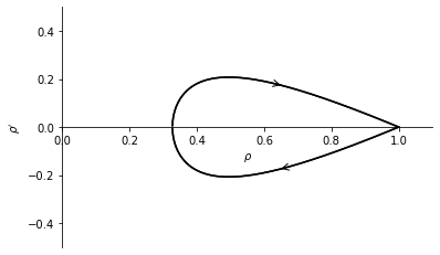
Figure 1: K=1, $\Gamma>0$, $\varepsilon=0.82$,   $G(x)=\frac{(x-1)^{2}}{2}$.

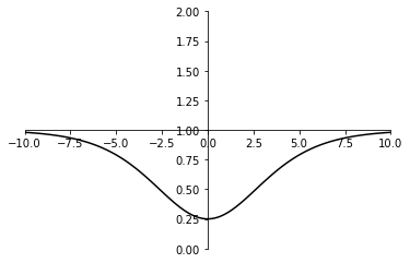
Figure 2: Graph of $\rho(x)$.

First of all we have

Lemma A.6.

For any $\varepsilon\ll 1$, $r$ is even, increasing on $]-\infty,0]$ then decreasing on $[0,+\infty[$. Moreover

$$r_{\varepsilon}(0)\underset{\varepsilon\rightarrow 0}{\longrightarrow}3,$$

and there exists a constant $C$, not depending on $\varepsilon$, such that

$$\|r^{\prime}_{\varepsilon}\|_{\infty}\leq C.$$

Proof.

The variations of r are an immediate consequence of the proposition A.4. Using (A.13) and lemma A.1 we have for $\varepsilon\ll 1$

$$3-\frac{\varepsilon}{|\gamma|}\leq r_{\varepsilon}(0)\leq 3+\frac{\varepsilon}{|\gamma|}.$$

Using (A.12) we obtain

$$\frac{\gamma^{2}}{2K(1)}K(\rho)r_{\varepsilon}^{\prime 2}=\frac{r_{\varepsilon}^{2}\gamma^{2}}{2}\bigg{(}1-r_{\varepsilon}\gamma\frac{1}{3\gamma}\bigg{)}+O(\varepsilon^{2}r_{\varepsilon}^{3}).$$

Since $K(1)\neq 0$ and   $\rho\underset{\varepsilon\rightarrow 0}{\longrightarrow}1\,\text{in}\;C^{0}(\mathbb{R})$ there exists $M$ not depending on $\varepsilon$ such that

$$\|r^{\prime}_{\varepsilon}\|_{\infty}\leq M,$$

this ends the proof. ∎

Proof of proposition A.5.

We recall that

$$-c^{2}\frac{(\rho-1)}{\rho}+\frac{c^{2}(\rho-1)^{2}}{2\rho^{2}}+g(\rho)=K(\rho)\rho^{\prime\prime}+\frac{1}{2}K^{\prime}(\rho)\rho^{\prime 2}.$$ (A.16)

After lenghty but simple computations, we find that $(r_{\varepsilon},r_{\varepsilon}^{\prime})$ is a solution of

$$X^{\prime}=f(t,X,\varepsilon),\;X(0)=\bigg{(}\begin{array}[]{c}r_{\varepsilon}(0)\\ 0\end{array}\bigg{)},$$

with

$$f :\mathbb{R}\times U\times]-\delta,\delta[\longrightarrow\mathbb{R}^{2}$$

$$f\bigg{(}t,\bigg{(}\begin{array}[]{c}r\\ r^{\prime}\end{array}\bigg{)},\varepsilon\bigg{)}=\bigg{(}\begin{array}[]{c}r^{\prime}\\ g(r,r^{\prime},\varepsilon)\end{array}\bigg{)},$$

where $U=]0,4[\times]-M-1,M+1[$,

$$g(r,r^{\prime},\varepsilon)=r-\frac{r^{2}}{2}+\varepsilon^{2}R_{1}(\varepsilon^{2}r)+\varepsilon^{2}r^{3}P_{1}(\varepsilon^{2}r)+\varepsilon^{2}R_{2}(\varepsilon^{2}r)r^{\prime 2}.$$

with $P_{1},R_{1},R_{2}\in C^{\infty}(]-1,1[)$. We recall that

$$N(x)=\frac{3}{ch^{2}(x/2)}.$$

Moreover $N$ is a solution of

$$X^{\prime}=f(t,X,0),\;X(0)=\bigg{(}\begin{array}[]{c}3\\ 0\end{array}\bigg{)}.$$

Then as $r_{\varepsilon}$ is a solution of

$$X^{\prime}=f(t,X,\varepsilon),\;X(0)=\bigg{(}\begin{array}[]{c}r_{\varepsilon}(0)\\ 0\end{array}\bigg{)},$$

with $r_{\varepsilon}(0)\rightarrow 3,$ we obtain, using the Cauchy-Lipschitz theorem with parameter, that for any compact set $[a,b]$

$$r_{\varepsilon}\underset{\varepsilon\rightarrow 0}{\longrightarrow}N,\,\text{in}\;C^{0}([a,b]),$$ (A.17)

and

$$r^{\prime}_{\varepsilon}\underset{\varepsilon\rightarrow 0}{\longrightarrow}N^{\prime},\,\text{in}\;C^{0}([a,b]).$$ (A.18)

We have using proposition A.4 and (A.13) that the functions $N,r_{\varepsilon}$ are increasing on $]-\infty,0]$, decreasing on $[0,\infty[$ and converge to 0 in $+\infty$ and $-\infty$. Thus we obtain

$$r_{\varepsilon}\underset{\varepsilon\rightarrow 0}{\longrightarrow}N,\,\text{in}\;C^{0}(\mathbb{R}).$$

which concludes the proof. ∎

The following proposition ends the proof of proposition 1.4

Proposition A.7.

We have for all $k\in\mathbb{N}$

$$\|r_{\varepsilon}^{(k)}-N^{(k)}\|_{L^{\infty}(\mathbb{R})}\underset{\varepsilon\rightarrow 0}{\longrightarrow}0.$$

Proof.

We already know the result for $k=0$, we prove it for $k=1$. We have by (A.18) uniform convergence on any compact. As $r_{\varepsilon}$ converges uniformly to $N$ and $N(x)\underset{|x|\rightarrow\infty}{\longrightarrow}0$ then $\underset{\varepsilon^{\prime}\leq\varepsilon}{sup}\,\underset{M\leq|x|}{sup}\,r_{\varepsilon^{\prime}}(x)\underset{M\rightarrow\infty}{\longrightarrow}0$. Since we have

$$\frac{\gamma^{2}}{2K(1)}K(\rho)r_{\varepsilon}^{{}^{\prime}2}=\frac{r_{\varepsilon}^{2}\gamma^{2}}{2}\bigg{(}1-r_{\varepsilon}\gamma\frac{1}{3\gamma}\bigg{)}+O(\varepsilon^{2}r_{\varepsilon}^{3}).$$ (A.19)

we obtain that $\underset{\varepsilon^{\prime}\leq\varepsilon}{sup}\,\underset{M\leq|x|}{sup}\,r_{\varepsilon^{\prime}}^{{}^{\prime}}\underset{|x|\rightarrow\infty}{\longrightarrow}0$. Moreover $N^{\prime}(x)\underset{|x|\rightarrow\infty}{\longrightarrow}0$ so we obtain

$$\forall\eta>0,\exists\varepsilon^{\prime},\exists M,\big{(}|x|>M,\varepsilon<\varepsilon^{\prime}\implies|r^{\prime}_{\varepsilon}(x)-N(x)|\leq|r^{\prime}_{\varepsilon}(x)|+|N(x)|\leq\eta\big{)},$$

combining with (A.15) we have

$$\|r_{\varepsilon}^{(1)}-N^{(1)}\|_{L^{\infty}(\mathbb{R})}\underset{\varepsilon\rightarrow 0}{\longrightarrow}0.$$ (A.20)

The result for higher order follows by use of the ODE and a simple induction argument. ∎

Remark A.8.

Using (A.5) and letting

$$u(x)=-\varepsilon^{2}\gamma v_{\varepsilon}\bigg{(}\frac{\varepsilon x}{\sqrt{K(1)}}\bigg{)},$$ (A.21)

we obtain

$$v_{\varepsilon}(x)=\frac{\sqrt{1-\varepsilon^{2}}}{1-\varepsilon^{2}\gamma r_{\varepsilon}(x)}r_{\varepsilon}(x),$$

so by the proposition A.7 we have that

$$\|r_{\varepsilon}-N\|_{L^{\infty}(\mathbb{R})}\underset{\varepsilon\rightarrow 0}{\longrightarrow}0.$$

On the other hand by using Leibniz formula one has, for all $n\in\mathbb{N}$

$$v_{\varepsilon}(x)=\sum_{k=0}^{n-1}\bigg{(}\frac{\sqrt{1-\varepsilon^{2}}}{1-\varepsilon^{2}\gamma r_{\varepsilon}(x)}\bigg{)}^{(k)}r_{\varepsilon}^{(n-k)}(x)+\bigg{(}\frac{\sqrt{1-\varepsilon^{2}}}{1-\varepsilon^{2}\gamma r_{\varepsilon}(x)}\bigg{)}r_{\varepsilon}^{(n)}(x),$$

and therefore by proposition (A.7) we have for all $n\in\mathbb{N}$

$$\|v^{(n)}_{\varepsilon}-N^{(n)}\|_{L^{\infty}(\mathbb{R})}\underset{\varepsilon\rightarrow 0}{\longrightarrow}0,$$ (A.22)

a result similar to the one obtained in dimension 2.

The case $\Gamma=0$

The proof of proposition 1.6 is similar to what was done earlier (see figure 3 for a phase portrait). let us give a heuristic argument. Substituting

$$\rho=1+\varepsilon r\bigg{(}\frac{\varepsilon x}{\sqrt{K(1)}}\bigg{)},$$

into (A.6) we find

$$\bigg{(}\frac{g^{\prime\prime\prime}(1)-12}{6}\bigg{)}r^{3}+r=r^{\prime\prime}+O(\varepsilon).$$

Then differentiating this equation we have

$$\frac{1}{2}w^{2}w^{\prime}+w^{\prime}=w^{\prime\prime\prime}.$$

where

$$w=\frac{1}{\sqrt{g^{\prime\prime\prime}(1)-12}}.$$

For a similar (and more general) result in the case of the non-linear Schrödinger equation, see [9].

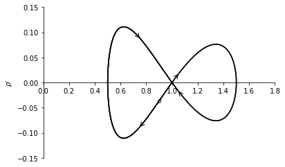
Figure 3: K=1, $\Gamma=0$, $\varepsilon$=0.5,   $G(x)=\frac{(x-1)^{2}}{2}-\frac{(x-1)^{3}}{2}$.

References

- [1] Corentin Audiard. Small energy traveling waves for the Euler–Korteweg system. Nonlinearity, 30(9):3362, 2017.
- [2] Fabrice Béthuel, Philippe Gravejat, and Jean-Claude Saut. Existence and properties of travelling waves for the Gross-Pitaevskii equation. In Stationary and time dependent Gross-Pitaevskii equations, volume 473 of Contemp. Math., pages 55–103. Amer. Math. Soc., Providence, RI, 2008.
- [3] Fabrice Béthuel, Philippe Gravejat, and Jean-Claude Saut. On the KP I transonic limit of two-dimensional Gross-Pitaevskii travelling waves. Dyn. Partial Differ. Equ., 5(3):241–280, 2008.
- [4] Fabrice Béthuel, Philippe Gravejat, and Jean-Claude Saut. Travelling waves for the Gross-Pitaevskii equation. II. Comm. Math. Phys., 285(2):567–651, 2009.
- [5] Fabrice Bethuel, Philippe Gravejat, Jean-Claude Saut, and Didier Smets. On the Korteweg–de Vries long-wave approximation of the Gross–Pitaevskii equation I. International Mathematics Research Notices, 2009(14):2700–2748, 2009.
- [6] Fabrice Bethuel, Philippe Gravejat, Jean-Claude Saut, and Didier Smets. On the Korteweg–de Vries long-wave approximation of the Gross–Pitaevskii equation II. Communications in Partial Differential Equations, 35(1):113–164, 2009.
- [7] Fabrice Béthuel, Philippe Gravejat, and Didier Smets. Asymptotic stability in the energy space for dark solitons of the Gross-Pitaevskii equation. Annales scientifiques de l’École normale supérieure, 48, 12 2012.
- [8] Rémi Carles, Raphaël Danchin, and Jean-Claude Saut. Madelung, Gross-Pitaevskii and Korteweg. Nonlinearity, 25(10):2843–2873, 2012.
- [9] D. Chiron. Travelling waves for the nonlinear Schrödinger equation with general nonlinearity in dimension one. Nonlinearity, 25(3):813–850, 2012.
- [10] David Chiron. Stability and instability for subsonic traveling waves of the nonlinear Schrödinger equation in dimension one. Anal. PDE, 6(6):1327–1420, 2013.
- [11] David Chiron. Error bounds for the (KdV)/(KP-I) and (gKdV)/(gKP-I) asymptotic regime for nonlinear Schrödinger type equations. In Annales de l’Institut Henri Poincaré C, Analyse non linéaire, volume 31, pages 1175–1230. Elsevier, 2014.
- [12] David Chiron and Sylvie Benzoni-Gavage. Long wave asymptotics for the Euler-Korteweg system. Revista Matemática Iberoamericana, 34(1):245–304, 2018.
- [13] David Chiron and M. Mariş. Rarefaction pulses for the nonlinear schrödinger equation in the transonic limit. Communications in Mathematical Physics, 326(2):329–392, 2014.
- [14] David Chiron and Mihai Mariş. Traveling waves for nonlinear Schrödinger equations with nonzero conditions at infinity. Archive for Rational Mechanics and Analysis, 226(1):143–242, 2017.
- [15] David Chiron and Eliot Pacherie. Smooth branch of rarefaction pulses for the nonlinear Schrödinger equation and the Euler-Korteweg system in 2d. In preparation.
- [16] David Chiron and Eliot Pacherie. A uniqueness result for the two vortex travelling wave in the nonlinear schrodinger equation. arXiv preprint arXiv:2109.07098, 2021.
- [17] David Chiron and Frédéric Rousset. The KdV/KP-I limit of the nonlinear Schrödinger equation. SIAM Journal on Mathematical Analysis, 42(1):64–96, 2010.
- [18] A De Bouard and JC Saut. Remarks on the stability of generalized KP solitary waves. Contemporary mathematics, 200:75–84, 1996.
- [19] Anne de Bouard and Jean-Claude Saut. Solitary waves of generalized Kadomtsev-Petviashvili equations. Ann. Inst. H. Poincaré Anal. Non Linéaire, 14(2):211–236, 1997.
- [20] Anne De Bouard and Jean-Claude Saut. Symmetries and decay of the generalized Kadomtsev–Petviashvili solitary waves. SIAM Journal on Mathematical Analysis, 28(5):1064–1085, 1997.
- [21] David Gilbarg, Neil S Trudinger, David Gilbarg, and NS Trudinger. Elliptic partial differential equations of second order, volume 224. Springer, 1977.
- [22] Philippe Gravejat. Asymptotics of the solitary waves for the generalised Kadomtsev-Petviashvili equations. Discrete and Continuous Dynamical Systems - Series A, 21(3):835–882, July 2008.
- [23] Philippe Gravejat and Didier Smets. Asymptotic stability of the black soliton for the Gross–Pitaevskii equation. Proceedings of the London Mathematical Society, 111(2):305–353, 2015.
- [24] CA Jones, SJ Putterman, and PH Roberts. Motions in a bose condensate. v. stability of solitary wave solutions of non-linear Schrödinger equations in two and three dimensions. Journal of Physics A: Mathematical and General, 19(15):2991, 1986.
- [25] CA Jones and PH Roberts. Motions in a bose condensate. IV. axisymmetric solitary waves. Journal of Physics A: Mathematical and General, 15(8):2599, 1982.
- [26] Boris Borisovich Kadomtsev and Vladimir Iosifovich Petviashvili. On the stability of solitary waves in weakly dispersing media. In Doklady Akademii Nauk, volume 192, pages 753–756. Russian Academy of Sciences, 1970.
- [27] P.-L. Lions. The concentration-compactness principle in the calculus of variations. The locally compact case. I. Ann. Inst. H. Poincaré Anal. Non Linéaire, 1(2):109–145, 1984.
- [28] Yong Liu and Juncheng Wei. Nondegeneracy, Morse index and orbital stability of the KP-I lump solution. Archive for Rational Mechanics and Analysis, 234(3):1335–1389, 2019.
- [29] P. I. Lizorkin. On multipliers of Fourier integrals in the spaces . Proc. Steklov Inst. Math., 89:269–290, 1967.