Improved binary black hole searches through better discrimination against noise transients

Abstract

The short-duration noise transients in LIGO and Virgo detectors significantly affect the search sensitivity of compact binary coalescence (CBC) signals, especially in the high mass region. In the previous work by the authors Joshi et al. (2021), a $\chi^{2}$ statistic was proposed to distinguish them from CBCs. This work is an extension where we demonstrate the improved noise-discrimination of the optimal $\chi^{2}$ statistic in real LIGO data. The tuning of the optimal $\chi^{2}$ includes accounting for the phase of the CBC signal and a well informed choice of sine-Gaussian basis vectors to discern how CBC signals and some of the most worrisome noise-transients project differently on them Choudhary et al. (2022). We take real blip glitches (a type of short-duration noise disturbance) from the second observational (O2) run of LIGO-Hanford and LIGO-Livingston detectors. The binary black hole signals were simulated using IMRPhenomPv2 waveform and injected into real LIGO data from the same run. We show that in comparison to the traditional $\chi^{2}$, the optimal $\chi^{2}$ improves the signal detection rate by around 4% in a lower-mass bin ($m_{1},m_{2}\in[20,40]M_{\odot}$) and by more than 5% in a higher-mass bin ($m_{1},m_{2}\in[60,80]M_{\odot}$), at a false alarm probability of $10^{-3}$. We find that the optimal $\chi^{2}$ also achieves significant improvement over the sine-Gaussian $\chi^{2}$. [This document has been assigned the report number LIGO-DCC-P2200288.]

I Introduction

Gravitational-wave (GW) astronomy has achieved several feats in recent years – following up on the first detection of the binary black hole merger GW150914 (Abbott et al., 2016). After the first breakthrough detection, two LIGO detectors (in Livingston and Hanford) Aasi et al. (2015) along with the Virgo detector (in Cascina) Acernese et al. (2015) have observed more than 90 compact binary coalescence (CBC) signals from various kinds of binaries involving black holes (BHs) and neutron stars (NSs) in their first three observation runs (Abbott et al., 2021). The fourth observation (O4) run is expected to start in 2023, and is expected to include KAGRA (kag, 2019). The GW community is expecting the CBC detection rate to increase significantly in O4. It is, therefore, important to find ways to effectively handle data quality and detector characterization to improve the search sensitivity so as not to miss interesting signals. Currently, high-mass CBC searches (for component mass $>60M_{\odot}$) are adversely affected by noise transients Nitz (2018); Abbott et al. (2018) and some works have developed techniques to improve the search sensitivity in that part of the CBC parameter space Kapadia et al. (2017); Nitz (2018); Mishra (2019); Joshi et al. (2021); Davis et al. (2020); Jadhav et al. (2021); Ashton et al. (2022); Choudhary et al. (2022). These works include statistical, instrumental and, recently, a few machine-learning efforts.

All studies about the sensitivity in the high-mass CBC parameter region typically mention the impact of blip glitches Cabero et al. (2019) as a major source of deterioration in the sensitivity. These glitches are a type of short-duration noise artifact found in both LIGO detectors as well as in the Virgo detector. The duration of these glitches is around 10ms. In the frequency domain they are over 100Hz wide. Recent studies on the blips in O2 run mention that they occur 2-3 times per hour in both LIGO detectors. The reason behind blips affecting the CBC search sensitivity is that their time-frequency morphology has a lot of similarity with GW signals from CBCs with high total mass, high mass-ratio or component spin and orbital angular momentum anti-aligned Nitz (2018); Joshi et al. (2021). These are essentially signals from binary black holes (BBHs).

According to recent blip studies, their source is still unknown Cabero et al. (2019). These types of glitches do not show much correlation with any of the auxiliary channels (i.e., noise source monitoring channels). Therefore, it is tricky to confirm them as non-astrophysical and remove them from short-duration signal searches. One way to veto blips from GW data is to develop a statistical test that can differentiate them from CBC signals based on their different characteristics (e.g., in spectrograms). There are $\chi^{2}$ statistics, such as the traditional-$\chi^{2}$ Allen (2005) and sine-Gaussian $\chi^{2}$ Nitz (2018), that are implemented in GW search pipelines to tackle glitches, with, especially, the latter showing some success in discriminating against blips. Still a lot of room for improvement and complementing current methods exists in this regard.

In this work, we exploit the unified $\chi^{2}$ formalism Joshi et al. (2021) to develop a new $\chi^{2}$ statistic that incorporates information about how blip glitches and BBH signals project differently on a basis of sine-Gaussian functions. Following that work, we call it the optimal sine-Gaussian $\chi^{2}$ statistic, or just the optimal sine-Gaussian $\chi^{2}$ for short. We also tune it in real data to specifically reduce the impact of blip glitches on the sensitivity of non-spinning BBH searches. Previous work in this connection – in Ref. Joshi et al. (2021) – had developed such a statistic targeting simulated sine-Gaussian transients. Spinning BBH searches will be pursued in a separate work.

This paper is organized as follows. In Sec. II, we discuss theoretical aspects of the optimal $\chi^{2}$ including a brief introduction to the general framework of the $\chi^{2}$ statistics. Sec. III describes the process of creating the optimal $\chi^{2}$. That is, how we select the basis vectors and ways to limit the number of basis vectors. Sec. IV talks about the results and performance of optimal $\chi^{2}$ in real data. Finally, in Sec. V we discuss the future applicability and prospects of this work.

II $\chi^{2}$ discriminators and their optimisation

II.1 General Framework

The general framework for $\chi^{2}$ discriminators has been described in Dhurandhar et al. (2017a). It unifies the $\chi^{2}$ discriminators and is, therefore, appropriately termed as the unified $\chi^{2}$. In this framework, a data train $x(t)$ defined over a time interval $[0,T]$ is viewed as a vector ${\bf x}$. Such data trains form a vector space ${\cal D}$. Vectors in ${\cal D}$ will be denoted in boldface, namely, ${\bf x},{\bf y}\in{\cal D}$. Since the detector strain is typically sampled at a high rate, of ${\cal O}(10^{3})\,$Hz, and the signals studied here can be as long as ${\cal O}(10^{3})\,$sec, the data vectors can have large number of components, i.e., $N\sim 10^{6}$ or larger. Hence, ${\cal D}$ is essentially the $N$-dimensional real set ${\cal R}^{N}$. When additional structure is added to ${\cal D}$, namely, that of a scalar product, then it becomes a Hilbert space.

Next consider the detector noise $n(t)$, which is a stochastic process defined over the time segment $[0,T]$. It has an ensemble mean of zero, and is stationary in the wide sense. A specific noise realisation is a vector ${\bf n}\in{\cal D}$, where ${\bf n}$ is in fact a random vector. Its one-sided power spectral density (PSD) is denoted by $S_{n}(f)$. If $\tilde{x}(f)$ and $\tilde{y}(f)$ are the Fourier representations of the vectors ${\bf x}$ and ${\bf y}$, respectively, then the scalar product of two vectors x and y in ${\cal D}$ is given by:

$$(\textbf{x},\textbf{y})=4\Re\int_{f_{\rm lower}}^{f_{\rm upper}}df\frac{\tilde{x}^{*}(f)\tilde{y}(f)}{S_{h}(f)}\,,$$ (1)

where the integration limits usually demarcate the signal band of interest, $[{f_{lower}},\,{f_{upper}}]$. We have used an integral for the scalar product because the number of components of a data vector is very large, as argued above, and the continuum limit may be taken from a sum to an integral.

The $\chi^{2}$ discriminator is a mapping from ${\cal D}$ to positive real numbers and is defined so that its value for the signal is zero and for Gaussian noise has a $\chi^{2}$ distribution with a reasonable number of degrees of freedom, $p$. Typically, the number of degrees of freedom is a few tens to a hundred. If a template ${\bf h}$ is triggered, then the $\chi^{2}$ for ${\bf h}$ is defined by choosing a finite-dimensional subspace ${\cal S}$ of dimension $p$ that is orthogonal to ${\bf h}$, i.e., for any ${\bf y}\in{\cal S}$, we must have $({\bf y},{\bf h})=0$. Then the $\chi^{2}$ for the template ${\bf h}$ is defined as just the square of the $L_{2}$ norm of the data vector ${\bf x}$ projected onto ${\cal S}$. Specifically, we perform the following operations. Take a data vector ${\bf x}\in{\cal D}$ and decompose it as:

$${\bf x}={\bf x}_{{\cal S}}+{\bf x}_{{\cal S}^{\perp}}\,,$$ (2)

where ${\cal S}^{\perp}$ is the orthogonal complement of ${\cal S}$ in ${\cal D}$. ${\bf x}_{{\cal S}}$ and ${\bf x}_{{\cal S}^{\perp}}$ are projections of ${\bf x}$ into the subspaces ${\cal S}$ and ${\cal S}^{\perp}$, respectively. We may write ${\cal D}$ as a direct sum of ${\cal S}$ and ${\cal S}^{\perp}$, that is, ${\cal D}={\cal S}\oplus{\cal S}^{\perp}$.

Then the required statistic $\chi^{2}$ is,

$$\chi^{2}({\bf x})=\|{\bf x}_{{\cal S}}\|^{2}\,.$$ (3)

The $\chi^{2}$ statistic so defined has the following properties. Given any orthonormal basis of ${\cal S}$, say ${\bf e}_{\alpha}$, with $\alpha=1,2,...,p$ and $({\bf e}_{\alpha},{\bf e}_{\beta})=\delta_{\alpha\beta}$, we obtain the following:

1. For a general data vector ${\bf x}\in{\cal D}$, we have:

   $$\chi^{2}({\bf x})=\|{\bf x}_{{\cal S}}\|^{2}=\sum_{\alpha=1}^{p}|({\bf x},{\bf e}_{\alpha})|^{2}\,.$$ (4)

2. Clearly, $\chi^{2}({\bf h})=0$ because the projection of ${\bf h}$ into the subspace ${\cal S}$ is zero, i.e., ${\bf h}_{{\cal S}}=0$.

3. Now, the noise ${\bf n}$ is taken to be stationary and Gaussian, with PSD $S_{n}(f)$ and mean zero. Therefore, the following is valid:

   $$\chi^{2}({\bf n})=\|{\bf n}_{{\cal S}}\|^{2}=\sum_{\alpha=1}^{p}|({\bf n},{\bf e}_{\alpha})|^{2}\,.$$ (5)

   Observe that the random variables $({\bf n},{\bf e}_{\alpha})$ are independent and Gaussian, with mean zero and variance unity. This is because $\langle({\bf e}_{\alpha},{\bf n})({\bf n},{\bf e}_{\beta})\rangle=({\bf e}_{\alpha},{\bf e}_{\beta})=\delta_{\alpha\beta}$, where the angular brackets denote ensemble average (see (Creighton and Anderson, 2011) for proof). Thus, $\chi^{2}({\bf n})$ possesses a $\chi^{2}$ distribution with $p$ degrees of freedom.

For convenience, one is free to choose any orthonormal basis of ${\cal S}$. In an orthonormal basis the statistic is manifestly $\chi^{2}$ since it can be written as a sum of squares of independent Gaussian random variables, with mean zero and variance unity.

In the context of CBC searches, however, we have a family of waveforms that depend on several parameters, such as masses, spins and other kinematical parameters. We denote these parameters by $\lambda^{a},~{}~{}a=1,2,...,m$. The templates corresponding to these waveforms are normalized, i.e., $\|{\bf h}(\lambda^{a})\|=1$. Then the templates trace out a manifold ${\cal P}$ – the signal manifold – which is a submanifold of ${\cal D}$. We now associate a $p$-dimensional subspace ${\cal S}$ orthogonal to the template ${\bf h}(\lambda^{a})$ at each point of ${\cal P}$ – we have a $p$-dimensional vector-space “attached” to each point of ${\cal P}$. When done in a smooth manner, this construction produces a vector bundle with a $p$-dimensional vector space attached to each point of manifold ${\cal P}$. We have, therefore, found a very general mathematical structure for the $\chi^{2}$ discriminator. Any given $\chi^{2}$ discriminator for a signal waveform ${\bf h}(\lambda^{a})$ is the square of the $L_{2}$ norm of a given data vector ${\bf x}$ projected onto the subspace ${\cal S}$ at ${\bf h}(\lambda^{a})$.

It can be easily shown that the traditional $\chi^{2}$ falls under the class of unified $\chi^{2}$. This is done by exhibiting the subspaces ${\cal S}$ or by exhibiting the basis vector field for ${\cal S}$ over ${\cal P}$; the conditions mentioned above must be satisfied by ${\cal S}$. In (Dhurandhar et al., 2017b) such a basis field has been exhibited explicitly.

II.2 Optimising the $\chi^{2}$ discriminator

The $\chi^{2}$ discriminator must produce as large a value as possible for a glitch in the data. In our framework we achieve this, on average, given the collection of glitches. The optimisation is therefore carried out for a family of glitches, say, ${\cal G}$. Here we will model the glitches as sine-Gaussians and select a family of such glitches based on the ranges of the parameters describing the sine-Gaussians. The subspace ${\cal S}$ then must be chosen in such a way as to have maximum projection on an average. Also one must keep in mind that ${\cal S}$ must be orthogonal to the trigger template. These two criteria essentially guide us to obtain the subspaces ${\cal S}$. The third criterion is that its dimension should be kept small in order to keep the computational cost at a reasonable level.

More specifically for a given trigger template ${\bf h}$, we perform the following steps:

1. Sample the parameter space ${\cal G}$ of the glitches (sine-Gaussians) sufficiently densely so that the sample is representative. We call the subspace of ${\cal D}$ spanned by these sampled vectors as ${\mathcal{V}}_{{\cal G}}$. This is done efficiently and conveniently with the help of a metric, as will be described in Sec. III.1.

2. Since ${\cal S}$ should be orthogonal to ${\bf h}$, we remove the component parallel to ${\bf h}$ from each of the sample vectors spanning ${\mathcal{V}}_{{\cal G}}$. Thus if ${\bf v}\in{\mathcal{V}}_{{\cal G}}$, then we define ${\bf v}_{\perp}={\bf v}-({\bf v},{\bf h}){\bf h}$. These vectors ${\bf v}_{\perp}$ by construction are orthogonal to ${\bf h}$. The space spanned by these clipped vectors ${\bf v}_{\perp}$ is called ${\mathcal{V}}_{\perp}$.

3. Next we apply Singular Value Decomposition (SVD) to the row vectors of ${\mathcal{V}}_{\perp}$ to obtain the best possible approximation of lower dimension say $p$. We will put a cut-off on the singular values so that projection obtained is as large as desired, say, $90\%$. The singular vectors corresponding to the singular values obtained by applying the cut-off generate the subspace ${\cal S}$.

For further details of procedure we refer to (Dhurandhar et al., 2017b). In the next section, Sec. III.1, we describe how one can define a metric on ${\cal G}$ to obtain the sample vectors that span ${\mathcal{V}}_{{\cal G}}$.

III Constructing the optimal $\chi^{2}$ discriminator

III.1 Selection of vectors that span ${\mathcal{V}}_{{\cal G}}$

In order to form an optimal $\chi^{2}$, it is important that we select appropriate vectors in ${\mathcal{V}}_{{\cal G}}$ to project the GW data on. In order to improve the sensitivity of CBC searches, we specifically target the blip glitches in this work, which are a major source of reduction in CBC search sensitivity. A recent work Joshi et al. (2021) demonstrates how transient bursts represented by sine-Gaussian waveform Chatterji can be vetoed with the help of an optimal $\chi^{2}$ from the GW data. Since the blip glitches are also known to have a time-domain morphology similar to the sine-Gaussian waveforms, we use these waveforms to form the vectors in ${\mathcal{V}}_{{\cal G}}$ for constructing an optimal-$\chi^{2}$. To allow for an arbitrary phase, we use a complex-valued sine-Gaussian waveform. This is an improvement over our earlier work Joshi et al. (2021), especially relevant in dealing with the general scenario. In the time domain the sine-Gaussian waveform can be defined as,

$$\psi(t;t_{0},f_{0},Q)= A\exp{\bigg{(}-\frac{4\pi^{2}f_{0}^{2}}{Q^{2}}(t-t_{0})^{2}\bigg{)}}$$ (6)

$$\exp{[-i2\pi f_{0}(t-t_{0})]}\,.$$

In the frequency domain, it is

$$\tilde{\psi}(f;t_{0},f_{0},Q)= \tilde{A}\exp{\bigg{(}-\frac{Q^{2}}{2\pi f_{0}^{2}}(f-f_{0})^{2}\bigg{)}}$$ (7)

$$\exp{[-i2\pi t_{0}(f-f_{0})]}\,,$$

where $t_{0}$ is central time, $f_{0}$ is central frequency, $Q$ is the quality factor, and the amplitudes are $A=\bigg{(}\frac{8\pi f_{0}^{2}}{Q^{2}}\bigg{)}^{\frac{1}{4}}$ and $\tilde{A}=\bigg{(}\frac{Q^{2}}{2\pi f_{0}^{2}}\bigg{)}^{\frac{1}{4}}$.

To calculate the metric in the ($t_{0},f_{0},Q$) space we begin by considering two neighboring sine-Gaussian waveforms in that space, namely, $\psi_{1}(f;t_{0},f_{0},Q)$ and $\psi_{2}(f;t_{0}+dt_{0},f_{0}+df_{0},Q+dQ)$. A metric may then be introduced on this space as a map from the differences in the parameters of these waveforms to the fractional change in their match:

$$ds^{2}= \bigg{(}\frac{4\pi^{2}f_{0}^{2}}{Q^{2}}\bigg{)}dt_{0}^{2}+\bigg{(}\frac{2+Q^{2}}{4f_{0}^{2}}\bigg{)}df_{0}^{2}+\bigg{(}\frac{1}{2Q^{2}}\bigg{)}dQ^{2}$$ (8)

$$-\bigg{(}\frac{1}{2f_{0}Q}\bigg{)}df_{0}dQ.$$

We do not consider the noise power spectral density (PSD) to calculate the metric since it has negligible effect on the arrangement of the vectors in ${\mathcal{V}}_{{\cal G}}$ Chatterji . The above metric (in Eq. (8)) can be reduced to its diagonal form using the transformations,

$$\omega_{o}=2\pi f_{0}$$ (9)

and

$$\nu=\frac{\omega_{o}}{Q}\,.$$ (10)

In the new coordinates, $(t_{0},\omega_{0},Q)$, the metric takes the form

$$ds^{2}=\nu^{2}dt_{0}^{2}+\frac{1}{4\nu^{2}}d\omega_{0}^{2}+\frac{1}{2\nu^{2}}d\nu^{2}.$$ (11)

In comparison to the metric in Ref. Joshi et al. (2021), this metric has no $\omega_{0}$ term multiplying $dt_{0}^{2}$. This results from our accounting for the aforementioned arbitrary phase of the sine-Gaussian waveform in this work.

As mentioned in Ref. Bose et al. (2016), a CBC template is triggered with a time lag $t_{d}$ after the occurrence of a glitch, i.e., after $t_{0}$. The time $t_{d}$ is given by Bose et al. (2016),

$$t_{d}\simeq\tau_{0}\bigg{(}1-\frac{16}{3Q^{2}}\bigg{(}\zeta+\frac{2}{3}\bigg{)}\bigg{)}\,,$$ (12)

where the second term inside the parentheses determines the magnitude of the “correction” beyond the chirp time $\tau_{0}$, which is given by

$$\tau_{0}=\frac{5}{256\pi f_{0}}(\pi\mathcal{M}f_{0})^{-5/3},$$ (13)

and $\zeta$ is negative of the logarithmic derivative of the noise PSD ($S_{h}(f)$) evaluated at $f_{0}$.

The metric in Eq. (11) can be reduced to a more simplified form with the help of transformations

$$z=(\omega_{0}\mathcal{M})^{-5/3}\quad{\rm and}\quad y=\ln(\nu/\rm{rad/sec})\,,$$ (14)

such that

$$ds^{2}=\Bigg{[}\frac{2^{-14/3}}{Q^{2}}+\frac{9Q^{2}}{100z^{2}}\Bigg{]}dz^{2}+\frac{1}{2}dy^{2}.$$ (15)

By examining Eq. (12), one may reckon that for $Q\sim 2$ the $t_{d}$ would be significantly affected. This is in fact so but it turns out that it makes little difference to the metric. This can be seen as follows. In Eq. (12) the correction term is inversely proportional to $Q^{2}$; therefore, for high $Q$, say, with $Q\gtrsim 5$, it is negligible. Also, at high central frequencies, i.e., $f_{0}\gtrsim 500$ Hz, the factor $(\zeta+2/3)$ is small for the aLIGO design PSD. Thus, in either case one has $t_{d}\approx\tau_{0}$. The remaining case is one where $f_{0}\sim 100$ Hz and $Q\sim 2$. Now the term arising from $t_{d}$ is the second term multiplying $dz^{2}$ in the metric expression Eq. (15). It turns out that this term is small compared to the first one in the same metric expression – about 14% at this frequency. Hence, even if the $t_{d}$ is changed significantly, it makes a small difference to the metric. To summarize, in most of the parameter space we consider, the metric given in Eq. (15) applies and our sampling based on this metric valid to a good approximation.

From a broader perspective, the main idea is to sample the parameter space of glitches adequately, so that they are not misidentified. Thus, any inadequacy resulting from inaccuracies of the metric can be easily remedied by more densely sampling the parameter space. This can be achieved by just increasing the match between neighbouring points. We have explored this possibility and find that it does not lead to dissimilar results.

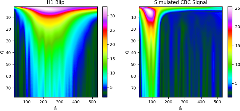
Figure 1: The sine-Gaussian projection map of an H1 blip from the O2 run with SNR = 16 (left) and a simulated BBH event injected in real noise from H1 O2 run with the same SNR (right). Here the SNRs for the blip and the CBC signal are obtained via identical matched-filtering operations. The colorbar represents relative values of the projections (Choudhary et al., 2022).

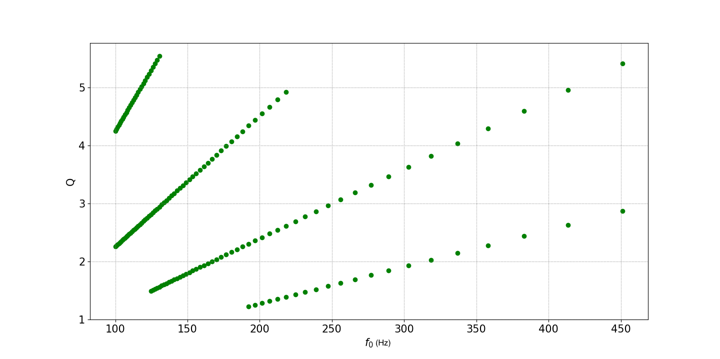
Figure 2: Sampled points in the $z-y$ space (top) for a triggered template with component masses (70,70) $M_{\odot}$, and a chirp mass of 60.9 $M_{\odot}$. The rectangular region $f_{0}\in[100,500]\,$Hz and $Q\in[2,8]$, in the $f_{0}-Q$ space (bottom), transforms to a trapezium in the $z-y$ space. Neighboring points have a minimum match of 80% and are essentially uniformly placed in the $z-y$ plane. There are a total of 58 sampled points in this plot. This number can vary with the chirp mass of the triggered template.

To choose the appropriate vectors in ${\mathcal{V}}_{{\cal G}}$ for the optimal-$\chi^{2}$, we take help from the sine-Gaussian projection maps introduced in Ref. Choudhary et al. (2022). The SGP maps are a projection of GW data onto the sine-Gaussian parameter space. We experimented with several real blips and simulated CBC signals to model their projections on the sine-Gaussian parameter space. As seen in Fig. 1, blips and CBC signals show projection in distinct regions of the sine-Gaussian parameter space. Blips project strongly in the frequency region above 100 Hz, whereas for the CBC signals with component masses above 10 $M_{\odot}$ the projection lies mostly below 100 Hz. Along the $Q$ coordinate, the CBC signals show more elongated features than the blips. This difference in the projections of blips and CBCs on sine-Gaussians paves the way for selecting appropriate vectors in ${\mathcal{V}}_{{\cal G}}$ to formulate an optimal-$\chi^{2}$ following the unified $\chi^{2}$ formalism Dhurandhar et al. (2017a). We choose parameter ranges such that the blips have a high projection on these vectors that lead to higher values of the $\chi^{2}$ statistic for blips than CBC signals. In our case, we find $f_{0}\in[100,500]$ Hz and $Q\in[2,8]$.

To construct the ${\mathcal{V}}_{{\cal G}}$ vectors in the chosen region of the sine-Gaussian parameter space we first use Eq. (15) to sample points in the $z$-$y$ space. The coefficients of $dz^{2}$ depend on $Q$, $f_{0}$ and the chirpmass $\mathcal{M}$ through the parameter $z$. To get a flat metric in $z$-$y$ space, we fix $Q=8$ and $f_{0}=500$ Hz. The choice of $Q$ and $f_{0}$ is made after observing that it provides sufficiently dense sampled points such that the mismatch between two neighbouring vectors is not more than 0.20. After sampling points in the $z$-$y$ space, we transform them back to the $Q$-$f_{0}$ space. The top panel of Fig. 2 shows points sampled in the $z$-$y$ space, while the bottom panel shows the same points after transforming to the $Q$-$f_{0}$ space. Sine-Gaussian waveforms are chosen corresponding to each of these sampled points. The number of total points can vary depending on the chirp mass $\mathcal{M}$ of the triggered template. This can lead to a large number of vectors. To reduce that number, note that most of them are not linearly independent. We, therefore, use singular value decomposition (SVD) (discussed below in Sec. III.2) to obtain the (much smaller number of) basis vectors from that sample. The resultant SVD vectors are then used to project the GW data upon them using Eq. (1). As it turns out, we require just about three vectors – on which the data show maximum projection – to compute the optimal-$\chi^{2}$, which is then defined as,

$$\chi_{\rm opt}^{2}=\sum_{\alpha=1}^{3}|(\textbf{x},\textbf{g}_{\alpha})|^{2}\,,$$ (16)

where x is the data vector and $\textbf{g}_{\alpha}$ are the three aforementioned basis vectors.

III.2 Reducing the number of degrees of freedom of the $\chi^{2}$

The selected vectors (sine-Gaussians) as described in Section III.1 usually turn out to be quite large in number. After time-shifting the sine-Gaussians and clipping their components parallel to the template, they span the subspace ${\mathcal{V}}_{\perp}$ (see Section II.2). We could in principle use ${\mathcal{V}}_{\perp}$ on which to project the data vector and compute the $\chi^{2}$ statistic. But the dimension of ${\mathcal{V}}_{\perp}$ is usually large and in practice it would involve too much computational effort and slow down the search pipeline – the $\chi^{2}$ would involve too many degrees of freedom, namely, the dimension of ${\mathcal{V}}_{\perp}$. Therefore, we look for the best $p$-dimensional approximation to ${\mathcal{V}}_{\perp}$, where $p$ is reasonably small. The SVD algorithm allows us to achieve just this – this is the essence of the Eckart-Young-Mirsky theorem (Eckart and Young, 1936).

However, the SVD cannot be applied directly to the selected vectors in ${\mathcal{V}}_{{\cal G}}$. The input matrix, say, $M$ needs to be first prepared. We briefly describe the procedure here since the full details can be found in (Joshi et al., 2021). The following are the salient steps needed:

• The sine-Gaussians have central time $t_{0}=0$ and they need to be appropriately time-shifted with respect to the time of occurrence of the trigger. We will always take the trigger to occur at $t=0$, and so the glitch must have occurred at time $-t_{d}$. Accordingly the sine-Gaussians have to be shifted by the time $-t_{d}$. Since we write the input matrix in the Fourier domain, this is achieved by multiplying each row vector by the phase factor $e^{2\pi ift_{d}}$.

• The selected vectors need to be clipped by subtracting out from each sine-Gaussian its component parallel to the template. The clipped and time-shifted sine-Gaussians span the subspace ${\mathcal{V}}_{\perp}$ of ${\cal D}$. The desired subspace ${\cal S}$ is a subspace of ${\mathcal{V}}_{\perp}$.

• The usual SVD algorithm “sees” the Euclidean scalar product. However, here we have a weighted scalar product – inversely weighted by the PSD $S_{h}(f)$. So in order the apply the usual SVD algorithm we need to whiten each row vector. This is achieved by dividing each Fourier component of the row vector by $\sqrt{S_{h}(f)}$.

• The input matrix is now ready to be fed into the SVD algorithm.

This is however not the end of the story. We have to also modify the output - which are the right singular vectors. We need to unwhiten these vectors by multiplying by the factor $\sqrt{S_{h}(f)}$. The unwhitened singular vectors are orthonormal in the weighted scalar product.

The SVD algorithm also yields singular values $\sigma_{i},~{}i=1,2,...,r$. The Frobenius norm of the input matrix is just $\parallel M\parallel_{F}=\sum_{i=1}^{r}\sigma_{i}^{2}$. The number of degrees of freedom $p$ are chosen so that:

$$\sum_{i=1}^{p}\sigma_{i}^{2}~{}\gtrsim~{}(1-\delta)~{}\parallel M\parallel_{F}\,,~{}~{}~{}~{}~{}~{}~{}~{}~{}~{}~{}~{}p~{}\leq~{}r,$$ (17)

where $\delta$ may be chosen to be, say, $0.1$ or 10 %. The subspace ${\cal S}$ is generated by the first $p$ right singular vectors and so has dimension $p$. This also means that we have a projection of about $90\%$, on the subspace ${\cal S}$. ${\cal S}$ is the best $p$ dimensional approximation to ${\mathcal{V}}_{\perp}$ – it is essentially a $p$-dimensional least-square fit to ${\mathcal{V}}_{\perp}$ (see (Joshi et al., 2021) for more discussion). We have also succeeded in reducing the number of degrees of freedom of the $\chi^{2}$ to $p$. Typically, for the ranges of parameters $f_{0},~{}Q,~{}{\mathcal{M}}$, etc., considered here, the number of selected vectors in ${\mathcal{V}}_{{\cal G}}$ is about a few hundred while $p<10$. Thus, $p$ is much smaller than the number of selected vectors in ${\mathcal{V}}_{{\cal G}}$.

IV Results

In this study we tuned the optimal-$\chi^{2}$ specifically for the blip glitches. In order to test the effectiveness of the optimal-$\chi^{2}$ in differentiating the blips from non-spinning BBH signals, we chose real blips from the LIGO O2 run, as identified by the Gravity Spy tool Zevin et al. (2017); Bahaadini et al. (2018); Coughlin et al. (2019); Soni et al. (2021); Glanzer et al. (2022). Blips were selected from both Hanford and Livingston detectors when they had a confidence level of 0.6 on a scale of 0 to 1, as rated by Gravity Spy. A total of 4000 strain data segments, each of length 16 sec and containing a blip with a matched-filtering signal-to-noise ratio (SNR) between 4 and 30, were chosen. The BBH data sample is prepared by simulating the BBH signals using the family of IMRPhenomPv2 waveforms  Hannam et al. (2014). The simulated BBH signals also span the same SNR range, namely, 4 to 30, uniformly. We divide the signals into two classes based on their component masses: one class consists of signals with component masses $m_{1},m_{2}\in[20,40]M_{\odot}$ and the other consists of $m_{1},m_{2}\in[60,80]M_{\odot}$. The purpose of the classification was to compare the performance of the optimal-$\chi^{2}$ in the two ranges of masses and use it to understand which part of the BBH parameter space is adversely affected by the blips thereby making the search sensitivity worse for the adversely affected class. For the studies in this section, we needed 3 (complex) basis vectors in Eq. (16) for the construction of the optimal-$\chi^{2}$, which amounts to 6 degrees of freedom for that statistic.

Figure 3: The figure on the left shows different types of $\chi^{2}$ vs SNR scatter plots. The corresponding ROC plots for blips vs BBH signals are shown on the right. Here we use 4000 real O2 H1 blips and 4000 simulated CBC signals with component masses uniformly distributed in range $[20,40]M_{\odot}$. To calculate the SNR in this case we have used a CBC template bank with total mass $M_{\rm total}\in[30,90]M_{\odot}$ and mass ratio $q\in[1,10]$.

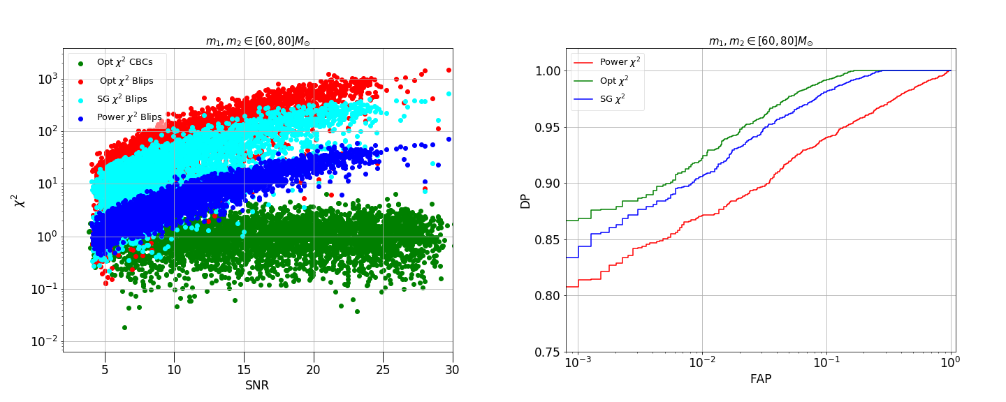
Figure 4: This figure is similar to Fig. 3 but for a different range of masses. Similar to that figure, here we plot 4000 real O2 H1 blips and 4000 simulated CBC signals with component masses uniformly distributed in the range [60,80] $M_{\odot}$. To calculate the SNR in this case we have used a CBC template bank with total mass $M_{\rm total}\in[100,180]M_{\odot}$ and mass ratio $q\in[1,10]$. As seen in the right figure, the optimal $\chi^{2}$ performs better than the other two alternatives in this experiment in real data.

To calculate the SNR for both the blips and and BBHs signals, we use different CBC template banks for the two classes. For lower masses $m_{1},m_{2}\in[20,40]$, we use a template bank with total mass $M_{\rm total}\in[30,90]M_{\odot}$ and $q\in[1,10]$. For higher masses, $m_{1},m_{2}\in[60,80]$, we use a template bank with the range of total masses $M_{\rm total}\in[100,180]M_{\odot}$ and $q\in[1,10]$. The BBH signals so prepared are injected into 16 sec long data segments from O2 that are not known to have any astrophysical signals in them. These data segments are multiplied with the Tukey window in order to make smooth transition to zero at the edges, which takes care of any possible spectral leakage during the analysis.

We use the receiver-operating characteristic (ROC) curves to assess the performance of the optimal $\chi^{2}$ and compare it with that of the traditional $\chi^{2}$ and sine-Gaussian $\chi^{2}$ statistics. First, the optimal, traditional and sine-Gaussian $\chi^{2}$s are calculated for the chosen sample of BBHs and blips, in addition to their respective SNRs, as shown in Fig. 3 and Fig. 4. We then use the ranking statistic defined in Ref. Nitz et al. (2021); Usman et al. (2016) to rank the triggers in case of traditional $\chi^{2}$. On the other hand, for sine-Gaussian and optimal $\chi^{2}$ we use the new ranking statistic defined in Ref. Nitz (2018). The choice of ranking statistic for traditional and sine-Gaussian $\chi^{2}$ is the usual one. The decision to use the new ranking statistics in case of optimal $\chi^{2}$ was made after finding how both ranking statistics affect the performance of the optimal $\chi^{2}$. As we can see from the ROC curves in Fig. 3 and Fig. 4 (right panel), the optimal $\chi^{2}$ performs better than the traditional and sine-Gaussian $\chi^{2}$ at all false alarm probabilities in both classes. With optimal $\chi^{2}$, we are able to achieve an improvement in sensitivity of around 4% over the traditional $\chi^{2}$ at false alarm probability of $10^{-2}$ for lower masses $m_{1},m_{2}\in[20,40]$. For higher masses $m_{1},m_{2}\in[60,80]M_{\odot}$, we see that the optimal $\chi^{2}$ shows improvement in sensitivity of more than 5% at false alarm probability of $10^{-2}$. The optimal $\chi^{2}$ performs better than the traditional $\chi^{2}$ irrespective of the masses, and moreover there is significant improvement in the sensitivity over the sine-Gaussian $\chi^{2}$.

The optimal $\chi^{2}$ performs better since it accounts for the differences and similarities between blips and BBH waveforms quantitatively by utilizing the metric in the sine-Gaussian space Joshi et al. (2021). The performance improvement is superior for higher mass BBHs because those signals occupy a lower part of the frequency band compared to the blips. The improvement over the sine-Gaussian $\chi^{2}$ can be understood in terms of the choice of $Q$ and $f_{0}$ range while sampling the sine-Gaussian waveforms to construct the ${\mathcal{V}}_{{\cal G}}$ vectors and then subtracting the triggered templates from them. This work makes a few advances compared to the previous implementation of the optimal $\chi^{2}$ Joshi et al. (2021). For instance, here we utilized the complex form of the sine-Gaussian waveforms to account for the phase of the signal. Moreover, the sine-Gaussian projection maps Choudhary et al. (2022) helped us in identifying appropriate regions in the sine-Gaussian parameter space to choose the ${\mathcal{V}}_{{\cal G}}$ vectors from for the construction of the optimal $\chi^{2}$ statistic. These advances also helped in bringing about appreciable improvement in CBC search sensitivity over traditional and sine-Gaussian $\chi^{2}$.

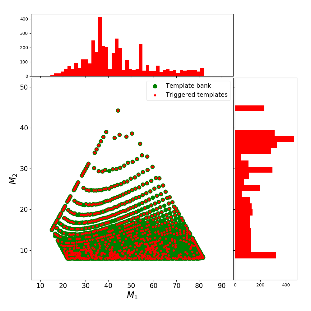
Figure 5: The component masses of all templates employed are shown in green. In contrast, the red ones (which are their subset) show the templates that are triggered by any of the (real) blips from a sample of 4000 – taken from Livingston and Hanford detectors’ O2 run. Corresponding to each mass axis, there is a histogram showing the number of templates triggered at each component mass value.

It must be emphasized that just like for the traditional $\chi^{2}$, the computation of the optimal $\chi^{2}$ uses the parameter values of the triggered template. Therefore, the choice of template-bank boundaries while doing the matched-filtering operation can play an important role in its effectiveness. As we can see in the Fig. 5, blips can trigger a wide variety of templates, and a narrow template bank choice can adversely affect the performance of the optimal $\chi^{2}$.

V Discussion

Owing to their time-frequency morphological similarity with high-mass BBH signals, the short-duration noise transients affect the search sensitivity of those signals adversely. In this study, we showed how the optimal $\chi^{2}$ can be constructed in real LIGO data so as to reduce that impact. The previous version of optimal $\chi^{2}$ introduced in Ref. Joshi et al. (2021) is further tuned here to veto the blip glitches. A few advances have been made here compared to past works on the optimal $\chi^{2}$ discriminator that have helped us in achieving a modest improvement over the existing $\chi^{2}$ tests. The first one was accounting for the phase of the signal in the construction of the basis vectors – by using complex sine-Gaussian waveforms. The second contributor was the use of projection maps Choudhary et al. (2022), which guide us in locating the region in sine-Gaussian parameter space from which the initial sine-Gaussians should be chosen for constructing the basis vectors used in computing the optimal $\chi^{2}$.

The computational cost per trigger of the optimal $\chi^{2}$ is higher than that of the traditional $\chi^{2}$ and the sine-Gaussian $\chi^{2}$. A major fraction of this cost arises from the construction of orthonormal basis vectors described in Sec. III.2. This makes the implementation of the optimal $\chi^{2}$ in an online search less efficient computationally. A straightforward way to reduce this inefficiency is to construct the orthonormal basis vectors beforehand for a set of template masses. In case of a high-mass template-bank, this advance preparation can be done for all the templates, as their number is relatively small. In case of low-mass template-banks, a more sparsely-populated fraction of templates can be selected for pre-computation of the orthonormal basis vectors. The optimal $\chi^{2}$ is then computed using the basis vectors of the nearest template.

As noted before, there have been some attempts to veto blip glitches from the data with the help of a $\chi^{2}$ like statistic (Nitz, 2018) and machine learning networks (McIsaac and Harry, 2022; Choudhary et al., 2022) – claiming varying degrees of improvement in the BBH search sensitivity. Some of these works exploit certain insights provided by the unified $\chi^{2}$ formalism (Dhurandhar et al., 2017a) but so far none of them fully leverages the power afforded by it. The work reported in this paper attempted to bridge that gap – for non-spinning BBH signals. It will be important to extend this work to explore possible mitigation of the blips’ effect on spinning CBC searches. Since prograde spinning systems can push the innermost stable circular orbit to frequencies higher than their non-spinning counterparts, the former signals are expected to have a greater overlap with the blip glitches, which makes their discrimination less effective. However, since BBH signals project better on higher $Q$ sine-Gaussians than blips, involving the optimal $\chi^{2}$ in spinning searches may help in improving their sensitivities. Spinning BBH signals can be pursued in a future study.

VI Acknowledgment

We would like to thank Sudhagar Suyamprakasam and Tanmaya Mishra for discussions related to LIGO data. We also thank Bhooshan Gadre for reviewing the manuscript and sharing some useful comments. SVD acknowledges the support of the Senior Scientist Platinum Jubilee Fellowship from the National Academy of Sciences, India (NASI). The data analysis and simulations for this work were carried out at the IUCAA computing facility Sarathi. This research has made use of data, software, and/or web tools obtained from the Gravitational Wave Open Science Center (Abbott and et. al., 2019; gwo, ), a service of LIGO Laboratory, the LIGO Scientific Collaboration, and the Virgo Collaboration. Some of that material and LIGO are funded by the National Science Foundation. Virgo is funded by the French Centre National de Recherche Scientifique (CNRS), the Italian Istituto Nazionale della Fisica Nucleare (INFN), and the Dutch Nikhef, with contributions by Polish and Hungarian institutes. We also use some of the modules from the PyCBC an open source software package (Nitz et al., 2021).

References

- Joshi et al. (2021) P. Joshi, R. Dhurkunde, S. Dhurandhar, and S. Bose, Physical Review D 103 (2021), 10.1103/physrevd.103.044035.
- Choudhary et al. (2022) S. Choudhary, A. More, S. Suyamprakasam, and S. Bose, “Sigma-net: Deep learning network to distinguish binary black hole signals from short-duration noise transients,” (2022).
- Abbott et al. (2016) B. P. Abbott et al. (LIGO Scientific Collaboration and Virgo Collaboration), Phys. Rev. Lett. 116, 061102 (2016).
- Aasi et al. (2015) J. Aasi, B. P. Abbott, R. Abbott, T. Abbott, M. R. Abernathy, K. Ackley, C. Adams, T. Adams, P. Addesso, and et al., Classical and Quantum Gravity 32, 074001 (2015).
- Acernese et al. (2015) F. Acernese, M. Agathos, K. Agatsuma, D. Aisa, N. Allemandou, A. Allocca, J. Amarni, P. Astone, G. Balestri, G. Ballardin, et al., Classical and Quantum Gravity 32, 024001 (2015), arXiv:1408.3978 [gr-qc] .
- Abbott et al. (2021) R. Abbott, T. Abbott, S. Abraham, F. Acernese, K. Ackley, A. Adams, C. Adams, R. Adhikari, V. Adya, C. Affeldt, and et al., “Gwtc-3: Compact binary coalescences observed by ligo and virgo during the second part of the third observing run,” (2021), arXiv:2111.03606 [gr-qc] .
- kag (2019) Nature Astronomy 3, 35–40 (2019).
- Nitz (2018) A. H. Nitz, Class. Quant. Grav. 35, 035016 (2018), arXiv:1709.08974 [gr-qc] .
- Abbott et al. (2018) B. P. Abbott, R. Abbott, T. D. Abbott, M. R. Abernathy, F. Acernese, K. Ackley, C. Adams, T. Adams, P. Addesso, R. X. Adhikari, and et al., Classical and Quantum Gravity 35, 065010 (2018).
- Kapadia et al. (2017) S. J. Kapadia, T. Dent, and T. Dal Canton, Phys. Rev. D 96, 104015 (2017), arXiv:1709.02421 [astro-ph.IM] .
- Mishra (2019) T. Mishra, Developing methods to distinguish between CBC signals and glitches in LIGO, Master’s thesis, NISER, Bhubaneswar (2019).
- Davis et al. (2020) D. Davis, L. V. White, and P. R. Saulson, Classical and Quantum Gravity 37, 145001 (2020), arXiv:2002.09429 [gr-qc] .
- Jadhav et al. (2021) S. Jadhav, N. Mukund, B. Gadre, S. Mitra, and S. Abraham, Phys. Rev. D 104, 064051 (2021).
- Ashton et al. (2022) G. Ashton, S. Thiele, Y. Lecoeuche, J. McIver, and L. K. Nuttall, Class. Quant. Grav. 39, 175004 (2022), arXiv:2110.02689 [gr-qc] .
- Cabero et al. (2019) M. Cabero et al., Class. Quant. Grav. 36, 155010 (2019), arXiv:1901.05093 [physics.ins-det] .
- Allen (2005) B. Allen, Phys. Rev. D71, 062001 (2005), arXiv:gr-qc/0405045 [gr-qc] .
- Dhurandhar et al. (2017a) S. Dhurandhar, A. Gupta, B. Gadre, and S. Bose, Physical Review D 96 (2017a), 10.1103/physrevd.96.103018.
- Creighton and Anderson (2011) J. D. E. Creighton and W. G. Anderson, Gravitational-wave physics and astronomy: An introduction to theory, experiment and data analysis (John Wiley & Sons, Ltd, 2011).
- Dhurandhar et al. (2017b) S. Dhurandhar, A. Gupta, B. Gadre, and S. Bose, Phys. Rev. D96, 103018 (2017b), arXiv:1708.03605 [gr-qc] .
- (20) S. K. Chatterji, “The search for gravitational wave bursts in data from the second ligo science run,” http://hdl.handle.net/1721.1/34388.
- Bose et al. (2016) S. Bose, S. Dhurandhar, A. Gupta, and A. Lundgren, Physical Review D 94 (2016), 10.1103/physrevd.94.122004.
- Eckart and Young (1936) C. Eckart and G. Young, Psychometrika 1, 211 (1936).
- Zevin et al. (2017) M. Zevin, S. Coughlin, S. Bahaadini, E. Besler, N. Rohani, S. Allen, M. Cabero, K. Crowston, A. K. Katsaggelos, S. L. Larson, T. K. Lee, C. Lintott, T. B. Littenberg, A. Lundgren, C. Østerlund, J. R. Smith, L. Trouille, and V. Kalogera, Classical and Quantum Gravity 34, 064003 (2017).
- Bahaadini et al. (2018) S. Bahaadini, V. Noroozi, N. Rohani, S. Coughlin, M. Zevin, J. Smith, V. Kalogera, and A. Katsaggelos, Information Sciences 444, 172 (2018).
- Coughlin et al. (2019) S. Coughlin, S. Bahaadini, N. Rohani, M. Zevin, O. Patane, M. Harandi, C. Jackson, V. Noroozi, S. Allen, J. Areeda, and et al., Physical Review D 99 (2019), 10.1103/physrevd.99.082002.
- Soni et al. (2021) S. Soni, C. P. L. Berry, S. B. Coughlin, M. Harandi, C. B. Jackson, K. Crowston, C. Østerlund, O. Patane, A. K. Katsaggelos, L. Trouille, and et al., Classical and Quantum Gravity 38, 195016 (2021).
- Glanzer et al. (2022) J. Glanzer, S. Banagiri, S. B. Coughlin, S. Soni, M. Zevin, C. P. L. Berry, O. Patane, S. Bahaadini, N. Rohani, K. Crowston, and C. Østerlund, “Data quality up to the third observing run of advanced ligo: Gravity spy glitch classifications,” (2022), arXiv:2208.12849 [gr-qc] .
- Hannam et al. (2014) M. Hannam, P. Schmidt, A. Bohé, L. Haegel, S. Husa, F. Ohme, G. Pratten, and M. Pürrer, Phys. Rev. Lett. 113, 151101 (2014).
- Nitz et al. (2021) A. Nitz, I. Harry, D. Brown, C. M. Biwer, J. Willis, T. D. Canton, C. Capano, T. Dent, L. Pekowsky, A. R. Williamson, G. S. C. Davies, S. De, M. Cabero, B. Machenschalk, P. Kumar, D. Macleod, S. Reyes, dfinstad, F. Pannarale, T. Massinger, S. Kumar, M. Tápai, L. Singer, S. Khan, S. Fairhurst, A. Nielsen, S. Singh, K. Chandra, shasvath, and B. U. V. Gadre, “gwastro/pycbc:,” (2021).
- Usman et al. (2016) S. A. Usman, A. H. Nitz, I. W. Harry, C. M. Biwer, D. A. Brown, M. Cabero, C. D. Capano, T. D. Canton, T. Dent, S. Fairhurst, and et al., Classical and Quantum Gravity 33, 215004 (2016).
- McIsaac and Harry (2022) C. McIsaac and I. Harry, Phys. Rev. D 105, 104056 (2022).
- Abbott and et. al. (2019) R. Abbott and et. al. (LIGO Scientific Collaboration and Virgo Collaborration), (2019), arXiv:1912.11716 [gr-qc] .
- (33) “Gravitational Wave Open Science Center,” https://www.gw-openscience.org/, accessed: 2022-04-20.