Fine-grained Image Editing by Pixel-wise Guidance Using Diffusion Models

Abstract

Our goal is to develop fine-grained real-image editing methods suitable for real-world applications. In this paper, we first summarize four requirements for these methods and propose a novel diffusion-based image editing framework with pixel-wise guidance that satisfies these requirements. Specifically, we train pixel-classifiers with a few annotated data and then infer the segmentation map of a target image. Users then manipulate the map to instruct how the image will be edited. We utilize a pre-trained diffusion model to generate edited images aligned with the user’s intention with pixel-wise guidance. The effective combination of proposed guidance and other techniques enables highly controllable editing with preserving the outside of the edited area, which results in meeting our requirements. The experimental results demonstrate that our proposal outperforms the GAN-based method for editing quality and speed. Code is available at https://github.com/sony/pixel-guided-diffusion.git 

1 Introduction

Recently, generative models have been widely utilized in many image-editing methods  [15, 55] thanks to their potential to generate high-quality visual content. Several techniques have already been applied to real-world applications by digital artists [7] and have contributed to expanding their creativity. To reflect the user’s intention to the details in edited images more effectively, we focus on fine-grained real image editing.

We refer to fine-grained image editing as an editing process with pixel-level control that does not generate new content but makes small and localized changes to the appearance of existing content in the image, such as manipulating facial parts and animal pose shown in Fig.1. Considering the real-world application of this editing process, it requires four properties:

P.1

visual content in the editing area should be created aligned with the user’s intent down to the pixel,

P.2

the content outside the edited area should be precisely preserved, and

P.3

it can be built in a label-efficient manner to apply it to a new category easily, and

P.4

fast editing should be possible.

Jointly meeting these requirements leads to higher controllability and better user experience.

In the literature, GANs (Generative Adversarial Networks)  [18] have been intensely adopted. GAN-based methods can precisely reflect fine-grained instruction by users, such as manipulated semantic segmentation map  [29, 36, 59, 30] , skethes [12] into edited images. Notably, EditGAN [30] is specifically designed to learn such editing in a label-efficient manner. Although these methods successfully provide high-quality visual content in the edited area, it is essentially difficult to strictly preserve other contents in the target image (i.e. P.2), as shown at the bottom of Fig.1 because it requires solving a challenging problem which is to find the latent features corresponding to the edited image while satisfying such constraints. In summary, many GAN-based methods satisfy P.1 and P.4, and EditGAN further satisfies P.3, but it is inherently difficult for these methods to satisfy P.2, which would result in a serious barrier to their use in real-world applications.

To address the above-mentioned issue while meeting four properties, we propose a novel diffusion-based editing method that enables fine-grained editing by user-provided manipulated segmentation map as shown in Fig. 1. Compared to the prior works, we use diffusion models instead of GANs. It is effective to satisfy P.2, but makes it challenging to satisfy P.3 and P.4 in general. Therefore, we extend DatasetDDPM [8], which is a label-efficient semantic segmentation model, to every time step and use it to guide the generation process of reverse diffusion process based on pixel-wise segmentation loss (for P.1 and P.3). Additionally, we adopt accelerated generation  [16] to this pixel-level guidance to achieve comparable editing speed to the GAN-based method (for P.4). Experimental results validate the advantage of our method both quantitatively and qualitatively.

In summary, our contributions are three-fold:

• We reveal that fine-grained real image editing for real-world applications can be achieved with an effective combination of pixel-wise guidance and other techniques.

• We reveal that the optimal setting of both start denoising step $t_{0}$ and guidance scale $s$ depends on the size of the edited area. This is helpful in determining the parameter setting for unseen data on applications.

• Our pixel-wise guidance is more computationally efficient than the conventional guidance using full-size segmentation models. It contributes to fast editing.

2 Related Works

2.1 Diffusion models

Denoising Diffusion Probabilistic Model (DDPM) [20, 47, 34, 16] is a generative model that aims to generate data by reversing a diffusion process. The forward diffusion process is defined as a Markov chain process with time, where a small amount of Gaussian noise is added to samples in $T$ steps, resulting in $x_{T}$ following an isotropic Gaussian distribution. A single step in this process can be represented by the following equation: $q(x_{t}|x_{t-1})\coloneqq\mathcal{N}(\sqrt{1-\beta_{t}}x_{t-1},\beta_{t}I)$, where $\beta_{t}$ is the hyperparameter that defines the process. If $\beta_{t}$ is sufficiently small, the step of the reverse diffusion process $q(x_{t-1}|x_{t})$ can also be parameterized by a Gaussian transition as follows: $p_{\theta}(x_{t-1}|x_{t})\coloneqq\mathcal{N}(\mu_{\theta}(x_{t},t),\Sigma_{\theta}(x_{t},t)),$ the mean $\mu_{\theta}$ and covariance $\Sigma_{\theta}$ is estimated by $x_{t}$ which is an input of the noise estimator $\epsilon_{\theta}(x_{t},t)$, where $\theta$ is parameterized by the U-net encoder and the decoder. The model is trained to obtain $\mu$ via noise estimation for $x_{t}$, while $\Sigma$ is assumed to be fixed in DDPM. Consequently, we can represent a single step in the reverse process as follows:

$$x_{t-1}=\frac{1}{\sqrt{1-\beta_{t}}}\Biggl{(}x_{t}-\frac{\beta_{t}}{\sqrt{1-\bar{\alpha}_{t}}}\epsilon_{\theta}(x_{t},t)\Biggr{)}+\sigma_{t}\epsilon,$$ (1)

where $\alpha_{t}:=1-\beta_{t},\bar{\alpha}_{t}:=\prod_{s=1}^{t}\alpha_{s},\epsilon\sim\mathcal{N}(0,I)$. Given an initial $x_{T}$, we generate a sample by repeating the above step from $t=T$ to $t=0$.

Data generation through DDPM is stochastic, as shown in Eq. 1. Therefore, given a fixed $x_{T}$, we can obtain various $x_{0}$ through this process. Conversely, [48] extends DDPM to obtain a deterministic generation process by utilizing a non-Markovian forward process. A single step of the reverse process in DDIM is described as follows:

$$x_{t-1}= \sqrt{\bar{\alpha}_{t-1}}f_{\theta}(x_{t},t)+\sqrt{1-\bar{\alpha}_{t-1}}\epsilon_{\theta}(x_{t},t),$$ (2)

$$f_{\theta}(x_{t},t)\coloneqq\frac{x_{t}-\sqrt{1-\bar{\alpha}_{t}}\epsilon_{\theta}(x_{t},t)}{\sqrt{\bar{\alpha}_{t}}}.$$ (3)

In this setting, given target data $x_{0}$, we can obtain the latent variable $x_{T}$ to generate $x_{0}$ through DDIM by repeating the following computation:

$$x_{t+1}=\sqrt{\bar{\alpha}_{t+1}}f_{\theta}(x_{t},t)+\sqrt{1-\bar{\alpha}_{t+1}}\epsilon_{\theta}(x_{t},t).$$ (4)

Using Eq. 4 and Eq. 2, DDIM achieves accurate reconstruction (inversion).

Classifier Guidance

Classifier guidance  [16] is a technique that enables pre-trained unconditional diffusion models to generate images corresponding to a specified class label. It requires a pre-trained classifier to specify the desired class and uses it to guide the generation process of the diffusion models. Specifically, classifier $p_{\phi}(y|x_{t},t)$ is first trained with noisy images $x_{t}$ that correspond to each time step $t$ in the diffusion process. Then, in the generation process, the mean of the distribution of $x_{t}$ is shifted at each time step by adding the gradients of the classifier with respect to the data, as follows:

$$p_{\theta}(x_{t-1}|x_{t})=\mathcal{N}(\mu_{\theta}(x_{t},t)+s\Sigma\nabla_{x_{t}}\mathrm{log}\ p_{\phi}(y|x_{t},t),\Sigma),$$ (5)

where $s$ is the guidance scale parameter.

Semantic Segmentation with Diffusion Models

The proposed method builds on DatasetDDPM [8], which is a label-efficient semantic segmentation model that uses pixel-level representations of the noise estimator $\epsilon_{\theta}$. The authors called the model trained on synthetic images is called DatasetDDPM. Therefore, this paper calls the model trained on real images as DatasetDDPM-R. DatasetDDPM-R estimates a segmentation label on each pixel via a three-layer multi-layer perceptron (MLP), which is referred to as a pixel-classifier. The input of this classifier is the UNet’s intermediate activations which are upsampled and concatenated. Furthermore, DatasetDDPM [8] outperforms DatasetGAN [58] in segmentation estimation performance because real images can be used for training.

2.2 Image Editing Methods

GAN-based methods

Generative Adversarial Network (GAN)  [18]-based editing methods are divided into various categories. There are those, for example, that find a meaningful and disentangled direction in latent spaces in an unsupervised manner [56, 45, 46, 10, 9, 39, 53] and those that use text [27, 38, 17, 54]. These methods are helpful for concept-level editings, such as style transfer and attribute transformation, but are unsuitable for localized and fine-grained editing.

To achieve fine-grained editing, some approaches use segmentation maps and sketches for user-provided inputs [29, 36, 59, 12]. These methods achieve precise editing of details corresponding to the manipulation of user-provided inputs, but their drawback is that a large amount of annotated data is required for conditional training. EditGAN [30] solve this problem by building on DatasetGAN [58], which consists of a simple three-layer MLP classifiers with the middle features of StyleGAN [22, 23] as inputs. This classifier predicts the segmentation label on each pixel, and as a result, EditGAN can achieve high-precision editing in a label-efficient manner.

However, when editing real images, the GAN-based methods listed above first need to search for appropriate latent variables that can reconstruct the images via a generator. Although, there are many inversion techniques [1, 2, 3, 42, 51, 59, 4] for searching such latent variables, these GAN-based methods, including EditGAN suffer from the incomplete reconstruction of features that are scarce in training data. That could be a major drawback limiting their real-world editing applications.

Diffusion-based methods

Diffusion models  [20, 47, 34, 16] and score-based generative models [49, 50] are suitable for real image editing because it has outperformed image synthesis quality  [16] against existing generative models [11, 26, 52, 32, 41] and can be accurately reconstructed, as described in the Sec.2.1. Some works have been conducted in a global manner [24, 40], which can be applied to style and attribute transformations, but is unsuitable for localized, fine-grained editing.

For fine-grained editing, some works can be divided into two categories. One line of research is training the conditional diffusion models [35, 43]. We can edit images locally using an inpainting technique  [43] and text-prompts [35] by training diffusion models using such conditions as inputs. However, these methods incur high training costs because they are required to train the diffusion models.

On the other hand, unconditional model based methods [13, 31, 6, 5], it can use the pre-trained diffusion models, achieve editing with low training cost. ILVR [13] is an image translation method in which the low-frequency component is used for conditioning the sampling process, and it achieves scribble-based editing. In SDEdit [31], user-provided strokes on images are first noised in the latent spaces by a stochastic SDE process. The edited images are then generated by denoising via the reverse SDE process. These methods achieve user-provided localized editing, but they cannot easily edit fine-grained features. In particular, for SDEdit, there is no guarantee that the edited content will be preserved through the generation process because no conditions related to the edit are given in a simple stochastic reverse SDE process. Blended-diffusion  [5, 6] is a technique for localized editing that corresponds to user-provided text prompts. But it is unsuitable for fine-grained editing, such as ”Growing hair a little longer,” via the text descriptions.

Therefore, we propose the localized and fine-grained image editing method in a label-efficient manner.

3 Fine-grained Edit with Pixel-wise Guidance

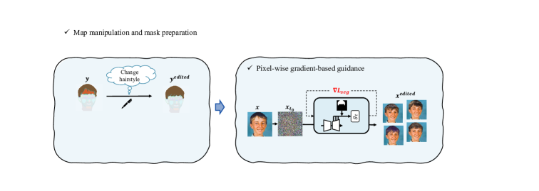
Figure 2: Overall workflow of the proposed method. (a) For preparation, we train pixel classifiers of DatasetDDPM-R [8], which is an MLP-based segmentation model, and save parameters. (b) After training, we estimate the segmentation map using intermediate representations across multiple steps (50,150,250 steps concatenate). (c) We then manipulate the segmentation map into desired one. (d) In the iterative reverse denoising process, we guide the sampling process with the gradient of a pixel classifier $G_{t}$.

3.1 Overview

The overall flow of the proposed method for image editing is shown in Fig. 2. First, we train pixel classifier  [8] $G_{multi}$ and $G_{t}$, which is used to estimate a segmentation map for editing and pixel-wise guidance, respectively. Then, we denote the set of $G_{t}$ by $G$. For map manipulation, we generate the original segmentation map $y$ of a target real image $x$ by applying the pixel classifier $G_{multi}$ to $x$ and then manipulate it to the desired map $y^{edited}$. Furthermore, we guide the reverse diffusion process with the gradient of a pixel classifier $G_{t}$ with respect to the data at each time step $t$. Finally, we obtain edited images $x^{edited}$. Detailed descriptions are given in the following sections.

3.2 Editing Framework

Training Pixel Classifiers

We use the pixel classifiers $G$ of DatasetDDPM-R for gradient-based guidance. This is because we can use them to (a) build segmentation models in a label-efficient manner and, (b) reduce the computational cost because noise and label estimation can be computed simultaneously on the same forward path; furthermore, we can (c) apply it to any pre-trained non-conditional diffusion model.

Similar to the classifier guidance mentioned in Sec.2.1, the intuitive approach is to extend the classifier to accept time step $t$ as input, but this is difficult with tiny MLP-based classifier, so in this study, $G_{t}$ is trained at each time steps $t$. When training a pixel-classifier $G_{t}$, we use image-label pairs, which require human annotation. For each time step $t$, we use noise samples $x_{t}$, obtained directly from data $x_{0}$, as training data.

$$x_{t}=\sqrt{\bar{\alpha_{t}}}x_{0}+\sqrt{1-\bar{\alpha_{t}}}\epsilon,\quad\epsilon\sim\mathcal{N}(0,I).$$ (6)

Here, the label annotated on $x_{0}$ is associated with $x_{t}$ and used for training as image-label pairs. Then, we save the parameters of $G_{t}$. As we mentioned on Sec.2.1, $G_{t}$ estimates the segmentation label on each pixel, and the intermediate activations are extracted from the U-Net decoder.

For estimating the original map $y$ as described in Fig. 2 (b), we train another pixel-classifier $G_{multi}$ with the representations across multiple time steps, which are extracted from $t$={50, 150, 250} and concatenated, following the original paper [8].

Map manipulation and mask preparation

After estimating the original segmentation map $y$ using $G_{multi}$ , the user can manipulate map $y$ and then obtain the target map $y^{edited}$ as described in Fig. 2 (c). Simultaneously, we set the binary ROI mask $m$ by picking up all edit-related pixels from the original map $y$ and manipulated map $y^{edited}$ as follows [30].

$$m_{ij}=\begin{cases}1&\mathrm{if}\ y_{ij}\in Q_{edit}\ \mathrm{or}\ y^{edited}_{ij}\in Q_{edit},\\ 0&\mathrm{otherwise.}\end{cases}$$ (7)

$m\in\mathbb{R}^{H\times W}$ is a binary mask, defined by all pixels $p$ whose segmentation labels $y_{p}$ are included in the edit-related class list $Q_{edit}$, which is to be preliminarily specified manually. To seamlessly blend the edited region with the outside of the region, this $m$ is dilated for three pixels as a buffer.

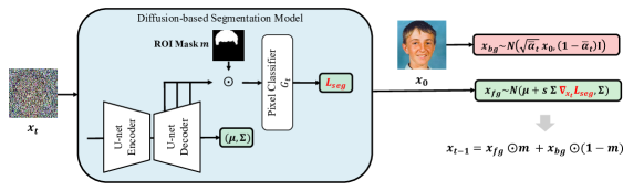
Figure 3: Overview of pixel-wise segmentation guidance at a time-step $t$. The input of the segmentation model is the masked region’s ($m$) pixel features. We obtain mean and variance on the normal denoising process and gradient of segmentation loss on the segmentation model’s output. Then we can obtain guided foreground images that are in the ROI by pixel-wise guidance.

Pixel-wise gradient-based guidance

To generate images corresponding to the edited map $y^{edited}$, we guide the reverse diffusion process using this map. First, we obtain the starting noise sample $x_{t_{0}}$ that was determined by $x_{0}$ using Eq.4. Then, we guide the sampling process at each time step $t$ for $t=t_{0},...1$, and an overview of the pixel-wise guidance at each time step is shown in Fig. 3.

Along with noise estimation, we extracted the intermediate activations $z\in\mathbb{R}^{H\times W\times d}$, which are appropriately upsampled and concatenated. Following  [8], we set $d$=2816, which is the dimension of intermediate representations at a single time step, in this paper. For this guide, we use only pixels inside the binary ROI mask $m$ as input to the pixel classifier $G_{t}$ and then obtain the gradient of the cross-entropy loss $L_{ce}$ which was averaged by the number of pixels $N=\sum_{ij}\mathbb{I}(m_{ij}=1)$ as follows:

$$L_{seg}(z,y^{edited})=\frac{1}{N}\sum_{i=1}^{H}\sum_{j=1}^{W}m_{ij}L_{ce}\Bigl{(}G_{t}(z_{ij}),y_{ij}^{edited}\Bigr{)}.$$ (8)

After obtaining the gradient, we guide the sampling process according to Eq.5 as follows.

$$x_{\mathrm{fg}}\sim\mathcal{N}(\mu+s\Sigma\nabla_{x_{t}}L_{seg},\Sigma),$$ (9)

where $\mu=\mu_{\theta}(x_{t},t),\Sigma=\Sigma_{\theta}(x_{t},t)$. This foreground term is related to the edit region. Following [6], we obtain background term by simply adding noise to the original image $x_{0}$ to preserve the outside of the edited region and combine these two terms to construct $x_{t-1}$ as follows:

$$x_{t-1,\mathrm{bg}}\sim\mathcal{N}(\sqrt{\bar{\alpha}_{t}}x_{0},(1-\bar{\alpha}_{t})I),$$ (10)

$$x_{t-1}=x_{t-1,\mathrm{fg}}\odot m+x_{t-1,\mathrm{bg}}\odot(1-m),$$ (11)

where $\odot$ denotes the element-wise multiplication. This guidance procedure is summarized in Algorithm. 1.

Algorithm 1 Pixel-wise gradient-based guidance

0:  original image $x$, target map $y^{edited}$, ROI mask $m$, guidance scale $s$, start denoising step $t_{0}$, pixel classifiers $G$

0:  edited image $x^{edited}$

  $N\leftarrow\sum_{ij}\mathbb{I}(m_{ij}=1)$

  $x_{0}\leftarrow x$

  for $t=0$ to $t_{0}-1$ do

     $x_{t+1}\leftarrow\sqrt{\bar{\alpha}_{t+1}}f_{\theta}(x_{t},t)+\sqrt{1-\bar{\alpha}_{t+1}}\epsilon_{\theta}(x_{t},t)$

  end for

  for $t=t_{0}$ down to $1$ do

     $\mu,\Sigma\leftarrow\mu_{\theta}(x_{t},t),\Sigma_{\theta}(x_{t},t)$

     $L_{seg}\leftarrow\frac{1}{N}\sum_{i=1}^{H}\sum_{j=1}^{W}m_{ij}L_{ce}\Bigl{(}G_{t}(z_{ij}),y_{ij}^{edited}\Bigr{)}$

     $x_{t-1,\mathrm{fg}}\sim\mathcal{N}(\mu+s\Sigma\nabla_{x_{t}}L_{seg},\Sigma)$

     $x_{t-1,\mathrm{bg}}\sim\mathcal{N}(\sqrt{\bar{\alpha}_{t}}x_{0},(1-\bar{\alpha_{t}})I)$

     $x_{t-1}\leftarrow x_{t-1,\mathrm{fg}}\odot m+x_{t-1,\mathrm{bg}}\odot(1-m)$

  end for

  return  $x^{edited}$

4 Experiments

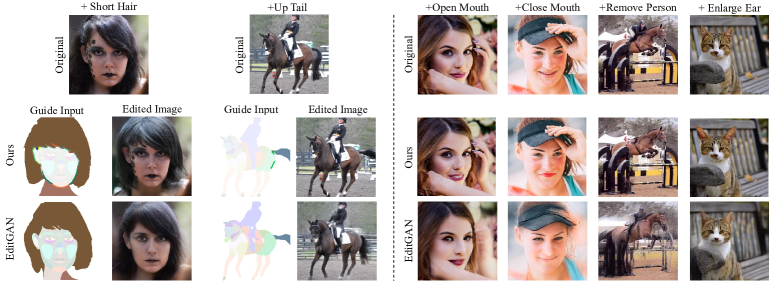
Figure 4: Qualitative comparions with EditGAN. These results were obtained by editing the segmentation map to follow the written text(e.g. + Open Mouth). The left two samples show the edited map, which is included to clarify the specified manipulation. These results confirm that our method achieves the desired editing performance while preserving the details of the original images, whereas EditGAN fails to reconstruct some features, which are less observed in training data, such as facial painting, a person, and hands in original images.

In this section, we demonstrate the quantitative and qualitative comparisons with some baseline methods. We aim to achieve fine-grained editing in a label-efficient manner. Therefore, we chose EditGAN [30] and SDEdit [31] as the baseline methods, which can work with few ore zero annotated training data, respectively.

4.1 Experimental Setting

Datasets

In all editing experiments, we used $256^{2}$ images. We used FFHQ-256 [22], LSUN-cat [57] and LSUN-horse [57] for the EditGAN experiments, and CelebA-HQ [21] for the SDEdit experiments. For training of pixel-classifiers, we used the same number of annotated images and classes as DatasetDDPM [8], but in the CelebA-HQ experiments, we used the backbone diffusion models and pixel-classifiers trained on FFHQ-256, because it is composed of more classes than the default CelebA-HQ number of classes of 19, and it provides higher editability. We used the annotated dataset as published in the DatasetDDPM official repository  

Implementation

To train the pixel classifiers, we trained only a single pixel classifier $G_{t}$ at each time step $t$ as a guidance model. For guidance, we set hyper parameters {$t_{0}$, $s$} = {$500$,$100$} for the manipulation of small parts and {$750$,$40$} for large parts of FFHQ-256, CelebA-HQ and LSUN-Cat. And we show the editing performance using full-step guidance. For accelerated guidance, we use respaced generation [16] such that the total step is 50 steps. The size of these parts was divided by a threshold of 5000 in terms of the number of pixels in the binary ROI mask $m$. On LSUN-Horse, we set $\{t_{0},s\}$=$\{800,25\}$. Additionally, in all experiments, we set the batch-size to four. With these settings, the overall edit is finished in 15 $\sim$ 30 seconds on a single NVIDIA A100 GPU when we applied respaced editing.

In the EditGAN experiments, we used optimization-based editing in [30] because this approach, while increasing the editing time, offers the most accurate editing performance among the proposed approaches in EditGAN. Then, we performed 100 steps of optimization using Adam [25] to optimize the latent codes.

In the SDEdit experiments, we used VP-SDE [31], pre-trained on the CelebA-HQ dataset, for localized image manipulation on CelebA-HQ. For all manipulations, we used stroke-based editing with $t_{0}=0.5$, $N=500$, and $K=1$. In all manipulations, we create guide inputs as described in Fig.11 of  [31] with PaintApp. The other implementation details are described in the appendix.

Evaluation Metrics

Our goal is to achieve fine-grained editing while preserving the content outside of the edited region and fast editing comparable to the GAN-based method. Therefore, we evaluated the reconstruction performance, the accuracy of manipulation, and the quality of the edited whole images and runtime for quantitative evaluation. We used MAE and PSNR to evaluate the reconstruction performance. These metrics are calculated for pixels outside the editing region, defined by the binary ROI mask $m$ in Sec.3.2. For manipulation performance, we evaluated the prediction accuracy against the target map $y_{edited}$ by predicting the map corresponding to the edited images $x_{edited}$ with DatasetGAN and DatasetDDPM-R. Subsequently, Inception Score (IS) [44] and Fréchet Inception Distance (FID) [19] were used to ensure semantic consistency between the reconstructed and manipulated regions. For the FID, we measured the distance between two distributions of the original images before editing and edited images. We measured runtime under the same batch size set to 1.

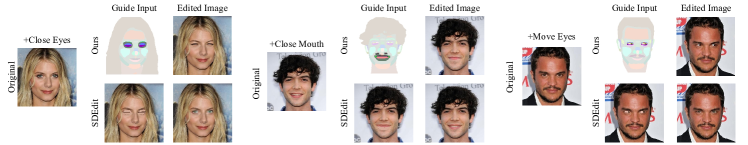
Figure 5: Qualitative comparison of our proposed method and SDEdit. We adopted stroke-based editing in SDEdit and experimented using VP-SDE ($t_{0}$=0.5, $N$=500). The guide input, which was edited with strokes using image editing software (e.g. Paint app, Photoshop), were used for editing. As a result, we confirmed that SDEdit failed to edit details (e.g. move eyes) that our porposed method edited.

Table 1: Quantitative evaluation with EditGAN on FFHQ-256 for randomly selected 50 samples. In this table, we investigated the several results of our method depending on the guidance step and the strategy of selecting edited images within batch size. In (b), we also report the standard deviation. The results revealed that the proposed method outperforms EditGAN on all evaluation metrics.

Method		$m$=0			whole image			$m$=1		Runtime [sec]
		MAE (×$10^{3}$) ↓	PSNR ↑		FID ↓	IS ↑		Accuracy ↑
EditGAN		74.85	67.24		79.67	3.765		81.38		16.28
(a) Ours (fullstep / quantitative)		14.25	81.44		15.81	4.377		83.02		146.48
(b) Ours (fullstep / random)		13.93 $\pm$ 1.742	81.59 $\pm$ 0.02958		14.62 $\pm$ 1.005	4.459 $\pm$ 0.03649		81.95 $\pm$ 00.1742		146.48
(c) Ours (50 step / quantitative)		17.26	81.48		18.61	4.933		80.74		15.30

4.2 Evaluation and Comparison

Quantitative Comparison

In this experiment, we randomly selected 50 images on FFHQ-256 and then predicted the original segmentation map with segmentation models (i.e. DatasetGAN and DatasetDDPM-R), and applied one of the following manipulations: {”close mouth,” ”open mouth,” ”move eye,” ”close eye,” ”edit eyebrow,” ”change hairstyle”} on the segmentation map. Our method can generate diverse outcomes owing to the probabilistic process of diffusion models, then we present our results in several settings in Table. 1, such as (a) selecting a quantitatively superior sample within the batch size using full-step guidance, (b) random selection using full-step guidance and (c) selecting a quantitatively superior sample within the batch size using respaced generation. As a result, we confirmed that the proposed method outperformed EditGAN in all metrics and it is not sensitive to the selection strategies. Additionally, we achieved comparable editing speed to EditGAN [30] using respaced generation. This accelerated generation is useful for real-world applications.

Qualitative Comparison

First, we show the a comparison with EditGAN [30] in Fig.1 and Fig.4. In these figures, we show the results obtained by the operation of the segmentation map as described in the text (e.g., Open Mouth). From these figures, we confirmed that EditGAN failed to reconstruct some features, which are less observed in training data, such as the pacifier, face paintings, and the hands around the face, because of an inaccurate inversion performance. This could be a significant challenge for applications that edit photos captured in the real world. In addition, for some operations, such as editing a ponytail and short hair in Fig.4, EditGAN fails to achieve the desired editing on a default set of parameters. In contrast, our method achieved the desired fine-grained editing naturally while preserving other features that were not reconstructed in EditGAN.

We then show a comparison with SDEdit [31] in Fig.5. For SDEdit, we use stroke-based edited images (Guide Input) as input to the SDE. The manipulations are shown in Fig.5 and our aim is to compare the fine-grained editability. The results reveal that SDEdit fails to edit such precise features of images, which can be achieved with our method.

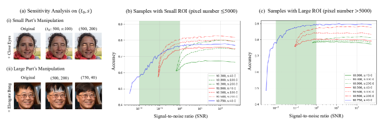
Figure 6: Analysis of the effect of the hyper-parameters, start denoising step $t_{0}$ and guidance scale $s$, on the prediction accuracy. This figure shows the relationship between signal-to-noise ratio (SNR) and accuracy on 50 experimental samples which were divided into two groups according to the size of editing region. This accuracy is averaged on each grouped samples and calculated against the estimated map on each step. When the SNR magnitude is between $10^{-2}$ and $10^{0}$, the perceptually recognizable content are generated [14].

4.3 Further Applications

The proposed methods can be utilized for some applications such as interpolation and inpainting. For interpolation, we use real images and their manipulated results (or both manipulated results) as the two inputs. We then interpolate the latent variables $x_{t_{0}}$ of these inputs, which are obtained using Eq.4, to 50 samples, and reconstruct their images with Eq.2. In Fig. 7, we show the representative samples and interpolate variables at time step $t_{0}$ = 500. These results demonstrate that we can obtain meaningful interpolated samples on the latent space of the diffusion model if these changes are minute. However, if there is a large difference between inputs, as shown in the examples of hairstyle change, the interpolated samples become slightly blurred. This is because there is no guarantee that the manipulated samples will follow a linear relationship with the original images. However, these editing vectors might be useful for controlling the intensity of editing, as in EditGAN. For the inpainting, one of the results is presented in Fig.4 (”remove person”). It requires a large start step of $t$=800, but we can confirm that the region with the person has been replaced naturally with the background.

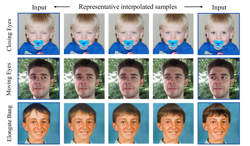
Figure 7: Results of interpolation between edited and original images. The results demonstrated the capability of meaningful interpolation on the latent space of pre-trained diffusion models.

4.4 Detailed Analysis

Sensitivity Analysis

In this section, we analyze the sensitivity of hyper-parameters, the start denoising step $t_{0}$ and the guidance scale $s$, on the editing performance. We demonstrate the relationship between signal-to-noise ratio (SNR) at each time step and prediction accuracy within the binary ROI mask $m$ in Fig.6. We experimented at $t_{0}$={300,500,750} and $s$={40,100,200}, respectively. The larger $s$ than $s$=40 on $t_{0}$=750 has made artifacts because the large value of $s$ could guide the samples to the outside the learned distribution, so it is not shown in the figure. In this experiment, we divided 50 experimental samples, which were the same samples in Sec.4.2, into two groups: those with more than 5000 pixels within the binary ROI mask $m$ (Fig. 6) and those with less than 5000 (Fig. 6). The accuracy between the target map $y_{edited}$ and the output of $G_{t}$ at each step, and averaged over the samples in the group.

First, we shall discuss $t_{0}$. From Fig.6 (b) and (c), we confirmed that the manipulation of large regions requires a large $t_{0}$, while that of a small region can be achieved with a small $t_{0}$. This is because a large content of images are created in the early step of the reverse diffusion process [14, 8, 28], which is visualized on a green background [14]. A small content was created after that. In Fig.6 (a), the results of the manipulation of a large region demonstrated that no matter how large the guidance scale $s$ is (such as $s$=200), it is difficult to change global features with a small step $t_{0}$=500, as this results in an unnatural edit.

Next, we analyze the effect of the guidance scale $s$. The results of manipulating a small region in Fig.6 (a) also reveal that a large scale $s$ generates images that are too aligned to a specified class and fail to generate realistic outcomes. Therefore, we considered that $s$=100 was suitable on when we set $t_{0}$=500. We, therefore, set ($t_{0}$,$s$) = ($500$,$100$) for the manipulation of small regions and ($750$,$40$) for the manipulation of large regions on the face and cat datasets. However, for LSUN horse manipulation, where an object is placed in the background and an object is generated on the background, we set a large value of $t_{0}$=800 and $s$ was set to 25 because a large value of $s$ is likely to shift the mean of $x_{t}$ outside the learned distribution on large $t_{0}$.

Limitations

There are a few cases that a large denoising step is necessary even if the manipulation is small when we manipulate the eyebrow or mouth with orthodontics. In such cases, the user is required to manually adjust the step after observing the outcomes. Additionally, as the proposed edit is based on class labels, the manipulation is restricted within the learned class label, and there are cases in which the original content color has been changed through editing. (e.g., eye color, hair color).

5 Conclusion

In this paper, we summarized the requirements of real-world fine-grained image editing frameworks and proposed a novel image editing method with pixel-wise guidance using diffusion models. The effective combination of our label-efficient guidance and other techniques enabled highly controllable editing with preserving the outside of the edited area at a fast speed, meeting our requirements. While the automatic setting of hyper-parameters and color controls remain as our future work.

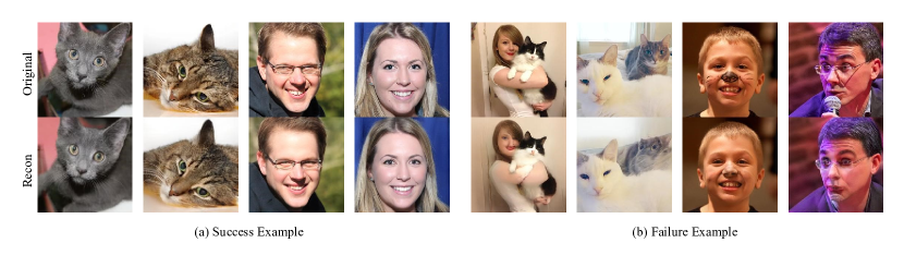
Figure 9: Results of the reconstruction performance in EditGAN. The latent codes corresponding to these original images are obtained by optimization after initialized by trained image encoder  [30]. These results demonstrate that the contents, which is less observed in the training data (e.g., ”microrophone”, ”another cat”), were inaccurately reconstracted by EditGAN.

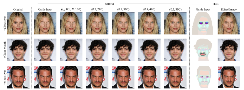
Figure 10: Comparison of stroke-based image editing performance with $t_{0}$ in SDEdit. We show the edited images with different values of $t_{0}$ in SDEdit. For SDEdit, we use VP-SDE  [31] and set $K$ = 1. These results reveal that SDEdit has a strict trade-off between the faithfulness and realism. It is difficult for the users to adjust the appropriate $t_{0}$ manually.

Appendix A Implementation Details

A.1 Pixel Classifiers

The proposed method uses ADM  [16] for backbone diffusion models and we used pre-trained ADM model provided in  [8]. We respectively trained a single neural network for $g_{t}$ and $g_{multi}$, whereas the original DatasetDDPM [8] used an ensemble of ten individual networks. In this work, we used the intermediate representations extracted from the decoder block $B$ = 5,6,7,8,12 at each time step; therefore, the total dimensions of the pixel-wise features were 2816. We used the same training conditions and model architecture as in their paper [8]. We trained them for 4 epochs, using the Adam [25] optimizer with learning rate of 0.001. The batch size was set to 64. These settings are used for all datasets.

A.2 EditGAN

EditGAN [30] consists of three components, which are a generator of StyleGAN2, an image encoder for inversion, and DatasetGAN [58] for estimation of segmentation maps. As for the generator, we used the pretrained model, which is publicly available at the official repository . Only for FFHQ-256, we used the pretrained model available at another repository, because this is not provided at the official one.

Regarding the image encoder, we used the same model architecture as in the literature  [30]. We trained the encoder using the Adam optimizer with learning rate of $3\times 10^{-5}$. In their implementations, they train only on generated samples from GAN for first 20,000 iterations as warm up and then train jointly real and generated images on LSUN-Cat dataset. We applied this warm up training not only to LSUN-Cat but also to LSUN-Horse. In FFHQ, we trained without warm up. For inference, we refine the latent code, which is initialized by this encoder, via 500-steps optimization as described in  [30].

As for pixel classifiers of DatasetGAN, we used the same annotated data for training. As in their setup [30], we trained ten independent segmentation models, each of which is a three-layer MLP classifier  [58], using the Adam optimizer with learning rate of 0.001. Other training implementation details were same as the original configurations [30].

Appendix B Additional Results

B.1 Reconstruction Performance with EditGAN

Figure. 9 shows example images on LSUN-Cat and FFHQ-256 that StyleGAN2 reconstructs based on the initialized latent codes by image encoder in EditGAN. Figure.9 (a) and (b) show representative success and failure cases, respectively. Although the reconstruction is accurate in the case of relatively simple scenes, it tends to fail, when the image contains objects that are rarely seen in the training dataset (e.g., face painting and microphone).

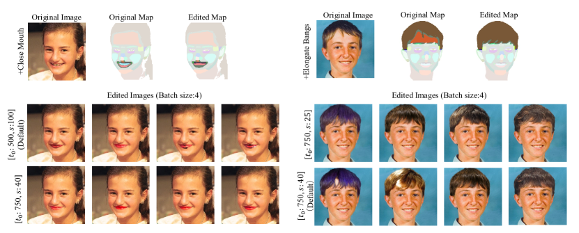
Figure 11: We show some failure cases. There are few exceptions which cannot be edited naturally on default set of $t_{0}$ and $s$. We show such edited examples obtained stochastically within batch size, which we set to 4. Both examples can produce a natural image with some of the default settings. But, in the sample shown on the left, more steps are more stable, while in the sample shown on the right, smaller scales are more stable. In these cases, the user is required to manually tune the value of $t_{0}$ and $s$ after observing the outcomes.

Table 2: We present an analysis of performance changes for the selection strategy of edited images. We investigated several selection strategies in the proposed method. (a) selecting a qualitatively superior sample, (b) selecting a quantitatively superior sample, and (c) random selection. In (c), we also report the standard deviation of each performance metric. We confirmed that the proposed method is not sensitive to the selection strategies and outperformed EditGAN in all metrics.

Method	$m$=0			whole image			$m$=1
	MAE ↓	PSNR ↑		FID ↓	IS ↑		Accuracy ↑
EditGAN	0.07485	67.24		79.67	3.765		0.8138
(a) Ours (qualitative choice)	0.01380	81.53		15.07	4.416		0.8290
(b) Ours (quantitative choice)	0.01425	81.44		15.81	4.377		0.8302
(c) Ours (random choice)	0.01393 $\pm$ 0.001742	81.59 $\pm$ 0.02958		14.62 $\pm$ 1.005	4.459 $\pm$ 0.03649		0.8195 $\pm$ 0.001742

B.2 Further Comparison with SDEdit

In SDEdit, there is a realism-faithfulness trade-off when we vary the value of $t_{0}$ [31]. Therefore, we also investigated how the edited images of our method change depending on the value of $t_{0}$. In this experiment of SDEdit, we varied the value of $t_{0}$ from 0.1 to 0.5 and corresponding total denoising steps $N$ using VP-SDE ($K$=1). Figure.10 shows several examples of the edited images. These results were obtained by selecting a qualitatively superior sample within a mini-batch for each image in both our method and SDEdit. These results support that there is a strict trade-off between faithfulness and realism in SDEdit as reported in the paper [31]. It is difficult for the users to tune $t_{0}$ manually because the appropriate $t_{0}$ varies from image to image. Also, even if the $t_{0}$ is set optimally, the proposed method can achieve more natural editing.

B.3 On the threshold to the size of the editing region

As described in Sec.4.4, we set the threshold to the size of the editing region and changed the value of $t_{0}$ based on this thresholding. In the analysis in Sec.4.4, we set 5000 pixels as the threshold, because there was a big gap in ths size of the editing region between large and small part’s manipulation. In Fig.12, we show the statistics of the number of pixels in the ROI over all datasets used in the experiments of Sec. 4.2 and Sec. B.6, which are FFHQ-34, Celeb-A, and LSUN-Cat. It demonstrates that most of the samples have a fairly small number of pixels within $m$ = 1, while the others have exceptionally large. To adopt the specific configuration to such samples with large ROI, we set the threshold to 5000. This value is not much sensitive to the performance of the proposed method as shown in Fig. 12.

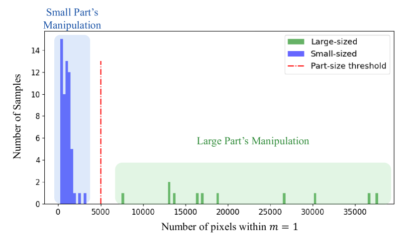
Figure 12: Statistics of the number of pixels in the ROI over all datasets used in Sec.4.2 and Sec. B.6, which are FFHQ-34, Celeb-A, and LSUN-Cat. We confirmed that this threshold is not a sensitive parameter.

B.4 Failure Cases

There were few failure cases, in which we cannot obtain natural results by the proposed method with the default setting of $t_{0}$ and $s$. We show such examples in Fig. 11. In this figure, we demonstrate the all edited images within the mini-batch, which we set to 4. The original image, the original segmentation map, and the edited map are shown in the first row, and the second and third row show the edited images with the default setting and tuned setting, respectively. From the samples shown on the left, we confirmed that images with features less observed in training data, such as teeth with orthodontics, require larger $t_{0}$, such as $t_{0}$=750, to produce naturally edited images. From the right samples, we found that setting a large value to $s$ occasionally changed hair color in some cases. In these cases, the user is required to manually tune the value of $t_{0}$ and $s$ after observing the outcomes.

B.5 On strategies for selecting edited images

In this work, we assume that the users selected the qualitatively best images among the several edited images provided by our method. Consequently, the performance of our method may depend on this selection strategy, because our method provides some variety in the edited images as shown in Fig. 11. We investigated the performance of our method with several strategies for the selection: (a) selecting a qualitatively superior sample as in Sec.4.2, (b) selecting a quantitatively superior sample in terms of the error of the segmentation map estimated from the edited images, (c) random selection. The results are shown in Table 2. In (c) we also report the standard deviation of each performance metric. We confirmed that the performance of the proposed method is not sensitive to the choice of the strategy.

B.6 Additional Results of Our Method

We present additional examples of the edited images produced by our method on FFHQ-256, LSUN-Cat and LSUN-Horse (Figs.13-19). In all examples, the original real images and the corresponding maps are shown on the left, and the edited maps and the resultant images are shown on the right. The experimental settings are the same with those in Sec.4.2 and Sec.4.3

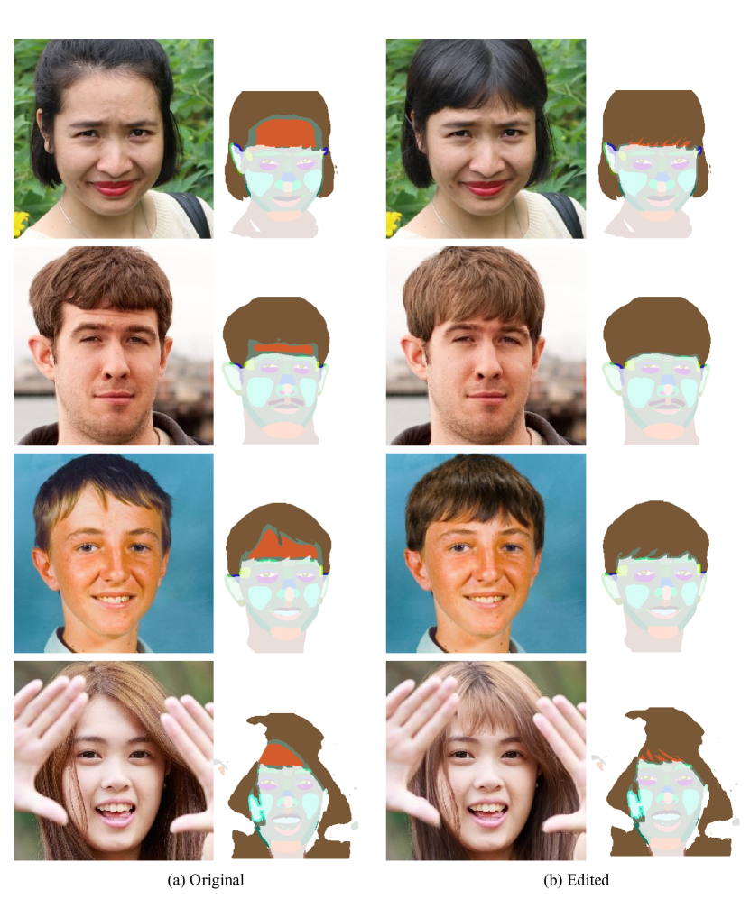
Figure 13: Hairstyle Editing.

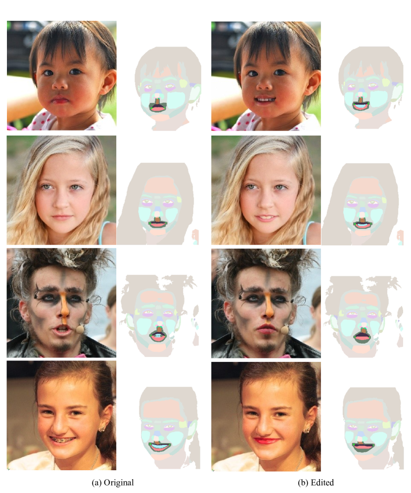
Figure 14: Mouth Editing. In these examples, we show the manipulation of ”+Open Mouth” in the top two rows and examples of ”+Open Mouth” in the bottom two rows.

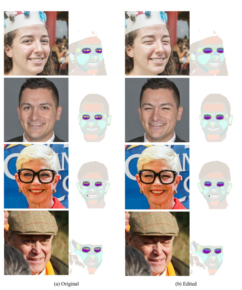
Figure 15: Closing Eyes. We show some examples of the manipulation of ”+Close Eyes”. We confirmed that eyes in glasses, eyes with shadows, etc., could also be generated naturally.

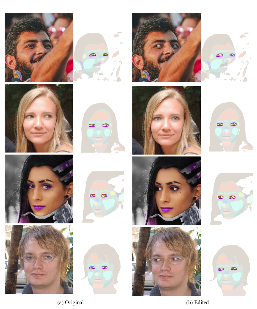
Figure 16: Moving Eyes. We demonstrate some examples corresponding to ”+Moving Eyes”.

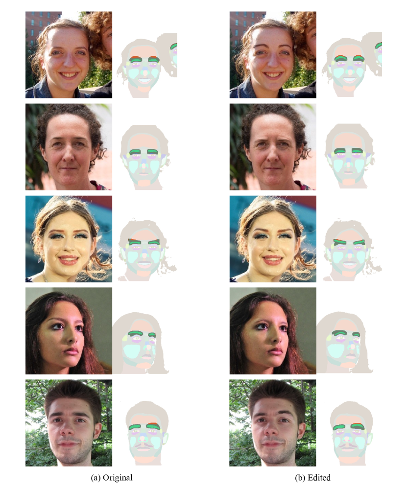
Figure 17: Eyebrow Editing. We show examples of editing that change the shape or position of eyebrows. We confirmed that the proposed method allows editing only one of the semantic-related parts (such as lift right eyebrow while keeping the left eyebrow unchanged), which EditGAN is not good at.

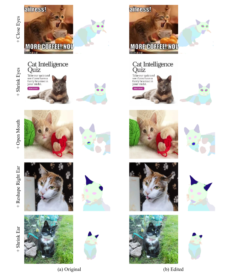
Figure 18: Editing cat images. We show some edited examples following by the written text.

Figure 19: Editing horse images. We show some edited examples following by the written text. In the above three samples, we set {$t_{0}$,$s$} = {$500$,$100$} according to the threshold setting. In the two samples below, we set $\{t_{0},s\}$=$\{800,25\}$, because this manipulation, which forces to replace some objects to background or generate some objects on background, requires a large steps as discussed in Sec.4.4. In the bottom example, the semantic editing was done, but the color was changed as described in Sec.11

References

- [1] Rameen Abdal, Yipeng Qin, and Peter Wonka. Image2stylegan: How to embed images into the stylegan latent space? 2019 IEEE/CVF International Conference on Computer Vision (ICCV), pages 4431–4440, 2019.
- [2] Rameen Abdal, Yipeng Qin, and Peter Wonka. Image2stylegan++: How to edit the embedded images? 2020 IEEE/CVF Conference on Computer Vision and Pattern Recognition (CVPR), pages 8293–8302, 2020.
- [3] Yuval Alaluf, Or Patashnik, and Daniel Cohen-Or. Restyle: A residual-based stylegan encoder via iterative refinement. 2021 IEEE/CVF International Conference on Computer Vision (ICCV), pages 6691–6700, 2021.
- [4] Yuval Alaluf, Omer Tov, Ron Mokady, Rinon Gal, and Amit H. Bermano. Hyperstyle: Stylegan inversion with hypernetworks for real image editing. 2022 IEEE/CVF Conference on Computer Vision and Pattern Recognition (CVPR), pages 18490–18500, 2022.
- [5] Omri Avrahami, Ohad Fried, and Dani Lischinski. Blended latent diffusion. ArXiv, abs/2206.02779, 2022.
- [6] Omri Avrahami, Dani Lischinski, and Ohad Fried. Blended diffusion for text-driven editing of natural images. In Proceedings of the IEEE/CVF Conference on Computer Vision and Pattern Recognition, pages 18208–18218, 2022.
- [7] Jason Bailey. The tools of generative art, from flash to neural networks. Art in America, 8, 2020.
- [8] Dmitry Baranchuk, Ivan Rubachev, Andrey Voynov, Valentin Khrulkov, and Artem Babenko. Label-efficient semantic segmentation with diffusion models. ArXiv, abs/2112.03126, 2022.
- [9] David Bau, Hendrik Strobelt, William S. Peebles, Jonas Wulff, Bolei Zhou, Jun-Yan Zhu, and Antonio Torralba. Semantic photo manipulation with a generative image prior. ACM Transactions on Graphics (TOG), 38:1 – 11, 2019.
- [10] David Bau, Jun-Yan Zhu, Hendrik Strobelt, Bolei Zhou, Joshua B. Tenenbaum, William T. Freeman, and Antonio Torralba. Gan dissection: Visualizing and understanding generative adversarial networks. ArXiv, abs/1811.10597, 2019.
- [11] Andrew Brock, Jeff Donahue, and Karen Simonyan. Large scale gan training for high fidelity natural image synthesis. arXiv preprint arXiv:1809.11096, 2018.
- [12] Shu-Yu Chen, Wanchao Su, Lin Gao, Shi hong Xia, and Hongbo Fu. Deepfacedrawing: deep generation of face images from sketches. ACM Trans. Graph., 39:72, 2020.
- [13] Jooyoung Choi, Sungwon Kim, Yonghyun Jeong, Youngjune Gwon, and Sungroh Yoon. Ilvr: Conditioning method for denoising diffusion probabilistic models. 2021 IEEE/CVF International Conference on Computer Vision (ICCV), pages 14347–14356, 2021.
- [14] Jooyoung Choi, Jungbeom Lee, Chaehun Shin, Sungwon Kim, Hyunwoo J. Kim, and Sung-Hoon Yoon. Perception prioritized training of diffusion models. 2022 IEEE/CVF Conference on Computer Vision and Pattern Recognition (CVPR), pages 11462–11471, 2022.
- [15] Florinel-Alin Croitoru, Vlad Hondru, Radu Tudor Ionescu, and Mubarak Shah. Diffusion models in vision: A survey. ArXiv, abs/2209.04747, 2022.
- [16] Prafulla Dhariwal and Alex Nichol. Diffusion models beat gans on image synthesis. ArXiv, abs/2105.05233, 2021.
- [17] Rinon Gal, Or Patashnik, Haggai Maron, Gal Chechik, and Daniel Cohen-Or. Stylegan-nada: Clip-guided domain adaptation of image generators. ArXiv, abs/2108.00946, 2021.
- [18] Ian J Goodfellow, Jean Pouget-Abadie, Mehdi Mirza, Bing Xu, David Warde-Farley, Sherjil Ozair, Aaron Courville, and Yoshua Bengio. Generative adversarial networks. In Proceedings of the International Conference on Neural Information Processing Systems, pages 2672–2680, 2014.
- [19] Martin Heusel, Hubert Ramsauer, Thomas Unterthiner, Bernhard Nessler, and Sepp Hochreiter. Gans trained by a two time-scale update rule converge to a local nash equilibrium. In NIPS, 2017.
- [20] Jonathan Ho, Ajay Jain, and P. Abbeel. Denoising diffusion probabilistic models. ArXiv, abs/2006.11239, 2020.
- [21] Tero Karras, Timo Aila, Samuli Laine, and Jaakko Lehtinen. Progressive growing of gans for improved quality, stability, and variation. ArXiv, abs/1710.10196, 2018.
- [22] Tero Karras, Samuli Laine, and Timo Aila. A style-based generator architecture for generative adversarial networks. 2019 IEEE/CVF Conference on Computer Vision and Pattern Recognition (CVPR), pages 4396–4405, 2019.
- [23] Tero Karras, Samuli Laine, Miika Aittala, Janne Hellsten, Jaakko Lehtinen, and Timo Aila. Analyzing and improving the image quality of stylegan. 2020 IEEE/CVF Conference on Computer Vision and Pattern Recognition (CVPR), pages 8107–8116, 2020.
- [24] Gwanghyun Kim, Taesung Kwon, and Jong-Chul Ye. Diffusionclip: Text-guided diffusion models for robust image manipulation. 2022 IEEE/CVF Conference on Computer Vision and Pattern Recognition (CVPR), pages 2416–2425, 2022.
- [25] Diederik P. Kingma and Jimmy Ba. Adam: A method for stochastic optimization. CoRR, abs/1412.6980, 2015.
- [26] Diederik P Kingma and Max Welling. Auto-encoding variational bayes. arXiv preprint arXiv:1312.6114, 2013.
- [27] Gihyun Kwon and Jong-Chul Ye. Clipstyler: Image style transfer with a single text condition. 2022 IEEE/CVF Conference on Computer Vision and Pattern Recognition (CVPR), pages 18041–18050, 2022.
- [28] Mingi Kwon, Jaeseok Jeong, and Youngjung Uh. Diffusion models already have a semantic latent space. ArXiv, abs/2210.10960, 2022.
- [29] Cheng-Han Lee, Ziwei Liu, Lingyun Wu, and Ping Luo. Maskgan: Towards diverse and interactive facial image manipulation. 2020 IEEE/CVF Conference on Computer Vision and Pattern Recognition (CVPR), pages 5548–5557, 2020.
- [30] Huan Ling, Karsten Kreis, Daiqing Li, Seung Wook Kim, Antonio Torralba, and Sanja Fidler. Editgan: High-precision semantic image editing. In NeurIPS, 2021.
- [31] Chenlin Meng, Yang Song, Jiaming Song, Jiajun Wu, Junyan Zhu, and Stefano Ermon. Sdedit: Image synthesis and editing with stochastic differential equations. ArXiv, abs/2108.01073, 2021.
- [32] Jacob Menick and Nal Kalchbrenner. Generating high fidelity images with subscale pixel networks and multidimensional upscaling. arXiv preprint arXiv:1812.01608, 2018.
- [33] Takuya Narihira, Javier Alonsogarcia, Fabien Cardinaux, Akio Hayakawa, Masato Ishii, Kazunori Iwaki, Thomas Kemp, Yoshiyuki Kobayashi, Lukas Mauch, Akira Nakamura, et al. Neural network libraries: A deep learning framework designed from engineers’ perspectives. arXiv preprint arXiv:2102.06725, 2021.
- [34] Alex Nichol and Prafulla Dhariwal. Improved denoising diffusion probabilistic models. ArXiv, abs/2102.09672, 2021.
- [35] Alex Nichol, Prafulla Dhariwal, Aditya Ramesh, Pranav Shyam, Pamela Mishkin, Bob McGrew, Ilya Sutskever, and Mark Chen. Glide: Towards photorealistic image generation and editing with text-guided diffusion models. In ICML, 2022.
- [36] Taesung Park, Ming-Yu Liu, Ting-Chun Wang, and Jun-Yan Zhu. Semantic image synthesis with spatially-adaptive normalization. 2019 IEEE/CVF Conference on Computer Vision and Pattern Recognition (CVPR), pages 2332–2341, 2019.
- [37] Adam Paszke, Sam Gross, Francisco Massa, Adam Lerer, James Bradbury, Gregory Chanan, Trevor Killeen, Zeming Lin, Natalia Gimelshein, Luca Antiga, et al. Pytorch: An imperative style, high-performance deep learning library. Advances in neural information processing systems, 32, 2019.
- [38] Or Patashnik, Zongze Wu, Eli Shechtman, Daniel Cohen-Or, and Dani Lischinski. Styleclip: Text-driven manipulation of stylegan imagery. 2021 IEEE/CVF International Conference on Computer Vision (ICCV), pages 2065–2074, 2021.
- [39] Antoine Plumerault, Hervé Le Borgne, and Céline Hudelot. Controlling generative models with continuous factors of variations. ArXiv, abs/2001.10238, 2020.
- [40] Konpat Preechakul, Nattanat Chatthee, Suttisak Wizadwongsa, and Supasorn Suwajanakorn. Diffusion autoencoders: Toward a meaningful and decodable representation. 2022 IEEE/CVF Conference on Computer Vision and Pattern Recognition (CVPR), pages 10609–10619, 2022.
- [41] Danilo Rezende and Shakir Mohamed. Variational inference with normalizing flows. In International conference on machine learning, pages 1530–1538. PMLR, 2015.
- [42] Elad Richardson, Yuval Alaluf, Or Patashnik, Yotam Nitzan, Yaniv Azar, Stav Shapiro, and Daniel Cohen-Or. Encoding in style: a stylegan encoder for image-to-image translation. 2021 IEEE/CVF Conference on Computer Vision and Pattern Recognition (CVPR), pages 2287–2296, 2021.
- [43] Chitwan Saharia, William Chan, Huiwen Chang, Chris A. Lee, Jonathan Ho, Tim Salimans, David J. Fleet, and Mohammad Norouzi. Palette: Image-to-image diffusion models. ACM SIGGRAPH 2022 Conference Proceedings, 2022.
- [44] Tim Salimans, Ian J. Goodfellow, Wojciech Zaremba, Vicki Cheung, Alec Radford, and Xi Chen. Improved techniques for training gans. ArXiv, abs/1606.03498, 2016.
- [45] Yujun Shen, Jinjin Gu, Xiaoou Tang, and Bolei Zhou. Interpreting the latent space of gans for semantic face editing. 2020 IEEE/CVF Conference on Computer Vision and Pattern Recognition (CVPR), pages 9240–9249, 2020.
- [46] Yujun Shen, Ceyuan Yang, Xiaoou Tang, and Bolei Zhou. Interfacegan: Interpreting the disentangled face representation learned by gans. IEEE Transactions on Pattern Analysis and Machine Intelligence, 44:2004–2018, 2022.
- [47] Jascha Narain Sohl-Dickstein, Eric A. Weiss, Niru Maheswaranathan, and Surya Ganguli. Deep unsupervised learning using nonequilibrium thermodynamics. ArXiv, abs/1503.03585, 2015.
- [48] Jiaming Song, Chenlin Meng, and Stefano Ermon. Denoising diffusion implicit models. ArXiv, abs/2010.02502, 2021.
- [49] Yang Song and Stefano Ermon. Generative modeling by estimating gradients of the data distribution. ArXiv, abs/1907.05600, 2019.
- [50] Yang Song, Jascha Narain Sohl-Dickstein, Diederik P. Kingma, Abhishek Kumar, Stefano Ermon, and Ben Poole. Score-based generative modeling through stochastic differential equations. ArXiv, abs/2011.13456, 2021.
- [51] Omer Tov, Yuval Alaluf, Yotam Nitzan, Or Patashnik, and Daniel Cohen-Or. Designing an encoder for stylegan image manipulation. ACM Transactions on Graphics (TOG), 40:1 – 14, 2021.
- [52] Aäron Van Den Oord, Nal Kalchbrenner, and Koray Kavukcuoglu. Pixel recurrent neural networks. In International conference on machine learning, pages 1747–1756. PMLR, 2016.
- [53] Zongze Wu, Dani Lischinski, and Eli Shechtman. Stylespace analysis: Disentangled controls for stylegan image generation. 2021 IEEE/CVF Conference on Computer Vision and Pattern Recognition (CVPR), pages 12858–12867, 2021.
- [54] Weihao Xia, Yujiu Yang, Jing Xue, and Baoyuan Wu. Tedigan: Text-guided diverse face image generation and manipulation. 2021 IEEE/CVF Conference on Computer Vision and Pattern Recognition (CVPR), pages 2256–2265, 2021.
- [55] Weihao Xia, Yulun Zhang, Yujiu Yang, Jing-Hao Xue, Bolei Zhou, and Ming-Hsuan Yang. Gan inversion: A survey. ArXiv, abs/2101.05278, 2022.
- [56] Yanbo Xu, Yueqin Yin, Liming Jiang, Qianyi Wu, Chengyao Zheng, Chen Change Loy, Bo Dai, and Wayne Wu. Transeditor: Transformer-based dual-space gan for highly controllable facial editing. 2022 IEEE/CVF Conference on Computer Vision and Pattern Recognition (CVPR), pages 7673–7682, 2022.
- [57] Fisher Yu, Yinda Zhang, Shuran Song, Ari Seff, and Jianxiong Xiao. Lsun: Construction of a large-scale image dataset using deep learning with humans in the loop. ArXiv, abs/1506.03365, 2015.
- [58] Yuxuan Zhang, Huan Ling, Jun Gao, K. Yin, Jean-Francois Lafleche, Adela Barriuso, Antonio Torralba, and Sanja Fidler. Datasetgan: Efficient labeled data factory with minimal human effort. 2021 IEEE/CVF Conference on Computer Vision and Pattern Recognition (CVPR), pages 10140–10150, 2021.
- [59] Jiapeng Zhu, Yujun Shen, Deli Zhao, and Bolei Zhou. In-domain gan inversion for real image editing. ArXiv, abs/2004.00049, 2020.