Kronecker-structured Covariance Models for Multiway DataThis work was supported in part by the SOLSTICE Drive Center funded by NASA and National Science Foundation under grant 80NSSC20K0600, the Army Research Office under grants W911NF1910269 and W911NF1510479, and by the National Nuclear Security Administration under grant DE-NA0003921.

Abstract

Many applications produce multiway data of exceedingly high dimension. Modeling such multi-way data is important in multichannel signal and video processing where sensors produce multi-indexed data, e.g. over spatial, frequency, and temporal dimensions. We will address the challenges of covariance representation of multiway data and review some of the progress in statistical modeling of multiway covariance over the past two decades, focusing on tensor-valued covariance models and their inference. We will illustrate through a space weather application: predicting the evolution of solar active regions over time.

, , and

1 Introduction

Probabilistic modeling of data is ubiquitous in statistics and machine learning, and arguably, estimating dependencies across covariates is one of the most fundamental modeling tasks. While first order “mean field” analysis can describe typical mean behavior of covariates, higher order analysis is required to capture interactions between covariates. Among the latter, covariance estimation is a second order analysis that has been extensively studied for empirically estimating the covariance or the inverse covariance (precision) matrix from multivariate data. Besides being of interest in their own right, covariance estimates are often a prerequisite in other applications, including: dimensionality reduction; multivariate clustering; supervised classification; linear prediction; and model selection [42, 63, 101, 5, 24, 79, 80, 81].

A striking feature of many modern datasets is their high-dimensionality and multiway nature, often involving a huge number of multi-indexed variables represented as tensor-valued data [46, 48]. Second order analysis of such tensor-valued data poses significant modeling and computational challenges due to the intrinsically high computational complexity of manipulating tensor representations [35]. To overcome these challenges, several methodological approaches have been developed over the past 50 years that reduce model complexity by imposing sparse or low-dimensional dependency structures in the covariance or inverse covariance. These include Kronecker generalizations of PCA (Kronecker PCA) [84, 30] and the matrix normal model [19], where the covariates are multivariate normal with multiway covariance structure modeled as a Kronecker product of matrices of much lower dimension. These Kronecker representations of covariance can have Kronecker factors that are either dense [22, 95] or sparse [2, 85].

The introduction of such parsimoniously structured tensor covariance models, and fast iterative computational algorithms for inferring these models, have made tensor covariance models more practical for many applications. In particular, such models have been applied to image classification [25], spatio-temporal image processing [30, 32, 65, 20], bioinformatics [83, 31, 82, 21], atmospheric science [54, 33], neuroscience [91, 78, 7], medical imaging [58, 57], and digital advertising [34]. Several other applications of multiway covariance models are discussed in the unpublished survey [76].

In this article, we survey some of the recent advances in second order analysis of multiway data. The focus is on Kronecker structured representations and approximations to multiway covariance. After introducing some notation in Section 2, we describe how multiway covariance structure arises in different applications, including in linear prediction of dynamic processes whose evolution is governed by differential equations. We then overview recent approaches to Kronecker modeling and estimation of multiway covariance and inverse covariance in Section 3. In Section 4, we summarize and compare these Kronecker models and estimators based on their theoretical performance properties and a numerical comparison study. The numerical study focuses on model comparison for an important application in the domain of space weather: prediction of solar active region evolution over time. In Section 5, we conclude the paper with a few open research directions in second order multiway data modeling. A software package [92] accompanies this survey with code implementing the methods described herein.

This survey is intended to complement previous surveys on aspects of high dimensional covariance modeling important to practitioners. These include surveys on robust structured covariance estimation [96, 44] and regularized covariance estimation [69, 49, 13]. Here, we focus on the class of Kronecker structured covariance models.

2 Background

2.1 Notation

Throughout the paper, scalars are denoted by lowercase letters, vectors by boldface lowercase letters, and matrices by boldface capital letters. All matrix and vector quantities are assumed to be real valued, although all the multiway covariance models discussed in this paper straightforwardly generalize to complex valued data. For a matrix $\mathbf{A}=(\mathbf{A}_{i,j})\in\mathbb{R}^{d\times d}$, the spectral norm is denoted as $\|\mathbf{A}\|_{2}$, the Frobenius norm as $\|\mathbf{A}\|_{F}$, and the nuclear norm as $\|\mathbf{A}\|_{*}$. We define $\|\mathbf{A}\|_{1,\text{off}}:=\sum_{i\neq j}|\mathbf{A}_{i,j}|$ as its off-diagonal $\ell_{1}$ norm. For tensor algebra, we adopt the notations used by Kolda and Bader [46]. $K$-th order tensors are denoted by boldface Euler script letters, e.g, $\bm{\mathcal{X}}\in{\mathbb{R}}^{d_{1}\times\dots\times d_{K}}$, with the $(i_{1},\dots,i_{K})$-th element denoted as $\bm{\mathcal{X}}_{i_{1},\dots,i_{K}}$. A fiber of a tensor is a higher order analogue of a row or a column of a matrix. It is obtained by fixing all but one of the indices of the tensor. The vectorization of $\bm{\mathcal{X}}$, denoted as $\operatorname{vec}(\bm{\mathcal{X}})$, stacks the entries of the tensor into a $d$-dimensional column vector $(\bm{\mathcal{X}}_{1,1,\dots,1},\bm{\mathcal{X}}_{2,1,\dots,1},\dots,\bm{\mathcal{X}}_{d_{1},d_{2},\dots,d_{k}})^{T}$, where $d=\prod_{k=1}^{K}d_{k}$. Matricization, also known as unfolding, is the process of transforming a tensor into a matrix. The mode-$k$ matricization of a tensor $\bm{\mathcal{X}}$, denoted by $\bm{\mathcal{X}}_{(k)}$, arranges the mode-$k$ fibers to be the columns of the resulting matrix. The $k$-mode product of a tensor $\bm{\mathcal{X}}\in{\mathbb{R}}^{d_{1}\times\dots\times d_{K}}$ and a matrix $\mathbf{A}\in{\mathbb{R}}^{J\times d_{k}}$, denoted as $\bm{\mathcal{X}}\times_{k}\mathbf{A}$, is a tensor of size $d_{1}\times\dots\times d_{k-1}\times J\times d_{k+1}\times\dots d_{K}$, with entries defined as $(\bm{\mathcal{X}}\times_{k}\mathbf{A})_{i_{1},\dots,i_{k-1},j,i_{k+1},\dots,i_{K}}:=\sum_{i_{k}=1}^{d_{k}}\bm{\mathcal{X}}_{i_{1},\dots,i_{K}}A_{j,i_{k}}$. We define the $K$-way Kronecker product (KP) as $\bigotimes_{k=1}^{K}\mathbf{A}_{k}=\mathbf{A}_{1}\otimes\cdots\otimes\mathbf{A}_{K}$, and the $K$-way Kronecker sum (KS) as $\bigoplus_{k=1}^{K}\mathbf{A}_{k}=\mathbf{A}_{1}\oplus\dots\oplus\mathbf{A}_{K}=\sum_{k=1}^{K}\mathbf{I}_{[d_{1:k-1}]}\otimes\mathbf{A}_{k}\otimes\mathbf{I}_{[d_{k+1:K}]}$, where $\mathbf{I}_{[d_{k:\ell}]}=\mathbf{I}_{d_{k}}\otimes\dots\otimes\mathbf{I}_{d_{\ell}}$. For the case of $K=2$, $\mathbf{A}_{1}\oplus\mathbf{A}_{2}=\mathbf{A}_{1}\otimes\mathbf{I}_{d_{2}}+\mathbf{I}_{d_{1}}\otimes\mathbf{A}_{2}$.

Statistical convergence rate will be denoted by the $O_{P}(\cdot)$ notation, which is defined as follows. Consider a sequence of real random variables $\{X_{n}\}_{n\in\mathbb{N}}$ defined on a probability space $(\Omega,\mathcal{F},P)$ and a deterministic (positive) sequence of reals $\{b_{n}\}_{n\in\mathbb{N}}$. By $X_{n}=O_{P}(1)$ is meant: $\sup_{n\in\mathbb{N}}P(|X_{n}|>K)\rightarrow 0$ as $K\rightarrow\infty$, where $X_{n}$ is a sequence indexed by $n$. The notation $X_{n}=O_{P}(b_{n})$ is equivalent to $\frac{X_{n}}{b_{n}}=O_{P}(1)$. By $X_{n}=o_{p}(1)$ is meant $P(|X_{n}|>\epsilon)\rightarrow 0$ as $n\rightarrow\infty$ for any $\epsilon>0$. By $\lambda_{n}\asymp b_{n}$ is meant $c_{1}\leq\frac{\lambda_{n}}{b_{n}}\leq c_{2}$ for all $n$, where $c_{1},c_{2}>0$ are absolute constants. The asymptotic notation $a_{n}=O(b_{n})$ means $\lim\sum_{b\rightarrow\infty}|\frac{a_{n}}{b_{n}}|\leq C$ for some constant $C>0$, while $c_{n}=\Omega(d_{n})$ means $\lim\inf_{n\rightarrow\infty}|\frac{c_{n}}{d_{n}}|\geq C^{\prime}$ for some constant $C^{\prime}>0$.

2.2 Multiway Data

Multiway data frame

Multiway data are data that are indexed over multiple domains, called modes, and can be represented as a tensor-valued data frame. The number of modes is called the order of the tensor. Examples of multiway data include 3D images of the brain, where the modes are the 3 spatial dimensions, and spatio-temporal weather imaging data, a set of image sequences represented as 2 spatial modes and 1 temporal mode. One can also obtain a multiway data by stacking independent, identically distributed data samples.

Multiway patterned covariance matrix

Given a multiway data tensor of order $K$, the covariance matrix of the vectorized data has a special patterned structure. For instance, suppose that $\mathbf{X}\in\mathbb{R}^{d_{1}\times d_{2}}$ is a multiway data frame of order $2$, (i.e., a matrix). Then the covariance matrix of $\operatorname{vec}(\mathbf{X})$ is a $d_{1}d_{2}$ by $d_{1}d_{2}$ matrix $\mathbf{\Sigma}=(\Sigma_{ij})$ that corresponds to the covariance of the $i$-th and the $j$-th rows of $\mathbf{X}$. See Figure 1 for a visual illustration. As a special case, if the rows of $\mathbf{X}$ are independent and identically distributed with $d_{2}\times d_{2}$ covariance $\mathbf{\Sigma}_{d_{2}}$, then ${}\mathrm{cov}(\mathbf{X})=\mathbf{I}_{d_{1}}\otimes\mathbf{\Sigma}_{d_{2}}$.

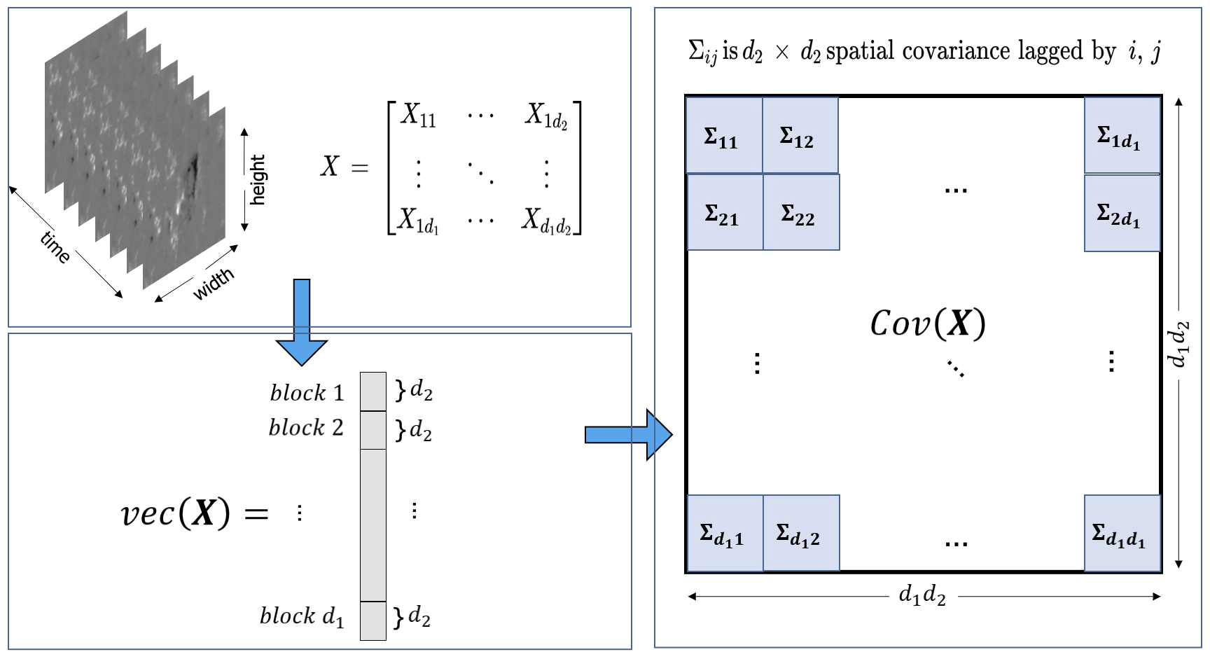
Figure 1: Multiway data and patterned covariance.

Utility of multiway data for prediction

Arguably, regression analysis is one of the most straightforward approaches for prediction as it attempts to estimate the relation between the covariates and the response variable. Despite its long and fruitful history, traditional regression techniques often fall short of handling multiway data encountered in modern applications, due to the ultrahigh data dimensionality as well as complex data structure. Recently, several tensor regression models were proposed to exploit the special structure of tensor covariates [105, 34] or of tensor responses [71, 53, 106]. These models try to utilize the sparse and low-rank structures in the tensors – either in the regression coefficient tensor or the response tensor – to boost performance on the regression task by reducing the number of free parameters. Similarly, in Section 4.3, we demonstrate the utility of sparse precision/covariance matrices in linear prediction for tensor-valued data.

2.3 Multiway covariance representations for diffusion processes

While multiway representations have been successfully applied to many different types of data, they are particularly interpretable when modeling data generated from physical diffusion processes. In particular, consider a random process $u$ whose sample paths obey a partial differential equations of the form

$$\mathcal{D}u =f\quad\text{in }\Omega,$$ (1)

$$u =g\quad\text{on }\partial\Omega,$$

where $u$ is the unknown physical process, $f$ is the driving process (e.g., white Gaussian noise), $g$ is the function value of $u$ on the boundary, $\mathcal{D}$ is some differential operator (e.g, a Laplacian or an Euler-Lagrange operator), and $\Omega$ is the domain. After finite difference discretization over the domain $\Omega$, the model is equivalent to (ignoring discretization error) the matrix equation

$${\mathbf{D}}{\mathbf{u}}=\mathbf{f}.$$

Here, ${\mathbf{D}}$ is a sparse matrix since $\mathcal{D}$ is a differential operator. Additionally, as shown below, ${\mathbf{D}}$ admits the Kronecker structure as a mixture of Kronecker sums and Kronecker products.

The matrix ${\mathbf{D}}$ reduces to a Kronecker sum when $\mathcal{D}$ involves no mixed derivatives. As an example, we consider the Poisson equation, an elliptical PDE that governs many physical processes including electromagnetic induction, heat transfer, and convection. On a rectangular region $\Omega=(0,d_{1})\times(0,d_{2})$ in the 2D Cartesian plane, the Poisson equation with homogeneous Dirichlet boundary condition is expressed as

$$\mathcal{D}u=(\partial^{2}_{x}+\partial^{2}_{y})u =f\quad\text{in }\Omega,$$ (2)

$$u =0\quad\text{on }\partial\Omega$$

where $f:\Omega\to{\mathbb{R}}$ is the given source function and $u:\Omega\to{\mathbb{R}}$ is the unknown process of interest. Using the finite difference method with a square mesh grid with unit spacing, the unknown and the source can be expressed as $d_{1}$-by-$d_{2}$ matrices, ${\mathbf{U}}$ and ${\mathbf{F}}$, respectively, that are related to each other via

$$U_{i+1,j}+U_{i-1,j}+U_{i,j+1}+U_{i,j-1}-4U_{i,j}=F_{i,j}$$ (3)

for any interior grid point $(i,j)$. Defining $n$-by-$n$ square matrix

$$\mathbf{A}_{n}=\begin{bmatrix}2&-1&&\\ -1&2&\ddots&\\ &\ddots&\ddots&-1\\ &&-1&2\end{bmatrix},$$

the above relation can be expressed as the (vectorized) Sylvester equation with $K=2$:

$$({\mathbf{A}}_{d_{1}}\oplus{\mathbf{A}}_{d_{2}}){\mathbf{u}}={\mathbf{f}},$$ (4)

where ${\mathbf{u}}=\operatorname{vec}({\mathbf{U}})$, ${\mathbf{f}}=\operatorname{vec}({\mathbf{F}})$. Note that $\mathbf{A}_{n}$ is tridiagonal. In the case where $\mathbf{f}$ is white noise with variance $\sigma^{2}$, the inverse covariance matrix of ${\mathbf{u}}$ has the form ${}\mathrm{cov}^{-1}({\mathbf{u}})=\sigma^{-2}({\mathbf{A}}_{d_{1}}\oplus{\mathbf{A}}_{d_{2}})^{T}({\mathbf{A}}_{d_{1}}\oplus{\mathbf{A}}_{d_{2}})$ and hence sparse.

More generally, any physical process generated from Equation (1) also has sparse inverse covariance matrices due to the sparsity of general discretized differential operators. Note that similar connections between continuous state physical processes and sparse “discretized” statistical models have been established by Lindgren, Rue and Lindström [56], who elucidated a link between Gaussian fields and Gauss Markov Random Fields via stochastic partial differential equations.

In some applications, e.g. weather forecasting and multivariate time series, the data frame $\mathbf{X}$ can be modeled as having been generated by an underlying dynamical process obeying the aforementioned physical diffusion model. This model can be used for various tasks such as forecasting, classification, and two-sample comparison. For example, when the dynamical model is of known linear form, the Kalman filter can be used for these tasks [8]. In the case of non-linear dynamics the ensemble Kalman filter (EnKF) [23] is applicable. Recently, a sparsity-penalized EnKF was introduced for modeling non-linear state dynamics [39]. This EnKF was implemented with a sparse inverse covariance estimator in order to stabilize the error covariance update of the Kalman Filter. When the state is high dimensional and tensor-valued, [89] used Kronecker-structured models for the (inverse) covariance and demonstrated improvements in tracking certain classes of dynamical models. A similar application of Kronecker covariance modeling will be further illustrated in Section 4.2.

3 Multiway Covariance Models

In this section, we survey several covariance models for multiway data and review associated estimation algorithms that have been introduced in the literature. The common assumption of these models is that the multimodal covariance (or inverse covariance) of multiway data has a factorized representation involving a Kronecker product or a Kronecker sum of smaller matrices, or as a linear combination thereof. Each of the smaller matrices corresponds to a single mode of data and these are often interpreted as mode-wise (inverse) covariances. The models and the algorithms reviewed in this section are summarized in Table 1.

Table 1: Overview of the models and the algorithms reviewed in Section 3. Here, $\Sigma$ and $\Omega$ denote the covariance and the inverse covariance (precision), respectively. For the sake of brevity, the model in the second column is described for $K=2$.

	Model	Algorithm	Note
KP-Covariance (Section 3.2)	${\bm{\Sigma}}=\sum_{l=1}^{r}{\mathbf{A}}_{l}\otimes{\mathbf{B}}_{l}$	KPCA [84]	Algorithm requires $K=2$
		Robust KPCA [31]	Algorithm requires $K=2$
		AdaKron [52]	Analysis restricted to $K=2$
		TRCM [2]	Analysis restricted to $K=2$
		Gemini [104]	Analysis restricted to $K=2$
KP-Precision (Section 3.3)	${\bm{\Omega}}={\mathbf{A}}\otimes{\mathbf{B}}$	KGlasso [2, 85]	Analysis restricted to $K=2$
		Tlasso [59]	Applicable to $K\geq 2$
KS-Precision (Section 3.4)	${\bm{\Omega}}={\mathbf{A}}\oplus{\mathbf{B}}$	Teralasso [33]	Applicable to $K\geq 2$
		BiGlasso [43]	Analysis restricted to $K=2$
Sylvester GM (Section 3.5)	${\bm{\Omega}}=({\mathbf{A}}\oplus{\mathbf{B}})^{2}$	SyGlasso [91]	Applicable to $K\geq 2$
		SG-PALM [90]	Applicable to $K\geq 2$

3.1 The Kronecker Product Covariance Model

For a $K$-mode tensor-valued data frame, the Kronecker product (KP) model of its covariance matrix ${\bm{\Sigma}}$ is

$${\bm{\Sigma}}={\bm{\Sigma}}_{1}\otimes\dots\otimes{\bm{\Sigma}}_{K}$$ (5)

where ${\bm{\Sigma}}_{k}\in{\mathbb{R}}^{d_{k}\times d_{k}},k=1,\ldots,K$ are symmetric positive-semidefinite matrices, which are called the Kronecker factors of ${\bm{\Sigma}}$.

The KP model with $K=2$ imposes a simple two-way covariance representation recast as ${\bm{\Sigma}}={\mathbf{A}}\otimes{\mathbf{B}}$, arguably the simplest non-trivial one. Then, under this model, each $d_{2}\times d_{2}$ block $[{\bm{\Sigma}}]_{ij}$ of the $d_{1}d_{2}\times d_{1}d_{2}$ patterned covariance matrix ${\bm{\Sigma}}$ shown in Figure 1 is the same matrix, namely $[{\bm{\Sigma}}]_{ij}={\mathbf{B}}$, up to a multiplicative factor. Despite its apparent simplicity, the KP model with $K=2$ has been used effectively in many different applications, including spatio-temporal data frames arising in MIMO wireless communications [100, 95], geostatistics [16], genomics [98, 38], face recognition [102], and recommender systems [2].

The KP model was introduced by Dawid [19] in the context of the matrix normal distribution for data with $K=2$ tensor modes. An alternating optimization algorithm for maximum likelihood estimation (MLE) of the $K=2$ Kronecker factors was introduced by Mardia and Goodall [61] and analyzed by Dutilleul [22]. A different approach based on the covariance matching principle was taken by Strobach [75], who cast the problem of estimating the $K=2$ Kronecker factors as a minimum Frobenius norm covariance matching problem:

$$\min_{{\mathbf{A}},{\mathbf{B}}}\|{\mathbf{S}}-{\mathbf{A}}\otimes{\mathbf{B}}\|_{F}^{2}.$$ (6)

Using the fact that the matrix Frobenius norm is invariant to permutation of the entries, the above optimization (6) boils down to finding the rank-one approximation to the matrix ${\mathcal{R}}({\mathbf{S}})$, where ${\mathcal{R}}$ is the rearrangement-permutation operator that maps the square matrix ${\mathbf{S}}\in{\mathbb{R}}^{d_{1}d_{2}\times d_{1}d_{2}}$ to a rectangular matrix ${\mathcal{R}}({\mathbf{S}})\in{\mathbb{R}}^{d_{1}^{2}\times d_{2}^{2}}$ [87]. The minimizers of (6) can thus be expressed in closed form using the left and right principal components ${\mathbf{u}}$ and ${\mathbf{v}}$ of ${\mathcal{R}}({\mathbf{S}})$ as $\widehat{{\mathbf{A}}}={\mathcal{R}}^{-1}({\mathbf{u}})$ and $\widehat{{\mathbf{B}}}={\mathcal{R}}^{-1}({\mathbf{v}})$, and the resultant estimator can be represented as $\widehat{{\bm{\Sigma}}}=\widehat{{\mathbf{A}}}\otimes\widehat{{\mathbf{B}}}$. Compared to the MLE, this least square estimate does not require an iterative algorithm, but is generally not asymptotically efficient. A weighted Frobenius norm formulation based on (6) was considered by Werner, Jansson and Stoica [95], leading to an asympotically efficient estimator under the matrix normal assumption.

KP models with $K>2$ also arise in applications and are explored in the literature. Mardia and Goodall [61] considered a spatio-temporal multivariate environmental monitoring data set and adopted a KP covariance with $K=3$. They were the first to propose a maximum likelihood estimation via triple iteration. As there were insufficient replicates, they simplified the model by assuming the temporal components were statistically independent. Galecki [26] discussed five 3-way KP models with different combinations of covariance factor structures of identity, compound symmetry, AR(1), unstructured. Akdemir and Gupta [1] provided a heuristic method for $K\geq 2$, generalizing the flip-flop method originally proposed for matrices. The convergence of the algorithm was empirically verified using simulations with $K$ up to 4, and using real world data with $K$ up to 3. Hoff [36] discussed maximum likelihood estimation and Bayesian estimation for tensor normal models for general $K$, the latter approach verified on a 4-way international trade dataset. We note here that, in both Hoff [36] and Ohlson, Ahmad and Von Rosen [67], the KP model was referred to as the “separable covariance” model. An empirical study of the three-stage iterative algorithm for MLE of KP structured covariance with $K=3$ was given by Manceur and Dutilleul [60], who provided numerical and simulation results showing convergence of the algorithm. Pouryazdian, Beheshti and Krishnan [70]) proposed to select the order of Canonical Decomposition (CANDECOMP) in modeling 3-way data under the assumption that the noise covariance is a KP model with $K=3$ modes, justified by the structure of electroencephalogram (EEG) data spanning the time, frequency, and space dimensions.

3.2 Kronecker Covariance Decomposition and Kronecker PCA

There is a less restrictive model than (5) that approximates the covariance as a sum of several Kronecker products. For example, when $K=2$, the covariance under this model is expressed as

$${\bm{\Sigma}}=\sum_{l=1}^{r}{\mathbf{A}}_{l}\otimes{\mathbf{B}}_{l},$$ (7)

where $r\geq 1$ is a positive integer, ${\mathbf{A}}_{l}\in{\mathbb{R}}^{d_{1}\times d_{1}}$ and ${\mathbf{B}}_{l}\in{\mathbb{R}}^{d_{2}\times d_{2}}$ for all $1\leq l\leq r$. The sum of Kronecker product representation (7) is universal in the sense that any matrix ${\bm{\Sigma}}\in{\mathbb{R}}^{d_{1}d_{2}\times d_{1}d_{2}}$ can be expressed as a sum of $r$ Kronecker products with $r\leq\min\{d_{1}^{2},d_{2}^{2}\}$ in view of SVD, cf. Van Loan and Pitzianis [87, Section 2]. Indeed, even when $K\geq 3$, every tensor ${\bm{\Sigma}}\in{\mathbb{R}}^{d\times d}$ can be represented by a sum of Kronecker products ${\bm{\Sigma}}=\sum_{l=1}^{r}{\mathbf{A}}^{(1)}_{l}\otimes\dots\otimes{\mathbf{A}}^{(K)}_{l}$ where $d=\prod_{k=1}^{K}$ and ${\mathbf{A}}^{(k)}_{l}\in{\mathbb{R}}^{d_{k}\times d_{k}}$ for all $k\in[K]$ and $l\in[r]$. The minimum positive integer $r$ such that ${\bm{\Sigma}}$ admits a representation of the form (7) is called the (tensor) rank of ${\bm{\Sigma}}$ [46]; note that the KP model from Section 3.1 corresponds to the special case with tensor rank $1$ with additional constraints enforcing the factor matrices to be symmetric positive semidefinite.

A model of the form (7) (with small $r$) allows for a compact, yet quite flexible, representation of the matrix ${\bm{\Sigma}}$. Recently, Dantas, Cohen and Gribonval [18] investigated the utility of this model for hyperspectral image denoising through the lens of dictionary learning. We remark that they used the model (7) to approximate the first-order “mean-field” behavior of data rather than its covariance (cf. Section 1), and can be considered a higher-order analogue of low-rank matrix models.

In the context of second-order (covariance) analysis, Tsiligkaridis and Hero [84] proposed a penalized optimization approach for estimating a (tensor) rank $r$ Kronecker product decomposition (7) of covariance, proposing an estimate that solves

$$\min_{\{{\mathbf{A}}_{l},{\mathbf{B}}_{l}\}}\left\|{\mathbf{S}}-\sum_{l=1}^{r}{\mathbf{A}}_{l}\otimes{\mathbf{B}}_{l}\right\|^{2}_{F}+\lambda\left\|\sum_{l=1}^{r}{\mathbf{A}}_{l}\otimes{\mathbf{B}}_{l}\right\|_{*}$$

for a user-supplied regularization parameter $\lambda>0$. The solution to this penalized optimization is specified by the first $r$ principal components of the singular value decomposition (SVD) of ${\mathcal{R}}({\mathbf{S}})$ where $r$ is determined by $\lambda$ through a soft-thresholding of the SVD spectrum. In analogy to the ordinary PCA algorithm, the soft-thresholding SVD solution to this optimization problem was called Kronecker PCA (KPCA) in [30]. In [84], it was shown that, when the sample size $n>d_{1}d_{2}$, KPCA provides a consistent estimator of ${\bm{\Sigma}}$. Bounds on statistical convergence rates were also established.

Subsequently, regularized variants of KPCA were proposed. Greenewald and Hero [30] proposed to add one pair of diagonal matrices in the representation (7), namely, $({\mathbf{A}}_{0},{\mathbf{B}}_{0})$, to provide a better fit to homogeneous noise in spatiotemporal modeling. This was further extended to a robust Kronecker PCA [31], which is equipped with additional capability to handle sparse unstructured “outlier correlations” that do not fit the vanilla KPCA model à la robust PCA [9, 11].

While the KPCA model is flexible in the sense that every covariance tensor admits a representation (7) for some $r$, there is no a priori guarantee that the factors ${\mathbf{A}}_{l},{\mathbf{B}}_{l}$ are symmetric, positive semidefinite (PSD) matrices. Indeed, one can see from a dimension counting argument that if $d_{1},d_{2}\geq 2$, then there exists a PSD matrix ${\bm{\Sigma}}\in{\mathbb{R}}^{d_{1}d_{2}\times d_{1}d_{2}}$ that cannot be expressed as a sum of Kronecker products of symmetric matrices ${\mathbf{A}}_{l}\in{\mathbb{R}}^{d_{1}\times d_{1}}$ and ${\mathbf{B}}_{l}\in{\mathbb{R}}^{d_{2}\times d_{2}}$. As a PSD matrix is symmetric, the aforementioned matrix ${\bm{\Sigma}}$ cannot be expressed as a sum of Kronecker products of PSD matrices. Unless the factors ${\mathbf{A}}_{l},{\mathbf{B}}_{l}$ are PSD, we may not be able to interpret them as mode-wise ‘principal covariance components.’

It remains an open question how closely an arbitrary covariance ${\bm{\Sigma}}$ can be approximated by a sum of Kronecker product of PSD matrices, or whether a typical covariance ${\bm{\Sigma}}$ can be represented as a sum of Kronecker product of PSD matrices under reasonable data-generative models.

3.3 Kronecker Graphical Lasso and Tensor Lasso

As discussed in Section 2.3, physical processes often give rise to sparse covariance or sparse inverse covariance. Furthermore, when the number of independent samples, $n$, is smaller than the data dimension, $d=\prod_{i=1}^{K}d_{i}$, imposition of a sparse structure can stabilize the multi-way covariance estimates. Leng and Pan [52] considered the problem of estimating a sparse covariance in the KP model (5) using a sparsity-penalized moment matching approach. Under the matrix normal model, this corresponds to a sparse model on the pairwise marginal dependencies in the covariates. It is sometimes more natural to impose sparsity on the conditional dependencies, equivalent to imposing sparsity on the inverse covariance instead of on the covariance itself, as demonstrated by Yuan and Lin [101] and Banerjee et al. [5]. A fast algorithm for sparse estimation of the inverse covariance in the matrix normal framework was proposed by Friedman et al. [24], who called the algorithm the graphical lasso (Glasso).

Allen and Tibshirani [3] extended the Glasso to the matrix normal model ($K=2$ modes) and this algorithm, which we call the Kronecker graphical lasso (KGlasso), was shown to be consistent with statistical convergence bounds in [85]. The KGlasso uses an alternating flip-flop optimization on the sparsity penalized KP log-likelihood function, similarly to the algorithm proposed by Mardia and Goodall [61] for the original unpenalized KP maximum likelihood problem. Besides the diffusion processes mentioned in Section 2.3, the sparse KP inverse covariance structures also arise in classification problems where the predictors are matrix-valued [66].

The KGlasso solves the following non-convex optimization, equivalent to maximizing the penalized log likelihood,

$$\min_{{\mathbf{A}},{\mathbf{B}}}\tr\{{\mathbf{S}}({\mathbf{A}}\otimes{\mathbf{B}})\}-\log\det({\mathbf{A}}\otimes{\mathbf{B}})+\lambda_{1}\|{\mathbf{A}}\|_{1}+\lambda_{2}\|{\mathbf{B}}\|_{1}$$ (8)

where $\lambda_{1}$,$\lambda_{2}$ are sparsity regularization parameters applied to the $\ell_{1}$ norms of the Kronecker product factors ${\mathbf{A}}$ and ${\mathbf{B}}$. Here, the $\ell_{1}$ norms are often restricted to range only over the off-diagonals of ${\mathbf{A}}$ and ${\mathbf{B}}$. Like the Glasso, iterative optimization methods are required to solve the optimization problem (8), however, algorithmic implementation of such methods can be significantly more difficult because it is a non-convex problem.

The tensor lasso (Tlasso) introduced by Lyu et al. [59] is a generalization of the KGlasso to $K\geq 2$ modes. As in the KGlasso, an alternating flip-flop maximization method is used to estimate the precision matrix factors. Consistency and a minimax property are established for the Tlasso. As pointed out in [59], normalization of the $K$ inverse covariance factors is necessary to ensure model identifiability as the tensor normal model is invariant to reciprocal scaling and other transformations on the Kronecker factors.

Following KGlasso and Tlasso, recent works have focused on more efficient estimation algorithms for solving the non-convex problem posed by (8) with provable guarantees. For example, instead of alternatingly applying Glasso, Xu, Zhang and Gu [97] proposed an alternating block gradient descent algorithm that has been shown to converge linearly to the true unknown precision matrices with optimal statistical error rates. More recently, Min, Mai and Zhang [64] proposed a parallel estimation scheme as an alternative to previous alternating/cyclic approaches for estimating the $K$ inverse covariance factors. They demonstrated that the parallelized version achieves similar convergence rates as alternating block descent.

3.4 Tensor Graphical Lasso

The tensor graphical lasso (TeraLasso) of Greenewald et al. [33] is a $K\geq 2$ generalization of the bigraphical lasso (BiGlasso) of Kalaitzis et al. [43]. For simplicity, we confine the discussion to the simpler $K=2$ mode case. In contrast to the KGlasso/Tlasso, the TeraLasso replaces the Kronecker product representation of the inverse covariance, ${\bm{\Omega}}={\mathbf{A}}\otimes{\mathbf{B}}$, with a Kronecker sum representation: ${\bm{\Omega}}={\mathbf{A}}\oplus{\mathbf{B}}={\mathbf{A}}\otimes{\mathbf{I}}+{\mathbf{I}}\otimes{\mathbf{B}}$. The rationale of [43, 33] that motivates the Kronecker sum model is that, for equal number of non-zero entries in factors ${\mathbf{A}}$ and ${\mathbf{B}}$, it gives a sparser inverse covariance than the Kronecker product. This can be appreciated from the fact that the Kronecker sum representation of the inverse covariance corresponds to a Cartesian product graphical model instead of a direct product graphical model given by the Kronecker product representation. This KS structure has recently been studied in the context of matrix-valued time-series analysis – Jiang, Bigot and Maabout [40] introduced a novel multivariate autoregressive model to infer the graph topology encoded in the coefficient matrix, which captures the sparse Granger causality dependency structures describing both the sparse spatial relationship between sensors and the multiple measurement relationship. They decompose the graph by imposing a KS structure on the coefficient matrix.

Furthermore, the Kronecker sum representation converts non-convex optimization problem in the KGlasso (8) into the convex optimization problem:

$$\min_{{\mathbf{A}},{\mathbf{B}}}\tr\{{\mathbf{S}}({\mathbf{A}}\oplus{\mathbf{B}})\}-\log\det({\mathbf{A}}\oplus{\mathbf{B}})+\lambda_{1}\|{\mathbf{A}}\|_{1}+\lambda_{2}\|{\mathbf{B}}\|_{1}$$ (9)

where $\lambda_{1}$,$\lambda_{2}$ are sparsity regularization parameters applied to the $\ell_{1}$ norms of the Kronecker sum factors ${\mathbf{A}}$ and ${\mathbf{B}}$. As in the KGlasso, these $\ell_{1}$ norms range over the off-diagonals of ${\mathbf{A}}$ and ${\mathbf{B}}$. This objective can be solved via either an iterative application of Glasso [43] or by a projected proximal gradient descent algorithm [33]. More recent work has also extended these estimation schemes to be more scalable and to handle non-identifiability [99] and count data [55].

3.5 Sylvester Graphical Lasso and SG-PALM

The Sylvester graphical lasso (SyGlasso) [91] models the precision matrix as the square of a sparse matrix that has Kronecker sum structure. Different from KGlasso, Tlasso and TeraLasso, the Sylvester graphical model uses the Sylvester tensor equation to define a generative process for the underlying multivariate tensor data. The Sylvester tensor equation has been studied in the context of finite-difference discretization of high-dimensional elliptical partial differential equations [29, 47]. Consider the simplest case of $K=2$, any solution ${\mathbf{X}}$ to such a PDE must have the (discretized) form:

$${\mathbf{X}}{\mathbf{A}}+{\mathbf{B}}{\mathbf{X}}={\mathbf{Z}} \Longleftrightarrow({\mathbf{A}}\oplus{\mathbf{B}})\operatorname{vec}({\mathbf{X}})=\operatorname{vec}({\mathbf{Z}}),$$ (10)

where ${\mathbf{Z}}$ is the driving source on the domain, and ${\mathbf{A}}\oplus{\mathbf{B}}$ represents the discretized differential operators for the PDE, e.g., Laplacian, Euler-Lagrange operators, and associated coefficients. These operators are often sparse and structured.

The Sylvester generative (SG) model (10) leads to a matrix-valued random variable ${\mathbf{X}}$ with a precision matrix ${\bm{\Omega}}=({\mathbf{A}}\oplus{\mathbf{B}})^{2}$, given that ${\mathbf{Z}}$ is isotropic (white) Gaussian distributed. The Sylvester generating factors ${\mathbf{A}}$ and ${\mathbf{B}}$ can be obtained via minimization of the penalized negative log-pseudolikelihood

$$\min_{{\mathbf{A}},{\mathbf{B}}}\tr\{{\mathbf{S}}({\mathbf{A}}\oplus{\mathbf{B}})^{2}\}-\log\det\Big({\mathrm{diag}}({\mathbf{A}})\oplus{\mathrm{diag}}({\mathbf{B}})\Big{missing})+\lambda_{1}\|{\mathbf{A}}\|_{1}+\lambda_{2}\|{\mathbf{B}}\|_{1}.$$ (11)

This differs from the true penalized Gaussian negative log-likelihood in the exclusion of off-diagonals of ${\mathbf{A}}$ and ${\mathbf{B}}$ in the log-determinant term. (11) is motivated and derived directly using the Sylvester equation defined in (10), from the perspective of solving a sparse linear system. This is a generalization and extension of the convex pseudolikelihood framework for high dimensional partial correlation estimation (CONCORD) [45] to tensor-variate variables. The pseudolikelihood function is convex and is maximized using a entrywise regression approach similar to CONCORD. It is known that inference using pseudo-likelihood is consistent and enjoys the same $\sqrt{N}$ convergence rate as the MLE in general [6, 88].

Estimation of the generating parameters of the SG model is challenging since the sparsity penalty applies to the square root factors of the precision matrix, which leads to a highly coupled likelihood function. The nodewise regression approach in SyGlasso recovers only the off-diagonal elements of each Sylvester factor. This is a deficiency in many applications where the factor-wise variances are desired. Moreover, the convergence rate of the cyclic coordinate-wise algorithm used in SyGlasso is unknown and the computational complexity of the algorithm is higher than other sparse Glasso-type procedures. To overcome these deficiencies, Wang et al.  [90] proposed a proximal alternating linearized minimization method that is more flexible and versatile, called SG-PALM, for finding the minimizer of (11). SG-PALM is designed to exploit structures of the coupled objective function and yields simultaneous estimates for both off-diagonal and diagonal entries. It also achieves state-of-the-art iterative convergence result (i.e., linear convergence of the optimization error) and an order of magnitude improvement in practical runtime per iteration. Additionally, SG-PALM easily adapts to non-convex regularization functions (e.g., SCAD, MCP) and enjoys similar rate of iterative convergence.

4 Illustrations and Performance Comparisons

In this section, we discuss theoretical guarantees on the multiway covariance estimation procedures described in Section 3 and provide numerical illustrations of them. In Section 4.1, we collect and compare theoretical guarantees on the statistical consistency and computational complexity for these covariance estimation algorithms. Then, in Section 4.2, we provide empirical performance comparisons when the covariance / precision matrix estimation methods are used for characterizing multiway physical processes. Finally, in Section 4.3, we demonstrate the use of tensor graphical models on the real-world application of solar active region evolution prediction. The numerical studies in Section 4.2 and 4.3 were performed using the publicly available software package [92] developed by the authors, and the readers can explore other properties beyond those presented here.

4.1 Theoretical Guarantees

All of the methods described in Section 3 have non-asymptotic theoretical guarantees on the statistical consistency of the estimators and the rate of computational convergence, which can be converted to upper bounds on the sample- and computational complexity of the methods, respectively. The best known upper bounds on the estimation error (in Frobenius norm) and those on computational complexity (in number of flops per iteration) are summarized in Table 2.

Statistical Error

For each row of Table 2, the expression for statistical error applies only when the associated model is correct, i.e., there is no model mismatch (bias) between the model generating the observations and the model assumed to estimate covariance/precision. For structured covariance estimation, the more recent AdaKron algorithm achieves better statistical error (given that the true covariance matrix is sparse) than KPCA/Robust KPCA as the dependence on $d_{i}$’s is linear. For structured precision matrix estimation, all the structured methods enjoy significantly reduced statistical error compared to the traditional Glasso. TeraLasso outperforms Tlasso and SyGlasso/SG-PALM approximately by a factor of $d_{k}$ and $s_{k}$, respectively. Moreover, it is noteworthy that Tlasso and TeraLasso achieve single-sample convergence of the $\ell_{2}$ norm (operator norm) errors that are not included in the table, meaning that the error vanishes with a single sample ($N=1$) as the dimension grows to infinity [33, 59].

Computational Complexity

KPCA-based methods require expensive full SVD/eigenvalue factorization in general, which dominates their runtime complexity. Although speedup can be achieved via randomized algorithms or iterative algorithms for sparse matrices along with small $r$, the computational complexities of these improvements remain unknown for general problem instances.

All the structured precision estimation algorithms are variants of Glasso, implemented with techniques tailored to the model assumptions for speedup. Generally speaking, the resulting complexity consists of the mode-wise complexity ($d_{k}^{3}$) and the cost of updating the objective: $dK$ for TeraLasso, $N\sum_{k}d_{k}m_{k}^{2}$ for Tlasso, and $N\sum_{k}\sum_{j\neq k}d_{j}m_{j}^{2}$ for SG-PALM. Note that AdaKron for structured covariance models uses a pre-processing step that avoids this operation involving $d$ and/or $N$ flops per-iteration, but this works only for $K=2$. The mode-wise complexity of TeraLasso is dominated by matrix inversion, which is hard to scale for general problem instances. For Tlasso/KGlasso, the mode-wise complexity is the same as that of running a Glasso-type algorithm for each mode, which could be improved by applying state-of-the-art optimization techniques developed for vector-variate Gaussian graphical models. For SG-PALM, the mode-wise operations involve only sparse-dense matrix multiplications, which could be improved to $O(d_{k}\cdot\textsf{nnz})$, where nnz counts the number of non-zero elements of the sparse matrix (i.e., the estimated ${\bm{\Omega}}_{k}$ at each iteration). This could greatly reduce the computational cost for extremely sparse ${\bm{\Omega}}_{k}$, e.g., with only $O(d_{k})$ non-zero elements. Further, Tlasso and SG-PALM both incur a cost of $O(Nd_{k}m_{k}^{2})$ for each mode-wise update. This can also be reduced to be $\approx d$ for sparse estimated ${\bm{\Omega}}_{k}$’s at each iteration. Overall, for sample-starved setting where we only have access to a handful of data samples, structured KP and KS models run similarly fast, while the Sylvester GM runs slower theoretically due to the extra and richer structures that it takes into account.

Table 2: Comparison of known theoretical guarantees on sample complexity (statistical error) and computational complexity. Here, $M=\max\{d_{1},d_{2},N\}$, $m_{k}=\prod_{i\neq k}d_{i}$ is the co-dimension of the $k$-th mode, $d=\prod_{k=1}^{K}d_{i}$, and $s_{k}$ characterizes the sparsity of each of the inverse covariance Kronecker factors $s_{k}=|\{(i,j):i\neq j,[\bm{\Omega}_{k}]_{i,j}\neq 0\}|$, $s$ is the sparsity of the full inverse covariance $s=|\{(i,j):i\neq j,\bm{\Omega}_{i,j}\neq 0\}|$ and $s=\sum_{k=1}^{K}m_{k}s_{k}$ if ${\bm{\Omega}}$ satisfies the Kronecker sum model.

Model	Algorithm	Statistical Error	Computational Complexity
KP-Covariance (Section 3.2)	KPCA [84]	$O_{P}\Big{(}\sqrt{\frac{r(d_{1}^{2}+d_{2}^{2}+\log M)}{N}}\Big{)}$	$O(d_{1}^{3}d_{2}^{3})$
	Robust KPCA [31]	$O_{P}\Big{(}\sqrt{\frac{r(d_{1}^{2}+d_{2}^{2}+\log M)}{N}}\Big{)}$	$O(d_{1}^{3}d_{2}^{3})$
	AdaKron [52]	$O_{P}\Big{(}\sum_{i=1}^{2}\sqrt{\frac{(s_{i}+d_{i})\log d_{i}}{N}}\Big{)}$	$O(d_{1}^{3}+d_{2}^{3})$
KP-Precision (Section 3.3)	KGlasso [2, 85]	$O_{P}\Big{(}\sqrt{\frac{(d_{1}+d_{2})\log M}{N}}\Big{)}$	$O(d_{1}^{3}+d_{2}^{3}+Nd_{1}d_{2})$
	Tlasso [59]	$O_{P}\Big{(}\sqrt{\frac{d_{k}(d_{k}+s_{k})\log d_{k}}{Nd}}\Big{)}$ mode-$k$	$O\Big{(}\sum_{k=1}^{K}(d_{k}^{3}+Nd_{k}m_{k}^{2})\Big{)}$
KS-Precision (Section 3.4)	TeraLasso [33]	$O_{P}\Big{(}\sqrt{K+1}\cdot\sqrt{\frac{(d+s)\log d}{N\min_{k}m_{k}}}\Big{)}$	$O(dK+\sum_{k=1}^{K}d_{k}^{3})$
Sylvester GM (Section 3.5)	SyGlasso [91]	$O_{P}\Big{(}\sqrt{K}\cdot\max_{k}\sqrt{\frac{s_{k}d_{k}\log d}{N}}\Big{)}$	$O\Big{(}d\sum_{k=1}^{K}(Nd_{k}+\sum_{j\neq k}(d_{k}+d_{j}))\Big{)}$
	SG-PALM [90]	$O_{P}\Big{(}\sqrt{K}\cdot\max_{k}\sqrt{\frac{s_{k}d_{k}\log d}{N}}\Big{)}$	$O\Big{(}\sum_{k=1}^{K}(d_{k}^{3}+N\sum_{j\neq k}d_{j}m_{j}^{2})\Big{)}$

4.2 Numerical Experiments with Synthetic Data

Here we compare the performance of the Kronecker covariance / precision estimation methods when used to estimate multiway physical processes, based on numerical experiments using synthetic data. To this end, we first describe two generative models that extend the spatial Poisson equation (cf. Section 2.3) to incorporate temporal dynamics, and the resulting multiway (inverse) covariance structure in Section 4.2.1. Thereafter, in Section 4.2.2, we illustrate the performance of the various (inverse) covariance estimation methods using synthetic data generated from the two models of spatio-temporal dynamics.

4.2.1 Two Generative Models for Spatio-temporal Dynamics

We describe two dynamic models that extend the spatial Poisson equation (cf. Section 2.3) to incorporate temporal dynamics, and the resulting multiway (inverse) covariance structure. These models will be used in our numerical experiments to generate data to compare the performance of estimation algorithms in Section 4.2.2.

Poisson-AR(1) Process.

The first extension, which we call the Poisson-AR(1) process, imposes an autoregressive temporal model of order 1 on the source function $f$ in the Poisson equation (2). Specifically, we say a sequence of discretized spatial observations $\{{\mathbf{U}}^{k}\in{\mathbb{R}}^{d_{1}\times d_{2}}\}_{k}$ indexed by time step $k=1,\cdots,T$ is from a Poisson-AR(1) process if

$$(\mathbf{A}_{d_{1}}\oplus\mathbf{A}_{d_{2}})\operatorname{vec}(\mathbf{U}^{k})=\operatorname{vec}(\mathbf{Z}^{k}),$$ (12)

$$\operatorname{vec}(\mathbf{Z}^{k})=a\operatorname{vec}(\mathbf{Z}^{k-1})+\operatorname{vec}(\mathbf{W}^{k}),\quad|a|<1,$$ (13)

where $\{\mathbf{W}^{k}\in{\mathbb{R}}^{d_{1}\times d_{2}}\}_{k}$ is spatiotemporal white noise, i.e., $W_{i,j}^{k}\sim\mathcal{N}(0,\sigma^{2}_{w})$, i.i.d. Assuming $\mathbf{Z}^{0}=\mathbf{0}$ and defining the $T$-by-$T$ matrix

$$\mathbf{B}=\begin{bmatrix}1&-a&&\\ &1&\ddots&\\ &&\ddots&-a\\ &&&1\end{bmatrix},$$

the above linear system of equations can be written as $(\mathbf{A}_{d_{1}}\oplus\mathbf{A}_{d_{2}})\mathbf{U}\mathbf{B}=\mathbf{W}$, or equivalently,

$$\left(\mathbf{B}^{T}\otimes(\mathbf{A}_{d_{1}}\oplus\mathbf{A}_{d_{2}})\right)\operatorname{vec}(\mathbf{U})=\operatorname{vec}(\mathbf{W}),$$ (14)

where $\mathbf{U}=[\operatorname{vec}(\mathbf{U}^{1})\operatorname{vec}(\mathbf{U}^{2})\dots\operatorname{vec}(\mathbf{U}^{T})]\in{\mathbb{R}}^{d_{1}d_{2}\times T}$ and $\mathbf{W}$ is defined likewise. The inverse covariance of $\mathbf{U}$, despite having a large size of $d_{1}d_{2}T\times d_{1}d_{2}T$, is sparse and has a mixed Kronecker sum and product structure.

Convection-diffusion Process.

The second time-varying extension of the Poisson PDE model (2) is based on the convection-diffusion process [12]

$$\partialderivative{u}{t}=\theta\sum_{i=1}^{2}\partialderivative[2]{u}{x_{i}}-\epsilon\sum_{i=1}^{2}\partialderivative{u}{x_{i}}.$$ (15)

Here, $\theta>0$ is the diffusivity; and $\epsilon\in{\mathbb{R}}$ is the convection velocity of the quantity along each coordinate. Note that for simplicity of discussion here, we assume these coefficients do not change with space and time (see, Stocker [74], for example, for a detailed discussion). These equations are closely related to the Navier-Stokes equation commonly used in stochastic modeling for weather and climate prediction [12, 74]. Coupled with Maxwell’s equations, these equations can be used to model magneto-hydrodynamics [73], which characterize solar activities including flares.

A solution of Equation (15) can be approximated similarly as in the Poisson equation case, through a finite difference approach. Denote the discrete spatial samples of $u(\mathbf{x},t)$ at time $t_{k}$ as a matrix $\mathbf{U}^{k}\in{\mathbb{R}}^{d_{1}\times d_{2}}$. We obtain a discretized update propagating $u(\mathbf{x},t)$ in space and time, which locally satisfies

$$\frac{U_{i,j}^{k}-U_{i,j}^{k-1}}{\Delta t}= \ \theta\left(\frac{U_{i+1,j}^{k}+U_{i-1,j}^{k}+U_{i,j+1}^{k}+U_{i,j-1}^{k}-4U_{i,j}^{k}}{h^{2}}\right)$$ (16)

$$-\epsilon\left(\frac{U_{i+1,j}^{k}-U_{i-1,j}^{k}+U_{i,j+1}^{k}-U_{i,j-1}^{k}}{2h}\right),$$

where $\Delta t=t_{k+1}-t_{k}$ is the time step and $h$ is the mesh step (spatial grid spacing). Similarly to the Poisson-AR(1) process, in the following, we consider a “blocked” version of the convection-diffusion process.

We define the first-order and second-order discretized differential operators, denote by $\mathbf{D}$ and $\mathbf{A}$, respectively:

$$\mathbf{D}=\begin{bmatrix}1&&&\\ -1&1&&\\ &\ddots&\ddots&\\ &&-1&1\end{bmatrix},\quad\mathbf{A}=\begin{bmatrix}2&-1&&\\ -1&2&\ddots&\\ &\ddots&\ddots&-1\\ &&-1&2\end{bmatrix}.$$

Then, Equation (16) can be written as

$$\frac{1}{\Delta t}(\mathbf{D}\otimes\mathbf{I}\otimes\mathbf{I})\operatorname{vec}{\mathbf{U}}= \frac{\theta}{h^{2}}(\mathbf{I}\otimes\mathbf{A}\otimes\mathbf{I}+\mathbf{I}\otimes\mathbf{I}\otimes\mathbf{A})\operatorname{vec}{\mathbf{U}}$$ (17)

$$-\frac{\epsilon}{2h}(\mathbf{I}\otimes\mathbf{D}\otimes\mathbf{I}+\mathbf{I}\otimes\mathbf{I}\otimes\mathbf{D})\operatorname{vec}{\mathbf{U}},$$

where $\mathbf{U}=[\operatorname{vec}(\mathbf{U}^{1})\operatorname{vec}(\mathbf{U}^{2})\dots\operatorname{vec}(\mathbf{U}^{T})]\in{\mathbb{R}}^{d_{1}d_{2}\times T}$. Assuming the process is driven by some white noise $\mathbf{W}$, similarly defined as in the Poisson-AR equation, the inverse covariance of $\mathbf{U}$ is again sparse and has a mixed Kronecker sum and product structure.

4.2.2 Experiments with Synthetic Data: Performance Comparisons

We consider spatio-temporal processes (2D space + time) that evolve $T=50$ time steps on a $8\times 8$ spatial grid according to the Poisson-AR(1) and the Convection-Diffusion dynamics (cf. Section 4.2.1). We generated $N=50$ independent realizations of each type of process. Figure 2 shows one realization for each type of process, with spatial resolution increased for better illustration. Assuming $K=2$ with a spatial dimension 64 and a temporal dimension 50, we estimated the covariance / inverse covariance using several sparse multiway inverse covariance estimation methods including Glasso [24], KPCA (Section 3.2), Tlasso (Section 3.3), TeraLasso (Section 3.4), SG-PALM (Section 3.5). Note that none of the above-mentioned models operate under the true generative processes (i.e., there is model mismatch with the data). Here, the sparsity-regularized methods are all implemented with an $\ell_{1}$ penalty function, and the penalty parameters were selected similarly and guided by the theoretical results in Table 2. For example, for SG-PALM, we use a penalty parameter of $\lambda_{k}=C\sqrt{\frac{d_{k}\log d}{N}}$ where $C$ is chosen by optimizing a normalized Frobenius norm error between the estimate and the truth, over a range of $\lambda$ values parameterized by $C$. For the KPCA alorithm, both the nuclear norm penalty parameter and the separation rank are selected by optimizing a normalized Frobenius norm error via grid search.

A summary of the accuracy of estimation (normalized Frobenius norm error), as well as support recovery (Mathews Correlation Coefficient [62]), are reported in Table 3. In Figure 3 and Figure 4 we show the true and the estimated inverse covariance matrices obtained for all the methods except KPCA, under both the Poisson-AR (Figure 3) and the Convection-Diffusion processes (Figure 4). The inverse covariances under both generating processes admit structures with a mix of Kronecker sums and Kronecker products of sparse matrices. In both of the cases, the SG-PALM produces estimates having the lowest error. We believe this is due to the goodness of fit because the Sylvester graphical model imposes a squared KS structure on the precision matrix. Tlasso has comparable performances and achieves the best matrix approximation error under the convection-diffusion generating process. This might be due to the fact that the KP model corresponds to an underlying spatio-temporal autoregressive process. TeraLasso seems to produce the biggest model mismatch as indicated by the MCC scores. In Figure 5, we compare the true covariance matrices and the estimates obtained by KPCA. Here, although the KPCA model does not match the underlying generating processes, the estimates were able to capture certain blocking patterns that similarly exist in the true covariance.

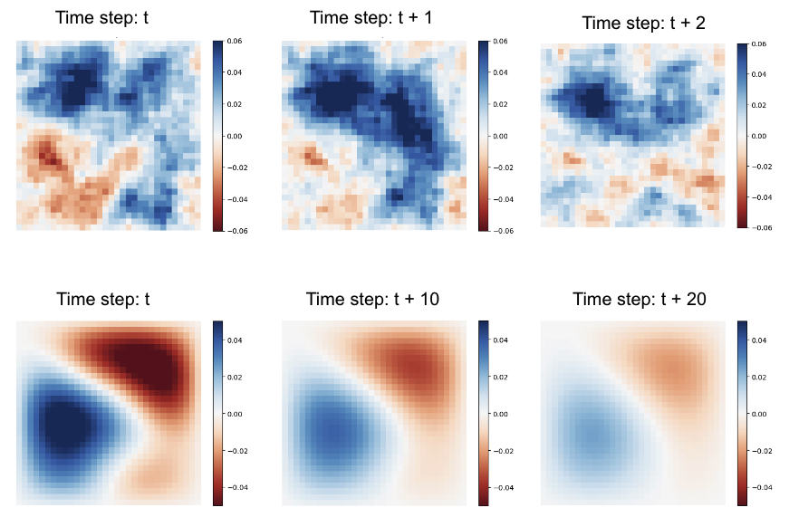
Figure 2: Poisson-AR(1) (top) and 2D Convection-diffusion (bottom) state variables of size $64\times 64$ at three different time steps, which are chosen such that $t$ is sufficiently large for the processes to be in steady state and that the sampling times are adjusted to the temporal dynamics of each process. Here, models parameters used for simulations are: $a=-0.5$ for Poisson-AR, $\theta=0.05$ and $\epsilon=0.01$ for convection-diffusion process; the driving noise is generated from white Gaussian with $\sigma_{w}=0.1$ in both cases.

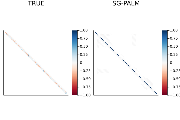
(a) Poisson-AR inverse covariance structure (left) and the estimate obtained by SG-PALM (right).

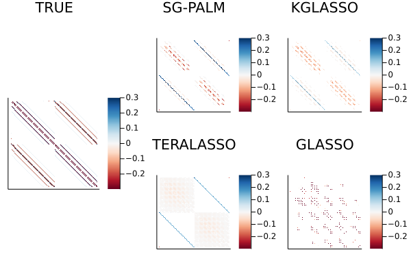
(b) Zoomed-in (middle $128$ rows and columns) Poisson-AR inverse covariance structure (left) and the estimate obtained by SG-PALM, KGlasso, Glasso, TeraLasso (right, clockwise).

Figure 3: Visualizations of the inverse covariance structures for Poisson-AR(1) dynamics and its estimates. Here, white entries indicate zeros in the inverse covariance matrices. The zoomed-in plots show two temporal blocks (each of size $64\times 64$) of spatial inverse correlation structures with the diagonal elements removed for clearer visualization. SG-PALM and the associated Sylvester graphical model produce the richest structures.

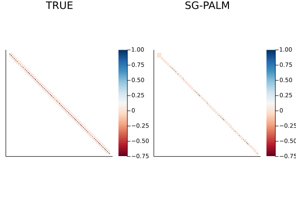
(a) Convection-diffusion inverse covariance structure (left) and the estimate obtained by SG-PALM (right).

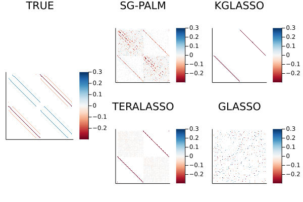
(b) Zoomed-in (middle $128$ rows and columns) convection-diffusion inverse covariance structure (left) and the estimate obtained by SG-PALM, KGlasso, Glasso, TeraLasso (right, clockwise).

Figure 4: Visualizations of the inverse covariance structures for the Convection-Diffusion dynamics and its estimates. Here, white entries indicate zeros in the inverse covariance matrices. The zoomed-in plots show two temporal blocks (each of size $64\times 64$) of spatial inverse correlation structures with the diagonal elements removed for clearer visualization. SG-PALM and the associated Sylvester graphical model produce the richest structures.

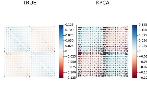
(a) Poisson-AR covariance structure (left) and the estimate obtained by KPCA (right).

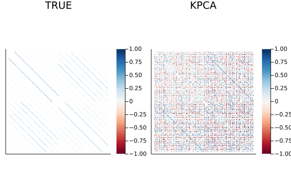
(b) Convection-Diffusion covariance structure (left) and the estimate obtained by KPCA (right).

Figure 5: Visualizations of the middle $128$ rows and columns of the covariance structures for Poisson-AR(1) and Convection-Diffusion dynamics and their estimates, which show two temporal blocks of spatial correlation structures, each of size $64\times 64$, with the diagonal elements removed for clearer visualization of the pattern. Here, white entries indicate zeros in the covariance matrices. Since the covariances are not sparse in general, all matrices are thresholded for clearer inspections of patterns.

Table 3: Comparisons of performances measured by $\log(\|\widehat{{\bm{\Sigma}}}-{\bm{\Sigma}}\|_{F}\text{\textbackslash}\|{\bm{\Sigma}}\|_{F})$ for KPCA as well as $\log(\|\widehat{{\bm{\Omega}}}-{\bm{\Omega}}\|_{F}\text{\textbackslash}\|{\bm{\Omega}}\|_{F})$ and the Mathews Correlation Coefficient (MCC) for SG-PALM, Tlasso, TeraLasso, Glasso. The MCC is a measure of the quality of sparsity recovery considered as a binary classification problem, where $\pm 1$ indicates perfect agreement or disagreement between the truth and the estimation. Here the Frobenius norm errors are included in the first row under each generating type while the MCCs are in the second row. Note that the best performers under each type/criteria are highlighted.

Type	Metric	SG-PALM	KGlasso	TeraLasso	Glasso	KPCA
P-AR	Fnorm	$\mathbf{-0.2622}$	$1.1777$	$0.6312$	$0.9775$	$0.3289$
	MCC	$\mathbf{0.4300}$	$0.3395$	$0.2061$	$0.0560$	N/A
C-D	Fnorm	$\mathbf{-0.0420}$	$1.4919$	$-0.0208$	$2.2041$	$0.0642$
	MCC	$\mathbf{0.2122}$	$0.1884$	$0.2018$	$0.0349$	N/A

Computational efficiencies of the various covariance/precision estimation algorithms are also vitally important in practice to facilitate real-time tracking of physical systems. Table 4 shows the runtime of different covariance and inverse covariance estimation algorithms for the synthetic experiments. It shows that by recognizing and exploiting multiway structures in the data, sparse multiway inverse covariance estimation methods, TeraLasso, Tlasso, and SG-PALM significantly reduce the runtime complexity of Glasso that ignores such special multiway structures. Remark that KPCA runs considerably slower than other methods as it involves expensive singular value decomposition of a large-dimensional re-arranged sample covariance matrix of the data.

Table 4: Average runtime and its standard error (in seconds) of estimating spatio-temporal (inverse) covariance matrices of size $d\times 50$, where $d$ is varying, using various algorithms. Comparisons under various problem sizes (i.e., different $d$ and $N$) are shown. Note the sparse multiway precision models (SG-PALM, KGlasso, TeraLasso) are comparably fast and are all faster than Glasso (for large problems) and KPCA.

$d$	$N$	Glasso	SG-PALM	TeraLasso	KGlasso	KronPCA
		sec	sec	sec	sec	sec
$8^{2}$	$25$	$0.40(0.20)$	$0.46(0.15)$	$0.15(0.35)$	$0.65(0.11)$	$37.22(0.20)$
	$50$	$0.48(0.21)$	$0.47(0.08)$	$0.22(0.50)$	$0.70(0.10)$	$38.22(0.55)$
	$100$	$0.76(0.05)$	$0.44(0.13)$	$0.26(0.28)$	$0.69(0.30)$	$39.09(1.05)$
$16^{2}$	$25$	$6.43(1.45)$	$3.37(1.09)$	$5.38(0.58)$	$5.14(1.99)$	$495.47(2.69)$
	$50$	$9.12(0.98)$	$3.27(1.81)$	$4.62(1.98)$	$3.39(2.00)$	$516.64(2.19)$
	$100$	$11.84(2.01)$	$4.85(1.10)$	$6.71(0.72)$	$5.67(0.57)$	$498.04(4.01)$

4.3 Application to Predicting Evolution of Solar Active Regions

Solar active regions are temporary centers of strong and complex magnetic field on the sun, the principal source of violent eruptions such as solar flares [86]. While weak flares of, for example, B-class, have only limited terrestrial effect, strong flares of M- and X-class can produce tremendous amount of electromagnetic radiation, causing disturbance or damage to satellites, power grids, and communication systems. Therefore, it would be great value to be able to predict how active regions evolve before the onset of solar flares.

Although there are numerous studies that use active region images or physical parameters to predict flare activities [50, 14, 41, 93, 77], fewer studies have attempted to predict the complicated preflare evolution of active regions without physical modeling [4]. In this section, to demonstrate the application of the tensor graphical models, we use multiwavelength active region observations to predict the evolution of two types of active regions that lead to either a weak (B-class) flare or a strong (M- or X-class) flare .

We construct a multiwavelength active region video dataset from the curated dataset generated by Galvez et al. [27]. The video data are taken in four wavelengths (94Å, 131Å, 171Å, and 193Å) by the Atmospheric Imaging Assembly [AIA, 51] aboard the Solar Dynamics Observatory (SDO) satellite. Each video is a 24-hour image sequence of an active region at 1-hour cadence before a strong (M- or X-class) or a weak (B-class) flare occurs in the region. We spatially interpolate the videos so that each video is represented as a $d_{1}\times d_{2}\times d_{3}\times d_{4}$ tensor, where $d_{1}=13$ denotes the number of frames in the video, $d_{2}=50$ denotes the height of the frames after interpolation, $d_{3}=100$ denotes the width of the frames after interpolation, and $d_{4}=4$ represents the number of different channels/wavelength at which the images are recorded. To prevent information leakage, we chronologically split the active region videos into a training set (year 2011 to 2014) and a test set (year 2011 to 2014). In the training set, there are 186 active region videos that lead to a B-class flare and 48 active region videos that lead to a M/X-class flare. In the test set, the sample sizes are 93 and 24 for the B-class and the M/X-class, respectively.

To perform active region prediction, we first fit the tensor graphical models on the training set to estimate the covariance or prediction matrices for each of the two types of active region videos, and then we use the best linear predictor to predict the last frame from all previous frames for videos in the test set. The forward linear predictor is constructed in a multi-output least squares regression setting as

$$\widehat{\mathbf{y}}_{t}=-\mathbf{\Omega}_{2,2}^{-1}\mathbf{\Omega}_{2,1}\mathbf{y}_{t-1:t-(p-1)}$$ (18)

when the precision estimate is available. Here, $t=d_{1}$ for predicting the last frame of a video. For notational convenience, let $p=d_{1}$ and $q=d_{2}d_{3}d_{4}$, then $\mathbf{y}_{t-1:t-(p-1)}=\mathbf{y}_{p-1:1}\in\mathbb{R}^{(p-1)q}$ is the stacked set of pixel values from the previous $p-1$ time instances and $\mathbf{\Omega}_{2,1}\in\mathbb{R}^{q\times(p-1)q}$ and $\mathbf{\Omega}_{2,2}\in\mathbb{R}^{q\times q}$ are submatrices of the $pq\times pq$ estimated precision matrix:

$$\widehat{\mathbf{\Omega}}=\begin{pmatrix}\mathbf{\Omega}_{1,1}&\mathbf{\Omega}_{1,2}\\ \mathbf{\Omega}_{2,1}&\mathbf{\Omega}_{2,2}\end{pmatrix}.$$

The tensor graphical models to be evaluated are SG-PALM (Section 3.5), Tlasso (Section 3.4), and TeraLasso (Section 3.3), with regularization parameters chosen by optimizating the prediction NRMSE (i.e., the root mean squared error normalized by the difference between maximum and minimum pixels) on the training set over a range of $\lambda$ values guided by the convergence rates presented in Table 2. In particular, the SG-PALM estimator was implemented using a regularization parameter $\lambda_{N}=C_{1}\sqrt{\frac{\min(d_{k})\log(d)}{N}}$ for all $k$ with the constant $C_{1}$ chosen by optimizing the prediction NRMSE on the training set over a range of $\lambda$ values parameterized by $C_{1}$. The TeraLasso estimator and the Tlasso estimator were implemented using $\lambda_{N,k}=C_{2}\sqrt{\frac{\log(d)}{N\prod_{i\neq k}d_{i}}}$ and $\lambda_{N,k}=C_{3}\sqrt{\frac{\log(d_{k})}{Nd}}$ for $k=1,2,3$, respectively, with $C_{2},C_{3}$ optimized in a similar manner. Also considered is a baseline estimator, referred to as IndLasso, obtained by applying independent and separate $\ell_{1}$-penalized regressions to each pixel in $\mathbf{y}_{t}$. Each sparse regression in the IndLasso estimator was implemented and tuned independently with regularization parameters chosen in a similar manner. Note that we did not include Glasso and KPCA (Section 3.2) in the comparison due to their prohibitively expensive runtime complexity for large multiway data.

Table 5 shows the NRMSE over the testing samples for the forecasts based on SG-PALM, Tlasso, TeraLasso, and IndLasso. We observe that SG-PALM outperforms all three other methods, indicated by the lowest NRMSEs on the test set. Figure 6 depicts examples of predicted images, comparing with the ground truth. The SG-PALM estimates produced most realistic image predictions that capture the spatially varying structures and closely approximate the pixel values (i.e., maintaining contrast ratios). The latter is important as the flares are being classified into weak (B-class) and strong (M/X-class) categories based on the brightness of the images, and stronger flares are more likely to lead to catastrophic events, such as those that can lead to damaging terrestrial perturbations and health of astronauts.

Predicted examples

AR B

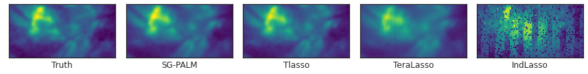
AR B

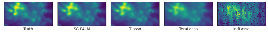
AR M/X

AR M/X

Figure 6: Examples of one-hour ahead prediction of the first two AIA channels of last frames of $13$-frame videos, leading to B- (first two rows) and M/X-class (last two rows) flares, produced by the SG-PALM, Tlasso, TeraLasso, IndLasso algorithms, comparing to the ground truth image (far left column). The column ordering from left to right is in the order of increasing normalized mean squared error (NMSE) - see Table 5. Note that in general linear forward predictors tend to underestimate the contrast ratio of the images. The proposed SG-PALM produced the best-quality images in terms of both the spatial structures and contrast ratios. This figure is excerpted from Wang and Hero [90] (cf. Figure 3 in the reference).

Table 5: Comparison of the SG-PALM, Tlasso, TeraLasso, IndLasso performances measured by NRMSE in predicting the last frame of $13$-frame video sequences leading to B- and M/X-class solar flares. The NRMSEs are computed by averaging across testing samples and AIA channels for each pixel. SG-PALM achieves the best overall NRMSEs across pixels. B flares are generally easier to predict due to both a larger number of samples in the training set and typically smoother transitions from frame to frame within a video.

Flare Type	SG-PALM	Tlasso	TeraLasso	IndLasso
	NRMSE	NRMSE	NRMSE	NRMSE
B	$0.0379$	$0.0386$	$0.0579$	$0.1628$
M/X	$0.0620$	$0.0790$	$0.0913$	$0.1172$

5 Conclusion and discussion

Physical interpretability.

While the Kronecker products expansion used in KPCA captures dense structures in the covariance matrix of data generated from more complex spatio-temporal physical processes, it lacks physical interpretability. In contrast to the case of Sylvester graphical model and Poisson-AR(1) processes, it is not obvious whether the sum of Kronecker products structure corresponds to any true physical models. Recent work in quantum informatics [15] has demonstrated a link between estimation of the density matrix for entangled quantum states and the structured tensor approximation via $\sum_{i=1}^{r}\mathbf{A}_{i}\otimes\mathbf{B}_{i}$. Further characterizing and extending these connections to other classes of discretized PDEs is an interesting future direction. Furthermore, in both the Poisson-AR(1) and convection-diffusion examples, a mixed Kronecker sum and Kronecker product structure emerges that can be related to the state covariance of a dynamical system.

Heavy-tailed multiway covariance/precision models.

Most existing work on multiway covariance and inverse covariance models focus on modeling Gaussian variables. It would be interesting to explore whether the pseudo-likelihood framework we adopted for SyGlasso and SG-PALM can be extended to non-Gaussian heavy-tailed models, e.g., using copula’s or elliptically contoured distributions. This could have important practical applications, in particular to solar flare and active region prediction problems presented in Section 4.3. The images that characterize the active regions generally include a small number of pixels of extreme high-intensity. These pixels might not be captured by a Gaussian-like distribution. Recently, there have been advances [94, 44] in covariance estimation for heavy-tailed, non-Gaussian vector-variate data. Multiway (inverse) covariance estimation is an open problem.

Kronecker-structured autoencoders.

Low-rank covariance models have close connections with variational autoencoders (VAEs). Dai et al. [17] studied the relationship between (robust) PCA and VAEs. Since the Kronecker product for matrices is a generalization of the outer product for vectors, KPCA can be considered as a generalization of a the low-rank approximation method of PCA. It is thus natural to exploit similar relationships between KPCA and VAEs. In this case VAE may be considered as a nonlinear/non-Gaussian extension to KPCA for low separation rank covariance models. Additionally, recent advances in efficient training of the VAE-type neural network architecture (e.g., using stochastic gradient descent) could improve the computational complexity of KPCA that is currently limited by an expensive singular value decomposition [84, 31].

Computational complexity.

Estimating the Kronecker product model is generally hard due to: (i) tensor factorization is NP-hard [35] when $K\geq 3$; and (ii) the optimization objective is nonconvex. The NP-hardness implies computational intractability for large scale problems in the worst case. However, this does not necessarily preclude the existence of tractable solutions for most cases. Specifically, it is believed that the model can be estimated within polynomial time when the signal-to-noise ratio (SNR) is sufficiently high, but only when it is significantly higher than the information-theoretical threshold for model identifiability [72, 37]. While such studies have been completed for some important problems e,g, the statistical-computational gap [10, 103] and the optimization landscape [28], an analogous framework for Kronecker covariance remains to be developed.

While Kronecker sum models do not suffer from the nonconvexity of the Kronecker product model, scalable estimation methods that apply to very large covariance and precision matrices remains computationally challenging. Therefore, it would be worthwhile to develop improvements for the Kronecker sum that mirror the successes in related problems, e.g., introducing more amenable surrogate objectives[6, 45].

Software.

A software package called TensorGraphicalModels [92] has been developed to accompany this review article. Detailed code and instructions for reproducing the numerical results presented in this article (and beyond) are provided in the reference. The software provides a suite of tools in Julia, which was designed specifically for numerical and scientific computing and has recently become popular for large-scale scientific simulation and modeling, such as those conducted by climate scientists [68].

References

- Akdemir and Gupta [2011] {barticle}[author] \bauthor\bsnmAkdemir, \bfnmDeniz\binitsD. and \bauthor\bsnmGupta, \bfnmArjun K\binitsA. K. (\byear2011). \btitleArray Variate Random Variables with Multiway Kronecker Delta Covariance Matrix Structure. \bjournalJournal of algebraic statistics \bvolume2. \endbibitem
- Allen and Tibshirani [2010] {barticle}[author] \bauthor\bsnmAllen, \bfnmGenevera I\binitsG. I. and \bauthor\bsnmTibshirani, \bfnmRobert\binitsR. (\byear2010). \btitleTransposable regularized covariance models with an application to missing data imputation. \bjournalThe Annals of Applied Statistics \bvolume4 \bpages764. \endbibitem
- Allen and Tibshirani [2012] {barticle}[author] \bauthor\bsnmAllen, \bfnmGenevera I\binitsG. I. and \bauthor\bsnmTibshirani, \bfnmRobert\binitsR. (\byear2012). \btitleInference with transposable data: modelling the effects of row and column correlations. \bjournalJournal of the Royal Statistical Society: Series B (Statistical Methodology) \bvolume74 \bpages721–743. \endbibitem
- Bai et al. [2021] {barticle}[author] \bauthor\bsnmBai, \bfnmLiang\binitsL., \bauthor\bsnmBi, \bfnmYi\binitsY., \bauthor\bsnmYang, \bfnmBo\binitsB., \bauthor\bsnmHong, \bfnmJun-Chao\binitsJ.-C., \bauthor\bsnmXu, \bfnmZhe\binitsZ., \bauthor\bsnmShang, \bfnmZhen-Hong\binitsZ.-H., \bauthor\bsnmLiu, \bfnmHui\binitsH., \bauthor\bsnmJi, \bfnmHai-Sheng\binitsH.-S. and \bauthor\bsnmJi, \bfnmKai-Fan\binitsK.-F. (\byear2021). \btitlePredicting the evolution of photospheric magnetic field in solar active regions using deep learning. \bjournalResearch in Astronomy and Astrophysics \bvolume21 \bpages113. \endbibitem
- Banerjee, El Ghaoui and d’Aspremont [2008] {barticle}[author] \bauthor\bsnmBanerjee, \bfnmOnureena\binitsO., \bauthor\bsnmEl Ghaoui, \bfnmLaurent\binitsL. and \bauthor\bsnmd’Aspremont, \bfnmAlexandre\binitsA. (\byear2008). \btitleModel selection through sparse maximum likelihood estimation for multivariate Gaussian or binary data. \bjournalThe Journal of Machine Learning Research \bvolume9 \bpages485–516. \endbibitem
- Besag [1977] {barticle}[author] \bauthor\bsnmBesag, \bfnmJulian\binitsJ. (\byear1977). \btitleEfficiency of pseudolikelihood estimation for simple Gaussian fields. \bjournalBiometrika \bpages616–618. \endbibitem
- Bijma, De Munck and Heethaar [2005] {barticle}[author] \bauthor\bsnmBijma, \bfnmFetsje\binitsF., \bauthor\bsnmDe Munck, \bfnmJan C\binitsJ. C. and \bauthor\bsnmHeethaar, \bfnmRob M\binitsR. M. (\byear2005). \btitleThe spatiotemporal MEG covariance matrix modeled as a sum of Kronecker products. \bjournalNeuroImage \bvolume27 \bpages402–415. \endbibitem
- Box et al. [2015] {bbook}[author] \bauthor\bsnmBox, \bfnmGeorge EP\binitsG. E., \bauthor\bsnmJenkins, \bfnmGwilym M\binitsG. M., \bauthor\bsnmReinsel, \bfnmGregory C\binitsG. C. and \bauthor\bsnmLjung, \bfnmGreta M\binitsG. M. (\byear2015). \btitleTime series analysis: forecasting and control. \bpublisherJohn Wiley & Sons. \endbibitem
- Candès et al. [2011] {barticle}[author] \bauthor\bsnmCandès, \bfnmEmmanuel J\binitsE. J., \bauthor\bsnmLi, \bfnmXiaodong\binitsX., \bauthor\bsnmMa, \bfnmYi\binitsY. and \bauthor\bsnmWright, \bfnmJohn\binitsJ. (\byear2011). \btitleRobust principal component analysis? \bjournalJournal of the ACM (JACM) \bvolume58 \bpages1–37. \endbibitem
- Chandrasekaran and Jordan [2013] {barticle}[author] \bauthor\bsnmChandrasekaran, \bfnmVenkat\binitsV. and \bauthor\bsnmJordan, \bfnmMichael I\binitsM. I. (\byear2013). \btitleComputational and statistical tradeoffs via convex relaxation. \bjournalProceedings of the National Academy of Sciences \bvolume110 \bpagesE1181–E1190. \endbibitem
- Chandrasekaran et al. [2011] {barticle}[author] \bauthor\bsnmChandrasekaran, \bfnmVenkat\binitsV., \bauthor\bsnmSanghavi, \bfnmSujay\binitsS., \bauthor\bsnmParrilo, \bfnmPablo A\binitsP. A. and \bauthor\bsnmWillsky, \bfnmAlan S\binitsA. S. (\byear2011). \btitleRank-sparsity incoherence for matrix decomposition. \bjournalSIAM Journal on Optimization \bvolume21 \bpages572–596. \endbibitem
- Chandrasekhar [1943] {barticle}[author] \bauthor\bsnmChandrasekhar, \bfnmSubrahmanyan\binitsS. (\byear1943). \btitleStochastic problems in physics and astronomy. \bjournalReviews of modern physics \bvolume15 \bpages1. \endbibitem
- Chen, Wiesel and Hero [2011] {barticle}[author] \bauthor\bsnmChen, \bfnmYilun\binitsY., \bauthor\bsnmWiesel, \bfnmAmi\binitsA. and \bauthor\bsnmHero, \bfnmAlfred O\binitsA. O. (\byear2011). \btitleRobust shrinkage estimation of high-dimensional covariance matrices. \bjournalIEEE Transactions on Signal Processing \bvolume59 \bpages4097–4107. \endbibitem
- Chen et al. [2019] {barticle}[author] \bauthor\bsnmChen, \bfnmYang\binitsY., \bauthor\bsnmManchester, \bfnmWard B\binitsW. B., \bauthor\bsnmHero, \bfnmAlfred O\binitsA. O., \bauthor\bsnmToth, \bfnmGabor\binitsG., \bauthor\bsnmDuFumier, \bfnmBenoit\binitsB., \bauthor\bsnmZhou, \bfnmTian\binitsT., \bauthor\bsnmWang, \bfnmXiantong\binitsX., \bauthor\bsnmZhu, \bfnmHaonan\binitsH., \bauthor\bsnmSun, \bfnmZeyu\binitsZ. and \bauthor\bsnmGombosi, \bfnmTamas I\binitsT. I. (\byear2019). \btitleIdentifying solar flare precursors using time series of SDO/HMI images and SHARP parameters. \bjournalSpace Weather \bvolume17 \bpages1404–1426. \endbibitem
- Chu and Lin [2021] {barticle}[author] \bauthor\bsnmChu, \bfnmMoody T\binitsM. T. and \bauthor\bsnmLin, \bfnmMatthew M\binitsM. M. (\byear2021). \btitleNonlinear Power-Like and SVD-Like Iterative Schemes with Applications to Entangled Bipartite Rank-1 Approximation. \bjournalSIAM Journal on Scientific Computing \bvolume0 \bpagesS448–S474. \endbibitem
- Cressie [2015] {bbook}[author] \bauthor\bsnmCressie, \bfnmNoel\binitsN. (\byear2015). \btitleStatistics for spatial data. \bpublisherJohn Wiley & Sons. \endbibitem
- Dai et al. [2018] {barticle}[author] \bauthor\bsnmDai, \bfnmBin\binitsB., \bauthor\bsnmWang, \bfnmYu\binitsY., \bauthor\bsnmAston, \bfnmJohn\binitsJ., \bauthor\bsnmHua, \bfnmGang\binitsG. and \bauthor\bsnmWipf, \bfnmDavid\binitsD. (\byear2018). \btitleConnections with robust PCA and the role of emergent sparsity in variational autoencoder models. \bjournalThe Journal of Machine Learning Research \bvolume19 \bpages1573–1614. \endbibitem
- Dantas, Cohen and Gribonval [2019] {binproceedings}[author] \bauthor\bsnmDantas, \bfnmCássio F\binitsC. F., \bauthor\bsnmCohen, \bfnmJérémy E\binitsJ. E. and \bauthor\bsnmGribonval, \bfnmRémi\binitsR. (\byear2019). \btitleLearning tensor-structured dictionaries with application to hyperspectral image denoising. In \bbooktitle2019 27th European Signal Processing Conference (EUSIPCO) \bpages1–5. \bpublisherIEEE. \endbibitem
- Dawid [1981] {barticle}[author] \bauthor\bsnmDawid, \bfnmA Philip\binitsA. P. (\byear1981). \btitleSome matrix-variate distribution theory: notational considerations and a Bayesian application. \bjournalBiometrika \bvolume68 \bpages265–274. \endbibitem
- Deng, Tang and Qu [2021] {barticle}[author] \bauthor\bsnmDeng, \bfnmYujia\binitsY., \bauthor\bsnmTang, \bfnmXiwei\binitsX. and \bauthor\bsnmQu, \bfnmAnnie\binitsA. (\byear2021). \btitleCorrelation Tensor Decomposition and Its Application in Spatial Imaging Data. \bjournalJournal of the American Statistical Association \bvolumejust-accepted \bpages1–35. \endbibitem
- Du et al. [2017] {barticle}[author] \bauthor\bsnmDu, \bfnmJiewen\binitsJ., \bauthor\bsnmYan, \bfnmXin\binitsX., \bauthor\bsnmLiu, \bfnmZhihong\binitsZ., \bauthor\bsnmCui, \bfnmLu\binitsL., \bauthor\bsnmDing, \bfnmPeng\binitsP., \bauthor\bsnmTan, \bfnmXiaoqing\binitsX., \bauthor\bsnmLi, \bfnmXiuming\binitsX., \bauthor\bsnmZhou, \bfnmHuihao\binitsH., \bauthor\bsnmGu, \bfnmQiong\binitsQ. and \bauthor\bsnmXu, \bfnmJun\binitsJ. (\byear2017). \btitlecBinderDB: a covalent binding agent database. \bjournalBioinformatics \bvolume33 \bpages1258–1260. \endbibitem
- Dutilleul [1999] {barticle}[author] \bauthor\bsnmDutilleul, \bfnmPierre\binitsP. (\byear1999). \btitleThe MLE algorithm for the matrix normal distribution. \bjournalJournal of statistical computation and simulation \bvolume64 \bpages105–123. \endbibitem
- Evensen [1994] {barticle}[author] \bauthor\bsnmEvensen, \bfnmGeir\binitsG. (\byear1994). \btitleSequential data assimilation with a nonlinear quasi-geostrophic model using Monte Carlo methods to forecast error statistics. \bjournalJournal of Geophysical Research: Oceans \bvolume99 \bpages10143–10162. \endbibitem
- Friedman, Hastie and Tibshirani [2008] {barticle}[author] \bauthor\bsnmFriedman, \bfnmJerome\binitsJ., \bauthor\bsnmHastie, \bfnmTrevor\binitsT. and \bauthor\bsnmTibshirani, \bfnmRobert\binitsR. (\byear2008). \btitleSparse inverse covariance estimation with the graphical lasso. \bjournalBiostatistics \bvolume9 \bpages432–441. \endbibitem
- Fu and Huang [2008] {barticle}[author] \bauthor\bsnmFu, \bfnmYun\binitsY. and \bauthor\bsnmHuang, \bfnmThomas S\binitsT. S. (\byear2008). \btitleImage classification using correlation tensor analysis. \bjournalIEEE Transactions on Image Processing \bvolume17 \bpages226–234. \endbibitem
- Galecki [1994] {barticle}[author] \bauthor\bsnmGalecki, \bfnmAndrzej T\binitsA. T. (\byear1994). \btitleGeneral class of covariance structures for two or more repeated factors in longitudinal data analysis. \bjournalCommunications in Statistics-Theory and Methods \bvolume23 \bpages3105–3119. \endbibitem
- Galvez et al. [2019] {barticle}[author] \bauthor\bsnmGalvez, \bfnmRichard\binitsR., \bauthor\bsnmFouhey, \bfnmDavid F\binitsD. F., \bauthor\bsnmJin, \bfnmMeng\binitsM., \bauthor\bsnmSzenicer, \bfnmAlexandre\binitsA., \bauthor\bsnmMuñoz-Jaramillo, \bfnmAndrés\binitsA., \bauthor\bsnmCheung, \bfnmMark CM\binitsM. C., \bauthor\bsnmWright, \bfnmPaul J\binitsP. J., \bauthor\bsnmBobra, \bfnmMonica G\binitsM. G., \bauthor\bsnmLiu, \bfnmYang\binitsY., \bauthor\bsnmMason, \bfnmJames\binitsJ. \betalet al. (\byear2019). \btitleA machine-learning data set prepared from the NASA solar dynamics observatory mission. \bjournalThe Astrophysical Journal Supplement Series \bvolume242 \bpages7. \endbibitem
- Ge and Ma [2020] {barticle}[author] \bauthor\bsnmGe, \bfnmRong\binitsR. and \bauthor\bsnmMa, \bfnmTengyu\binitsT. (\byear2020). \btitleOn the optimization landscape of tensor decompositions. \bjournalMathematical Programming \bpages1–47. \endbibitem
- Grasedyck [2004] {barticle}[author] \bauthor\bsnmGrasedyck, \bfnmLars\binitsL. (\byear2004). \btitleExistence and computation of low Kronecker-rank approximations for large linear systems of tensor product structure. \bjournalComputing \bvolume72 \bpages247–265. \endbibitem
- Greenewald and Hero [2014] {binproceedings}[author] \bauthor\bsnmGreenewald, \bfnmKristjan H\binitsK. H. and \bauthor\bsnmHero, \bfnmAlfred O\binitsA. O. (\byear2014). \btitleKronecker PCA based spatio-temporal modeling of video for dismount classification. In \bbooktitleAlgorithms for Synthetic Aperture Radar Imagery XXI \bvolume9093 \bpages90930V. \bpublisherInternational Society for Optics and Photonics. \endbibitem
- Greenewald and Hero [2015] {barticle}[author] \bauthor\bsnmGreenewald, \bfnmKristjan\binitsK. and \bauthor\bsnmHero, \bfnmAlfred O\binitsA. O. (\byear2015). \btitleRobust kronecker product PCA for spatio-temporal covariance estimation. \bjournalIEEE Transactions on Signal Processing \bvolume63 \bpages6368–6378. \endbibitem
- Greenewald, Zelnio and Hero [2016] {barticle}[author] \bauthor\bsnmGreenewald, \bfnmKristjan\binitsK., \bauthor\bsnmZelnio, \bfnmEdmund\binitsE. and \bauthor\bsnmHero, \bfnmAlfred Hero\binitsA. H. (\byear2016). \btitleRobust SAR STAP via Kronecker decomposition. \bjournalIEEE Transactions on Aerospace and Electronic Systems \bvolume52 \bpages2612–2625. \endbibitem
- Greenewald, Zhou and Hero [2019] {barticle}[author] \bauthor\bsnmGreenewald, \bfnmKristjan\binitsK., \bauthor\bsnmZhou, \bfnmShuheng\binitsS. and \bauthor\bsnmHero, \bfnmAlfred\binitsA. (\byear2019). \btitleTensor graphical lasso (TeraLasso). \bjournalJournal of the Royal Statistical Society: Series B (Statistical Methodology) \bvolume81 \bpages901–931. \endbibitem
- Hao et al. [2021] {barticle}[author] \bauthor\bsnmHao, \bfnmBotao\binitsB., \bauthor\bsnmWang, \bfnmBoxiang\binitsB., \bauthor\bsnmWang, \bfnmPengyuan\binitsP., \bauthor\bsnmZhang, \bfnmJingfei\binitsJ., \bauthor\bsnmYang, \bfnmJian\binitsJ. and \bauthor\bsnmSun, \bfnmWill Wei\binitsW. W. (\byear2021). \btitleSparse tensor additive regression. \bjournalJournal of Machine Learning Research \bvolume22 \bpages1–43. \endbibitem
- Hillar and Lim [2013] {barticle}[author] \bauthor\bsnmHillar, \bfnmChristopher J\binitsC. J. and \bauthor\bsnmLim, \bfnmLek-Heng\binitsL.-H. (\byear2013). \btitleMost tensor problems are NP-hard. \bjournalJournal of the ACM (JACM) \bvolume60 \bpages1–39. \endbibitem
- Hoff [2011] {barticle}[author] \bauthor\bsnmHoff, \bfnmPeter D\binitsP. D. (\byear2011). \btitleSeparable covariance arrays via the Tucker product, with applications to multivariate relational data. \bjournalBayesian Analysis \bvolume6 \bpages179–196. \endbibitem
- Hopkins, Shi and Steurer [2015] {binproceedings}[author] \bauthor\bsnmHopkins, \bfnmSamuel B\binitsS. B., \bauthor\bsnmShi, \bfnmJonathan\binitsJ. and \bauthor\bsnmSteurer, \bfnmDavid\binitsD. (\byear2015). \btitleTensor principal component analysis via sum-of-square proofs. In \bbooktitleConference on Learning Theory \bpages956–1006. \bpublisherPMLR. \endbibitem
- Hori et al. [2016] {barticle}[author] \bauthor\bsnmHori, \bfnmTomoaki\binitsT., \bauthor\bsnmMontcho, \bfnmDavid\binitsD., \bauthor\bsnmAgbangla, \bfnmClement\binitsC., \bauthor\bsnmEbana, \bfnmKaworu\binitsK., \bauthor\bsnmFutakuchi, \bfnmKoichi\binitsK. and \bauthor\bsnmIwata, \bfnmHiroyoshi\binitsH. (\byear2016). \btitleMulti-task Gaussian process for imputing missing data in multi-trait and multi-environment trials. \bjournalTheoretical and Applied Genetics \bvolume129 \bpages2101–2115. \endbibitem
- Hou, Lawrence and Hero [2021] {barticle}[author] \bauthor\bsnmHou, \bfnmElizabeth\binitsE., \bauthor\bsnmLawrence, \bfnmEarl\binitsE. and \bauthor\bsnmHero, \bfnmAlfred O\binitsA. O. (\byear2021). \btitlePenalized ensemble Kalman filters for high dimensional non-linear systems. \bjournalPloS one \bvolume16 \bpagese0248046. \endbibitem
- Jiang, Bigot and Maabout [2021] {barticle}[author] \bauthor\bsnmJiang, \bfnmYiye\binitsY., \bauthor\bsnmBigot, \bfnmJérémie\binitsJ. and \bauthor\bsnmMaabout, \bfnmSofian\binitsS. (\byear2021). \btitleOnline Graph Topology Learning from Matrix-valued Time Series. \bjournalarXiv preprint arXiv:2107.08020. \endbibitem
- Jiao et al. [2020] {barticle}[author] \bauthor\bsnmJiao, \bfnmZhenbang\binitsZ., \bauthor\bsnmSun, \bfnmHu\binitsH., \bauthor\bsnmWang, \bfnmXiantong\binitsX., \bauthor\bsnmManchester, \bfnmWard\binitsW., \bauthor\bsnmGombosi, \bfnmTamas\binitsT., \bauthor\bsnmHero, \bfnmAlfred\binitsA. and \bauthor\bsnmChen, \bfnmYang\binitsY. (\byear2020). \btitleSolar flare intensity prediction with machine learning models. \bjournalSpace Weather \bvolume18 \bpagese2020SW002440. \endbibitem
- Jolliffe [1986] {bincollection}[author] \bauthor\bsnmJolliffe, \bfnmIan T\binitsI. T. (\byear1986). \btitlePrincipal components in regression analysis. In \bbooktitlePrincipal component analysis \bpages129–155. \bpublisherSpringer. \endbibitem
- Kalaitzis et al. [2013] {binproceedings}[author] \bauthor\bsnmKalaitzis, \bfnmAlfredo\binitsA., \bauthor\bsnmLafferty, \bfnmJohn\binitsJ., \bauthor\bsnmLawrence, \bfnmNeil D\binitsN. D. and \bauthor\bsnmZhou, \bfnmShuheng\binitsS. (\byear2013). \btitleThe bigraphical lasso. In \bbooktitleInternational Conference on Machine Learning \bpages1229–1237. \bpublisherPMLR. \endbibitem
- Ke et al. [2019] {barticle}[author] \bauthor\bsnmKe, \bfnmYuan\binitsY., \bauthor\bsnmMinsker, \bfnmStanislav\binitsS., \bauthor\bsnmRen, \bfnmZhao\binitsZ., \bauthor\bsnmSun, \bfnmQiang\binitsQ. and \bauthor\bsnmZhou, \bfnmWen-Xin\binitsW.-X. (\byear2019). \btitleUser-friendly covariance estimation for heavy-tailed distributions. \bjournalStatistical Science \bvolume34 \bpages454–471. \endbibitem
- Khare, Oh and Rajaratnam [2015] {barticle}[author] \bauthor\bsnmKhare, \bfnmKshitij\binitsK., \bauthor\bsnmOh, \bfnmSang-Yun\binitsS.-Y. and \bauthor\bsnmRajaratnam, \bfnmBala\binitsB. (\byear2015). \btitleA convex pseudolikelihood framework for high dimensional partial correlation estimation with convergence guarantees. \bjournalJournal of the Royal Statistical Society: Series B: Statistical Methodology \bpages803–825. \endbibitem
- Kolda and Bader [2009] {barticle}[author] \bauthor\bsnmKolda, \bfnmTamara G\binitsT. G. and \bauthor\bsnmBader, \bfnmBrett W\binitsB. W. (\byear2009). \btitleTensor decompositions and applications. \bjournalSIAM review \bvolume51 \bpages455–500. \endbibitem
- Kressner and Tobler [2010] {barticle}[author] \bauthor\bsnmKressner, \bfnmDaniel\binitsD. and \bauthor\bsnmTobler, \bfnmChristine\binitsC. (\byear2010). \btitleKrylov subspace methods for linear systems with tensor product structure. \bjournalSIAM journal on matrix analysis and applications \bvolume31 \bpages1688–1714. \endbibitem
- Landsberg [2011] {bbook}[author] \bauthor\bsnmLandsberg, \bfnmJM\binitsJ. (\byear2011). \btitleTensors: Geometry and Applications: Geometry and Applications \bvolume128. \bpublisherAmerican Mathematical Soc. \endbibitem
- Ledoit and Wolf [2020] {barticle}[author] \bauthor\bsnmLedoit, \bfnmOlivier\binitsO. and \bauthor\bsnmWolf, \bfnmMichael\binitsM. (\byear2020). \btitleThe power of (non-) linear shrinking: A review and guide to covariance matrix estimation. \bjournalJournal of Financial Econometrics. \endbibitem
- Leka and Barnes [2003] {barticle}[author] \bauthor\bsnmLeka, \bfnmKD\binitsK. and \bauthor\bsnmBarnes, \bfnmG\binitsG. (\byear2003). \btitlePhotospheric magnetic field properties of flaring versus flare-quiet active regions. II. Discriminant analysis. \bjournalThe Astrophysical Journal \bvolume595 \bpages1296. \endbibitem
- Lemen et al. [2011] {bincollection}[author] \bauthor\bsnmLemen, \bfnmJames R\binitsJ. R., \bauthor\bsnmAkin, \bfnmDavid J\binitsD. J., \bauthor\bsnmBoerner, \bfnmPaul F\binitsP. F., \bauthor\bsnmChou, \bfnmCatherine\binitsC., \bauthor\bsnmDrake, \bfnmJerry F\binitsJ. F., \bauthor\bsnmDuncan, \bfnmDexter W\binitsD. W., \bauthor\bsnmEdwards, \bfnmChristopher G\binitsC. G., \bauthor\bsnmFriedlaender, \bfnmFrank M\binitsF. M., \bauthor\bsnmHeyman, \bfnmGary F\binitsG. F., \bauthor\bsnmHurlburt, \bfnmNeal E\binitsN. E. \betalet al. (\byear2011). \btitleThe atmospheric imaging assembly (AIA) on the solar dynamics observatory (SDO). In \bbooktitleThe solar dynamics observatory \bpages17–40. \bpublisherSpringer. \endbibitem
- Leng and Pan [2018] {barticle}[author] \bauthor\bsnmLeng, \bfnmChenlei\binitsC. and \bauthor\bsnmPan, \bfnmGuangming\binitsG. (\byear2018). \btitleCovariance estimation via sparse Kronecker structures. \bjournalBernoulli \bvolume24 \bpages3833–3863. \endbibitem
- Li and Zhang [2017] {barticle}[author] \bauthor\bsnmLi, \bfnmLexin\binitsL. and \bauthor\bsnmZhang, \bfnmXin\binitsX. (\byear2017). \btitleParsimonious tensor response regression. \bjournalJournal of the American Statistical Association \bvolume112 \bpages1131–1146. \endbibitem
- Li et al. [2008] {barticle}[author] \bauthor\bsnmLi, \bfnmZhijin\binitsZ., \bauthor\bsnmChao, \bfnmYi\binitsY., \bauthor\bsnmMcWilliams, \bfnmJames C\binitsJ. C. and \bauthor\bsnmIde, \bfnmKayo\binitsK. (\byear2008). \btitleA three-dimensional variational data assimilation scheme for the regional ocean modeling system. \bjournalJournal of Atmospheric and Oceanic Technology \bvolume25 \bpages2074–2090. \endbibitem
- Li et al. [2022] {barticle}[author] \bauthor\bsnmLi, \bfnmSijia\binitsS., \bauthor\bsnmLópez-García, \bfnmMartín\binitsM., \bauthor\bsnmLawrence, \bfnmNeil D\binitsN. D. and \bauthor\bsnmCutillo, \bfnmLuisa\binitsL. (\byear2022). \btitleScalable Bigraphical Lasso: Two-way Sparse Network Inference for Count Data. \bjournalarXiv preprint arXiv:2203.07912. \endbibitem
- Lindgren, Rue and Lindström [2011] {barticle}[author] \bauthor\bsnmLindgren, \bfnmFinn\binitsF., \bauthor\bsnmRue, \bfnmHåvard\binitsH. and \bauthor\bsnmLindström, \bfnmJohan\binitsJ. (\byear2011). \btitleAn explicit link between Gaussian fields and Gaussian Markov random fields: the stochastic partial differential equation approach. \bjournalJournal of the Royal Statistical Society: Series B (Statistical Methodology) \bvolume73 \bpages423–498. \endbibitem
- Liu et al. [2019] {barticle}[author] \bauthor\bsnmLiu, \bfnmGang\binitsG., \bauthor\bsnmTan, \bfnmXiaoqing\binitsX., \bauthor\bsnmDang, \bfnmChao\binitsC., \bauthor\bsnmTan, \bfnmShuangquan\binitsS., \bauthor\bsnmXing, \bfnmShihui\binitsS., \bauthor\bsnmHuang, \bfnmNianwei\binitsN., \bauthor\bsnmPeng, \bfnmKangqiang\binitsK., \bauthor\bsnmXie, \bfnmChuanmiao\binitsC., \bauthor\bsnmTang, \bfnmXiaoying\binitsX. and \bauthor\bsnmZeng, \bfnmJinsheng\binitsJ. (\byear2019). \btitleRegional shape abnormalities in thalamus and verbal memory impairment after subcortical infarction. \bjournalNeurorehabilitation and Neural Repair \bvolume33 \bpages476–485. \endbibitem
- Llosa-Vite and Maitra [2022] {barticle}[author] \bauthor\bsnmLlosa-Vite, \bfnmCarlos\binitsC. and \bauthor\bsnmMaitra, \bfnmRanjan\binitsR. (\byear2022). \btitleReduced-Rank Tensor-on-Tensor Regression and Tensor-variate Analysis of Variance. \bjournalIEEE Transactions on Pattern Analysis and Machine Intelligence \bpages1-1. \bdoi10.1109/TPAMI.2022.3164836 \endbibitem
- Lyu et al. [2019] {barticle}[author] \bauthor\bsnmLyu, \bfnmXiang\binitsX., \bauthor\bsnmSun, \bfnmWill Wei\binitsW. W., \bauthor\bsnmWang, \bfnmZhaoran\binitsZ., \bauthor\bsnmLiu, \bfnmHan\binitsH., \bauthor\bsnmYang, \bfnmJian\binitsJ. and \bauthor\bsnmCheng, \bfnmGuang\binitsG. (\byear2019). \btitleTensor graphical model: Non-convex optimization and statistical inference. \bjournalIEEE transactions on pattern analysis and machine intelligence \bvolume42 \bpages2024–2037. \endbibitem
- Manceur and Dutilleul [2013] {barticle}[author] \bauthor\bsnmManceur, \bfnmAmeur M\binitsA. M. and \bauthor\bsnmDutilleul, \bfnmPierre\binitsP. (\byear2013). \btitleMaximum likelihood estimation for the tensor normal distribution: Algorithm, minimum sample size, and empirical bias and dispersion. \bjournalJournal of Computational and Applied Mathematics \bvolume239 \bpages37–49. \endbibitem
- Mardia and Goodall [1993] {barticle}[author] \bauthor\bsnmMardia, \bfnmKanti V\binitsK. V. and \bauthor\bsnmGoodall, \bfnmColin R\binitsC. R. (\byear1993). \btitleSpatial-temporal analysis of multivariate environmental monitoring data. \bjournalMultivariate environmental statistics \bvolume6 \bpages347–385. \endbibitem
- Matthews [1975] {barticle}[author] \bauthor\bsnmMatthews, \bfnmBrian W\binitsB. W. (\byear1975). \btitleComparison of the predicted and observed secondary structure of T4 phage lysozyme. \bjournalBiochimica et Biophysica Acta (BBA)-Protein Structure \bvolume405 \bpages442–451. \endbibitem
- Meinshausen and Bühlmann [2006] {barticle}[author] \bauthor\bsnmMeinshausen, \bfnmNicolai\binitsN. and \bauthor\bsnmBühlmann, \bfnmPeter\binitsP. (\byear2006). \btitleHigh-dimensional graphs and variable selection with the lasso. \bjournalThe annals of statistics \bvolume34 \bpages1436–1462. \endbibitem
- Min, Mai and Zhang [2022] {barticle}[author] \bauthor\bsnmMin, \bfnmKeqian\binitsK., \bauthor\bsnmMai, \bfnmQing\binitsQ. and \bauthor\bsnmZhang, \bfnmXin\binitsX. (\byear2022). \btitleFast and separable estimation in high-dimensional tensor Gaussian graphical models. \bjournalJournal of Computational and Graphical Statistics \bvolume31 \bpages294–300. \endbibitem
- Mo et al. [2022] {barticle}[author] \bauthor\bsnmMo, \bfnmShentong\binitsS., \bauthor\bsnmXia, \bfnmJingfei\binitsJ., \bauthor\bsnmTan, \bfnmXiaoqing\binitsX. and \bauthor\bsnmRaj, \bfnmBhiksha\binitsB. (\byear2022). \btitlePoint3D: tracking actions as moving points with 3D CNNs. \bjournalarXiv preprint arXiv:2203.10584. \endbibitem
- Molstad and Rothman [2019] {barticle}[author] \bauthor\bsnmMolstad, \bfnmAaron J\binitsA. J. and \bauthor\bsnmRothman, \bfnmAdam J\binitsA. J. (\byear2019). \btitleA penalized likelihood method for classification with matrix-valued predictors. \bjournalJournal of Computational and Graphical Statistics \bvolume28 \bpages11–22. \endbibitem
- Ohlson, Ahmad and Von Rosen [2013] {barticle}[author] \bauthor\bsnmOhlson, \bfnmMartin\binitsM., \bauthor\bsnmAhmad, \bfnmM Rauf\binitsM. R. and \bauthor\bsnmVon Rosen, \bfnmDietrich\binitsD. (\byear2013). \btitleThe multilinear normal distribution: Introduction and some basic properties. \bjournalJournal of Multivariate Analysis \bvolume113 \bpages37–47. \endbibitem
- Perkel [2019] {barticle}[author] \bauthor\bsnmPerkel, \bfnmJeffrey M\binitsJ. M. (\byear2019). \btitleJulia: come for the syntax, stay for the speed. \bjournalNature \bvolume572 \bpages141–143. \endbibitem
- Pourahmadi [2011] {barticle}[author] \bauthor\bsnmPourahmadi, \bfnmMohsen\binitsM. (\byear2011). \btitleCovariance estimation: The GLM and regularization perspectives. \bjournalStatistical Science \bvolume26 \bpages369–387. \endbibitem
- Pouryazdian, Beheshti and Krishnan [2016] {barticle}[author] \bauthor\bsnmPouryazdian, \bfnmSaeed\binitsS., \bauthor\bsnmBeheshti, \bfnmSoosan\binitsS. and \bauthor\bsnmKrishnan, \bfnmSridhar\binitsS. (\byear2016). \btitleCANDECOMP/PARAFAC model order selection based on reconstruction error in the presence of kronecker structured colored noise. \bjournalDigital Signal Processing \bvolume48 \bpages12–26. \endbibitem
- Rabusseau and Kadri [2016] {barticle}[author] \bauthor\bsnmRabusseau, \bfnmGuillaume\binitsG. and \bauthor\bsnmKadri, \bfnmHachem\binitsH. (\byear2016). \btitleLow-rank regression with tensor responses. \bjournalAdvances in Neural Information Processing Systems \bvolume29 \bpages1867–1875. \endbibitem
- Richard and Montanari [2014] {barticle}[author] \bauthor\bsnmRichard, \bfnmEmile\binitsE. and \bauthor\bsnmMontanari, \bfnmAndrea\binitsA. (\byear2014). \btitleA statistical model for tensor PCA. \bjournalAdvances in Neural Information Processing Systems \bvolume27 \bpages2897–2905. \endbibitem
- Roberts [2006] {barticle}[author] \bauthor\bsnmRoberts, \bfnmB\binitsB. (\byear2006). \btitleSlow magnetohydrodynamic waves in the solar atmosphere. \bjournalPhilosophical Transactions of the Royal Society A: Mathematical, Physical and Engineering Sciences \bvolume364 \bpages447–460. \endbibitem
- Stocker [2011] {bbook}[author] \bauthor\bsnmStocker, \bfnmThomas\binitsT. (\byear2011). \btitleIntroduction to climate modelling. \bpublisherSpringer Science & Business Media. \endbibitem
- Strobach [1995] {barticle}[author] \bauthor\bsnmStrobach, \bfnmPeter\binitsP. (\byear1995). \btitleLow-rank detection of multichannel Gaussian signals using block matrix approximation. \bjournalIEEE Transactions on Signal Processing \bvolume43 \bpages233–242. \endbibitem
- [76] {barticle}[author] \bauthor\bsnmSun, \bfnmWill Wei\binitsW. W., \bauthor\bsnmHao, \bfnmBotao\binitsB. and \bauthor\bsnmLi, \bfnmLexin\binitsL. \btitleTensors in Modern Statistical Learning. \endbibitem
- Sun et al. [2021] {barticle}[author] \bauthor\bsnmSun, \bfnmZeyu\binitsZ., \bauthor\bsnmBobra, \bfnmMonica\binitsM., \bauthor\bsnmWang, \bfnmXiantong\binitsX., \bauthor\bsnmWang, \bfnmYu\binitsY., \bauthor\bsnmSun, \bfnmHu\binitsH., \bauthor\bsnmGombosi, \bfnmTamas\binitsT., \bauthor\bsnmChen, \bfnmYang\binitsY. and \bauthor\bsnmHero, \bfnmAlfred\binitsA. (\byear2021). \btitlePredicting Solar Flares using CNN and LSTM on Two Solar Cycles of Active Region Data. \bjournalEarth and Space Science Open Archive \bpages32. \bdoi10.1002/essoar.10508256.1 \endbibitem
- Tan et al. [2018] {binproceedings}[author] \bauthor\bsnmTan, \bfnmXiaoqing\binitsX., \bauthor\bsnmRoss, \bfnmChristopher A\binitsC. A., \bauthor\bsnmMiller, \bfnmMichaeli\binitsM. and \bauthor\bsnmTang, \bfnmXiaoying\binitsX. (\byear2018). \btitleChangepoint analysis of putamen and thalamus subregions in premanifest huntington’s disease. In \bbooktitle2018 IEEE 15th International Symposium on Biomedical Imaging (ISBI 2018) \bpages531–535. \bpublisherIEEE. \endbibitem
- Tan et al. [2022a] {barticle}[author] \bauthor\bsnmTan, \bfnmXiaoqing\binitsX., \bauthor\bsnmQi, \bfnmZhengling\binitsZ., \bauthor\bsnmSeymour, \bfnmChristopher W\binitsC. W. and \bauthor\bsnmTang, \bfnmLu\binitsL. (\byear2022a). \btitleRISE: Robust Individualized Decision Learning with Sensitive Variables. \bjournalarXiv preprint arXiv:2211.06569. \endbibitem
- Tan et al. [2022b] {binproceedings}[author] \bauthor\bsnmTan, \bfnmXiaoqing\binitsX., \bauthor\bsnmAbberbock, \bfnmJudah\binitsJ., \bauthor\bsnmRastogi, \bfnmPriya\binitsP. and \bauthor\bsnmTang, \bfnmGong\binitsG. (\byear2022b). \btitleIdentifying Principal Stratum Causal Effects Conditional on a Post-treatment Intermediate Response. In \bbooktitleConference on Causal Learning and Reasoning \bpages734–753. \bpublisherPMLR. \endbibitem
- Tan et al. [2022c] {barticle}[author] \bauthor\bsnmTan, \bfnmXiaoqing\binitsX., \bauthor\bsnmYang, \bfnmShu\binitsS., \bauthor\bsnmYe, \bfnmWenyu\binitsW., \bauthor\bsnmFaries, \bfnmDouglas E\binitsD. E., \bauthor\bsnmLipkovich, \bfnmIlya\binitsI. and \bauthor\bsnmKadziola, \bfnmZbigniew\binitsZ. (\byear2022c). \btitleWhen Doubly Robust Methods Meet Machine Learning for Estimating Treatment Effects from Real-World Data: A Comparative Study. \bjournalarXiv preprint arXiv:2204.10969. \endbibitem
- Tan et al. [2022d] {binproceedings}[author] \bauthor\bsnmTan, \bfnmXiaoqing\binitsX., \bauthor\bsnmChang, \bfnmChung-Chou H\binitsC.-C. H., \bauthor\bsnmZhou, \bfnmLing\binitsL. and \bauthor\bsnmTang, \bfnmLu\binitsL. (\byear2022d). \btitleA tree-based model averaging approach for personalized treatment effect estimation from heterogeneous data sources. In \bbooktitleInternational Conference on Machine Learning \bpages21013–21036. \bpublisherPMLR. \endbibitem
- Teng and Huang [2009] {barticle}[author] \bauthor\bsnmTeng, \bfnmSiew Leng\binitsS. L. and \bauthor\bsnmHuang, \bfnmHaiyan\binitsH. (\byear2009). \btitleA statistical framework to infer functional gene relationships from biologically interrelated microarray experiments. \bjournalJournal of the American Statistical Association \bvolume104 \bpages465–473. \endbibitem
- Tsiligkaridis and Hero [2013] {barticle}[author] \bauthor\bsnmTsiligkaridis, \bfnmTheodoros\binitsT. and \bauthor\bsnmHero, \bfnmAlfred O\binitsA. O. (\byear2013). \btitleCovariance estimation in high dimensions via kronecker product expansions. \bjournalIEEE Transactions on Signal Processing \bvolume61 \bpages5347–5360. \endbibitem
- Tsiligkaridis, Hero and Zhou [2013] {barticle}[author] \bauthor\bsnmTsiligkaridis, \bfnmTheodoros\binitsT., \bauthor\bsnmHero, \bfnmAlfred O\binitsA. O. and \bauthor\bsnmZhou, \bfnmShuheng\binitsS. (\byear2013). \btitleOn convergence of kronecker graphical lasso algorithms. \bjournalIEEE transactions on signal processing \bvolume61 \bpages1743–1755. \endbibitem
- van Driel-Gesztelyi and Green [2015] {barticle}[author] \bauthor\bparticlevan \bsnmDriel-Gesztelyi, \bfnmLidia\binitsL. and \bauthor\bsnmGreen, \bfnmLucie May\binitsL. M. (\byear2015). \btitleEvolution of active regions. \bjournalLiving Reviews in Solar Physics \bvolume12 \bpages1–98. \endbibitem
- Van Loan and Pitsianis [1993] {bincollection}[author] \bauthor\bsnmVan Loan, \bfnmCharles F\binitsC. F. and \bauthor\bsnmPitsianis, \bfnmNikos\binitsN. (\byear1993). \btitleApproximation with Kronecker products. In \bbooktitleLinear algebra for large scale and real-time applications \bpages293–314. \bpublisherSpringer. \endbibitem
- Varin, Reid and Firth [2011] {barticle}[author] \bauthor\bsnmVarin, \bfnmCristiano\binitsC., \bauthor\bsnmReid, \bfnmNancy\binitsN. and \bauthor\bsnmFirth, \bfnmDavid\binitsD. (\byear2011). \btitleAn overview of composite likelihood methods. \bjournalStatistica Sinica \bpages5–42. \endbibitem
- Wang and Hero [2021a] {barticle}[author] \bauthor\bsnmWang, \bfnmYu\binitsY. and \bauthor\bsnmHero, \bfnmAlfred\binitsA. (\byear2021a). \btitleMultiway Ensemble Kalman Filter. \bjournalarXiv preprint arXiv:2112.04322. \endbibitem
- Wang and Hero [2021b] {barticle}[author] \bauthor\bsnmWang, \bfnmYu\binitsY. and \bauthor\bsnmHero, \bfnmAlfred\binitsA. (\byear2021b). \btitleSG-PALM: a Fast Physically Interpretable Tensor Graphical Model. \bjournalInternational Conference on Machine Learning (ICML), arXiv preprint arXiv:2105.12271. \endbibitem
- Wang, Jang and Hero [2020] {binproceedings}[author] \bauthor\bsnmWang, \bfnmYu\binitsY., \bauthor\bsnmJang, \bfnmByoungwook\binitsB. and \bauthor\bsnmHero, \bfnmAlfred\binitsA. (\byear2020). \btitleThe sylvester graphical lasso (syglasso). In \bbooktitleInternational Conference on Artificial Intelligence and Statistics \bpages1943–1953. \bpublisherPMLR. \endbibitem
- Wang, Sun and Hero [2022] {barticle}[author] \bauthor\bsnmWang, \bfnmYu\binitsY., \bauthor\bsnmSun, \bfnmZeyu\binitsZ. and \bauthor\bsnmHero, \bfnmAlfred\binitsA. (\byear2022). \btitleTensorGraphicalModels: A Julia toolbox for multiway covariance models and ensemble Kalman filter. \bjournalSoftware Impacts \bvolume13 \bpages100308. \bdoihttps://doi.org/10.1016/j.simpa.2022.100308 \endbibitem
- Wang et al. [2020] {barticle}[author] \bauthor\bsnmWang, \bfnmXiantong\binitsX., \bauthor\bsnmChen, \bfnmYang\binitsY., \bauthor\bsnmToth, \bfnmGabor\binitsG., \bauthor\bsnmManchester, \bfnmWard B\binitsW. B., \bauthor\bsnmGombosi, \bfnmTamas I\binitsT. I., \bauthor\bsnmHero, \bfnmAlfred O\binitsA. O., \bauthor\bsnmJiao, \bfnmZhenbang\binitsZ., \bauthor\bsnmSun, \bfnmHu\binitsH., \bauthor\bsnmJin, \bfnmMeng\binitsM. and \bauthor\bsnmLiu, \bfnmYang\binitsY. (\byear2020). \btitlePredicting solar flares with machine learning: investigating solar cycle dependence. \bjournalThe Astrophysical Journal \bvolume895 \bpages3. \endbibitem
- Wei and Minsker [2017] {binproceedings}[author] \bauthor\bsnmWei, \bfnmXiaohan\binitsX. and \bauthor\bsnmMinsker, \bfnmStanislav\binitsS. (\byear2017). \btitleEstimation of the covariance structure of heavy-tailed distributions. In \bbooktitleAdvances in Neural Information Processing Systems (\beditor\bfnmI.\binitsI. \bsnmGuyon, \beditor\bfnmU. V.\binitsU. V. \bsnmLuxburg, \beditor\bfnmS.\binitsS. \bsnmBengio, \beditor\bfnmH.\binitsH. \bsnmWallach, \beditor\bfnmR.\binitsR. \bsnmFergus, \beditor\bfnmS.\binitsS. \bsnmVishwanathan and \beditor\bfnmR.\binitsR. \bsnmGarnett, eds.) \bvolume30. \bpublisherCurran Associates, Inc. \endbibitem
- Werner, Jansson and Stoica [2008] {barticle}[author] \bauthor\bsnmWerner, \bfnmKarl\binitsK., \bauthor\bsnmJansson, \bfnmMagnus\binitsM. and \bauthor\bsnmStoica, \bfnmPetre\binitsP. (\byear2008). \btitleOn estimation of covariance matrices with Kronecker product structure. \bjournalIEEE Transactions on Signal Processing \bvolume56 \bpages478–491. \endbibitem
- Wiesel et al. [2015] {barticle}[author] \bauthor\bsnmWiesel, \bfnmAmi\binitsA., \bauthor\bsnmZhang, \bfnmTeng\binitsT. \betalet al. (\byear2015). \btitleStructured robust covariance estimation. \bjournalFoundations and Trends® in Signal Processing \bvolume8 \bpages127–216. \endbibitem
- Xu, Zhang and Gu [2017] {binproceedings}[author] \bauthor\bsnmXu, \bfnmPan\binitsP., \bauthor\bsnmZhang, \bfnmTingting\binitsT. and \bauthor\bsnmGu, \bfnmQuanquan\binitsQ. (\byear2017). \btitleEfficient algorithm for sparse tensor-variate gaussian graphical models via gradient descent. In \bbooktitleArtificial Intelligence and Statistics \bpages923–932. \bpublisherPMLR. \endbibitem
- Yin and Li [2012] {barticle}[author] \bauthor\bsnmYin, \bfnmJianxin\binitsJ. and \bauthor\bsnmLi, \bfnmHongzhe\binitsH. (\byear2012). \btitleModel selection and estimation in the matrix normal graphical model. \bjournalJournal of multivariate analysis \bvolume107 \bpages119–140. \endbibitem
- Yoon and Kim [2020] {binproceedings}[author] \bauthor\bsnmYoon, \bfnmJun Ho\binitsJ. H. and \bauthor\bsnmKim, \bfnmSeyoung\binitsS. (\byear2020). \btitleEiGLasso: Scalable estimation of Cartesian product of sparse inverse covariance matrices. In \bbooktitleConference on Uncertainty in Artificial Intelligence \bpages1248–1257. \bpublisherPMLR. \endbibitem
- Yu et al. [2001] {binproceedings}[author] \bauthor\bsnmYu, \bfnmKai\binitsK., \bauthor\bsnmBengtsson, \bfnmMats\binitsM., \bauthor\bsnmOttersten, \bfnmBjörn\binitsB., \bauthor\bsnmMcNamara, \bfnmDarren\binitsD., \bauthor\bsnmKarlsson, \bfnmPeter\binitsP. and \bauthor\bsnmBeach, \bfnmMark\binitsM. (\byear2001). \btitleSecond order statistics of NLOS indoor MIMO channels based on 5.2 GHz measurements. In \bbooktitleGLOBECOM’01. IEEE Global Telecommunications Conference (Cat. No. 01CH37270) \bvolume1 \bpages156–160. \bpublisherIEEE. \endbibitem
- Yuan and Lin [2007] {barticle}[author] \bauthor\bsnmYuan, \bfnmMing\binitsM. and \bauthor\bsnmLin, \bfnmYi\binitsY. (\byear2007). \btitleModel selection and estimation in the Gaussian graphical model. \bjournalBiometrika \bvolume94 \bpages19–35. \endbibitem
- Zhang and Schneider [2010] {binproceedings}[author] \bauthor\bsnmZhang, \bfnmYi\binitsY. and \bauthor\bsnmSchneider, \bfnmJeff G\binitsJ. G. (\byear2010). \btitleLearning multiple tasks with a sparse matrix-normal penalty. In \bbooktitleNIPS \bvolume6 \bpages2. \endbibitem
- Zhang and Xia [2018] {barticle}[author] \bauthor\bsnmZhang, \bfnmAnru\binitsA. and \bauthor\bsnmXia, \bfnmDong\binitsD. (\byear2018). \btitleTensor SVD: Statistical and computational limits. \bjournalIEEE Transactions on Information Theory \bvolume64 \bpages7311–7338. \endbibitem
- Zhou [2014] {barticle}[author] \bauthor\bsnmZhou, \bfnmShuheng\binitsS. (\byear2014). \btitleGemini: Graph estimation with matrix variate normal instances. \bjournalThe Annals of Statistics \bvolume42 \bpages532–562. \endbibitem
- Zhou, Li and Zhu [2013] {barticle}[author] \bauthor\bsnmZhou, \bfnmHua\binitsH., \bauthor\bsnmLi, \bfnmLexin\binitsL. and \bauthor\bsnmZhu, \bfnmHongtu\binitsH. (\byear2013). \btitleTensor regression with applications in neuroimaging data analysis. \bjournalJournal of the American Statistical Association \bvolume108 \bpages540–552. \endbibitem
- Zhou et al. [2021] {barticle}[author] \bauthor\bsnmZhou, \bfnmJie\binitsJ., \bauthor\bsnmSun, \bfnmWill Wei\binitsW. W., \bauthor\bsnmZhang, \bfnmJingfei\binitsJ. and \bauthor\bsnmLi, \bfnmLexin\binitsL. (\byear2021). \btitlePartially observed dynamic tensor response regression. \bjournalJournal of the American Statistical Association \bpages1–16. \endbibitem