Virtual Element Methods Without Extrinsic Stabilization
Abstract.
Virtual element methods (VEMs) without extrinsic stabilization in arbitrary degree of polynomial are developed for second order elliptic problems, including a nonconforming VEM and a conforming VEM in arbitrary dimension. The key is to construct local -conforming macro finite element spaces such that the associated projection of the gradient of virtual element functions is computable, and the projector has a uniform lower bound on the gradient of virtual element function spaces in norm. Optimal error estimates are derived for these VEMs. Numerical experiments are provided to test the VEMs without extrinsic stabilization.
Key words and phrases:
Virtual element, stabilization, macro finite element, norm equivalence, error analysis2020 Mathematics Subject Classification:
65N12; 65N22; 65N30;1. Introduction
An additional stabilization term is usually required in the virtual element methods (VEMs) to ensure the coercivity of the discrete bilinear form [12, 13]. The local stabilization term has to satisfy
for belongs to the non-polynomial subspace of the virtual element space, which influences the condition number of the stiffness matrix and brings in the pollution factor in the error estimates [33, 10, 39]. For the a posteriori error analysis on anisotropic polygonal meshes in [5], the stabilization term dominates the error estimator, which makes the anisotropic a posteriori error estimator suboptimal. The stabilization term significantly affects the performance of the VEM for the Poisson eigenvalue problem [17], and improper choices of the stabilization term will produce useless results. Special stabilization terms are designed for a nonlinear elasto-plastic deformation problem [37] and an electromagnetic interface problem in three dimensions [23], which are not easy to be extended to other problems. In short, the stabilization term has to be chosen carefully for different partial differential equations to make the VEM work well, which is arduous and will reduce its practicality.
A linear VEM without extrinsic stabilization, based on a higher order polynomial projection of the gradient of virtual element functions, is devised for the Poisson equation in two dimensions in [15], where the degree of polynomial used in the projection depends on the number of vertices of the polygon and generally the geometry of the polygon. Numerical examples in [16] show that the VEM in [15] outperforms the standard one in [14] for anisotropic elliptic problems on general convex polygonal meshes. The idea in [15] is difficult to be extended to construct VEMs without extrinsic stabilization in higher dimensions, and the analysis is rather elaborate. This motivates us to construct VEMs without extrinsic stabilization in arbitrary dimension and arbitrary degree of polynomial in a unified way.
The key to construct VEMs without extrinsic stabilization is to find a finite-dimensional space for polytope and a projector onto the space such that
-
(C1)
It holds the norm equivalence
(1.1) on shape function space of virtual elements;
-
(C2)
The projection is computable based on the degrees of freedom (DoFs) of virtual elements for .
The hidden constants in (1.1) are independent of the size of , but depend on the degree of polynomials, and the chunkiness parameter and the geometric dimension of ; see Section 2.2 for details. We can choose as the -orthogonal projector with respect to the inner product . The norm equivalence (1.1) implies that the space should be sufficiently large compared with the virtual element space . In standard virtual element methods, [14] or [12, 13, 1, 9] are used, where is the -orthogonal projector onto the -th order polynomial space , and is the projection operator onto the -th order polynomial space . While only
hold rather than the norm equivalence (1.1), then an additional stabilization term is usually required to ensure the coercivity of the discrete bilinear form. To remove the additional stabilization term, based on a regular simplicial tessellation of polytope , we employ -th order or -th order -conforming macro finite elements as in this paper, and keep the virtual element space as the usual ones.
We first construct -conforming macro finite elements based on a simplicial partition of polytope in arbitrary dimension. The shape function space is a subspace of the -th order Brezzi-Douglas-Marini (BDM) element space on the simplicial partition for and the lowest order Raviart-Thomas (RT) element space for , with some constraints. To ensure the projection onto the space is computable for virtual element function , we require that and on each -dimensional face of is a polynomial for . Based on these considerations and the direct decomposition of an -conforming macro finite element space related to , we propose the unisolvent DoFs for the space , and establish the norm equivalence. By the way, we use the matrix-vector language to review a conforming finite element for the differential -form in [8, 7].
By the aid of the projector , we advance a nonconforming VEM and a conforming VEM without extrinsic stabilization for second order elliptic problems in arbitrary dimension. Indeed, these VEMs can be equivalently recast as primal mixed VEMs. We prove the norm equivalence (1.1) and the well-posedness of the VEMs without extrinsic stabilization, and derive the optimal error estimates.
Numerical experiments are provided to test the convergence rate, the invertibility of the local stiffness matrices, the assembling time and the condition number of stiffness matrix for the VEMs without extrinsic stabilization, which appear competitive with respect to other existing VEMs.
The idea on constructing VEMs without extrinsic stabilization in this paper is simple, and can be extended to more VEMs and more partial differential equations. Since there is no additional stabilization term, these VEMs will be preferred in the engineering community. More benefits of the VEMs without extrinsic stabilization will be the study of future works. By the way, we refer to [46] for a VEM without extrinsic stabilization on triangular meshes, [31] for a hybrid high-order method, and [47, 3, 2, 48, 49, 4] for weak Galerkin finite element methods without extrinsic stabilization.
The rest of this paper is organized as follows. Notation and mesh conditions are presented in Section 2. In Section 3, -conforming macro finite elements in arbitrary dimension are constructed. A nonconforming VEM without extrinsic stabilization in arbitrary dimension is developed in Section 4, and a conforming VEM without extrinsic stabilization in arbitrary dimension is devised in Section 5. Some numerical results are shown in Section 6.
2. Preliminaries
2.1. Notation
Let be a bounded polytope. Given a bounded domain and a non-negative integer , let be the usual Sobolev space of functions on . The corresponding norm and semi-norm are denoted respectively by and . By convention, let . Let be the standard inner product on . If is , we abbreviate , and by , and , respectively. Let be the closure of with respect to the norm , and consist of all functions in with zero mean value. For integer , notation stands for the set of all polynomials over with the total degree no more than . Set . For a Banach space , let with and being the set of antisymmetric matrices. Denote by the -orthogonal projector onto or . Let be the antisymmetric part of a tensor . Denote by the number of elements in a finite set .
Given a -dimensional polytope , let be the set of all -dimensional faces of for . Set and . For , denote by the unit outward normal vector to , which will be abbreviated as or if not causing any confusion.
Given a -dimensional simplex , let be the -dimensional face opposite to vertex , be the unit outward normal to the face , and be the barycentric coordinate of the point corresponding to the vertex , for . Clearly spans , and spans the antisymmetric space . For , let . For , denote by be the unit vector outward normal to but parallel to .
Let denote a family of partitions of into nonoverlapping simple polytopes with and . Denote by the set of all -dimensional faces of the partition for . Set for simplicity. Let be the subset of including all -dimensional faces on . For any , let be its diameter and fix a unit normal vector . For a piecewise smooth function , define
For domain , we use and to denote the standard divergence vector spaces. For a smooth vector function , let . On the face , define the surface divergence
Define the surface gradient for a smooth function .
2.2. Mesh conditions
We impose the following conditions on the mesh in this paper:
-
(A1)
Each element and each face for is star-shaped with a uniformly bounded chunkiness parameter.
-
(A2)
There exists a shape-regular simplicial mesh such that each is a union of some simplexes in . For polytope , let be the simplicial partition of induced from . Assume simplicial partition is quasi-uniform.
For , let be the center of the largest ball contained in . Throughout this paper, we use “” to mean that “”, where is a generic positive constant independent of mesh size , but may depend on the chunkiness parameter of the polytope, the degree of polynomials , the dimension of space , and the shape regularity and quasi-uniform constants of the virtual triangulation , which may take different values at different appearances. Let mean and .
Let and be the set of all -dimensional faces and -dimensional faces of the simplicial partition respectively. Set
Hereafter we use to represent a simplex, and to denote a general polytope.
3. -Conforming Macro Finite Elements
In this section we will construct an -conforming macro finite element space and the corresponding degrees of freedoms in arbitrary dimension, and establish the norm equivalence for
The space and its norm equivalence will be used to prove the norm equivalence for the virtual element space
where is the nonconforming virtual element space in Section 4, and the conforming virtual element space in Section 5. Here is the computable projector onto the space .
3.1. -conforming finite elements
3.2. Finite element for differential -form
Now recall the finite element for differential -form, i.e. -conforming finite element in [8, 7]. We will present the finite element for differential -form using the proxy of the differential form rather than the differential form itself as in [8, 7].
Lemma 3.1.
For satisfying , it holds .
Proof.
Lemma 3.2.
The polynomial complex
| (3.6) |
is exact.
Proof.
Clearly (3.6) is a complex. It suffices to prove .
Lemma 3.3.
It holds the decomposition
| (3.7) |
where .
Proof.
With the decomposition (3.7) and , we are ready to define the finite element for differential -form. Take as the space of shape functions. The degrees of freedom are given by
| (3.10) | ||||
| (3.11) | ||||
| (3.12) | ||||
| (3.13) | ||||
| (3.14) |
In DoF (3.10), and are two unit normal vectors of satisfying .
Lemma 3.4.
For , let and be another two unit normal vectors of satisfying . Then
Proof.
Notice that there exists an orthonormal matrix such that . Then
By a direct computation, . Hence
which ends the proof. ∎
Proof.
Lemma 3.6.
For , for , if and only if
| (3.15) |
for some . Here denotes the basis of being dual to , i.e.,
Proof.
For but , by the definition of , it holds . Hence, for , obviously we have for .
On the other side, assume for . Express as
where . Therefore, , which ends the proof. ∎
Proof.
By , the number of degrees of freedom (3.11)-(3.12) is Using (3.4) and (3.9), the number of degrees of freedom (3.10)-(3.14) is
which equals to .
Assume and all the degrees of freedom (3.10)-(3.14) vanish. It holds from Lemma 3.5 that . Noting that is antisymmetric, we also have . On each , it holds
| (3.16) |
Hence . Thanks to DoFs (3.1)-(3.3) for BDM element, we acquire from DoF (3.13) and that , which together with DoF (3.14) and decomposition (3.7) gives
Applying Lemma 3.6, has the expression as in (3.15). Taking in the last equation for , we get . Thus . ∎
For polygon , define the local finite element space for differential -form
Thanks to Lemma 3.5, space is -conforming. Define , where is the subspace of with homogeneous boundary condition. Notice that is the Lagrange element space for , and is the second kind Nédélec element space for [41].
Recall the local finite element de Rham complexes in [8, 7]. For completeness, we will prove the exactness of these complexes.
Lemma 3.8.
Let . Finite element complexes
| (3.17) |
| (3.18) |
| (3.19) |
| (3.20) |
are exact, where , and
Proof.
We only prove complex (3.17), since the argument for the rest complexes is similar. Clearly (3.17) is a complex. We refer to [27, Section 4] for the proof of .
Next prove . For , by Theorem 1.1 in [32], there exists satisfying . Let be the nodal interpolation of based on DoFs (3.10)-(3.14). Thanks to DoF (3.10), it follows from the integration by parts that
which together with (3.16) and DoF (3.11) that
Therefore, due to DoF (3.13) and the fact , we acquire from the unisolvence of DoFs (3.1)-(3.3) for BDM element that . ∎
3.3. -conforming macro finite element
For each polygon , define the shape function space
for , and
Apparently , , and for .
In the following lemma we present a direct sum decomposition of space .
Lemma 3.9.
For , it holds
| (3.22) |
Then the complex
is exact.
Proof.
We only prove the case , as the proof for case is similar. Since is bijective [28, Lemma 3.1], we have . Clearly .
Based on the space decomposition (3.22) and the degrees of freedom of BDM element, we propose the following DoFs for space
| (3.23) | ||||
| (3.24) | ||||
| (3.25) |
Proof.
Remark 3.11.
Next we consider the norm equivalence of space .
Lemma 3.12.
For , it holds the norm equivalence
| (3.26) |
Proof.
By the inverse inequality [30, 44] (see also [36, Lemma 10]),
where
Then we have
| (3.27) |
For , there exists a simplex satisfying , then apply the trace inequality [35, Theorem 1.5.1.10] (see also [19, (2.18)]) and the inverse inequality to get
This means
Combining (3.27), the Cauchy-Schwarz inequality and the last inequality yields
Next we focus on the proof of the lower bound. Again we only prove the case , whose argument can be applied to case . Take such that , and all the DoFs (3.1)-(3.3) of interior to equal to zero. By the norm equivalence on each simplex and the vanishing DoFs (3.2)-(3.3), we get
| (3.28) |
Due to the vanishing DoF (3.2), it holds that for . Then apply the integration by parts and the Cauchy-Schwarz inequality to acquire
| (3.29) |
Now let be the solution of
The weak formulation is
Obviously we obtain from (3.29) that
| (3.30) |
Let be the local -bounded commuting projection operator in [6, 34], then
| (3.31) |
Recall . Set . We have
| (3.32) |
It follows from (3.31) and (3.30) that
| (3.33) |
By (3.32), , which together the exactness of complex (3.19) indicates . Hence
Let
On each face , is a polynomial for but is a piecewise polynomial for . Due to DoFs (3.23)-(3.25) for , a set of unisolvent DoFs for is
| (3.34) | ||||
| (3.35) | ||||
| (3.36) |
As an immediate result of Lemma 3.12, we get the following norm equivalence of space .
Corollary 3.13.
For , it holds the norm equivalence
| (3.37) |
For later use, let be the -orthogonal projection operator onto with respect to the inner product . Introduce the discrete spaces
with non-negative integer . For , let be determined by for each . For , let be determined by for each . For simplicity, the vector version of is still denoted by . And we abbreviate as if .
4. Nonconforming virtual element method without extrinsic stabilization
In this section we will develop a nonconforming VEM without extrinsic stabilization for the second order elliptic problem in arbitrary dimension
| (4.1) |
where is a bounded polygon, and is a nonnegative constant. The weak formulation of problem (4.1) is to find such that
| (4.2) |
where the bilinear form with being the piecewise counterpart of with respect to .
4.1. -nonconforming virtual element
Several -nonconforming virtual elements have been developed in [9, 22, 26, 36]. In this paper we adopt those in [22, 26]. The degrees of freedom are given by
| (4.3) | ||||
| (4.4) |
where is a basis of , and a basis of .
To define the space of shape functions, we need a local projection operator : given , let be the solution of the problem
| (4.5) | ||||
| (4.6) |
It holds
| (4.7) |
With the help of operator , the space of shape functions is defined as
where means the orthogonal complement space of in with respect to the inner product . Due to (4.7), it holds . DoFs (4.3)-(4.4) are uni-solvent for the shape function space .
We will prove the inverse inequality and the norm equivalence for the virtual element space .
Lemma 4.1.
It holds the inverse inequality
| (4.9) |
Proof.
Lemma 4.2.
For , we have
| (4.10) | ||||
| (4.11) |
Proof.
Lemma 4.3.
It holds the norm equivalence
| (4.12) |
4.2. Local inf-sup condition and norm equivalence
With the help of the macro element space , we will present a norm equivalence for space , which is vitally important to design virtual element methods without extrinsic stabilization.
Lemma 4.4.
It holds the inf-sup condition
| (4.13) |
where the constant is independent of the mesh size , but depends on the chunkiness parameter of the polytope, the degree of polynomials , the dimension of space , and the shape regularity and quasi-uniform constants of the virtual triangulation . Consequently,
| (4.14) |
Proof.
Clearly the norm equivalence (4.14) follows from the local inf-sup condition (4.13). We will focus on the proof of (4.13). Without loss of generality, assume . Based on DoFs (3.34)-(3.36), take such that
Then for . Since , we have . Apply the integration by parts and the fact to get
By the norm equivalence (4.12), we get
| (4.15) |
On the other hand, it follows from the integration by parts that
Employing the norm equivalence (3.37), we acquire
Noting that and for , we have
Then we obtain from the norm equivalence (4.12) and the Poincaré-Friedrichs inequality [19, (2.14)] that
Finally, we conclude (4.13) from (4.15) and the last inequality. ∎
4.3. Discrete method
Define the global nonconforming virtual element space
We have the discrete Poincaré inequality [18]
| (4.16) |
where the constant is independent of the mesh size. Hence is indeed a norm for .
Based on the weak formulation (4.2), we propose a virtual element method without extrinsic stabilization for problem (4.1) as follows: find such that
| (4.17) |
where the discrete bilinear form
Remark 4.5.
By introducing , the VEM (4.17) can be rewritten as the following primal mixed VEM: find and such that
Remark 4.6.
The mixed-order HHO method without extrinsic stabilization for the Poisson equation in [31] is equivalent to find such that
| (4.18) |
where
with . However, is not computable, and the method (4.18) is not the standard nonconforming VEM in [9]. For the practical computation, a basis of has to be solved approximately as shown in [31, Remark 4.1], then the approximation of the space is no more a virtual element space.
It follows from the discrete Poincaré inequality (4.16) that
| (4.19) |
Lemma 4.7.
It holds the coercivity
| (4.20) |
Theorem 4.8.
The VEM (4.17) is well-posed.
4.4. Error analysis
Theorem 4.9.
Proof.
Take any . By the definitions of and , it follows from the discrete Poincaré inequality (4.16) that
Apply the coercivity (4.20) and (4.17) to get
Combining the last two inequalities yields
Since for , we have . Hence
Similarly, we have
Then we obtain from the last three inequalities that
Thus, we acquire (4.21) from the last inequality and the triangle inequality.
5. Conforming virtual element method without extrinsic stabilization
In this section we will develop a conforming VEM without extrinsic stabilization for the second order elliptic problem (4.1).
We additionally impose the following condition on the mesh in this section:
-
(A3)
All the -dimensional faces of are simplices.
5.1. -conforming virtual element
Recall the -conforming virtual element in [24, 1, 12, 13]. By assumption (A3), we can require the shape function restricted to each face to be a polynomial when defining an -conforming virtual element. To this end, let the space of shape functions be
where is defined by (4.5)-(4.6). It holds . The degrees of freedom are given by
| (5.1) | ||||
| (5.2) | ||||
| (5.3) |
where is a basis of space , and a basis of space .
For , the projection and the projection are computable using the DoFs (5.1)-(5.3). Following the argument in [24, Lemma 4.7] and [25, 19, 11], we have the norm equivalence of space , that is for , it holds
| (5.4) |
Remark 5.1.
When , we can replace by the -orthogonal projection operator onto space , where
5.2. Discrete method
Define the global conforming virtual element space
Based on the weak formulation (4.2), we propose a virtual element method without extrinsic stabilization for problem (4.1) as follows: find such that
| (5.5) |
where the discrete bilinear form
The VEM (5.5) is uni-solvent.
By introducing , the VEM (5.5) can be rewritten as the following primal mixed VEM: find and such that
Applying the standard error analysis for VEMs, we have the following error estimate for the VEM (5.5).
6. Numerical results
In this section, we will numerically test the nonconforming virtual element method (4.17) and the conforming virtual element method (5.5), which are abbreviated as SFNCVEM and SFCVEM respectively. For the convenience of narration, we also abbreviate the standard conforming virtual element method in [12] and non-conforming virtual element method in [22] as CVEM and NCVEM respectively. We implement all the experiments by using the FEALPy package [45] on a PC with AMD Ryzen 5 3500U CPU and 64-bit Ubuntu 22.04 operating system. Set the rectangular domain .
6.1. Verification of convergence
Consider the second order elliptic problem (4.1) with . The exact solution and source term are given by
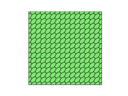
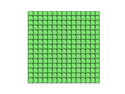
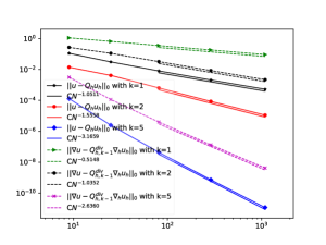
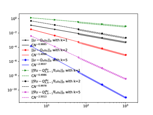
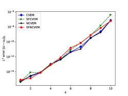
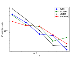
The rectangular domain is partitioned by the convex polygon mesh and non-convex polygon mesh in Fig. 1, respectively. We choose in both SFNCVEM and SFCVEM. The numerical results of the SFNCVEM on meshes and are shown in Fig. 2. We can see that and , which coincide with Theorem 4.9. And the numerical results of the SFCVEM are presented in Fig. 3. Again and , which confirm the theoretical convergence rate in Theorem 5.2.
6.2. The invertibility of the local stiffness matrices
We construct three different hexagons shown in Fig. 4, and calculate the eigenvalues of local stiffness matrices with for four virtual element methods. Our numerical results show that, on all the three hexagons, both SFNCVEM and SFCVEM have only one zero eigenvalue. In Tables 1-3, we also present the minimum non-zero eigenvalue, the maximum eigenvalue and the condition number for the local stiffness matrix on different hexagons in Fig. 4, from which we can see that these quantities are comparable for four virtual element methods.


| Method | Maximum eigenvalue | Minimum nonzero eigenvalue | Condition number |
|---|---|---|---|
| NCVEM | 975.5693189 | 0.309674737 | 3150.303211 |
| CVEM | 1012.488116 | 0.297206358 | 3406.683909 |
| SFNCVEM | 992.5956147 | 0.318932029 | 3112.248147 |
| SFCVEM | 1011.173331 | 0.298509692 | 3387.405362 |
| Method | Maximum eigenvalue | Minimum nonzero eigenvalue | Condition number |
|---|---|---|---|
| NCVEM | 935.2883848 | 0.279027715 | 3351.955143 |
| CVEM | 1014.672395 | 0.257370621 | 3942.456177 |
| SFNCVEM | 997.4831245 | 0.282126359 | 3535.589964 |
| SFCVEM | 1047.876056 | 0.258970708 | 4046.311124 |
| Method | Maximum eigenvalue | Minimum nonzero eigenvalue | Condition number |
|---|---|---|---|
| NCVEM | 941.8571938 | 0.21069027 | 4470.340249 |
| CVEM | 1046.755495 | 0.200435123 | 5222.4155 |
| SFNCVEM | 986.5963357 | 0.212761106 | 4637.108513 |
| SFCVEM | 1061.651989 | 0.202074633 | 5253.761808 |
6.3. Comparison of assembling time
The only difference between the standard VEMs and the VEMs without extrinsic stabilization is the stiffness matrix, so we compare the time consumed in assembling the stiffness matrix of four different VEMs in detail by varying the degree and the mesh size respectively. We use the mesh in Fig. 1(a) for this experiment. The results presented in Tables 4 and 5 show that NCVEM, CVEM and SFNCVEM have similar assembling time. However, SFCVEM requires more time due to the projection onto the one-order higher polynomial space.
| 2 | 4 | 8 | 10 | |
|---|---|---|---|---|
| SFCVEM | 0.053684235 | 0.144996881 | 1.468627453 | 2.603836536 |
| SFNCVEM | 0.022516727 | 0.065697193 | 0.806378841 | 1.554260015 |
| CVEM | 0.021185875 | 0.059809923 | 0.600241184 | 1.160929918 |
| NCVEM | 0.0213027 | 0.061014891 | 0.596506596 | 1.129639149 |
| 1 | 0.25 | 0.0625 | 0.03125 | |
|---|---|---|---|---|
| SFCVEM | 0.039689541 | 0.199015379 | 1.74412179 | 4.75462532 |
| SFNCVEM | 0.018287182 | 0.100006819 | 0.81251812 | 2.465409517 |
| CVEM | 0.018686771 | 0.087426662 | 0.781031132 | 1.983617783 |
| NCVEM | 0.018309593 | 0.096345425 | 0.767129898 | 2.159288645 |
6.4. Condition number of the stiffness matrix
We design two experiments to check the condition number of the stiffness matrices of the four VEMs.
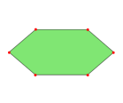
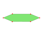
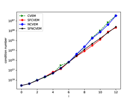
Firstly, we refer to the “collapsing polygons” experiment in [39] and consider a sequence of hexagons , where the vertices of are given by , , , , , and , where . The hexagons , and are drawn in Fig. 5. As shown in Fig. 6 for and , the condition numbers of stiffness matrices of the VEMs without extrinsic stabilization are smaller than those of the standard methods when is large.

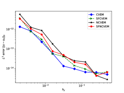
Secondly, we do the patch test for the Laplace equation, i.e. problem (4.1) with and , but the Dirichlet boundary condition is nonhomogeneous. Take the exact solution . Let and be mesh size in the -direction and -direction respectively. We examine the behavior of error of the four VEMs in the following three cases:
The errors of the four methods shown in Fig. 8 are similar. Since the error in the patch test grows as the condition number of the stiffness matrix grows, the condition numbers of the stiffness matrix obtained by four methods are comparable.
References
- [1] B. Ahmad, A. Alsaedi, F. Brezzi, L. D. Marini, and A. Russo. Equivalent projectors for virtual element methods. Comput. Math. Appl., 66(3):376–391, 2013.
- [2] A. Al-Taweel and X. Wang. The lowest-order stabilizer free weak Galerkin finite element method. Appl. Numer. Math., 157:434–445, 2020.
- [3] A. Al-Taweel and X. Wang. A note on the optimal degree of the weak gradient of the stabilizer free weak Galerkin finite element method. Appl. Numer. Math., 150:444–451, 2020.
- [4] A. Al-Taweel, X. Wang, X. Ye, and S. Zhang. A stabilizer free weak Galerkin finite element method with supercloseness of order two. Numer. Methods Partial Differential Equations, 37(2):1012–1029, 2021.
- [5] P. F. Antonietti, S. Berrone, A. Borio, A. D’Auria, M. Verani, and S. Weisser. Anisotropic a posteriori error estimate for the virtual element method. IMA J. Numer. Anal., 42(2):1273–1312, 2022.
- [6] D. Arnold and J. Guzmán. Local -bounded commuting projections in FEEC. ESAIM Math. Model. Numer. Anal., 55(5):2169–2184, 2021.
- [7] D. N. Arnold. Finite element exterior calculus, volume 93 of CBMS-NSF Regional Conference Series in Applied Mathematics. Society for Industrial and Applied Mathematics (SIAM), Philadelphia, PA, 2018.
- [8] D. N. Arnold, R. S. Falk, and R. Winther. Finite element exterior calculus, homological techniques, and applications. Acta Numer., 15:1–155, 2006.
- [9] B. Ayuso de Dios, K. Lipnikov, and G. Manzini. The nonconforming virtual element method. ESAIM Math. Model. Numer. Anal., 50(3):879–904, 2016.
- [10] L. Beirão da Veiga, F. Dassi, and A. Russo. High-order virtual element method on polyhedral meshes. Comput. Math. Appl., 74(5):1110–1122, 2017.
- [11] L. Beirão da Veiga, C. Lovadina, and A. Russo. Stability analysis for the virtual element method. Math. Models Methods Appl. Sci., 27(13):2557–2594, 2017.
- [12] L. Beirão da Veiga, F. Brezzi, A. Cangiani, G. Manzini, L. D. Marini, and A. Russo. Basic principles of virtual element methods. Math. Models Methods Appl. Sci., 23(1):199–214, 2013.
- [13] L. Beirão da Veiga, F. Brezzi, L. D. Marini, and A. Russo. The hitchhiker’s guide to the virtual element method. Math. Models Methods Appl. Sci., 24(8):1541–1573, 2014.
- [14] L. Beirão da Veiga, F. Brezzi, L. D. Marini, and A. Russo. Virtual element method for general second-order elliptic problems on polygonal meshes. Math. Models Methods Appl. Sci., 26(4):729–750, 2016.
- [15] S. Berrone, A. Borio, and F. Marcon. Lowest order stabilization free virtual element method for the Poisson equation. arXiv preprint arXiv:2103.16896, 2021.
- [16] S. Berrone, A. Borio, and F. Marcon. Comparison of standard and stabilization free virtual elements on anisotropic elliptic problems. Appl. Math. Lett., 129:Paper No. 107971, 5, 2022.
- [17] D. Boffi, F. Gardini, and L. Gastaldi. Approximation of PDE eigenvalue problems involving parameter dependent matrices. Calcolo, 57(4):Paper No. 41, 21, 2020.
- [18] S. C. Brenner. Poincaré-Friedrichs inequalities for piecewise functions. SIAM J. Numer. Anal., 41(1):306–324, 2003.
- [19] S. C. Brenner and L.-Y. Sung. Virtual element methods on meshes with small edges or faces. Math. Models Methods Appl. Sci., 28(7):1291–1336, 2018.
- [20] F. Brezzi, J. Douglas, Jr., R. Durán, and M. Fortin. Mixed finite elements for second order elliptic problems in three variables. Numer. Math., 51(2):237–250, 1987.
- [21] F. Brezzi, J. Douglas, Jr., and L. D. Marini. Recent results on mixed finite element methods for second order elliptic problems. In Vistas in applied mathematics, Transl. Ser. Math. Engrg., pages 25–43. Optimization Software, New York, 1986.
- [22] A. Cangiani, G. Manzini, and O. J. Sutton. Conforming and nonconforming virtual element methods for elliptic problems. IMA J. Numer. Anal., 37(3):1317–1354, 2017.
- [23] S. Cao, L. Chen, and R. Guo. Immersed virtual element methods for electromagnetic interface problems in three dimensions. Math. Models Methods Appl. Sci., 2023.
- [24] C. Chen, X. Huang, and H. Wei. -conforming virtual elements in arbitrary dimension. SIAM J. Numer. Anal., 60(6):3099–3123, 2022.
- [25] L. Chen and J. Huang. Some error analysis on virtual element methods. Calcolo, 55(1):55:5, 2018.
- [26] L. Chen and X. Huang. Nonconforming virtual element method for th order partial differential equations in . Math. Comp., 89(324):1711–1744, 2020.
- [27] L. Chen and X. Huang. Geometric decompositions of div-conforming finite element tensors. arXiv preprint arXiv:2112.14351, 2021.
- [28] L. Chen and X. Huang. Finite elements for div- and divdiv-conforming symmetric tensors in arbitrary dimension. SIAM J. Numer. Anal., 60(4):1932–1961, 2022.
- [29] L. Chen and X. Huang. Finite elements for conforming symmetric tensors in three dimensions. Math. Comp., 91(335):1107–1142, 2022.
- [30] P. G. Ciarlet. The finite element method for elliptic problems. North-Holland Publishing Co., Amsterdam, 1978.
- [31] M. Cicuttin, A. Ern, and S. Lemaire. A hybrid high-order method for highly oscillatory elliptic problems. Comput. Methods Appl. Math., 19(4):723–748, 2019.
- [32] M. Costabel and A. McIntosh. On Bogovskiĭ and regularized Poincaré integral operators for de Rham complexes on Lipschitz domains. Math. Z., 265(2):297–320, 2010.
- [33] F. Dassi and L. Mascotto. Exploring high-order three dimensional virtual elements: bases and stabilizations. Comput. Math. Appl., 75(9):3379–3401, 2018.
- [34] R. S. Falk and R. Winther. Local bounded cochain projections. Math. Comp., 83(290):2631–2656, 2014.
- [35] P. Grisvard. Elliptic problems in nonsmooth domains, volume 24 of Monographs and Studies in Mathematics. Pitman (Advanced Publishing Program), Boston, MA, 1985.
- [36] X. Huang. Nonconforming virtual element method for 2th order partial differential equations in with . Calcolo, 57(4):Paper No. 42, 38, 2020.
- [37] B. Hudobivnik, F. Aldakheel, and P. Wriggers. A low order 3D virtual element formulation for finite elasto-plastic deformations. Comput. Mech., 63(2):253–269, 2019.
- [38] P. D. Lax and A. N. Milgram. Parabolic equations. In Contributions to the theory of partial differential equations, Annals of Mathematics Studies, no. 33, pages 167–190. Princeton University Press, Princeton, N.J., 1954.
- [39] L. Mascotto. Ill-conditioning in the virtual element method: stabilizations and bases. Numer. Methods Partial Differential Equations, 34(4):1258–1281, 2018.
- [40] J.-C. Nédélec. Mixed finite elements in . Numer. Math., 35(3):315–341, 1980.
- [41] J.-C. Nédélec. A new family of mixed finite elements in . Numer. Math., 50(1):57–81, 1986.
- [42] J. Nečas. Les méthodes directes en théorie des équations elliptiques. Masson, Paris, 1967.
- [43] P.-A. Raviart and J. M. Thomas. A mixed finite element method for 2nd order elliptic problems. In Mathematical aspects of finite element methods (Proc. Conf., Consiglio Naz. delle Ricerche (C.N.R.), Rome, 1975), pages 292–315. Lecture Notes in Math., Vol. 606. Springer, Berlin, 1977.
- [44] R. Verfürth. A posteriori error estimation techniques for finite element methods. Numerical Mathematics and Scientific Computation. Oxford University Press, Oxford, 2013.
- [45] H. Wei, Y. Huang, and C. Chen. Fealpy: Finite element analysis library in python. https://github.com/weihuayi/fealpy, Xiangtan University, 2017-2023.
- [46] X. Xu and S. Zhang. A family of stabilizer-free virtual elements on triangular meshes. arXiv preprint arXiv:2309.09660, 2023.
- [47] X. Ye and S. Zhang. A stabilizer-free weak Galerkin finite element method on polytopal meshes. J. Comput. Appl. Math., 371:112699, 9, 2020.
- [48] X. Ye and S. Zhang. A stabilizer free weak Galerkin finite element method on polytopal mesh: Part II. J. Comput. Appl. Math., 394:Paper No. 113525, 11, 2021.
- [49] X. Ye and S. Zhang. A stabilizer free weak Galerkin finite element method on polytopal mesh: Part III. J. Comput. Appl. Math., 394:Paper No. 113538, 9, 2021.