Learning-Assisted Algorithm Unrolling for Online Optimization with Budget Constraints

Abstract

Online optimization with multiple budget constraints is challenging since the online decisions over a short time horizon are coupled together by strict inventory constraints. The existing manually-designed algorithms cannot achieve satisfactory average performance for this setting because they often need a large number of time steps for convergence and/or may violate the inventory constraints. In this paper, we propose a new machine learning (ML) assisted unrolling approach, called LAAU (Learning-Assisted Algorithm Unrolling), which unrolls the agent’s online decision pipeline and leverages an ML model for updating the Lagrangian multiplier online. For efficient training via backpropagation, we derive gradients of the decision pipeline over time. We also provide the average cost bounds for two cases when training data is available offline and collected online, respectively. Finally, we present numerical results to highlight that LAAU can outperform the existing baselines.

1 Introduction

Online optimization with budget (or inventory) constraints, also referred to as OOBC, is an important problem modeling a wide range of sequential decision-making applications with limited resources, such as online virtual machine resource allocation (Joe-Wong et al. 2013; Palomar and Chiang 2007), one-way trading in economics (El-Yaniv et al. 2001), resource management in wireless networks (Neely 2010; Lan et al. 2010), and data center server provisioning (Ghodsi et al. 2011). More specifically, when virtualizing a physical server into a small number of virtual machines (VMs) to satisfy the demand of multiple sequentially-arriving jobs, the agent must make sure that the total VM resource consumption is no more than what the physical server can provide (VMware 2022); additional examples can be found in Appendix B.

In an OOBC problem, online actions are selected sequentially to maximize the total utility over a short time horizon while the resource consumption over the time horizon is strictly constrained by a fixed amount of budgets (i.e., violating the budget constraint is naturally prohibited due to physical constraints). Consequently, the short time horizon (e.g., 24 hourly decisions in a day) and the strict budget constraint present substantial algorithmic challenges — the optimal solution relies on complete offline context information, but in the online setting, only the online contexts are revealed and the exact future contexts are unavailable for decision making (Lin et al. 2019, 2022).

A relevant but different problem is online optimization with (long-term) constraints (Balseiro, Lu, and Mirrokni 2020; Feldman et al. 2010; Neely 2010; Azar et al. 2016). In the literature, a common approach is to relax the long-term capacity constraints and include them as additional weighted costs into the original optimization objective, i.e., Lagrangian relaxation (Devanur et al. 2019; Zinkevich 2003; Balseiro, Lu, and Mirrokni 2020; Neely 2010). The Lagrangian multiplier can be interpreted as the resource price (Palomar and Chiang 2007), and is updated at each time step by a manually-designed algorithm such as Dual Mirror Descent (DMD) (Balseiro, Lu, and Mirrokni 2020; Wei, Yu, and Neely 2020; Jiang, Li, and Zhang 2020). These algorithms require a sufficiently long time horizon for convergence, which hence may not provide satisfactory performance for short-term budget constraints, especially when contexts in an episode are not identically independently distributed (i.i.d.). Additionally, some studies consider constraints on average (i.e., equivalently, long-term constraints) (Qiu et al. 2018; He et al. 2013) or bound the violation of the constraints (Neely 2010; Yu and Neely 2020; Sun et al. 2016). Thus, they do not apply to strict budget constraints over a short time horizon.

The challenges of OOBC with short-term and strict budget constraints can be further highlighted by that competitive online algorithms have only been proposed very recently under settings with linear constraints (Lin et al. 2019, 2022). Concretely, CR-Pursuit algorithms are proposed to make actions by following a pseudo-optimal algorithm based on the competitive ratio pursuit framework. Nonetheless, to make sure the solution exists for each OOBC episode, the guaranteed competitive ratio (ratio between the algorithm cost and the offline-optimal cost) can be very large. Also, they treat each OOBC problem instance as a completely new one and focus on the worst-case competitive ratio without considering the available historical data obtained when solving previous OOBC episodes. Thus, their conservative nature does not result in a satisfactory average performance, which limits the practicability of these algorithms.

By tapping into the power of historical data, a natural idea for OOBC is to train an machine learning (ML) based optimizer. Indeed, reinforcement learning has been proposed to solve online allocation problems in other contexts (Kong et al. 2019; Alomrani, Moravej, and Khalil 2021; Du, Wu, and Huang 2019). But, the existing ML-based algorithms for online optimization typically learn online actions in an end-to-end manner without exploiting the structure of the online problem being studied, which hence can have an unnecessarily high learning complexity and create additional challenges for generalization to unseen problem instances (Chen et al. 2021; Liu et al. 2019).

Contribution. We study OOBC with short-term and strict budget constraints, and propose a novel ML-assisted unrolling approach based on recurrent architectures, called LAAU (Learning-Assisted Algorithm Unrolling). Instead of using an end-to-end ML model to directly learn online actions, LAAU uniquely exploits the LAAU problem structure and unrolls the agent’s online decision pipeline into decision pipeline with three stages/layers — update the Lagrangian multiplier, optimize decisions subject to constraints, and update remaining resource budgets — and only plugs an ML model into the first stage (i.e., update the Lagrangian multiplier) where the key bottleneck for better performance exists. Thus, compared with the end-to-end model, LAAU benefits generalization by exploiting the knowledge of decision pipeline (Chen et al. 2021). Moreover, when the action dimension is larger than the number of constraints (i.e., the dimension of Lagrangian multipliers), the complexity advantage of using LAAU to learn Lagrangian multipliers can be further enhanced compared to learning the actions using an end-to-end model.

It is challenging to train LAAU through backpropagation since the constrained optimization layer is not easily differentiable. Thus, we derive tractable gradients for back-propagation through the optimization layer based on Karush-Kuhn-Tucker (KKT) conditions. In addition, we rigorously analyze the performance of LAAU in terms of the expected cost for both the case when the offline distribution information is available and the case when the data is collected online. Finally, to validate LAAU, we present numerical results by considering online resource allocation for maximizing the weighted fairness metric. Our results highlight that LAAU can significantly outperform the existing baselines and is very close to the optimal oracle in terms of the fairness utility.

2 Related Works

Constrained online optimization. Some earlier works (Devanur and Hayes 2009; Feldman et al. 2010) solve online optimization with (long-term) constraints by estimating a fixed Lagrangian multiplier using offline data. This approach works only for long-term or average constraints. Many other studies design online algorithms by updating the Lagrangian multiplier in an online style (Devanur et al. 2019; Balseiro, Lu, and Mirrokni 2020; Wei, Yu, and Neely 2020; Jiang, Li, and Zhang 2020). These algorithms guarantee sub-linear regrets under the i.i.d. context setting, and thus can achieve high utility if the number of time steps is sufficiently large. Likewise, the Lyapunov optimization approach addresses the long-term packing constraints by introducing virtual queues (equivalent to the Lagrangian multiplier) (Neely 2010; Yu and Neely 2020; Huang, Liu, and Hao 2014). Nonetheless, it also requires a sufficiently large number of time steps for convergence. By contrast, we consider online optimization with short-term strict budget constraints, which, motivated by practical applications, makes OOBC significantly more challenging.

Our work is relevant to the studies on OOBC (Lin et al. 2019, 2022) which design online algorithms to achieve a worst-case performance guarantee. However, to guarantee the worst-case performance and the feasibility of the algorithm, the algorithms are very conservative and their average performances are unsatisfactory. Comparably, we consider a more general setting where the budget constraint can be nonlinear, and utilize available historical data more efficiently to design ML-based LAAU that unrolls the online decision pipeline and achieves favorable average performance.

Algorithm unrolling. LAAU is related to the recent studies on ML-assisted algorithm unrolling and deep implicit layers, which integrate ML into traditional algorithmic frameworks for better generalization and interpretability, lower sampling complexity and/or smaller ML model size (Adler and Öktem 2018; Chen et al. 2021; Kolter, Duvenaud, and Johnson 2022; Monga, Li, and Eldar 2021; Liu et al. 2019). Algorithm unrolling has been used for sparse coding (Gregor and LeCun 2010; Sprechmann, Bronstein, and Sapiro 2015), signal and image processing (Monga, Li, and Eldar 2021; Li et al. 2019), and solving inverse problems (Kobler et al. 2020) and ordinary differential equations (ODEs) (Chen et al. 2018). Also, algorithm unrolling is applied in learning to optimize (L2O) (Chen et al. 2021; Wichrowska et al. 2017). Among these works, (Narasimhan et al. 2020) predicts the Lagrangian multiplier by a model to efficiently solve offline optimizations which may have a large number of constraints but allow constraint violations. These studies have their own challenges orthogonal to our problem where the key challenge is the lack of complete offline information. Thus, LAAU, to our knowledge, is the first to leverage ML to unroll an online optimizer for solving the online convex optimization with budget constraints, thus having better generalization than generic RL-based optimizers to directly obtain end solutions (Alomrani, Moravej, and Khalil 2021; Du, Wu, and Huang 2019; Kong et al. 2019).

3 Problem Formulation

As in the existing ML-based optimizers for online problems (Kong et al. 2019; Alomrani, Moravej, and Khalil 2021; Du, Wu, and Huang 2019), we consider an agent that interacts with a stochastic environment. The time horizon of an episode consists of $N$ time steps. For an episode, two vectors $\bm{c}=[c_{1},\cdots,c_{N}]^{\top}$ and $\bm{B}=[B_{1},\cdots,B_{M}]^{\top}$, where $c_{t}$ is a context vector and $B_{m}\in\mathbb{R}^{+}$ is the total budget for resource $m$, are drawn from a certain joint distribution $(\bm{c},\bm{B})\sim\mathcal{P}$, which we refer to as the environment distribution. Note that $c_{i}$ and $c_{j}$ for $i\not=j$ can follow different probability distributions, and so can $B_{i}$ and $B_{j}$ for $i\not=j$. The random vector $\bm{B}=[B_{1},\cdots,B_{M}]^{\top}$ are revealed at the beginning of an episode, and represents the budgets for $M$ types of resources. On the other hand, $\bm{c}=[c_{1},\cdots,c_{N}]^{\top}$ are online contexts sequentially revealed over $N$ different steps within an episode. That is, at step $t$, the agent only knows $c_{1},\cdots,c_{t}$, but not the future parameters $c_{t+1},\cdots,c_{N}$.

At each step $t=1,\cdots,N$, the agent makes a decision $x_{t}\in\mathbb{R}^{d}$, consumes some budgets, and also receives a utility. Given the decision $x_{t}$ and parameter $c_{t}$, the amount of the resource consumption is denoted as a non-negative function $g_{m}(x_{t},c_{t})\geq 0$, for $m=1,\cdots,M$. To be consistent with the notation of loss function, we use a cost or loss $l(x_{t},c_{t})$ to denote the negative of the utility — the less $l(x_{t},c_{t})$, the better. As the cost function $l(\cdot,c_{t})$ is parameterized by $c_{t}$, knowing $c_{t}$ is also equivalent to knowing the cost function. We assume that the loss function $l$ and the constraint functions $g_{m},m=1,\cdots,M$ are twice continuously differentiable, and either the loss function $l$ or one of the constraint functions $g_{m},m=1,\cdots,M$ is strongly convex in terms of the decision $x_{t}$.

For each episode with $(\bm{c},\bm{B})\sim\mathcal{P}$, the goal of the agent is minimizing its total cost over the $N$ steps subject to $M$ resource capacity constraints, which we formulate as follows:

$$\begin{split}&\min_{\bm{x}=(x_{1},\cdots,x_{N})}\sum_{t=1}^{N}l(x_{t},c_{t}),\\ &\text{ s.t. }\;\sum_{t=1}^{N}g_{m}(x_{t},c_{t})\leq B_{m},m=1,\cdots,M.\end{split}$$ (1)

This is an online optimization problem with inventory constraints (referred to as OOBC) in the sense that the short-term strict inventory constraints are imposed for each episode of $N$ time steps. An episode has its own $M$ capacity constraints which should be strictly satisfied, and the unused budgets cannot roll over to the next episode. For ease of notation, given a policy $\pi$ which maps available inputs to feasible actions, we denote $L(\pi)=\sum_{t=1}^{N}l(x_{t},c_{t})$ as the total loss for one episode and $\mathrm{E}\left[L(\pi)\right]$ as the expected total loss over the distribution of $(\bm{c},\bm{B})\sim\mathcal{P}$.

The setting of OOBC presents new technical challenges compared with existing works on constrained online optimization. Specifically in OOBC, the time horizon in an episode (episode length) is finite and can be very short. In this case, there are not many steps for algorithms to converge, and bad decisions at early steps have a large impact on the overall performance. Thus, DMD (Balseiro, Lu, and Mirrokni 2020; Wei, Yu, and Neely 2020; Jiang, Li, and Zhang 2020) and Lyapunov optimization (Neely 2010) which are specifically designed for long episodes may not provide good results for OOBC. Besides, unlike some studies that satisfy average constraints (Qiu et al. 2018; He et al. 2013) or that only approximately satisfy the constraints under bounded violations (i.e., soft constraints) (Yu and Neely 2020, 2019; Sun et al. 2016), OOBC requires all the constraints in Eqn. (1) be strictly satisfied. This requirement is necessary for many practical applications with finite available resources (e.g., a data center’s power capacity must not be exceeded (Fan, Weber, and Barroso 2007)), but makes the problem more challenging. Last but not least, the contexts in one episode in OOBC are drawn from a general joint distribution (not necessarily i.i.d.). Under non-i.i.d. cases, DMD(Balseiro, Lu, and Mirrokni 2020) has performance guarantees only when each episode is long enough. CR-Pursuit(Lin et al. 2019, 2022) has competitive ratios but is too conservative and may not perform well on average. To improve the average performance of OOBC, new algorithms are needed to effectively utilize history data of previous episodes.

4 Learning-Assisted Algorithm Unrolling

4.1 Relaxed Optimization

The design of LAAU is based on the Lagrangian relaxed optimization method which is introduced here. Since it is difficult to directly solve the constrained optimization in Eqn. (1) due to the lack of complete offline information in an online setting, many studies (Arora, Hazan, and Kale 2012; Balseiro, Lu, and Mirrokni 2020; Neely 2010) solve the Lagrangian relaxed form written as follows:

$$\begin{split}\min_{\bm{x}=(x_{1},\cdots,x_{N})}\sum_{t=1}^{N}l(x_{t},c_{t})+\lambda^{\top}\sum_{t=1}^{N}\bm{g}(x_{t},c_{t}),\end{split}$$ (2)

where $\bm{g}(x_{t},c_{t})=[g_{1}(x_{t},c_{t}),\cdots,g_{M}(x_{t},c_{t})]^{\top}$ and $\lambda=[\lambda_{1},\cdots,\lambda_{M}]^{\top}$ is the non-negative Lagrangian multiplier corresponding to the $M$ constraints $\sum_{t=1}^{N}\bm{g}(x_{t},c_{t})\leq\bm{B}$. The multiplier $\lambda$ with $M$ dimensions essentially relaxes the $M$ inventory constraints, thus decoupling the decisions over the $N$ time steps within an episode. It is also interpreted as the resource price in the resource allocation literature (Palomar and Chiang 2007; Boyd, Boyd, and Vandenberghe 2004; Neely 2010): A greater $\lambda_{t}$ means a higher price for the resource consumption, thus pushing the agent to use less resource. Clearly, had we known the optimal Lagrangian multiplier $\lambda^{*}$ at the beginning of each episode, the OOBC problem would become very easy. Unfortunately, knowing $\lambda^{*}$ also requires the complete offline information $(\bm{c},\bm{B})$, which is not possible in the online case. Nevertheless, if we can appropriately update $\lambda_{t}$ in an online manner while strictly satisfying the constraints, we can also efficiently solve the OOBC problem. Formally, by using $\lambda_{t}$ that is updated online for each step $t$, we can instead solve the following relaxed problem:

$$\begin{split}\min_{x_{t}}l(x_{t},c_{t})+\lambda_{t}^{\top}\bm{g}(x_{t},c_{t}),\;\text{ s.t., }\;\bm{g}(x_{t},c_{t})\leq\bm{b}_{t},\end{split}$$ (3)

where $\lambda_{t}=[\lambda_{t,1},\cdots,\lambda_{t,M}]^{\top}$, $\bm{g}(x_{t},c_{t})=[g_{1}(x_{t},c_{t}),\cdots,g_{M}(x_{t},c_{t})]^{\top}$, and the remaining budget for step $t$ is $\bm{b}_{t}=\bm{B}-\sum_{s=1}^{t-1}\bm{g}(x_{s},c_{s})$.

In fact, designing good update rules for $\lambda_{t}$ for each step $t=1,\cdots,N$ is commonly considered in the literature (Balseiro, Lu, and Mirrokni 2020; Agrawal and Devanur 2014). For example, (Balseiro, Lu, and Mirrokni 2020) update $\lambda_{t}$ by DMD, in order to meet long-term constraints while achieving a low regret compared to the optimal oracle. Nonetheless, it requires a large number of time steps to converge to a good Lagrangian parameter. Likewise, the Lyapunov optimization technique introduces a virtual queue, whose length essentially takes the role of $\lambda_{t}$ and is updated as $\lambda_{t+1}=\max\left\{\lambda_{t}+\bm{g}(x_{t},c_{t})-\frac{1}{N}\bm{B},0\right\}$ or in other similar ways (Neely 2010). Nonetheless, the convergence rate of using Lyapunov optimization is slow (even assuming $c_{t}$ is i.i.d. for $t=1,\cdots,N$), and there exists a tradeoff between cost minimization and long-term constraint satisfactory, making it unsuitable for the short-term constraints that we focus on.

Alternatively, one may want to exploit the distribution information of $(\bm{c},\bm{B})\sim\mathcal{P}$ and solve a relaxed problem offline by considering $M$ average constraints (referred to as AVG-LT). That is, we replace the short-term capacity constraints in Eqn. (1) with $\mathrm{E}_{\mathcal{P}}\left[\sum_{t=1}^{N}g_{m}(x_{t},c_{t})\right]\leq B_{m}$ for $m=1,\cdots,M$. By solving this relaxed problem, we can obtain a Lagrangian multiplier $\lambda_{\mathcal{P}}$ that only depends on $\mathcal{P}$ but not the specific $(\bm{c},\bm{B})$. Thus, we can replace $\lambda_{t}$ in Eqn. (3) with $\lambda_{\mathcal{P}}$. However, since this method uses a constant Lagrangian multiplier for all episodes, we will either be overly conservative and not using the budgets as much as possible, or violating the the constraints.

4.2 Algorithm Unrolling

Algorithm 1 Online Inference Procedure of LAAU

0:  ML model $f_{\theta}$.

1:  for t=1 to N do

2:     Receive $c_{t}$, forward propagate $f_{\theta}$ and get Lagrangian multiplier $\lambda_{t}=f_{\theta}\left(\bm{b}_{t},c_{t},\bar{t}\right)$.

3:     Solve the constrained convex optimization in (4) and make action $x_{t}$.

4:     Update the resource budget $\bm{b}_{t+1}=\bm{b}_{t}-\bm{g}(x_{t},c_{t})$.

5:  end for

We propose to leverage the powerful capacity of ML to find a solution. One approach is to train an end-to-end model that takes the online input information and directly outputs a decision. But, the end-to-end model should be large enough to capture the possibly complex logic of the optimal policy, and the end-to-end models often have poor interpretability and worse generalization (see the comparison between LAAU and the generic end-to-end approach in Section 7). Therefore, instead of replacing the whole decision pipeline with ML, we only plug an ML model in the most challenging stage — online updating of the Lagrangian multiplier $\lambda_{t}$ needed to solve the relaxed problem in Eqn. (3).

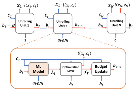
Figure 1: Architecture of LAAU. The red lines indicate the flows that need back propagation.

As shown in Algorithm 1 and illustrated in Fig. 1, the decision pipeline at step $t$ can be decomposed into three stages as follows.

Updating $\lambda_{t}$. At the beginning of step $t=1,\cdots,N$, the ML model takes the parameter $c_{t}$, the remaining budget $\bm{b}_{t}=[b_{t,1},\cdots,b_{t,m}]^{\top}$ and the normalized number of remaining steps $\bar{t}=\frac{N-t}{N}$ as the inputs, and outputs the Lagrangian multiplier $\lambda_{t}=[\lambda_{t,1},\cdots,\lambda_{t,m}]^{\top}$. Letting $f_{\theta}$ denote the ML model parameterized by $\theta$, we have $\lambda_{t}=f_{\theta}\left(\bm{b}_{t},c_{t},\bar{t}\right).$

Optimization layer. In the optimization layer, we solve a relaxed convex problem formulated in Eqn. (3). The natural constraints on the remaining resource budgets ensure that the strict inventory constraints are always satisfied by LAAU. We denote the optimization layer as $p(c_{t},\lambda_{t},\bm{b}_{t})$ and thus have:

$$\begin{split}x_{t}=p(c_{t},\lambda_{t},\bm{b}_{t})\!=&\!\arg\!\min_{x}\!\left(l(x,c_{t})+\lambda_{t}^{\top}\bm{g}(x,c_{t})\right),\\ &\text{ s.t., }\bm{g}(x,c_{t})\leq\bm{b}_{t}.\end{split}$$ (4)

Updating resource budgets. In the last stage, the remaining resource budgets serve as an input for the next recurrence and are updated as $\bm{b}_{t+1}=\bm{B}-\sum_{s=1}^{t}\bm{g}(x_{s},c_{s})=\bm{b}_{t}-\bm{g}(x_{t},c_{t})$.

Each episode includes $N$ recurrences, each for one decision step. The cost for step $t$ is calculated after the optimization layer as $l(x_{t},c_{t})$. Note that in the $N$-th recurrence which is the final stopping step, the remaining budget $\bm{b}_{r}=\bm{b}_{N}-\bm{g}(x_{N},c_{N})$ will be wasted if not used up. Thus, we directly set $\lambda_{N}=0$ for the $N$-th unrolling unit.

5 Training the Unrolling Architecture

To clearly explain the back propagation of the unrolling model, we first consider the offline training where offline distribution information is available. Then we extend to the online training setting where the data is collected online.

5.1 Offline Training

Training Objective

For the ease of notation, we denote the online optimizer as $\bm{h}_{\theta}\left(\bm{B},\bm{c}\right)$. For offline training, we are given an unlabeled training dataset $S=\left\{\left(\bm{c}_{1},\bm{B}_{1}\right),\cdots,\left(\bm{c}_{n},\bm{B}_{n}\right)\right\}$, with $n$ samples of $(\bm{c},\bm{B})$. The training dataset can be synthetically generated by sampling from the target distribution for the online input $(\bm{c},\bm{B})$, which is a standard technique in the context of learning to optimize (Chen et al. 2021; Dai et al. 2017; Li and Malik 2017; Alomrani, Moravej, and Khalil 2021; Du, Wu, and Huang 2019). By forward propagation, we can get the empirical training loss as $L(\bm{h}_{\theta},S)=\frac{1}{n}\sum_{i=1}^{n}\sum_{t=1}^{N}l(\bm{x}_{i,t},\bm{c}_{i,t})$ where $\bm{x}_{i,t}$ is the output of the online optimizer $\bm{h}_{\theta}$ regarding $\bm{c}_{i}$ and $\bm{B}_{i}$. By minimizing the empirical loss, we get $\hat{\theta}=\arg\min_{\theta}L(\bm{h}_{\theta},S)$.

Backpropagation

Typically, the minimization of the training loss is performed by gradient descent-based algorithms like SGD or Adam, which need back propagation to get the gradient of the loss with respect to the ML model weight $\theta$. Nonetheless, unlike standard ML training (e.g., neural network training with only linear and activation operations), our unrolled recurrent architecture includes an implicit layer — the optimization layer (Kolter, Duvenaud, and Johnson 2022). Additionally, the unrolling architecture has multiple skip connections. Thus, the back-propagation process is dramatically different from that of standard recurrent neural networks. Next, we derive the gradients for back propagation in our unrolling design. Note that the loss $l(x_{t},c_{t})$ for any $t=1,\cdots,N$ is directly determined by the output of the optimization layer $x_{t}$ and the parameter $c_{t}$, and $x_{t}$ needs back propagation. Thus, by the chain rule, we have

$$\bigtriangledown_{\theta}l\!\left(x_{t},c_{t}\right)\!\!=\!\!\bigtriangledown_{x_{t}}\!l\!\left(x_{t},c_{t}\right)\!\!\left(\!\bigtriangledown_{\lambda_{t}}\!x_{t}\!\!\bigtriangledown_{\theta}\lambda_{t}\!\!+\!\!\bigtriangledown_{\bm{b}_{t}}\!x_{t}\!\!\bigtriangledown_{\theta}\bm{b}_{t}\right).$$ (5)

To get $\bigtriangledown_{\lambda_{t}}\!x_{t}$ and $\bigtriangledown_{\bm{b}_{t}}\!x_{t}$ in Eqn. (5), we need to perform back propagation for the optimization layer $p(c_{t},\lambda_{t},\bm{b}_{t})$. This is a challenging task and will be addressed in Section 5.1. The other gradients in Eqn. (5) include $\bigtriangledown_{\theta}\lambda_{t}$ and $\bigtriangledown_{\theta}\bm{b}_{t}$. Note that $\lambda_{t}$, which is the ML model output directly determined by its ML model weight $\theta$, and the remaining budget $\bm{b}_{t}$ both need back propagation. Thus, the gradient of $\lambda_{t}$ with respect to the ML model weight $\theta$ is expressed as

$$\bigtriangledown_{\theta}\lambda_{t}=\bigtriangledown_{\theta}f_{\theta}\left(\bm{b}_{t},c_{t},\bar{t}\right)+\bigtriangledown_{\bm{b}_{t}}f_{\theta}\left(\bm{b}_{t},c_{t},\bar{t}\right)\bigtriangledown_{\theta}\bm{b}_{t},$$ (6)

Now, it remains to derive $\bigtriangledown_{\theta}\bm{b}_{t}$, which is important since $b_{t}$ is the signal connecting two adjacent recurrences. By the expression of $b_{t}$ in Line 4 of Algorithm 1, we have

$$\bigtriangledown_{\theta}\bm{b}_{t}=\bigtriangledown_{\theta}\bm{b}_{t-1}+\bigtriangledown_{x_{t-1}}\bm{g}(x_{t-1},c_{t-1})\bigtriangledown_{\lambda_{t-1}}\!x_{t-1}\bigtriangledown_{\theta}\lambda_{t-1},$$ (7)

Combining Eqn. (5), (6) and (7), we get the recurrent expression for back propagation. Then, by adding up the gradients of the losses over $N$ time steps, we get the gradient of the total loss as $\bigtriangledown_{\theta}L(\bm{h}_{\theta},S)=\frac{1}{n}\sum_{i=1}^{n}\sum_{t=1}^{N}\bigtriangledown_{\theta}l\left(x_{i,t},c_{i,t}\right)$.

Differentiating the Optimization Layer

It is challenging to get the close-form solution and its gradients for many constrained optimization problems. One possible remedy is to use some black-box gradient estimators like zero-order optimization (Liu et al. 2020; Ruffio et al. 2011). However, zero-order gradient estimators are not computationally efficient since many samples are needed to estimate a gradient. Another method is to train a deep neural network to approximate the optimization layer in Eqn. (4) and then calculate the gradients based on the neural network. However, we need many samples to pre-train the neural network, and the gradient estimation error can be large. we analytically differentiate the solution to Eqn. (4) in the optimization layer with respect to the inputs $\lambda_{t}$, and $\bm{b}_{t}$ by exploiting KKT conditions (Kolter, Duvenaud, and Johnson 2022; Boyd, Boyd, and Vandenberghe 2004). The KKT-based differentiation method, given in Proposition 5.1, is computationally efficient, explainable and accurate (under mild technical conditions).

Proposition 5.1 (Back-propagation by KKT).

Assume that $x_{t}$ and $\mu_{t}$ are the primal and dual solutions to Eqn. (4) , respectively. Let $\Delta_{11}=\bigtriangledown_{x_{t}x_{t}}l\left(x_{t},c_{t}\right)+\sum_{m=1}^{M}\left(\lambda_{m,t}+\mu_{m,t}\right)\!\!\bigtriangledown_{x_{t}x_{t}}g_{m}\!\left(x_{t},c_{t}\right)$, $\Delta_{12}=\left[\bigtriangledown_{x_{t}}\bm{g}\left(x_{t},c_{t}\right)\right]^{\top}$, $\Delta_{21}=\mathrm{diag}(\mu_{t})\bigtriangledown_{x_{t}}\bm{g}\left(x_{t},c_{t}\right)$, and $\Delta_{22}=\mathrm{diag}\left(\bm{g}\left(x_{t},c_{t}\right)-\bm{B}_{t}\right)$. If the conditions in Proposition 5.2 are satisfied, the gradients of the optimization layer w.r.t. $\lambda_{t}$ and $\bm{b}_{t}$ are

$$\bigtriangledown_{\lambda_{t}}x_{t}=-\left(\Delta_{11}^{-1}+\Delta_{11}^{-1}\Delta_{12}\mathrm{Sc}\left(\Delta,\Delta_{11}\right)^{-1}\Delta_{21}\Delta_{11}^{-1}\right)\Delta_{12},$$

$$\bigtriangledown_{\bm{b}_{t}}x_{t}=-\Delta_{11}^{-1}\Delta_{12}\mathrm{Sc}\left(\Delta,\Delta_{11}\right)^{-1}\mathrm{diag}(\mu_{t}),$$

where $\mathrm{Sc}\left(\Delta,\Delta_{11}\right)=\Delta_{22}-\Delta_{21}\Delta^{-1}_{11}\Delta_{12}$ denotes the Shur-complement of $\Delta_{11}$ in $\Delta=\left[[\Delta_{11},\Delta_{12}];[\Delta_{21},\Delta_{22}]\right]$. $\hfill{\square}$

We find that to get truly accurate gradient computation by Proposition 5.2, the Shur-complement $\mathrm{Sc}\left(\Delta,\Delta_{11}\right)$ and $\Delta_{11}$ should be invertible. Otherwise, we can get approximated gradients by taking pseudo-inverse of $\mathrm{Sc}\left(\Delta,\Delta_{11}\right)$ and $\Delta_{11}$. The sufficient conditions to guarantee perfectly accurate gradient computation are given in Proposition 5.2.

Proposition 5.2 (Sufficient Conditions of Accurate Differentiation).

Assume that the problem in Eqn. (4) satisfies strong duality. The loss $l$ or one of the constraints $g_{m},m=1,\cdots,M$ is strongly convex with respect to $x$. Denote $\mathcal{A}$ as the index set of constraints that are activated (i.e., equality holds) under the optimal solution. $\mu_{m,t}\neq 0,\forall m\in\mathcal{A}$, the size of the activation set satisfies $|\mathcal{A}|\leq d$ with $d$ as the action dimension, and the gradients $\bigtriangledown_{x_{t}}g_{m}(x_{t}),m\in\mathcal{A}$ are linearly independent and not zero vectors, the gradients in Proposition 5.1 are perfectly accurate.

Remark 1.

To derive the gradient of Eqn. (4) with respect to an input parameter, we take gradients on both sides of the equations in KKT conditions by the chain rule and get new equations about the gradients. By solving the obtained set of equations and exploiting the block matrix inversion, we can derive the gradients with respect to the inputs in Proposition 5.1.

The conditions in Proposition 5.2 are mild in practice. First, strong duality is easily satisfied for the considered convex optimization in Eqn. (4) given the Slater’s condition (Boyd, Boyd, and Vandenberghe 2004). Besides, the requirement of strong convexity excludes linear programming (LP). Actually, LP problems with resource constraints are usually solved by other relaxations other than our considered relaxation in Eqn. (2) (Devanur et al. 2019). The other conditions are related to activated constraints. According to the condition of complementary slackness (Boyd, Boyd, and Vandenberghe 2004), the condition that optimal dual variables corresponding to the activated constraints are not zero typically holds. We also require that the number of activated constraints is less than the action dimension, and the gradient vectors of the activated constraint functions under optimal solutions should be independent from each other. Given that at most a small number of constraints are activated in most cases, the two conditions are easily satisfied. Actually, the independence condition requires that the activated constraints are not redundant — an activated constraint function is not a linear combination of any other activated constraint functions; otherwise, it can be replaced by other constraints. The proof of Proposition 5.2 is given in the appendix D.

5.2 Online Training

In practice, we may have a cold-start setting without many offline samples. An efficient approach for this setting is online stochastic gradient descent (SGD) with its algorithm in Appendix A. Concretely, when the $i$-th instance arrives, we perform online inference by Algorithm 1. After the instance with $N$ steps ends, we collect the context and budget data of this episode and update the ML model weight $\hat{\theta}_{i}$ by performing one-step gradient descent, i,e, $\hat{\theta}_{i}=\hat{\theta}_{i-1}-\bar{\alpha}\triangledown_{\theta}L(h_{\hat{\theta}_{i-1}},\bm{c}_{i})$ where $L(h_{\hat{\theta}_{i-1}},\bm{c}_{i})$ is the loss of the unrolling model for the $i$th instance and $\bar{\alpha}$ is the stepsize. The back propagation method is the same as the offline training. Then, with the updated $\hat{\theta}_{i}$, we perform inference by Algorithm 1 for the instance in the $(i+1)$-th round. We will show by analysis that the average cost decreases with time.

6 Performance Analysis

In this section, we bound the expected cost when the trained ML model $f_{\theta}$ is used in LAAU.

Definition 1.

The weight in the ML model $f_{\theta}$ (and also the online optimizer $\bm{h}_{\theta}$) that minimizes the expected loss $\mathrm{E}\left[L(\bm{h}_{\theta},\bm{c})\right]$ with respect to the distribution of $(\bm{c},\bm{B})\sim\mathcal{P}$ is defined as $\theta^{*}=\arg\min_{\theta\in\Theta}\mathrm{E}\left[L(\bm{h}_{\theta},\bm{c})\right],$ and the weight that minimizes the empirical loss $L(\bm{h}_{\theta},S)$ is defined as $\hat{\theta}^{*}=\arg\min_{\theta\in\Theta}L(\bm{h}_{\theta},S),$ where $\Theta$ is the weight space.

In Definition 1, given the weight space $\Theta$, $\bm{h}_{\theta^{*}}$ is the best online optimizer based on the unrolling architecture in terms of the expected cost. $\bm{h}_{\theta^{*}}$ is not the offline-optimal policy, but it is close to the policy that performs best given available online information when the capacity of the ML model and weight space $\Theta$ are large enough. Next, we show the performance gap of LAAU compared with $h_{\theta^{*}}$.

Theorem 6.1.

By the optimization layer in Eqn. (4), LAAU satisfies the inventory constraints for each OOBC instance. Suppose that $\hat{\theta}$ is the ML model weight by offline training on dataset $S$ with $n$ samples, and that we plug it into the online optimizer $\bm{h}_{\hat{\theta}}$. With probability at least $1-\delta,\delta\in(0,1)$,

$$\begin{split}\mathrm{E}\left[L(\bm{h}_{\hat{\theta}})\right]\!\!-\!\!\mathrm{E}\left[L(\bm{h}_{\theta^{*}})\right]\leq\mathcal{E}\left(\bm{h}_{\hat{\theta}},S\right)+4R_{n}(L\circ\mathbb{H})\\ +2\left(\Gamma_{L,c}\omega_{c}+\Gamma_{L,b}\omega_{b}\right)\sqrt{\frac{\ln(2/\delta)}{n}},\end{split}$$ (8)

where $\mathcal{E}\left(\bm{h}_{\hat{\theta}},S\right)=L(\bm{h}_{\hat{\theta}},S)-L(\bm{h}_{\hat{\theta}^{*}},S)$ is the training error, $R_{n}(L\circ\mathbb{H})$ is the Rademacher complexity regarding the loss space $L\circ\mathbb{H}=\left\{L(\bm{h}),\bm{h}\in\mathbb{H}\right\}$ with $\mathbb{H}$ being the ML model set, $\omega_{c}=\max_{\bm{c},\bm{c}^{\prime}\in\mathbb{C}}\left\|\bm{c}-\bm{c}^{\prime}\right\|$ is the size of the parameter space $\mathbb{C}$, $\omega_{b}=\max_{\bm{B},\bm{B}^{\prime}\in\mathbb{B}}\left\|\bm{B}-\bm{B}^{\prime}\right\|$ is the size of the capacity constraint space $\mathbb{B}$, $\Gamma_{L,c}$ and $\Gamma_{L,b}$ are the Lipschitz constants of the total loss $L(\bm{h}_{\theta},\bm{c})=\sum_{t=1}^{N}l(x_{t},c_{t})$ with respect to $\bm{c}$ and $\bm{B}$, respectively.

Proposition 6.2.

If a linear model $f_{\theta}(\bm{v})=\theta^{\top}\phi(\bm{v}),\|\theta\|\leq Z$ is used as the ML model in LAAU, the Rademacher complexity $R_{n}(L\circ\mathbb{H})$ is bounded ny $O\left(\frac{ZW}{\sqrt{n}}\right),$ where $W=\sup_{\bm{v}}\sqrt{\phi(\bm{v})^{\top}\phi(\bm{v}})$. If a neural network, where the depth is $K$, the width is less than $u$, activation functions are $\Gamma_{\alpha}$-Lipschitz continuous, and the spectrum norm of the weight matrix in layer $k$ with is less than $Z_{k}$, is used as the ML model, the Rademacher complexity $R_{n}(L\circ\mathbb{H})$ is bounded by $R_{n}(L\circ\mathbb{H})\leq O\left(\frac{K^{3/2}u\Gamma_{\alpha}(\beta_{b}+\beta_{c})\prod_{k=1}^{K}Z_{k}}{\sqrt{n}}\right),$ where $\beta_{b},\beta_{c}$ are the largest $l_{2}$-norm of $\bm{B}$ and $\bm{c}$. The notation $O$ in this proposition indicates the scaling relying on $M$, $N$, the Lipschitz constants of loss function $l$, constraint function $g$, optimization layer $p$ and neural network $f$.

Remark 2.

Theorem 6.1 shows that the performance gap between LAAU and the pseudo-oracle $h_{\theta^{*}}$ in terms of expected loss is bounded by the empirical training error, plus a generalization error which relies on the Radmacher complexity, the LipSchitz constant of the online optimizer, and the number of training samples. The Radmacher complexity indicates the richness of the loss function space with respect to the online optimizer space $\mathbb{H}$ and the distribution $\mathcal{P}$ and is further bounded in Proposition 6.2. From the bound of Radmacher complexity, we find that for both linear model and neural network, the generalization error increases with episode length $N$ and the number of constraints $M$. Besides, the Rademacher complexity relies on the ML model designs. For example, if a linear model is used as the ML model, the generalization error relies on the norm bounds of feature mapping and linear weights, while if a neural network is used as the ML model, the generalization error is related to the network length , width, the smoothness of activation functions, and spectral norm bounds of the weights in each layer. The last term of the expected cost bound is scaled by $\left(\Gamma_{L,c}\omega_{c}+\Gamma_{L,b}\omega_{b}\right)$ which indicates the sensitivity of the loss when the inputs are changed. This term highly depends on the Lipschitz constants of the total loss regarding the two inputs. Our proof in the appendix gives the bound of the Lipschitz constants of the loss regarding its inputs. $\square$

Proposition 6.3 (Average Cost of Online Training).

Assume that for each round $i$, $\triangledown_{\theta}\mathrm{E}[L(h_{\hat{\theta}_{i}})]$ is $\Gamma_{\triangledown L,\theta}$-Lipschitz continuous, and the Polyak-Lojasiewicz inequality is satisfied, i.e. $\exists\varsigma>0,\left\|\triangledown_{\theta}\mathrm{E}[L(h_{\hat{\theta}_{i}})]\right\|^{2}\geq 2\varsigma\left(\mathrm{E}[L(h_{\hat{\theta}_{i}})]-\mathrm{E}[L(h_{\theta^{*}})]\right)$. Also, assume that for the distribution of $\bm{c}_{i},$, $\exists\iota_{G}>\iota>0$ such that $\forall i$, $\left\langle\triangledown_{\theta}\mathrm{E}[L(h_{\hat{\theta}_{i}})],\mathrm{E}\left[\triangledown_{\theta}L(h_{\hat{\theta}_{i}},\bm{c}_{i})\right]\right\rangle\geq\iota\left\|\triangledown_{\theta}\mathrm{E}[L(h_{\hat{\theta}_{i}})]\right\|^{2}_{2}$, $\|\mathrm{E}[\triangledown_{\theta}L(h_{\hat{\theta}_{i}},\bm{c}_{i})]\|_{2}\leq\iota_{G}\left\|\triangledown_{\theta}\mathrm{E}[L(h_{\hat{\theta}_{i}})]\right\|_{2}$, and there exist $\varpi,\varpi_{V}>0$ such that $\forall i$, $\mathrm{Var}\left[\triangledown_{\theta}L(h_{\hat{\theta}_{i}},\bm{c}_{i})\right]\leq\varpi+\varpi_{V}\left\|\triangledown_{\theta}\mathrm{E}[L(h_{\hat{\theta}_{i}})]\right\|^{2}_{2}$. Then with the same notations as Theorem 6.1, for the online setting where LAAU is trained by SGD with stepsize $0<\bar{\alpha}\leq\frac{\iota}{\Gamma_{\triangledown L,\theta}(\varpi_{V}+\iota_{G}^{2})}$, with probability at least $1-\delta,\delta\in(0,1)$, we have for each round $i$

$$\begin{split}\!\mathrm{E}\!\left[\!L(\bm{h}_{\hat{\theta_{i}}})\!-\!L(\bm{h}_{\theta^{*}})\right]\!\leq\!\frac{\bar{\alpha}\Gamma_{\triangledown L,\theta}\varpi}{2\iota\varsigma}+O\left(\left(1-\bar{\alpha}\iota\varsigma\right)^{i}\right),\end{split}$$ (9)

where the expectation is taken over the randomness of context $\bm{c}$ and budget $\bm{B}$ and the model weight $\hat{\theta}_{i}$ by SGD.

Proposition 6.3, with proof in appendix E, bounds the expected loss gap between the learned weight $\hat{\theta}_{i}$ by SGD and the optimal weight $\theta^{*}$ defined in Definition 1. The first non-reducible term is caused by the randomness of the context and budget $\{(\bm{c}_{i},\bm{B}_{i})\}$. The second term decreases with time and the convergence rate depends on the randomness of the sequence and the parameter $\varsigma$ in the Polyak-Lojasiewicz inequality.

7 Numerical Results

Weighted fairness is a classic performance metric in the resource allocation literature (Lan et al. 2010), including fair allocation in computer systems (Ghodsi et al. 2011) and economics (Hylland and Zeckhauser 1979). Here, we consider a general online setting. A total of $N$ jobs arrive sequentially, and job $t$ has a weight $c_{t}\geq 0$. The agent allocates resource $x_{t}\geq 0$ to job $t$ at each step $t$. We consider the commonly-used weighted fairness $\sum_{t=1}^{N}c_{t}\log(x_{t})$ (Lan et al. 2010). We create the training and testing samples based on the Azure cloud workload dataset, which contains the average CPU reading for tasks at each step (Shahrad et al. 2020). For detailed settings, please refer to the appendix C.

We consider several baseline algorithms as follows. The Offline Optimal Oracle OPT is the solution to the problem in Eqn. (1). We consider two heuristics: One is Equal Resource Allocation (Equal) which equally allocates the total resource capacity to $N$ jobs, and another one is Resource Allocation with Average Long-term Constraints (AVG-LT) which relaxes the inventory constraints of the weighted fairness problem as $\mathrm{E}_{\mathcal{P}}\left[\sum_{t=1}^{N}x_{t}\right]\leq B$ and uses the optimal Lagrangian multiplier for this relaxed problem as $\lambda_{t}$ for online allocation. We consider two algorithms based on dual mirror descent which are Dual Gradient Descent (DGD) and Multiplicative Weight (MW ) (Balseiro, Lu, and Mirrokni 2020). To reduce the resource waste after the last step, we slightly revise DGD and MW by setting the allocation decision for job $N$ as $\min\left(b_{N},x_{\max}\right)$. CR-pursuit (CR-pursuit) is the state-of-the-art online algorithm that makes online actions by tracking a pseudo-optimal algorithm with a competitive guarantee (Lin et al. 2019, 2022). We also compare LAAU with the end-to-end Reinforcement Learning (RL). A neural network with the same size of the ML model as in LAAU is used in RL to directly predict the solution $x_{t}$, given parameter $c_{t}$ and budget $b_{t}$ as inputs.

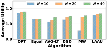
Figure 2: Average utility with different episode lengths

Average utility. We first show in Fig. 2 the average utilities (per time step). We do not add the average utility of CR-pursuit in the figure because its average utility for our evaluation instances is as low as 0.562, exceeding the utility range of the figure. Clearly, OPT achieves the highest utility, but it is infeasible in practice due to the lack of complete offline information. We can observe that the average utilities by expert algorithms including AVG-LT, DGD, MW are even below the average utility by the simple equal allocation (Equal) when the episode length is $N=10$. This is because all the three algorithms are designed for online optimizations with long-term constraints, and not suitable for the more challenging short-term counterparts. By contrast, LAAU performs well for all cases with large and small episode lengths, and outperforms the other algorithms designed for long-term constraints even when $N$ is as large as 40. This demonstrates the power of LAAU in solving challenging online problems with inventory constraints. More results, including detailed comparisons between LAAU and RL, are given in the appendix C.

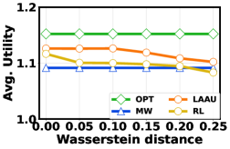
Figure 3: Average utility with different Wasserstein distances.

OOD testing. In practice, the training-testing distributional discrepancy is common and decreases ML model performance. We measure the training-testing distributional difference by the Wasserstein distance $d_{W}$. We choose the setting with episode length $N=20$ to perform the OOD evaluation. To create the distributional discrepancy, we add i.i.d. Gaussian noise with different means and variances to the training data and keep the testing data the same as the default setting. The distributions with different Wasserstein distances is visualized by t-SNE (Maaten and Hinton 2008) in the appendix C. The offline optimal and MW do not make use of the training distribution, and hence are not affected. We can see in Fig. 3 that, the OOD testing decreases the performance of both LAAU and RL, but LAAU is less affected by OOD testing than RL and is still higher than that of the baseline MW even under large Wasserstein distance. This is because the unrolling architecture in LAAU has an optimization layer and a budget update layer, which are deterministic and have no training parameters, so only the ML model to learn the Lagrangian multiplier is affected by OOD testing. Comparably, RL uses an parameterized end-to-end policy model trained on the offline data, so it has worse performance under OOD testing. This highlights that by the unrolling archietecture, LAAU has better generalization performance than end-to-end models.

8 Conclusion

In this paper, we focus on OOBC and propose a novel ML-assisted unrolling approach based on the online decision pipeline, called LAAU. We derive the gradients for back-propagation and perform rigorous analysis on the expected cost. Finally, we present numerical results on weighted fairness and highlight LAAU significantly outperforms the existing baselines in terms of the average performance.

Appendix

Appendix A Online Training Algorithm

The online training method in Section 5.2 is given in the following algorithm.

Algorithm 2 Online Training of LAAU

1:  Initialization: The weight $\hat{\theta}_{0}$ of the unrolling model, step size $\bar{\alpha}$.

2:  while a new instance $i$ arrives do

3:     Perform $N$-step online inference by Algorithm 1.

4:     Collect context $\bm{c}_{i}$ and budget $\bm{B}_{i}$ of instance $i$ and update the model by

$$\hat{\theta}_{i}=\hat{\theta}_{i-1}-\bar{\alpha}\triangledown_{\theta}L(h_{\hat{\theta}_{i-1}},\bm{c}_{i}),$$

where $\triangledown_{\theta}L(h_{\hat{\theta}_{i-1}},\bm{c}_{i})$ is obtained by back propagation in Eqn. (5).

5:  end while

Appendix B Motivating Examples

We now present the following motivating examples to highlight the practical relevance of OOBC.

B.1 Virtual machine resource allocation

Server virtualization plays a fundamental role in cloud computing, reaping the multiplexing benefits and improving resource utilization (VMware 2022). Each physical server has its own resource configuration, including CPU, memory, I/O and storage, and is virtualized into $N$ VMs. Jobs arrive sequentially in an online manner and each needs to be allocated with a VM. Thus, VM resource allocation is a crucial problem, affecting the job performance such as latency and throughput, as well as the resource consumption. The whole resource allocation process for $N$ VMs hosted on one physical server can be viewed as an episode in our problem formulation, while resource allocation for each individual VM is a per-step online decision. The job features, e.g., data size, are the online parameters revealed to the resource manager. Given the online job arrivals, the goal of the agent is to optimize a certain metric of interest, such as the total throughput and fairness. Crucially, the per-server resource constraints must be satisfied, resulting in short-term constraints as considered in our problem.

B.2 Rate allocation in unreliable wireless networks

Unlike wired networks, wireless networks are unreliable and subject to intermittent availability due to various factors such as background interference, fading, congestion, and/or priority-based spectrum access. Here, we use cognitive radio networks as an example, which provide an important mechanism to improve the utilization of increasingly wireless spectrum by allowing unlicensed users to opportunistically access the available spectrum unoccupied by licensed users (Haykin 2006). Due to the random time-varying spectrum usage by licensed users, the available spectrum $\bm{B}$ for unlicensed users is thus also random: it is available for only one fixed period of time (i.e., an episode), but may change later. During each time period, $N$ unlicensed users submit their spectrum access requests to the spectrum manager in an online manner at the moment when their own traffic becomes available. Each user’s traffic is associated with a parameter $c_{t}$, which indicates the $t$-th user’s features such as priority and channel condition. The spectrum manager makes a decision $x_{t}$, specifying the rate allocation to user $t$. This decision results in a wireless bandwidth usage that depends on the user’s channel condition, as well as a utility. The goal of the spectrum manager is to maximize the total utility for these $N$ users subject to the total available bandwidth constraint.

Appendix C Simulation Settings and Additional Empirical Results

C.1 Experiment Setups

Problem Setup

In this section, we give more details about the application and simulation settings of online weighted fairness. We consider a general online resource allocation setting with a total of $N$ jobs arrive sequentially, and job $t$ has a weight $c_{t}\geq 0$, which is not known to the agent until the step $t$. The agent allocates resource $x_{t}\geq 0$ to job $t$ at each step $t$, without knowing the weights for future jobs. At the beginning of step $t=1$, the agent is also informed of a total resource capacity/budget of $B$ that can be allocated over $N$ time steps. To measure the resource allocation fairness (Lan et al. 2010), we consider a commonly-used utility $\sum_{\tau=1}^{N}c_{\tau}\log(x_{\tau})$, where $\log$ is the natural logarithm, $\bm{x}=[x_{1},\cdots,x_{N}]$ and $\bm{c}=[c_{1},\cdots,c_{N}]$. Therefore, the problem of online resource allocation for weighted fairness with short-term capacity constraints is to maximize the fairness utility subject to the resource constraints:

$$\begin{split}\max_{\bm{x}}\sum_{t=1}^{N}c_{t}\log(x_{t}),\text{ s.t. }\sum_{t=1}^{N}x_{t}\leq B\text{ and }x_{t}\in\left[x_{\min},x_{\max}\right],\end{split}$$ (10)

where $x_{\max}=40$ and $x_{\min}=1$ (to ensure a non-negative utility) represent the lowest and highest amounts of resource that can be allocated to each job.

Datasets

We perform simulations for the settings with different lengths $N$, which is chosen from $\left\{10,20,40\right\}$. By default, we set $N=20$. We use the the cloud dataset (Shahrad et al. 2020) for simulation. The cloud dataset is a dataset of workload sequences which are $\bm{c}$ in our formulations. The workload sequences in the cloud dataset are divided into multiple problem instances, each with $N$ time steps, and the workload at step $t$ is $c_{t}$. In each instance, the total resource capacity/budget is drawn from an independent and uniform distribution in the range $[10N,15N]$, where $N$ is the number of time steps in each episode. We use 5000 offline problem instances for training and 1000 instances for validation. For testing, we use another 2000 problem instances from the cloud dataset to evaluate the performances of different algorithms. In the default setting, the training problem instances are drawn from the same distribution as the testing distribution, but we will also change the distribution when evaluating the OOD cases.

(a) Default.

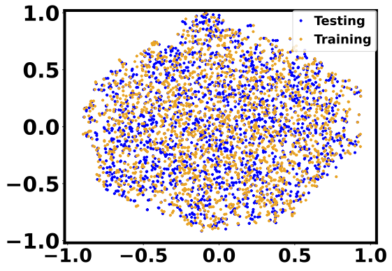
(b) $d_{W}=0.05$

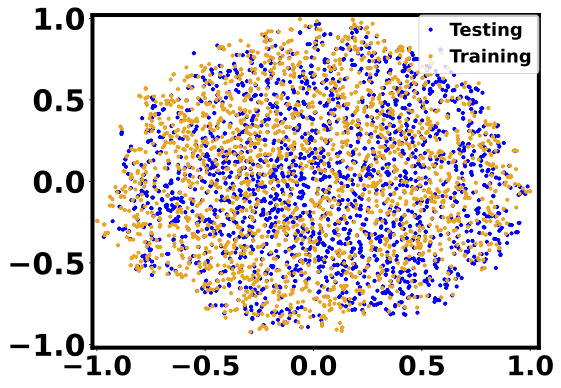
(c) $d_{W}=0.1$

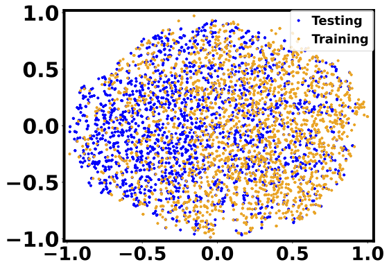
(d) $d_{W}=0.15$

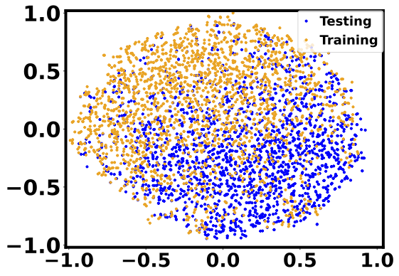
(e) $d_{W}=0.2$

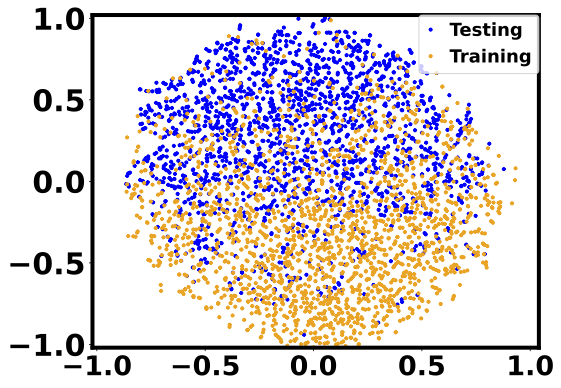
(f) $d_{W}=0.25$

Figure 4: Visualization of training-testing distribution discrepancy using t-SNE (Maaten and Hinton 2008). Blue and orange dots represent the testing and training samples, respectively.

Setup of Training

We consider using a neural network model as the ML model in LAAU and RL. In both LAAU and RL, we use fully-connected neural networks with 2 layers, each with 10 neurons. The neural network is trained by Adam optimizer with batch size as 10. We choose a learning rate of $5\times 10^{-3}$ for 50 epochs and a learning rate of $2.5\times 10^{-3}$ for the following 30 epochs. We run the training and testing experiments on a single CPU.

C.2 Details of Baselines

$\bullet$ Optimal Oracle (OPT): The optimal oracle knows the complete information $(\bm{c},\bm{B})$ for at the beginning of each episode and solves the problem in Eqn. (1).

$\bullet$ Equal Resource Allocation (Equal): The agent equally allocates the total resource capacity to $N$ jobs, i.e., each job receives $\frac{B}{N}$.

$\bullet$ Resource Allocation with Average Long-term Constraints (AVG-LT): AVG-LT minimizes the expected cost by relaxing the short-term capacity constraints in Eqn. (10) as $\mathrm{E}_{\mathcal{P}}\left[\sum_{t=1}^{N}x_{t}\right]\leq B$. Then, it uses the optimal Lagrangian multiplier for this relaxed problem as $\lambda_{t}$ for online allocation.

$\bullet$ Online Dual Gradient Descent (DGD (Balseiro, Lu, and Mirrokni 2020)): DGD, as one of the Dual Mirror Descent (DMD) algorithms, is designed to solve online constrained optimization with long-term constraints. It updates the Lagrangian multiplier in each step by gradient descent and then projecting the Lagrangian multiplier to the non-negative space. To make DGD better for OOBC, we slightly revise DGD on the basis of Algorithm 1 in (Balseiro, Lu, and Mirrokni 2020) by setting the allocation decision for job $N$ as $\min\left(b_{N},x_{\max}\right)$. The Lyapunov optimization technique (Neely 2010) also belongs to DGD.

$\bullet$ Online Multiplicative Weight (MW (Balseiro, Lu, and Mirrokni 2020)): Similar as DGD, MW is also a MDM method for solving online constrained optimization with long-term constraints. It also estimates the Lagrangian multiplier in an online style, but it updates the Lagrangian multiplier by multiplication (Arora, Hazan, and Kale 2012). Also, we revise MW to make it more suitable for OCO-SC in the same way as DGD.

$\bullet$ Reinforcement Learning (RL):RL is a machine learning algorithm based on offline data to learn the decision at each step. OOBC can be formulated as a reinforcement learning problem by viewing the remaining budget $\bm{b}_{t}$ and the parameter $c_{t}$ as states and the decision $x_{t}$ as the action. The reward function is the sum of the negative loss, i.e. $-\sum_{t=1}^{N}l(x_{t},c_{t})$. In RL, we use the neural network with the same depth and widths as LAAU, but output of the neural network in RL is directly the action and no optimization layer like (4) is used in RL.

For fair comparison, in all the baselines, if any decision results in capacity violation, we also apply projection to the decision to meet the total resource capacity constraint.

C.3 Settings of OOD Testing

The distribution used to generate synthetic training problem instances may be different from the true environment distribution, creating a distributional discrepancy and decreasing learning-based model performance (Goodfellow, Bengio, and Courville 2016). We measure the training-testing distributional difference in terms of the Wasserstein distance $d_{W}$. To create the distributional difference, we add i.i.d. Gaussian noise with different means and variances to the training data in the default setting.

We visualize in Fig. 4 the training-testing distributional differences using t-SNE (which converts high-dimensional distribution into a 2-dimensional one for visualization) (Maaten and Hinton 2008) under different Wasserstein distances. We can see that when $d_{W}=0.25$, the distributional difference is fairly large, with well separated testing and training samples.

C.4 Further Results

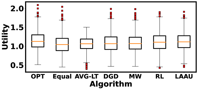
Figure 5: Distribution of Average utility (episode length $N=20$).

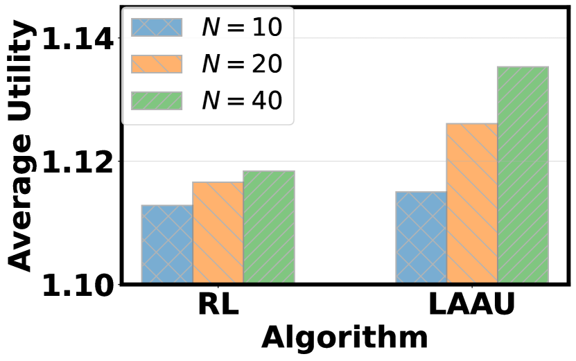
Figure 6: Average utility with different episode lengths.

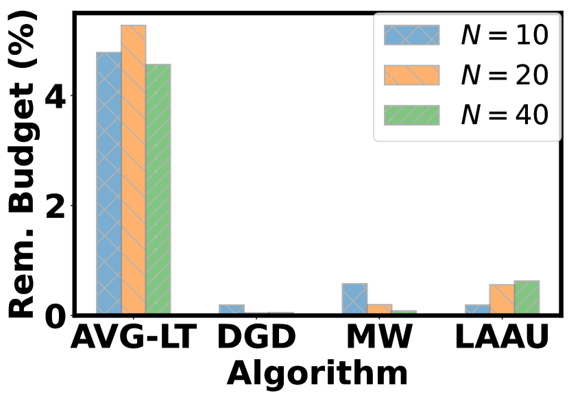
Figure 7: Average remaining budget

RL and LAAU with Different Lengths $N$

In Figure 7, we compare the average utilities of RL and LAAU in terms of different number of jobs $N$. We find that when $N$ is larger, LAAU outperforms RL more. This is because the unrolling architecture of LAAU exploits the knowledge from the optimization layers (4) and hence benefits generalization. When $N$ increases, LAAU uses more optimization layers while RL uses more neural layers, making the advantage of LAAU compared with RL become larger. This shows the benefit of the unrolling architecture in reducing generalization error.

Distribution of Average Utility

In Figure 7, we show the distribution of utility when the episode length $N=20$. For each algorithm, we give the median, 25 and 75 percentile, maximum and minimum utility, and the outliers. The results show that LAAU has the best median and 25% percentile tail utility among all the other baselines except OPT. In addition, the baseline algorithms do not have a substantial advantage over LAAU in terms of the minimum utility.

Remaining Resource

We show in Fig. 7 the average remaining resources for different algorithms. OPT and Equal use up all the resources and hence is not shown. We can find that the remaining resource of AVG-LT is the highest because the Lagrangian multiplier of AVG-LT is constant and cannot be updated according to the input parameters and remaining resource budgets online. The algorithms based on DMD, i.e. DGD and MW, both have low remaining budgets. This is because they aim to converge to the optimal Lagrangian multiplier that optimizes the dual problem of the original problem, which can guarantee a low complementary slackness (sum of the products of the Lagrangian multiplier and the remaining resource), as proved in Proposition 5 of (Balseiro, Lu, and Mirrokni 2020). LAAU, albeit having a slightly higher remaining resource than DGD and MW when $N$ is large, still achieves a sufficiently low remaining resource (less than 1%). The reason for remaining resources is the per-step allocation constraint. Importantly, LAAU has higher average utility with slightly lower utilized resource capacities than DMD, which further demonstrates the advantages of LAAU.

Appendix D Proofs of Conclusions in Section 5

In this section ,we first drive the gradients in Proposition 5.1 and then prove the conditions for differentiable KKT in Proposition 5.2. First, the notations are given as follows.
Notations: The gradient of $\bm{x}\in\mathbb{R}^{d}$ regarding $\bm{y}\in\mathbb{R}^{q}$ is denoted as $\bigtriangledown_{\bm{y}}\bm{x}\in\mathbb{R}^{d\times q}$. $\bigtriangledown_{\bm{x}}f(\bm{x})\in\mathbb{R}^{d}$ is the gradient of the function $f(\bm{x})$ regarding $\bm{x}\in\mathbb{R}^{d}$. $\bigtriangledown_{\bm{x}\bm{x}}f(\bm{x})\in\mathbb{R}^{d\times d}$ is the Hessian matrix of $f(\bm{x})$. $\mathrm{E}[\,\cdot\,]$ means taking expectation. $\mathrm{diag}(\bm{x})$ returns a diagonal matrix with the diagonal elements from $\bm{x}$.

D.1 Proof of Proposition 5.1

Proof.

To derive the gradients of the optimization layer, we start from the KKT conditions of the corresponding constrained optimization (4) as below.

$$\left\{\begin{matrix}\bigtriangledown_{x_{t}}l\left(x_{t},c_{t}\right)+\sum_{m=1}^{M}\left(\lambda_{m,t}+\mu_{m,t}\right)\bigtriangledown_{x_{t}}g_{m}\left(x_{t},c_{t}\right)=\bm{0}_{1\times d}\\ \mu_{t}\bigodot\left(\bm{g}\left(x_{t},c_{t}\right)-\bm{b}_{t}\right)=\bm{0}_{M}\\ \bm{g}\left(x_{t},c_{t}\right)\leq\bm{b}_{t},\mu_{t}\geq 0.\end{matrix}\right.,$$ (11)

where $\bigodot$ is the Hadamard product, $\mu_{t}\in\mathbb{R}^{M}$ is the optimal dual variable for the constrained optimization (4), the first equation is called stationarity, the second equation is called complementary slackness, and the two inequalities are primal and dual feasibility, respectively. Note that both the optimal primal variable $x_{t}$ and the optimal dual variable $\mu_{t}$ rely on the inputs of (4) including $\lambda_{t}$ and $\bm{b}_{t}$.

We first derive the gradient of $x_{t}$ with respect to $\lambda_{t}$. Taking gradient for both sides of the first two equations in (11) with respect to $\lambda_{t}$, we get

$$\begin{split}&\begin{bmatrix}\bigtriangledown_{x_{t}x_{t}}\!l\left(x_{t},c_{t}\right)+\sum_{m=1}^{M}\!\!\left(\lambda_{m,t}+\mu_{m,t}\right)\!\!\bigtriangledown_{x_{t}x_{t}}\!g_{m}\!\left(x_{t},c_{t}\right)&\left[\bigtriangledown_{x_{t}}\bm{g}\left(x_{t},c_{t}\right)\right]^{\top}\\ \left[\mu_{1,t}\left[\bigtriangledown_{x_{t}}g_{1}\left(x_{t},c_{t}\right)\right]^{\top},\cdots,\mu_{M,t}\!\left[\bigtriangledown_{x_{t}}g_{M}\left(x_{t},c_{t}\right)\right]^{\top}\right]^{\top}&\mathrm{diag}\left(\bm{g}\left(x_{t},c_{t}\right)-\bm{b}_{t}\right)\end{bmatrix}\begin{bmatrix}\bigtriangledown_{\lambda_{t}}x_{t}\\ \bigtriangledown_{\lambda_{t}}\mu_{t}\end{bmatrix}\\ &+\begin{bmatrix}\left[\bigtriangledown_{x_{t}}\bm{g}\left(x_{t},c_{t}\right)\right]^{\top}\\ \bm{0}_{M\times M}\end{bmatrix}=\bm{0}_{(d+M)\times M}.\end{split}$$ (12)

Denote the first matrix in Eqn. (12) as $\Delta$, and its four blocks are $\Delta_{11}=\bigtriangledown_{x_{t}x_{t}}\!l\left(x_{t},c_{t}\right)+\sum_{m=1}^{M}\!\!\left(\lambda_{m,t}+\mu_{m,t}\right)\!\!\bigtriangledown_{x_{t}x_{t}}\!\!g_{m}\!\left(x_{t},cf_{t}\right)$, $\Delta_{12}=\left[\bigtriangledown_{x_{t}}\bm{g}\left(x_{t},c_{t}\right)\right]^{\top}$, $\Delta_{21}=\left[\mu_{1,t}\!\left[\bigtriangledown_{x_{t}}g_{1}\left(x_{t},c_{t}\right)\right]^{\top},\cdots,\mu_{M,t}\!\left[\bigtriangledown_{x_{t}}g_{M}\left(x_{t},c_{t}\right)\right]^{\top}\right]^{\top}$ and $\Delta_{22}=\mathrm{diag}\left(\bm{g}\left(x_{t},c_{t}\right)-\bm{B}_{t}\right)$. Also, we denote the Schur-complement of $\Delta_{11}$ in the matrix $\Delta$ as $\mathrm{Sc}\left(\Delta,\Delta_{11}\right)=\Delta_{22}-\Delta_{21}\Delta^{-1}_{11}\Delta_{12}$. If $\mathrm{Sc}\left(\Delta,\Delta_{11}\right)$ is invertible (we give the conditions for this in Proposition 5.2), by block-wise matrix inverse, we can solve the gradient $\bigtriangledown_{\lambda_{t}}x_{t}$ as

$$\bigtriangledown_{\lambda_{t}}x_{t}=-\left(\Delta_{11}^{-1}+\Delta_{11}^{-1}\Delta_{12}\mathrm{Sc}\left(\Delta,\Delta_{11}\right)^{-1}\Delta_{21}\Delta_{11}^{-1}\right)\Delta_{12}.$$ (13)

Next, we drive the gradient of $x_{t}$ with respect to $\mathbf{b}_{t}$. Similarly, Taking gradient for both sides of the first two equations in (11) with respect to $\bm{b}_{t}$, we get

$$\begin{split}&\begin{bmatrix}\bigtriangledown_{x_{t}x_{t}}l\left(x_{t},c_{t}\right)+\sum_{m=1}^{M}\!\left(\lambda_{m,t}+\mu_{m,t}\right)\!\bigtriangledown_{x_{t}x_{t}}\!g_{m}\!\left(x_{t},c_{t}\right)&\left[\bigtriangledown_{x_{t}}\bm{g}\left(x_{t},c_{t}\right)\right]^{\top}\\ \left[\mu_{1,t}\!\left[\bigtriangledown_{x_{t}}g_{1}\left(x_{t},c_{t}\right)\right]^{\top},\cdots,\mu_{M,t}\!\left[\bigtriangledown_{x_{t}}g_{M}\left(x_{t},c_{t}\right)\right]^{\top}\right]^{\top}&\mathrm{diag}\left(\bm{g}\left(x_{t},c_{t}\right)-\bm{b}_{t}\right)\end{bmatrix}\begin{bmatrix}\bigtriangledown_{\bm{b}_{t}}x_{t}\\ \bigtriangledown_{\bm{b}_{t}}\mu_{t}\end{bmatrix}\\ &+\begin{bmatrix}\bm{0}_{d\times M}\\ -\mathrm{diag}(\mu_{t})\end{bmatrix}=\bm{0}_{(d+M)\times M}.\end{split}$$ (14)

Thus by solving Eqn.(14) with block-wise matrix inverse lemma, we have

$$\bigtriangledown_{\bm{b}_{t}}x_{t}=-\Delta_{11}^{-1}\Delta_{12}\mathrm{Sc}\left(\Delta,\Delta_{11}\right)^{-1}\mathrm{diag}(\mu_{t}).$$ (15)

∎

D.2 Proof of Proposition  5.2

Proof.

By the proof in Section D.1 to derive the gradients in Proposition 5.1, we can find that if $\Delta_{11}$ and its Schur-complement $\mathrm{Sc}(\Delta,\Delta_{11})$ are invertible and the norm of $\Delta_{12}$ and $\Delta_{21}$ is finite, then KKT based differentiation is viable.

First, if the norms of the constraint functions $\left\|\bigtriangledown_{x_{t}}g_{m}\left(x_{t},c_{t}\right)\right\|_{2}$ are bounded, then the norm of $\Delta_{12}$ and $\Delta_{21}$ is finite. Then, we give the condition that $\Delta_{11}$ is invertible. Since $\Delta_{11}$ is the Hessian matrix of the Lagrangian relaxed objective $l\left(x_{t},c_{t}\right)+\sum_{m=1}^{M}\!\!\left(\lambda_{m,t}+\mu_{m,t}\right)g_{m}\left(x_{t},\bm{c}_{t}\right)$, $\Delta_{11}$ is revertible only if it is positive definite. Given that $\lambda_{m,t}$ which is the output of machine learning model can be forced to be positive, we require that the loss function $l$ or any constraint function $g_{m},m=1,\cdots,M$ is strongly convex with respect to $x_{t}$, which guarantees that $\bigtriangledown_{x_{t},x_{t}}l\left(x_{t},c_{t}\right)$ or $\bigtriangledown_{x_{t},x_{t}}g_{m}\left(x_{t},\bm{c}_{t}\right)$ for any $m=1\dots,M$ is positive definite.

Finally, we prove the conditions can guarantee that $\mathrm{Sc}(\Delta,\Delta_{11})$ is invertible. Here for ease of notations, we omit the time step indices and the inputs of $g_{m}(x_{t},c_{t})$ and write $g_{m}(x_{t},c_{t})$ as $g_{m}$, $\mu_{m,t}$ as $\mu_{m}$. Remember that $\mathcal{A}$ is the index set of constraints that are activated. According to complementary slackness in KKT conditions (11), we know that if $m\notin\mathcal{A}$, i.e. $g_{m}<b_{m}$, then $\mu_{m}=0$. Here we denote $|\mathcal{A}|=M^{\prime}$, i.e. $M^{\prime}$ constraints are activated. To prove the condition, we reorder the $M$ constraints, change the indices of them and let $g_{m}<b_{m}$ and $\mu_{m}=0$ for $m=1\cdots,M-M^{\prime}$. Now $\mathcal{A}=\{M-M^{\prime}+1,\cdots,M\}$. From the conditions that $\mu_{m}\neq 0$ if $m\in\mathcal{A}$, we have $\mu_{m}>0$ and $g_{m}=b_{m}$ for $m=M-M^{\prime}+1,\cdots,M$. In other words, the first $M-M^{\prime}$ inequalities are un-activated and the last $M^{\prime}$ inequalities are activated. The Shur-complement of $\Delta_{11}$ can now be written as

$$\begin{split}&\mathrm{Sc}\left(\Delta,\Delta_{11}\right)\\ =&\begin{bmatrix}\mathrm{diag}(\left[\bm{g}-\bm{b}\right]_{1:M-M^{\prime}})&\bm{0}_{(M-M^{\prime})\times(M-M^{\prime})}\\ -\left[\Delta_{21}\right]_{M-M^{\prime}+1:M}\Delta_{11}^{-1}\left[\Delta_{12}\right]_{:,1:M-M^{\prime}}&-\left[\Delta_{21}\right]_{M-M^{\prime}+1:M}\Delta_{11}^{-1}\left[\Delta_{12}\right]_{:,M-M^{\prime}+1:M}\end{bmatrix}.\end{split}$$ (16)

where $\bm{X}_{a:b}$ denotes the sub-matrix concatenated by rows of matrix $\bm{X}$ with indices $a,a+1,\cdots,b$, $\bm{X}_{:,a:b}$ denotes the sub-matrix concatenated columns of matrix $\bm{X}$ with indices $a,a+1,\cdots,b$. By Block matrix determinant lemma, we have

$$\mathrm{det}\left(\mathrm{Sc}\left(\Delta,\Delta_{11}\right)\right)=\mathrm{det}\left(\mathrm{diag}(\left[\bm{g}-\bm{b}\right]_{1:M-M^{\prime}})\right)\mathrm{det}\left(-\left[\Delta_{21}\right]_{M-M^{\prime}+1:M}\Delta_{11}^{-1}\left[\Delta_{12}\right]_{:,M-M^{\prime}+1:M}\right).$$ (17)

We have $\mathrm{det}\left(\mathrm{diag}(\left[\bm{g}-\bm{b}\right]_{1:M-M^{\prime}})\right)\neq 0$ since $g_{m}<b_{m}$ for $m=1\cdots,M-M^{\prime}$. Now it remains to prove $\left[\Delta_{21}\right]_{M-M^{\prime}+1:M}\Delta_{11}^{-1}\left[\Delta_{12}\right]_{:,M-M^{\prime}+1:M}$ has full rank. To do that, we can rewrite the matrix as

$$\left[\Delta_{21}\right]_{M-M^{\prime}+1:M}\Delta_{11}^{-1}\left[\Delta_{12}\right]_{:,M-M^{\prime}+1:M}=\mathrm{diag}\left(\mu_{\mathrm{act}}\right)\bigtriangledown_{x_{t}}\!\!\bm{g}_{\mathrm{act}}\Delta_{11}^{-1}\bigtriangledown_{x_{t}}\!\!\bm{g}^{\top}_{\mathrm{act}},$$ (18)

where $\mu_{\mathrm{act}}=\left[\mu_{M-M^{\prime}+1},\cdots,\mu_{M}\right]$ is a non-zero vector according to the condition, and $\bigtriangledown_{x_{t}}\bm{g}_{\mathrm{act}}=\left[\bigtriangledown_{x_{t}}\bm{g}\right]_{M-M^{\prime}+1:M}$ is the gradient matrix regarding the activated constraint functions. By the condition that the gradients regarding the activated constraint functions are linear dependent and $d\geq M^{\prime}$, we have $\mathrm{rank}(\bigtriangledown_{x_{t}}\bm{g}_{\mathrm{act}})=M^{\prime}$. We have proved that $\Delta_{11}$ is invertible by our conditions, so we have $\mathrm{rank}(\Delta_{11}^{-1})=d$ and $\mathrm{rank}(\Delta_{11}^{-1/2})=d$ with $\mathrm{rank}(\Delta_{11}^{-1})=\mathrm{rank}(\Delta_{11}^{-1/2})\mathrm{rank}(\Delta_{11}^{-1/2})$. Since for a real matrix $\bm{X}$, $\mathrm{rank}(\bm{X}^{\top}\bm{X})=\mathrm{rank}(\bm{X})$, and a matrix and its Gram matrix have the same rank, we have

$$\mathrm{rank}\left(\bigtriangledown_{x_{t}}\bm{g}_{\mathrm{act}}\Delta_{11}^{-1}\bigtriangledown_{x_{t}}\bm{g}^{\top}_{\mathrm{act}}\right)=\mathrm{rank}\left(\bigtriangledown_{x_{t}}\bm{g}_{\mathrm{act}}\Delta_{11}^{-1/2}\right)=M^{\prime},$$ (19)

where the second equality holds due to Sylvester’s rank inequality such that $\mathrm{rank}\left(\bigtriangledown_{x_{t}}\bm{g}_{\mathrm{act}}\Delta_{11}^{-1/2}\right)\geq M^{\prime}$ and the fact that $\mathrm{rank}\left(\bigtriangledown_{x_{t}}\bm{g}_{\mathrm{act}}\Delta_{11}^{-1/2}\right)\leq\min\left(\mathrm{rank}\left(\bigtriangledown_{x_{t}}\bm{g}_{\mathrm{act}}\right),\mathrm{rank}\left(\Delta_{11}^{-1/2}\right)\right)=M^{\prime}$. Since $\mu_{\mathrm{act}}>0$, we have

$$\mathrm{det}\left(\mathrm{Sc}\left(\Delta,\Delta_{11}\right)\right)=\mathrm{det}\left(\mathrm{diag}(\left[\bm{g}-\bm{b}\right]_{1:M-M^{\prime}})\right)\mathrm{det}\left(\mathrm{diag}\left(\mu_{\mathrm{act}}\right)\right)\mathrm{det}\left(\bigtriangledown_{x_{t}}\bm{g}_{\mathrm{act}}\Delta_{11}^{-1}\bigtriangledown_{x_{t}}\bm{g}^{\top}_{\mathrm{act}}\right)>0,$$ (20)

Thus $\mathrm{Sc}\left(\Delta,\Delta_{11}\right)$ has full rank and is invertible, which completes the proof.

∎

Appendix E Proofs of Results in Section 6

E.1 Proof of Theorem 6.1

Lemma E.1 (Sensitivity of the total loss.).

If the ML model $f_{\theta}$ is Lipschitz continuous with respect to the resource capacity input $\bm{B}$ and parameter input $\bm{c}$ are bounded, and the conditions in Proposition 5.2 are satisfied, then the loss $L(\bm{h}_{\theta})$ is Lipschitz continuous with respect to the context sequence $\bm{c}$ and total budget $\bm{B}$, i.e.

$$L(\pi_{\theta},(\bm{c},\bm{B}))-L(\pi_{\theta},(\bm{c}^{\prime},\bm{B}^{\prime}))\leq\Gamma_{L,c}\omega_{c}+\Gamma_{L,b}\omega_{b},$$

where $\omega_{c}=\max_{\bm{c},\bm{c}^{\prime}\in\mathbb{C}}\left\|\bm{c}-\bm{c}^{\prime}\right\|$ is the size of the parameter space $\mathbb{C}$, $\omega_{b}=\max_{\bm{B},\bm{B}^{\prime}\in\mathbb{B}}\left\|\bm{B}-\bm{B}^{\prime}\right\|$ is the size of the resource capacity space $\mathbb{B}$, and $\Gamma_{L,c}$ and $\Gamma_{L,b}$ are bounded.

Proof.

We first bound the Lipschitz constants of the optimization layer $p(c_{t},\lambda_{t},\bm{b}_{t})$ with respect to $\lambda_{t}$,$\bm{b}_{t}$, and $c_{t}$. Taking $l_{2}$-norm for both sides of Eqn. (13) and using triangle inequality, we have

$$\begin{split}\left\|\bigtriangledown_{\lambda_{t}}\!x_{t}\right\|_{2}&\leq\left\|\Delta_{11}^{-1}\Delta_{12}\right\|_{2}+\left\|\Delta_{11}^{-1}\Delta_{12}\mathrm{Sc}\left(\Delta,\Delta_{11}\right)^{-1}\Delta_{21}\Delta_{11}^{-1}\Delta_{12}\right\|_{2}\\ &\leq\left\|\Delta_{11}^{-1}\Delta_{12}\right\|_{2}+\left\|\Delta_{11}^{-1}\Delta_{12}\right\|_{2}\left\|\mathrm{Sc}\left(\Delta,\Delta_{11}\right)^{-1}\right\|_{2}\left\|\Delta_{21}\right\|_{2}\left\|\Delta_{11}^{-1}\Delta_{12}\right\|_{2},\end{split}$$ (21)

where the second inequality holds because any induced operator norm is sub-multiplicative.

Denote the Lipschitz constants for $l$ and $g_{m}$ for any $m=1,\cdots,M$ are $\Gamma_{l}$ and $\Gamma_{g}$ respectively. Then we have $\left\|\bigtriangledown_{x_{t}}l\left(x_{t},c_{t}\right)\right\|_{2}\leq\Gamma_{l,x}$ and $\left\|\bigtriangledown_{x_{t}}g_{m}\left(x_{t},c_{t}\right)\right\|_{2}\leq\Gamma_{g,x}$ for any $m=1,\cdots,M$. Thus we have $\left\|\Delta_{12}\right\|_{F}=\left\|\bigtriangledown_{x_{t}}\!\bm{g}\left(x_{t},\bm{c}_{t}\right)\right\|_{F}\leq\sqrt{M}\Gamma_{g,x}$ and $\left\|\Delta_{21}\right\|_{F}\leq\bar{\mu}\sqrt{M}\Gamma_{g,x}$ where $\bar{\mu}$ is the largest dual variable for any $m=1,\cdots M$ and $t=1,\cdots,N$. Also, we have the norm of Hessian matrices bounded as $0\leq\breve{\rho}_{l,x,x}\leq\left\|\bigtriangledown_{x_{t}x_{t}}\!l\left(x_{t},c_{t}\right)\right\|_{2}\leq\bar{\rho}_{l,x,x}$ and $0\leq\breve{\rho}_{g,x,x}\leq\left\|\bigtriangledown_{x_{t}x_{t}}g_{m}\left(x_{t},\bm{c}_{t}\right)\right\|_{2}\leq\bar{\rho}_{g,x,x}$ by the convexity of $l$ and convexity of $g_{m}$. Since either $l$ or one of $g_{m},m=1,\cdots,M$ is strongly convex, the least singular value of $\Delta_{11}$ is larger than or equal to $\breve{\rho}_{l,g}=\min\left\{\breve{\rho}_{l,x,x},\breve{\lambda}\breve{\rho}_{g,x,x}\right\}$ where $\breve{\lambda}$ is the lower bounds of $\lambda_{m,t}$. Thus, we have $\left\|\Delta_{11}^{-1}\right\|_{2}\leq\frac{1}{\breve{\rho}_{l,g}}$. Thus we have $\left\|\Delta_{11}^{-1}\Delta_{12}\right\|_{2}\leq\left\|\Delta_{11}^{-1}\right\|_{2}\left\|\Delta_{12}\right\|_{F}\leq\sqrt{M}\frac{\Gamma_{g,x}}{\breve{\rho}_{l,g}}$.

If the conditions in Proposition 5.2 are satisfied, by the proof of Proposition 5.2, $\mathrm{Sc}\left(\Delta,\Delta_{11}\right)^{-1}$ has full rank and $\left\|\mathrm{Sc}\left(\Delta,\Delta_{11}\right)^{-1}\right\|_{2}$ is upper bounded. By Eqn. (16), the smallest singular value of $\mathrm{Sc}\left(\Delta,\Delta_{11}\right)^{-1}$ is expressed as

$$\sigma_{\min}\left(\mathrm{Sc}\left(\Delta,\Delta_{11}\right)\right)=\min\left\{\min\left\{\left|g_{m}-b_{m}\right|,m\notin\mathcal{A}\right\},\sigma_{\min}\left(\left[\Delta_{21}\right]_{\mathcal{A}}\Delta_{11}^{-1}\left[\Delta_{12}\right]_{\mathcal{A}}\right)\right\},$$ (22)

where $\sigma_{\min}\left(\cdot\right)$ returns the smallest singular value of a matrix and $\bm{X}_{\mathcal{A}}$ is a sub-matrix of $\bm{X}$ with indices in $\mathcal{A}$. For ease of notation, we denote $\sigma_{p,\lambda}=\sigma_{\min}\left(\left[\Delta_{21}\right]_{\mathcal{A}}\Delta_{11}^{-1}\left[\Delta_{12}\right]_{\mathcal{A}}\right)$. Also, we denote $\mathrm{gap}(\bm{g},\bm{b})=\min\left\{\left|g_{m}-b_{m}\right|,m=1,\cdots,M^{\prime}\right\}$. Then, we have

$$\left\|\mathrm{Sc}^{-1}\left(\Delta,\Delta_{11}\right)\right\|_{2}=\sigma^{-1}_{\min}\left(\mathrm{Sc}\left(\Delta,\Delta_{11}\right)\right)=1/\min\left\{\mathrm{gap}(\bm{g},\bm{b}),\sigma_{p,\lambda}\right\}.$$ (23)

Combining with inequality (21), we have

$$\left\|\bigtriangledown_{\lambda_{t}}\!x_{t}\right\|_{2}\leq\sqrt{M}\frac{\Gamma_{g,x}}{\breve{\rho}_{l,g}}+\frac{M^{3/2}\bar{\mu}\Gamma_{g,x}^{3}}{\breve{\rho}_{l,g}^{2}\min\left\{d(\bm{g},\bm{b}),\sigma_{p,\lambda}\right\}}.$$ (24)

Similarly for the gradient of $p$ with respect to $\bm{b}_{t}$, And the corresponding bound is

$$\begin{split}\left\|\bigtriangledown_{\bm{b}_{t}}x_{t}\right\|_{2}&\leq\left\|\Delta_{11}^{-1}\Delta_{12}\right\|_{2}\left\|\mathrm{Sc}\left(\Delta,\Delta_{11}\right)^{-1}\right\|_{2}\left\|\mathrm{diag}(\mu_{t})\right\|_{2}\\ &\leq\frac{\sqrt{M}\Gamma_{g,x}\bar{\mu}}{\breve{\rho}_{l,g}\min\left\{d(\bm{g},\bm{b}),\sigma_{p,\lambda}\right\}}.\end{split}$$ (25)

And the gradient of $p$ with respect to $c_{t}$ can also be derived by KKT as

$$\begin{split}&\bigtriangledown_{c_{t}}\bm{x}_{t}=\Delta_{11}^{-1}\Delta_{12}\mathrm{Sc}\left(\Delta,\Delta_{11}\right)^{-1}\mathrm{diag}(\mu_{t})\bigtriangledown_{c_{t}}\bm{g}(x_{t},c_{t})\\ &-\!\left(\Delta_{11}^{-1}+\!\Delta_{11}^{-1}\Delta_{12}\mathrm{Sc}\left(\Delta,\Delta_{11}\right)^{-1}\!\!\Delta_{21}\Delta_{11}^{-1}\right)\!\!\left(\!\bigtriangledown_{x_{t}c_{t}}l(x_{t},c_{t})+\!\!\sum_{m=1}^{M}\left(\lambda_{m,t}+\mu_{m,t}\right)\bigtriangledown_{x_{t}c_{t}}g_{m}\left(x_{t},\bm{c}_{t}\!\right)\right).\end{split}$$ (26)

And the corresponding bound is

$$\begin{split}&\left\|\bigtriangledown_{c_{t}}\bm{x}_{t}\right\|_{2}\\ \leq&\left\|\Delta_{11}^{-1}+\Delta_{11}^{-1}\Delta_{12}\mathrm{Sc}\left(\Delta,\Delta_{11}\right)^{-1}\Delta_{21}\Delta_{11}^{-1}\right\|_{2}\left(\bar{\rho}_{l,x,c}+M(\bar{\lambda}+\bar{\mu})\bar{\rho}_{g,x,c}\right)\\ &+\left\|\Delta_{11}^{-1}\Delta_{12}\mathrm{Sc}\left(\Delta,\Delta_{11}\right)^{-1}\mathrm{diag}(\mu_{t})\bigtriangledown_{c_{t}}\bm{g}(x_{t},c_{t})\right\|_{2}\\ \leq&\frac{\bar{\rho}_{l,x,c}+M(\bar{\lambda}+\bar{\mu})\bar{\rho}_{g,x,c}}{\breve{\rho}_{l,g}}+\frac{Mq^{2}_{g,x}\bar{\mu}\bar{\rho}_{l,x,c}+M^{2}q^{2}_{g,x}(\bar{\mu}\bar{\lambda}+\bar{\mu}^{2})\bar{\rho}_{g,x,c}}{\breve{\rho}^{2}_{l,g}\min\left\{d(\bm{g},\bm{b}),\sigma_{p,\lambda}\right\}}+\frac{M\Gamma_{g,x}\bar{\mu}\Gamma_{g,c}}{\breve{\rho}_{l,g}\min\left\{d(\bm{g},\bm{b}),\sigma_{p,\lambda}\right\}},\end{split}$$ (27)

where the first inequality holds by triangle inequality and the assumptions that $\left\|\bigtriangledown_{x_{t}c_{t}}l(x_{t},c_{t})\right\|\leq\bar{\rho}_{l,x,c}$, $\left\|\bigtriangledown_{x_{t}c_{t}}g_{m}\left(x_{t},\bm{c}_{t}\right)\right\|\leq\bar{\rho}_{g,x,c}$ and $\lambda_{m,t}\leq\bar{\lambda},\mu_{m,t}\leq\bar{\mu}$.

Therefore, we prove that the Lipschitz constants of the optimization layer is bounded and we denote the upper bounds of $\left\|\bigtriangledown_{\lambda_{t}}\!x_{t}\right\|_{2}$, $\left\|\bigtriangledown_{\bm{b}_{t}}\!x_{t}\right\|_{2}$, and $\left\|\bigtriangledown_{\bm{c}_{t}}\!x_{t}\right\|_{2}$ as $\Gamma_{p,\lambda},\Gamma_{p,b}$ and $\Gamma_{p,c}$, respectively.

Next we prove that the sensitivity of the total loss are bounded. Let $x_{j,t},c_{j,t},\lambda_{j,t},\bm{b}_{j,t}$ be the values flowing through our recurrent architectures for the sample $(\bm{c}_{j},\bm{B}_{j})$ while let $x^{\prime}_{j,t},c^{\prime}_{j,t},\lambda^{\prime}_{j,t},\bm{b}^{\prime}_{j,t}$ be the values for $(\bm{c}^{\prime}_{j},\bm{B}^{\prime}_{j})$. Let $\omega_{c}=\max_{\bm{c},\bm{c}^{\prime}\in\mathbb{C}}\left\|\bm{c}-\bm{c}^{\prime}\right\|$ is the size of the parameter space $\mathbb{C}$, $\omega_{b}=\max_{\bm{B},\bm{B}^{\prime}\in\mathbb{B}}\left\|\bm{B}-\bm{B}^{\prime}\right\|$ is the size of the resource capacity space $\mathbb{B}$. By Lipschitz continuity of the optimization layer, we have

$$\begin{split}&L(\pi_{\theta},(\bm{c},\bm{B}))-L(\pi_{\theta},(\bm{c}^{\prime},\bm{B}^{\prime}))\\ =&\sum_{t=1}^{N}l(x_{j,t},c_{j,t})-l(x^{\prime}_{j,t},c^{\prime}_{j,t})\\ \leq&N\Gamma_{l,c}\omega_{c}+\Gamma_{l,x}\sum_{t=1}^{N}\left\|p(c_{j,t},\lambda_{j,t},\bm{b}_{j,t})-p(c^{\prime}_{j,t},\lambda^{\prime}_{j,t},\bm{b}^{\prime}_{j,t})\right\|\\ \leq&N\Gamma_{l,c}\omega_{c}+\Gamma_{l,x}\sum_{t=1}^{N}\left\|p(c_{j,t},\lambda_{j,t},\bm{b}_{j,t})-p(c^{\prime}_{j,t},\lambda_{j,t},\bm{b}_{j,t})\right\|\\ &+\left\|p(c^{\prime}_{j,t},\lambda_{j,t},\bm{b}_{j,t})-p(c^{\prime}_{j,t},\lambda^{\prime}_{j,t},\bm{b}_{j,t})\right\|+\left\|p(c^{\prime}_{j,t},\lambda^{\prime}_{j,t},\bm{b}_{t})-p(c^{\prime}_{j,t},\lambda^{\prime}_{j,t},\bm{b}^{\prime}_{j,t})\right\|\\ \leq&N\Gamma_{l,c}\omega_{c}+N\Gamma_{l,x}\Gamma_{p,c}\omega_{c}+\Gamma_{l,x}\Gamma_{p,\lambda}\sum_{t=1}^{N}\left\|\lambda_{j,t}-\lambda^{\prime}_{j,t}\right\|+\Gamma_{l,x}\Gamma_{p,b}\sum_{t=1}^{N}\left\|\bm{b}_{j,t}-\bm{b}^{\prime}_{j,t}\right\|\end{split}$$ (28)

If the Lipschitz constant of the neural network is $\Gamma_{f}$, we have

$$\left\|\lambda_{j,t}-\lambda^{\prime}_{j,t}\right\|\leq\Gamma_{f,b}\left\|\bm{b}_{t}-\bm{b}^{\prime}_{t}\right\|+\Gamma_{f,c}\omega_{c}.$$ (29)

By the expression of the remaining budget in Line 4 of Algorithm 1 and Lipchitz continuity of each layer, we have

$$\begin{split}\left\|\bm{b}_{j,t}-\bm{b}^{\prime}_{j,t}\right\|&\leq\left\|\bm{b}_{j,{t-1}}-\bm{b}^{\prime}_{j,{t-1}}\right\|+\left\|\bm{g}(x_{t-1},c_{t-1})-\bm{g}(x^{\prime}_{t-1},c^{\prime}_{t-1})\right\|\\ &\leq\left\|\bm{b}_{j,{t-1}}-\bm{b}^{\prime}_{j,{t-1}}\right\|+\Gamma_{g,x}\left\|x_{t-1}-x^{\prime}_{t-1}\right\|+\Gamma_{g,c}\omega_{c}\\ &\leq\left(1+\Gamma_{g,x}\Gamma_{p,b}\right)\left\|\bm{b}_{j,{t-1}}-\bm{b}^{\prime}_{j,{t-1}}\right\|+\Gamma_{g,x}\Gamma_{p,\lambda}\left\|\lambda_{t-1}-\lambda^{\prime}_{t-1}\right\|+\left(1+\Gamma_{p,c}\right)\omega_{c}\\ &\leq\left(1+\Gamma_{g,x}\Gamma_{p,b}+\Gamma_{g,x}\Gamma_{p,\lambda}\Gamma_{f,b}\right)\left\|\bm{b}_{j,{t-1}}-\bm{b}^{\prime}_{j,{t-1}}\right\|+\left(1+\Gamma_{p,c}+\Gamma_{g,x}\Gamma_{p,\lambda}\Gamma_{f,c}\right)\omega_{c}.\end{split}$$ (30)

By performing induction based on recurrent inequality (30), we have

$$\begin{split}&\left\|\bm{b}_{j,t}-\bm{b}^{\prime}_{j,t}\right\|\leq\left(1+\Gamma_{g,x}\Gamma_{p,b}+\Gamma_{g,x}\Gamma_{p,\lambda}\Gamma_{f,b}\right)^{t-1}\omega_{b}+\\ &\qquad\frac{\left(1+\Gamma_{p,c}+\Gamma_{g,x}\Gamma_{p,\lambda}\Gamma_{f,c}\right)\left(\left(1+\Gamma_{g,x}\Gamma_{p,b}+\Gamma_{g,x}\Gamma_{p,\lambda}\Gamma_{f,b}\right)^{t-1}-1\right)}{\Gamma_{g,x}\Gamma_{p,b}+\Gamma_{g,x}\Gamma_{p,\lambda}\Gamma_{f,b}}\omega_{c}.\end{split}$$ (31)

Combining with (29), we have

$$\begin{split}&\left\|\lambda_{j,t}-\lambda^{\prime}_{j,t}\right\|\leq\Gamma_{f,b}\left(1+\Gamma_{g,x}\Gamma_{p,b}+\Gamma_{g,x}\Gamma_{p,\lambda}\Gamma_{f,b}\right)^{t-1}\omega_{b}\\ &\qquad+\left(\Gamma_{p,b}\frac{\left(1+\Gamma_{p,c}+\Gamma_{g,x}\Gamma_{p,\lambda}\Gamma_{f,c}\right)\left(\left(1+\Gamma_{g,x}\Gamma_{p,b}+\Gamma_{g,x}\Gamma_{p,\lambda}\Gamma_{f,b}\right)^{t-1}-1\right)}{\Gamma_{g,x}\Gamma_{p,b}+\Gamma_{g,x}\Gamma_{p,\lambda}\Gamma_{f,b}}+\Gamma_{f,c}\right)\omega_{c}.\end{split}$$ (32)

Therefore, the loss difference in Eqn.(28) can be bounded as

$$\begin{split}&L(\pi_{\theta},(\bm{c},\bm{B}))-L(\pi_{\theta},(\bm{c}^{\prime},\bm{B}^{\prime}))\\ \leq&N\Gamma_{l,c}\omega_{c}+N\Gamma_{l,x}\Gamma_{p,c}\omega_{c}+\Gamma_{l,x}\Gamma_{p,\lambda}\sum_{t=1}^{N}\left\|\lambda_{j,t}-\lambda^{\prime}_{j,t}\right\|+\Gamma_{l,x}\Gamma_{p,b}\sum_{t=1}^{N}\left\|\bm{b}_{j,t}-\bm{b}^{\prime}_{j,t}\right\|\\ \leq&\omega_{c}\left(\frac{\Gamma_{l,x}(\Gamma_{p,\lambda}+1)N\Gamma_{p,b}\left(1+\Gamma_{p,c}+\Gamma_{g,x}\Gamma_{p,\lambda}\Gamma_{f,c}\right)\left(\left(1+\Gamma_{g,x}\Gamma_{p,b}+\Gamma_{g,x}\Gamma_{p,\lambda}\Gamma_{f,b}\right)^{t-1}-1\right)}{\Gamma_{g,x}\Gamma_{p,b}+\Gamma_{g,x}\Gamma_{p,\lambda}\Gamma_{f,b}}\right.\\ &\left.+N\Gamma_{l,c}+N\Gamma_{l,x}\Gamma_{p,c}+\Gamma_{l,x}\Gamma_{p,\lambda}N\Gamma_{f,c}\right)\\ &+\omega_{b}\Gamma_{l,x}\left(N\Gamma_{l,x}\Gamma_{p,\lambda}\Gamma_{f,b}+N\Gamma_{p,b}\right)\left(1+\Gamma_{g,x}\Gamma_{p,b}+\Gamma_{g,x}\Gamma_{p,\lambda}\Gamma_{f,b}\right)^{t-1}\\ \leq&\Gamma_{L,c}\omega_{c}+\Gamma_{L,b}\omega_{b}.\end{split}$$ (33)

∎

Proof of Theorem 6.1

Proof.

If Lemma E.1 holds, we can use the generalization theorem for Rademacher complexity (Bartlett and Mendelson 2002; Attias, Kontorovich, and Mansour 2019) to bound the expected loss, which states that for any $\theta\in\Theta$, with probability at least $1-\delta,\delta\in(0,1)$,

$$\begin{split}&\mathrm{E}\left[L(\bm{h}_{\theta},\bm{c})\right]\\ \leq&L\left(\bm{h}_{\theta},S\right)+2R_{n}(L\circ\mathbb{H})+\left(\Gamma_{L,c}\omega_{c}\!+\!\Gamma_{L,b}\omega_{b}\right)\!\sqrt{\frac{\ln(1/\delta)}{n}}.\end{split}$$ (34)

For the learned weight $\hat{\theta}$, we have with probability at least $1-\delta,\delta\in(0,1)$,

$$\begin{split}L\left(\bm{h}_{\hat{\theta}},S\right)&=L\left(\bm{h}_{\hat{\theta}},S\right)-L\left(\bm{h}_{\hat{\theta}^{*}},S\right)+L\left(\bm{h}_{\hat{\theta}^{*}},S\right)\\ &\leq\mathcal{E}\left(\bm{h}_{\hat{\theta}},S\right)+L\left(\bm{h}_{\theta^{*}},S\right)\\ &\leq\mathcal{E}\left(\bm{h}_{\hat{\theta}},S\right)+\mathrm{E}\left[L(\bm{h}_{\theta^{*}})\right]+2R_{n}(L\circ\mathbb{H})\\ &+\left(\Gamma_{L,c}\omega_{c}+\Gamma_{L,b}\omega_{b}\right)\sqrt{\frac{\ln(1/\delta)}{n}},\end{split}$$ (35)

where the first inequality holds because $\hat{\theta}^{*}$ minimizes the empirical loss $L\left(\bm{h}_{\hat{\theta}^{*}},S\right)$, and the second inequality holds by applying the generalization bound (34) to $L\left(\bm{h}_{\hat{\theta}^{*}},S\right)$. Combining Eqn. (34) and Eqn. (35) and applying union bound, we get the bound of expected loss in Theorem 6.1. ∎

E.2 Proof of Proposition 6.2

Definition 2 (Rademacher Complexity).

Let $\mathbb{H}=\left\{\bm{h}:\mathbb{B}\times\mathbb{C}\rightarrow\mathbb{X}\right\}$, where $\mathbb{B},\mathbb{C}$, and $\mathbb{X}$ are the spaces of $\bm{B},\bm{c}$, and $\bm{x}=[x_{1},\cdots,x_{N}]^{\top}$ respectively, be the function space of online optimizer and denote the space of the total loss as $L\circ\mathbb{H}=\left\{L(\bm{h}),\bm{h}\in\mathbb{H}\right\}$. Given the dataset $S=\left\{\left(\bm{c}_{1},\bm{B}_{1}\right),\cdots,\left(\bm{c}_{n},\bm{B}_{n}\right)\right\}$, the Rademacher complexity regarding the space of total loss is

$$R_{n}(L\circ\mathbb{H})=\mathrm{E}_{S}\mathrm{E}_{\nu}\left[\sup_{\bm{h}\in\mathbb{H}}\left(\frac{1}{n}\sum_{i=1}^{n}\nu_{i}L\left(\bm{h}(\bm{B}_{i},\bm{c}_{i})\right)\right)\right],$$

where $\nu_{1},\cdots,\nu_{n}$ are independently drawn from Rademacher distribution.

Proof of Proposition 6.2

Proof.

We consider two concrete examples for the ML model — linear and neural network models — used in our unrolled architecture shown in Fig. 1. We start with a linear model to substantiate the ML model in LAAU. Specifically, we have

$$f_{\theta}(\bm{v})=\theta^{\top}\phi(\bm{v})$$ (36)

where $\theta\in\Theta=\left\{\theta\in\mathbb{R}^{M\times q}\mid,\left\|\theta\right\|_{2}\leq Z\right\}$ is the weight to be learned, $\bm{v}=[\bm{b}_{t}^{\top},c_{t},\bar{t}]^{\top}$, $\phi:\mathbb{B}\times\mathbb{C}\times\mathbb{R}^{1}\rightarrow\mathbb{R}^{q}$ is a determinant feature mapping function which can be a manually-designed kernel or a pre-trained neural network.

According to our architecture in Fig. 1, the final online optimizer $\bm{h}$ is a composition of the optimizer $p$ and the ML model, i.e. $\bm{h}=p\circ\bm{f}_{\theta}$ where $\bm{f}_{\theta}=[f_{\theta}(\bm{b}_{1},c_{1}),\cdots,f_{\theta}(\bm{b}_{t},c_{t})]$ and $p$ is applied to each entry of $\bm{f}_{\theta}$. By (28), (29), and (30), for two different outputs $\lambda_{1}$ and $\lambda_{1}^{\prime}$ of the neural network for $t=1$ and the corresponding action $x_{t}$, $x_{t}^{\prime}$, we have

$$l(x_{t},c_{t})-l(x_{t}^{\prime},c_{t})\leq\Upsilon_{t}\|\lambda_{1}-\lambda_{1}^{\prime}\|,$$ (37)

where $\Upsilon_{t}=\Gamma_{l,x}\left(\Gamma_{p,\lambda}\Gamma_{f,b}+\Gamma_{l,x}\Gamma_{p,b}\right)\left(1+\Gamma_{g,x}\Gamma_{p,b}+\Gamma_{g,x}\Gamma_{p,\lambda}\Gamma_{f,b}\right)^{t-2}\Gamma_{g,x}\Gamma_{p,\lambda}$. According to the contraction lemma of Rademacher complexity in (Maurer 2016), we have

$$R_{n}(L\circ\mathbb{H})\leq N\sum_{t=1}^{N}\Upsilon_{t}\sum_{m=1}^{M}R_{n}(\mathbb{F}_{1,m}),$$ (38)

where $\mathbb{F}_{1,m}=\left\{\bm{f}_{\theta,1,m}:\mathbb{B}\times\mathbb{C}\rightarrow\Lambda^{1}\right\}$ is the function domain regarding the $m$th dimension of $\lambda_{t}$ output by the linear ML model.

Now we derive the Rademacher complexity of the ML model spaces $\mathbb{F}_{1,m}$. Let $\bm{v}_{i,t}=[\bm{b}_{t,i}^{\top},c_{t,i},\bar{t}]^{\top},i=1,\cdots,n$. Assume that $\|\theta_{m}\|_{2}=Z_{m}$ According to the definition of empirical Radmacher complexity, we have

$$\begin{split}\hat{R}_{n}(\mathbb{F}_{1,m})&=\mathrm{E}_{\nu}\left[\sup_{\bm{f}_{\theta,t,m}\in\mathbb{F}_{1,m}}\left(\frac{1}{n}\sum_{i=1}^{n}\nu_{i}\bm{f}_{\theta,t,m}(\bm{B}_{i},\bm{c}_{i})\right)\right]\\ &=\mathrm{E}_{\nu}\left[\sup_{\bm{f}_{\theta,t,m}\in\mathbb{F}_{1,m}}\left(\frac{1}{n}\sum_{i=1}^{n}\nu_{i}\theta_{m}^{\top}\phi(\bm{v}_{i,t})\right)\right]\\ &=\frac{1}{n}\mathrm{E}_{\nu}\left[Z_{m}\left\|\sum_{i=1}^{n}\nu_{i}\phi(\bm{v}_{i,t})\right\|_{2}\right]\\ &\leq\frac{Z_{m}}{n}\sqrt{\mathrm{E}_{\nu}\left\|\sum_{i=1}^{n}\nu_{i}\phi(\bm{v}_{i,t})\right\|^{2}_{2}}\\ &=\frac{Z_{m}}{n}\sqrt{\sum_{i=1}^{n}\left\|\phi(\bm{v}_{i,t})\right\|^{2}_{2}}\leq\frac{Z_{m}W}{\sqrt{n}},\end{split}$$ (39)

where the third equality holds by Cauchy-Schwartz inequality, the first inequality holds by using Jensen’s inequality for the expectation, the forth equality holds since $\mathrm{E}\left[\nu_{i}\nu_{j}\right]=0$ when $i\neq j$ and the last inequality by the assumption that the norm of the feature mapping is at most $W$. Taking expectation over the dataset $S$, we have

$$R_{n}(\mathbb{F}_{1,m})=\mathrm{E}_{S}\left[\hat{R}_{n}(\mathbb{F}_{1,m})\right]\leq\frac{Z_{m}W}{\sqrt{n}}$$ (40)

Substituting inequality (40) into (38), since $\sum_{m=1}^{M}\|\theta_{m}\|_{2}\leq\sqrt{M}\|\theta\|,$we get the conclusion

$$R_{n}(L\circ\mathbb{H})\leq\sqrt{M}N^{2}\Upsilon_{N}\frac{ZW}{\sqrt{n}}$$ (41)

Next, We consider a fully neural network with $K$ hidden layers, each with the number of neurons no larger than $u$, which can be represented as

$$f_{\theta}(\bm{v})=\alpha_{K}\left(\theta_{K}\alpha_{K-1}\left(\theta_{K-1}\cdots\alpha_{1}\left(\theta_{1}\bm{v}\right)\right)\right),$$ (42)

where $\alpha_{k}(\cdot)$, for $k=1,\cdots,K$, is the activation function and $\theta_{k}$, for $k=1,\cdots,K$ is the weight for $k$-th layer.

Same as Eqn.(38), we have

$$R_{n}(L\circ\mathbb{H})\leq N\sum_{t=1}^{N}\Upsilon_{t}\sum_{m=1}^{M}R_{n}(\mathbb{F}_{1,m}),$$ (43)

where now $\mathbb{F}_{1,m}=\left\{\bm{f}_{\theta,t,m}:\mathbb{B}\times\mathbb{C}\rightarrow\Lambda^{1}\right\}$ is the function domain regarding the $m$-th dimension of $\lambda_{t}$ output by the neural network.

Denote $\bm{v}_{i,t}=[\bm{b}_{t,i}^{\top},c_{t,i},\bar{t}]^{\top},i=1,\cdots,n$ and $\bm{V}=[\bm{v}_{1,t};\bm{v}_{2,t},\cdots,\bm{v}_{n,t}]$. Denote the convering number of the space $\mathbb{F}_{1,m}$ as $\mathcal{N}(\mathbb{F}_{1,m},\epsilon,2)$ with respect to Scale $\epsilon$ and 2-norm which is defined in (Bartlett, Foster, and Telgarsky 2017) The Lipschitz constants of all the activation functions $\alpha_{k}$ are less than or equal to $\Gamma_{\alpha}$. Assume that the spectral norm of the weight in each layer satisfy $\left\|\theta_{k}\right\|_{2}\leq Z_{k},k=1,\cdots,K$. By Theorem 3.3 in (Bartlett, Foster, and Telgarsky 2017), the logarithm of the covering number $\mathcal{N}(\mathbb{F}_{1,m})$ of the space $\mathcal{N}(\mathbb{F}_{1,m},\epsilon,2)$ can be bounded as

$$\ln\mathcal{N}(\mathbb{F}_{1,m},\epsilon,2)\leq\frac{\|\bm{V}\|_{F}^{2}}{\epsilon^{2}}\left(\prod_{k=1}^{K}Z_{k}^{2}\Gamma_{\sigma}^{2}\right)\left(\sum_{k=1}^{K}\left(\frac{\left\|\left(\theta_{k}-\bar{\theta}_{k}\right)^{\top}\right\|^{2/3}_{2,1}}{Z_{k}^{2/3}}\right)\right)^{3},$$ (44)

where $\bar{\theta}_{k},k=1,\cdots,K$ are reference matrices with the same dimensions as $\theta_{k}$. We choose reference matrices with the same spectral norm bound as $\theta_{k}$, and simplify the logarithm of the covering number as

$$\ln\mathcal{N}(\mathbb{F}_{1,m},\epsilon,2)\leq\frac{4K^{3}u^{2}\|\bm{V}\|_{F}^{2}}{\epsilon^{2}}\left(\prod_{k=1}^{K}Z_{k}^{2}\Gamma_{\sigma}^{2}\right),$$ (45)

where the inequality holds because $\left\|\left(\theta_{k}-\bar{\theta}_{k}\right)^{\top}\right\|_{2,1}\leq\left\|\theta^{\top}_{k}\right\|_{2,1}+\left\|\bar{\theta}^{\top}_{k}\right\|_{2,1}\leq\sqrt{u}\left(\left\|\theta^{\top}_{k}\right\|_{F}+\left\|\bar{\theta}^{\top}_{k}\right\|_{F}\right)\leq u\left(\left\|\theta^{\top}_{k}\right\|_{2}+\left\|\bar{\theta}^{\top}_{k}\right\|_{2}\right)\leq 2uZ_{k}$.

Substituting (45) into Dudley entropy Integral, we have

$$\begin{split}\hat{R}_{n}(\mathbb{F}_{1,m})&\leq\inf_{\gamma>0}\left(\frac{4\gamma}{\sqrt{n}}+\frac{12}{n}\int_{\gamma}^{\sqrt{n}}\sqrt{\ln\mathcal{N}(\mathbb{F}_{1,m},\epsilon,2)}\mathrm{d}\epsilon\right)\\ &\leq\frac{24K^{3/2}u\|\bm{V}\|_{F}\Gamma_{\alpha}\prod_{k=1}^{K}Z_{k}}{n}\left(1+\ln\frac{n}{72K^{3/2}u\|\bm{V}\|^{1/2}\Gamma_{\alpha}\prod_{k=1}^{K}Z_{k}}\right)\\ &\leq\tilde{O}\left(\frac{K^{3/2}u\Gamma_{\alpha}(\beta_{b}+\beta_{c})\prod_{k=1}^{K}Z_{k}}{\sqrt{n}}\right),\end{split}$$ (46)

where the last inequality holds because $\|\bm{V}\|_{F}\leq\sqrt{n}\left(\beta_{b}+\beta_{c}\right)$ where $\beta_{b},\beta_{c}$ are the largest norm of budget $\bm{B}$ and parameter $c$, respectively.Taking expectation over the dataset $S$, we have

$$R_{n}(\mathbb{F}_{1,m})=\mathrm{E}_{S}\left[\hat{R}_{n}(\mathbb{F}_{1,m})\right]\leq\tilde{O}\left(\frac{K^{3/2}u\Gamma_{\alpha}(\beta_{b}+\beta_{c})\prod_{k=1}^{K}Z_{k}}{\sqrt{n}}\right).$$ (47)

Substituting inequality (47) into (43), we get the conclusion

$$R_{n}(L\circ\mathbb{H})\leq\sqrt{M}N^{2}\Upsilon_{N}\tilde{O}\left(\frac{K^{3/2}u\Gamma_{\alpha}(\beta_{b}+\beta_{c})\prod_{k=1}^{K}Z_{k}}{\sqrt{n}}\right).$$ (48)

∎

E.3 Proof of Proposition 6.3

Proof.

By Lemma 4.4 in (Bottou, Curtis, and Nocedal 2018), with the assumptions about training objective and instance sequence held, we have

$$\begin{split}&\mathrm{E}\left[L(h_{\hat{\theta}_{i+1}})-L(h_{\hat{\theta}_{i}})\right]\\ \leq&-\left(\iota-\frac{1}{2}\bar{\alpha}\Gamma_{\triangledown L,\theta}\left(\varpi_{V}+\iota_{G}^{2}\right)\right)\bar{\alpha}\left[\left\|\bigtriangledown_{\hat{\theta}}\mathrm{E}[L(h_{\hat{\theta}_{i}})]\right\|_{2}^{2}\right]+\frac{1}{2}\bar{\alpha}^{2}\Gamma_{\triangledown L,\theta}\varpi\\ \leq&-\iota\bar{\alpha}\varsigma\mathrm{E}\left[L(h_{\hat{\theta}_{i+1}})-L(h_{\theta^{*}})\right]+\frac{1}{2}\bar{\alpha}^{2}\Gamma_{\triangledown L,\theta}\varpi,\end{split}$$ (49)

where the expectation is taken over the randomness of the parameter sequence up to round $i$, the last inequality holds by the choice of $\bar{\alpha}$ and the assumption of Polyak-Lojasiewicz inequality. Subtracting $\mathrm{E}\left[L\left(h_{\theta^{*}}\right)\right]$ from both sides, we have

$$\begin{split}&\mathrm{E}\left[L(h_{\hat{\theta}_{i+1}})-L(h_{\theta^{*}})\right]\leq\left(1-\iota\bar{\alpha}\varsigma\right)\mathrm{E}\left[L(h_{\hat{\theta}_{i+1}})-L(h_{\theta^{*}})\right]+\frac{1}{2}\bar{\alpha}^{2}\Gamma_{\triangledown L,\theta}\varpi,\end{split}$$ (50)

and so

$$\begin{split}&\mathrm{E}\left[L(h_{\hat{\theta}_{i}})-L(h_{\theta^{*}})\right]-\frac{\bar{\alpha}\Gamma_{\triangledown L,\theta}\varpi}{2\iota\varsigma}\\ \leq&\left(1-\iota\bar{\alpha}\varsigma\right)\mathrm{E}\left[L(h_{\hat{\theta}_{i-1}})-L(h_{\theta^{*}})\right]+\frac{1}{2}\bar{\alpha}^{2}\Gamma_{\triangledown L,\theta}\varpi-\frac{\bar{\alpha}\Gamma_{\triangledown L,\theta}\varpi}{2\iota\varsigma}\\ =&\left(1-\iota\bar{\alpha}\varsigma\right)\left(\mathrm{E}\left[L(h_{\hat{\theta}_{i-1}})-L(h_{\theta^{*}})\right]-\frac{\bar{\alpha}\Gamma_{\triangledown L,\theta}\varpi}{2\iota\varsigma}\right).\end{split}$$ (51)

Thus, using inequality (51) recurrently, we have

$$\begin{split}\mathrm{E}\left[L(h_{\hat{\theta}_{i}})-L(h_{\theta^{*}})\right]-\frac{\bar{\alpha}\Gamma_{\triangledown L,\theta}\varpi}{2\iota\varsigma}\leq\left(1-\iota\bar{\alpha}\varsigma\right)^{i}\left(\mathrm{E}\left[L(h_{\hat{\theta}_{0}})-L(h_{\theta^{*}})\right]-\frac{\bar{\alpha}\Gamma_{\triangledown L,\theta}\varpi}{2\iota\varsigma}\right).\end{split}$$ (52)

Thus, we can bound the expected cost gap at round $i$ as

$$\begin{split}\mathrm{E}\left[L(h_{\hat{\theta}_{i}})-L(h_{\theta^{*}})\right]\leq\frac{\bar{\alpha}\Gamma_{\triangledown L,\theta}\varpi}{2\iota\varsigma}+O\left(\left(1-\iota\bar{\alpha}\varsigma\right)^{i}\right),\end{split}$$ (53)

where the expectation is taken over the parameter sequence at and before round $i$. ∎

References

- Adler and Öktem (2018) Adler, J.; and Öktem, O. 2018. Learned primal-dual reconstruction. IEEE transactions on medical imaging, 37(6): 1322–1332.
- Agrawal and Devanur (2014) Agrawal, S.; and Devanur, N. R. 2014. Fast algorithms for online stochastic convex programming. In Proceedings of the twenty-sixth annual ACM-SIAM symposium on Discrete algorithms, 1405–1424.
- Alomrani, Moravej, and Khalil (2021) Alomrani, M. A.; Moravej, R.; and Khalil, E. B. 2021. Deep Policies for Online Bipartite Matching: A Reinforcement Learning Approach. CoRR, abs/2109.10380.
- Arora, Hazan, and Kale (2012) Arora, S.; Hazan, E.; and Kale, S. 2012. The multiplicative weights update method: a meta-algorithm and applications. Theory of Computing, 8(1): 121–164.
- Attias, Kontorovich, and Mansour (2019) Attias, I.; Kontorovich, A.; and Mansour, Y. 2019. Improved generalization bounds for robust learning. In Algorithmic Learning Theory, 162–183.
- Azar et al. (2016) Azar, Y.; Buchbinder, N.; Chan, T. H.; Chen, S.; Cohen, I. R.; Gupta, A.; Huang, Z.; Kang, N.; Nagarajan, V.; Naor, J.; et al. 2016. Online algorithms for covering and packing problems with convex objectives. In 2016 IEEE 57th Annual Symposium on Foundations of Computer Science (FOCS), 148–157. IEEE.
- Balseiro, Lu, and Mirrokni (2020) Balseiro, S.; Lu, H.; and Mirrokni, V. 2020. Dual mirror descent for online allocation problems. In International Conference on Machine Learning, 613–628.
- Bartlett, Foster, and Telgarsky (2017) Bartlett, P.; Foster, D. J.; and Telgarsky, M. 2017. Spectrally-normalized margin bounds for neural networks. arXiv preprint arXiv:1706.08498.
- Bartlett and Mendelson (2002) Bartlett, P. L.; and Mendelson, S. 2002. Rademacher and Gaussian complexities: Risk bounds and structural results. Journal of Machine Learning Research, 3(Nov): 463–482.
- Bottou, Curtis, and Nocedal (2018) Bottou, L.; Curtis, F. E.; and Nocedal, J. 2018. Optimization methods for large-scale machine learning. Siam Review, 60(2): 223–311.
- Boyd, Boyd, and Vandenberghe (2004) Boyd, S.; Boyd, S. P.; and Vandenberghe, L. 2004. Convex optimization. Cambridge university press.
- Chen et al. (2018) Chen, R. T.; Rubanova, Y.; Bettencourt, J.; and Duvenaud, D. 2018. Neural ordinary differential equations. NeurIPS.
- Chen et al. (2021) Chen, T.; Chen, X.; Chen, W.; Heaton, H.; Liu, J.; Wang, Z.; and Yin, W. 2021. Learning to optimize: A primer and a benchmark. arXiv preprint arXiv:2103.12828.
- Dai et al. (2017) Dai, H.; Khalil, E. B.; Zhang, Y.; Dilkina, B.; and Song, L. 2017. Learning combinatorial optimization algorithms over graphs. In NIPS.
- Devanur and Hayes (2009) Devanur, N. R.; and Hayes, T. P. 2009. The adwords problem: online keyword matching with budgeted bidders under random permutations. In Proceedings of the 10th ACM conference on Electronic commerce, 71–78.
- Devanur et al. (2019) Devanur, N. R.; Jain, K.; Sivan, B.; and Wilkens, C. A. 2019. Near optimal online algorithms and fast approximation algorithms for resource allocation problems. Journal of the ACM (JACM), 66(1): 1–41.
- Du, Wu, and Huang (2019) Du, B.; Wu, C.; and Huang, Z. 2019. Learning resource allocation and pricing for cloud profit maximization. In Proceedings of the AAAI conference on artificial intelligence, volume 33, 7570–7577.
- El-Yaniv et al. (2001) El-Yaniv, R.; Fiat, A.; Karp, R. M.; and Turpin, G. 2001. Optimal search and one-way trading online algorithms. Algorithmica, 30(1): 101–139.
- Fan, Weber, and Barroso (2007) Fan, X.; Weber, W.-D.; and Barroso, L. A. 2007. Power provisioning for a warehouse-sized computer. In ISCA.
- Feldman et al. (2010) Feldman, J.; Henzinger, M.; Korula, N.; Mirrokni, V. S.; and Stein, C. 2010. Online stochastic packing applied to display ad allocation. In European Symposium on Algorithms, 182–194.
- Ghodsi et al. (2011) Ghodsi, A.; Zaharia, M.; Hindman, B.; Konwinski, A.; Shenker, S.; and Stoica, I. 2011. Dominant Resource Fairness: Fair Allocation of Multiple Resource Types. In Nsdi, volume 11, 24–24.
- Goodfellow, Bengio, and Courville (2016) Goodfellow, I.; Bengio, Y.; and Courville, A. 2016. Deep Learning. MIT Press. http://www.deeplearningbook.org.
- Gregor and LeCun (2010) Gregor, K.; and LeCun, Y. 2010. Learning fast approximations of sparse coding. In Proceedings of the 27th international conference on international conference on machine learning, 399–406.
- Haykin (2006) Haykin, S. 2006. Cognitive Radio: Brain-empowered Wireless Communications. IEEE J.Sel. A. Commun., 23(2): 201–220.
- He et al. (2013) He, J.; Xue, Z.; Wu, D.; Wu, D. O.; and Wen, Y. 2013. CBM: Online strategies on cost-aware buffer management for mobile video streaming. IEEE Transactions on Multimedia, 16(1): 242–252.
- Huang, Liu, and Hao (2014) Huang, L.; Liu, X.; and Hao, X. 2014. The Power of Online Learning in Stochastic Network Optimization. SIGMETRICS Perform. Eval. Rev., 42(1): 153–165.
- Hylland and Zeckhauser (1979) Hylland, A.; and Zeckhauser, R. 1979. The efficient allocation of individuals to positions. Journal of Political economy, 87(2): 293–314.
- Jiang, Li, and Zhang (2020) Jiang, J.; Li, X.; and Zhang, J. 2020. Online Stochastic Optimization with Wasserstein Based Non-stationarity. arXiv preprint arXiv:2012.06961.
- Joe-Wong et al. (2013) Joe-Wong, C.; Sen, S.; Lan, T.; and Chiang, M. 2013. Multi-resource Allocation: Fairness-efficiency Tradeoffs in a Unifying Framework. IEEE/ACM Trans. Netw., 21(6): 1785–1798.
- Kobler et al. (2020) Kobler, E.; Effland, A.; Kunisch, K.; and Pock, T. 2020. Total deep variation: A stable regularizer for inverse problems. arXiv preprint arXiv:2006.08789.
- Kolter, Duvenaud, and Johnson (2022) Kolter, Z.; Duvenaud, D.; and Johnson, M. 2022. Deep Implicit Layers. http://implicit-layers-tutorial.org/.
- Kong et al. (2019) Kong, W.; Liaw, C.; Mehta, A.; and Sivakumar, D. 2019. A New Dog Learns Old Tricks: RL Finds Classic Optimization Algorithms. In ICLR.
- Lan et al. (2010) Lan, T.; Kao, D.; Chiang, M.; and Sabharwal, A. 2010. An axiomatic theory of fairness in network resource allocation. In INFOCOM.
- Li and Malik (2017) Li, K.; and Malik, J. 2017. Learning to Optimize. In ICLR.
- Li et al. (2019) Li, Y.; Tofighi, M.; Monga, V.; and Eldar, Y. C. 2019. An algorithm unrolling approach to deep image deblurring. In ICASSP 2019-2019 IEEE International Conference on Acoustics, Speech and Signal Processing (ICASSP), 7675–7679. IEEE.
- Lin et al. (2022) Lin, Q.; Mo, Y.; Su, J.; and Chen, M. 2022. Competitive Online Optimization with Multiple Inventories: A Divide-and-Conquer Approach. Proceedings of the ACM on Measurement and Analysis of Computing Systems, 6(2): 1–28.
- Lin et al. (2019) Lin, Q.; Yi, H.; Pang, J.; Chen, M.; Wierman, A.; Honig, M.; and Xiao, Y. 2019. Competitive online optimization under inventory constraints. Proceedings of the ACM on Measurement and Analysis of Computing Systems, 3(1): 1–28.
- Liu et al. (2019) Liu, R.; Cheng, S.; Ma, L.; Fan, X.; and Luo, Z. 2019. Deep proximal unrolling: Algorithmic framework, convergence analysis and applications. IEEE Transactions on Image Processing, 28(10): 5013–5026.
- Liu et al. (2020) Liu, S.; Chen, P.-Y.; Kailkhura, B.; Zhang, G.; Hero III, A. O.; and Varshney, P. K. 2020. A primer on zeroth-order optimization in signal processing and machine learning: Principals, recent advances, and applications. IEEE Signal Processing Magazine, 37(5): 43–54.
- Maaten and Hinton (2008) Maaten, L. v. d.; and Hinton, G. 2008. Visualizing Data Using t-SNE. Journal of machine learning research, 9(Nov): 2579–2605.
- Maurer (2016) Maurer, A. 2016. A vector-contraction inequality for rademacher complexities. In International Conference on Algorithmic Learning Theory, 3–17. Springer.
- Monga, Li, and Eldar (2021) Monga, V.; Li, Y.; and Eldar, Y. C. 2021. Algorithm unrolling: Interpretable, efficient deep learning for signal and image processing. IEEE Signal Processing Magazine, 38(2): 18–44.
- Narasimhan et al. (2020) Narasimhan, H.; Cotter, A.; Zhou, Y.; Wang, S.; and Guo, W. 2020. Approximate heavily-constrained learning with lagrange multiplier models. Advances in Neural Information Processing Systems, 33: 8693–8703.
- Neely (2010) Neely, M. J. 2010. Stochastic Network Optimization with Application to Communication and Queueing Systems. Morgan & Claypool.
- Palomar and Chiang (2007) Palomar, D. P.; and Chiang, M. 2007. Alternative Distributed Algorithms for Network Utility Maximization: Framework and Applications. IEEE Trans. Automatic Control, 52(12): 2254–2269.
- Qiu et al. (2018) Qiu, C.; Hu, Y.; Chen, Y.; and Zeng, B. 2018. Lyapunov optimization for energy harvesting wireless sensor communications. IEEE Internet of Things Journal, 5(3): 1947–1956.
- Ruffio et al. (2011) Ruffio, E.; Saury, D.; Petit, D.; and Girault, M. 2011. Tutorial 2: Zero-order optimization algorithms. Eurotherm School METTI.
- Shahrad et al. (2020) Shahrad, M.; Fonseca, R.; Goiri, Í.; Chaudhry, G.; Batum, P.; Cooke, J.; Laureano, E.; Tresness, C.; Russinovich, M.; and Bianchini, R. 2020. Serverless in the wild: Characterizing and optimizing the serverless workload at a large cloud provider. In 2020 USENIX Annual Technical Conference (USENIXATC 20), 205–218.
- Sprechmann, Bronstein, and Sapiro (2015) Sprechmann, P.; Bronstein, A. M.; and Sapiro, G. 2015. Learning efficient sparse and low rank models. IEEE transactions on pattern analysis and machine intelligence, 37(9): 1821–1833.
- Sun et al. (2016) Sun, Q.; Ren, S.; Wu, C.; and Li, Z. 2016. An online incentive mechanism for emergency demand response in geo-distributed colocation data centers. In Proceedings of the seventh international conference on future energy systems, 1–13.
- VMware (2022) VMware. 2022. Distributed Power Management Concepts and Use. http://www.vmware.com/files/pdf/Distributed-Power-Management-vSphere.pdf.
- Wei, Yu, and Neely (2020) Wei, X.; Yu, H.; and Neely, M. J. 2020. Online primal-dual mirror descent under stochastic constraints. Proceedings of the ACM on Measurement and Analysis of Computing Systems, 4(2): 1–36.
- Wichrowska et al. (2017) Wichrowska, O.; Maheswaranathan, N.; Hoffman, M. W.; Colmenarejo, S. G.; Denil, M.; Freitas, N.; and Sohl-Dickstein, J. 2017. Learned optimizers that scale and generalize. In International Conference on Machine Learning, 3751–3760.
- Yu and Neely (2019) Yu, H.; and Neely, M. J. 2019. Learning-aided optimization for energy-harvesting devices with outdated state information. IEEE/ACM Transactions on Networking, 27(4): 1501–1514.
- Yu and Neely (2020) Yu, H.; and Neely, M. J. 2020. A Low Complexity Algorithm with Regret and Constraint Violations for Online Convex Optimization with Long Term Constraints. Journal of Machine Learning Research, 21(1): 1–24.
- Zinkevich (2003) Zinkevich, M. 2003. Online convex programming and generalized infinitesimal gradient ascent. In Proceedings of the 20th international conference on machine learning (icml-03), 928–936.