LDL: A Defense for Label-Based Membership Inference Attacks

Abstract.

The data used to train deep neural network (DNN) models in applications such as healthcare and finance typically contain sensitive information. A DNN model may suffer from overfitting– it will perform very well on samples seen during training, and poorly on samples not seen during training. Overfitted models have been shown to be susceptible to query-based attacks such as membership inference attacks (MIAs). MIAs aim to determine whether a sample belongs to the dataset used to train a classifier (members) or not (nonmembers). Recently, a new class of label-based MIAs (LAB MIAs) was proposed, where an adversary was only required to have knowledge of predicted labels of samples. LAB MIAs used the insight that member samples were typically located farther away from a classification decision boundary than nonmembers, and were shown to be highly effective across multiple datasets. Developing a defense against an adversary carrying out a LAB MIA on DNN models that cannot be retrained remains an open problem.

We present LDL, a light weight defense against LAB MIAs. LDL works by constructing a high-dimensional sphere around queried samples such that the model decision is unchanged for (noisy) variants of the sample within the sphere. This sphere of label-invariance creates ambiguity and prevents a querying adversary from correctly determining whether a sample is a member or a nonmember. We analytically characterize the success rate of an adversary carrying out a LAB MIA when LDL is deployed, and show that the formulation is consistent with experimental observations. We evaluate LDL on seven datasets– CIFAR-10, CIFAR-100, GTSRB, Face, Purchase, Location, and Texas– with varying sizes of training data. All of these datasets have been used by SOTA LAB MIAs. Our experiments demonstrate that LDL reduces the success rate of an adversary carrying out a LAB MIA in each case. We empirically compare LDL with defenses against LAB MIAs that require retraining of DNN models, and show that LDL performs favorably despite not needing to retrain the DNNs.

1. Introduction

Advances in machine learning (ML) combined with acceleration in the development of parallelizable computing resources have enabled designing complex models for a wide range of privacy-critical applications (Liu et al., 2018, 2020). An example is the use of deep neural networks (DNNs) for medical image analysis (Li and Zhang, 2021). DNNs have been shown to be able to match the performance of human experts in some domains (Hu et al., 2020). However, recent research has demonstrated that DNN models are vulnerable to privacy attacks (Liu et al., 2021; Rigaki and Garcia, 2020). One such privacy attack that was shown to reveal sensitive information about data used to train DNN models is a membership inference attack (MIA) (Veale et al., 2018). A MIA aims to determine whether a specific sample belongs to the training set of a DNN model or not (Jayaraman et al., 2021; Jia et al., 2019; Shokri et al., 2017; Ye et al., 2022b, 2021; Yeom et al., 2018). Information about membership of a sample available to an adversary can result in the revelation of sensitive information, which might pose a serious privacy threat. As an example, in  (Carlini et al., 2019), an adversary was shown to have the ability to infer social security numbers that belonged to the training set of a generative language model. In this paper, we will use the terms member (nonmember) to refer to samples that belong (do not belong) to the training set.

A DNN classifier might perform extremely well on member samples by ‘memorizing’ patterns in the data and any fluctuations in them due to noise. However, the model may not demonstrate the same performance on nonmembers. This behavior arises due to a phenomenon called overfitting (Hastie et al., 2009), and is a major reason for the feasibility of mounting MIAs (Jia et al., 2019). By leveraging the insight that overfitted DNNs behave differently for members and nonmembers, seminal MIAs (Jia et al., 2019; Murphy, 2012; Shokri et al., 2017; Yeom et al., 2018) observed that DNN models produced higher confidence scores for members and lower scores for nonmembers. These confidence scores could then be used by an adversary to distinguish members from nonmembers.

In order to thwart confidence score-based MIAs while preserving classification accuracy of the DNN model, confidence score masking (Ye et al., 2022a, b) was proposed as a defense. Confidence score masking defenses work by hiding true confidence values of each class returned by a DNN (Ye et al., 2022a, b). However, as noted in (Choquette-Choo et al., 2021; Li and Zhang, 2021), confidence score masking is not adequate to prevent MIAs that do not rely on confidence scores for membership inference.

A new class of MIAs called label-based MIAs (LAB MIAs) was recently proposed in (Choquette-Choo et al., 2021; Li and Zhang, 2021). In carrying out a LAB MIA, an adversary only makes use of the predicted label of the DNN model without requiring knowledge of confidence scores associated to labels. In mounting a LAB MIA, an adversary first perturbs a data sample with additive noise of increasing magnitude to create new input data samples until the newly generated sample is misclassified by the overfitted DNN model (Choquette-Choo et al., 2021; Li and Zhang, 2021). Based on the magnitude of the added noise, the adversary estimates the distance of the sample to the classification decision boundary. Data samples farther away from the boundary are judged to be more likely to belong to the member set (Choquette-Choo et al., 2021; Li and Zhang, 2021). This approach was shown to be highly effective in distinguishing between members and nonmembers in (Choquette-Choo et al., 2021; Li and Zhang, 2021).

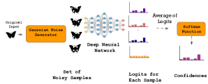
Figure 1. Schematic of LDL. LDL constructs a high dimensional sphere of label invariance around each sample in a manner such that decisions of the model remain unchanged for noisy variants of the sample contained in the sphere. LDL computes the average of confidence scores obtained for each sample in the ensemble and returns the label with highest confidence value.

The demonstrated success of LAB MIAs (Abadi et al., 2016; Carlini et al., 2019; Jia et al., 2019) necessitates developing techniques to mitigate their impact. Since retraining DNNs is often impractical in many applications, as noted in (Carlini and Wagner, 2017), a question is whether one can develop methods to mitigate the impact of LAB MIAs on DNN models that have already been deployed. We provide an affirmative answer to this question by proposing LDL, a Light weight Defense against LAB MIAs that can be incorporated into already-deployed DNN models without needing to retrain them. Fig. 1 presents a schematic of LDL.

Our Contribution: Our focus is on DNN models that perform a classification task whose objective is to identify the most relevant class out of a set of possible choices for each sample. We assume that an adversary can carry out a LAB MIA (Choquette-Choo et al., 2021; Li and Zhang, 2021) to identify samples that were used to train the model. We develop LDL, a defense against LAB MIAs, that does not require retraining of DNNs. LDL employs a randomization technique such that all data points within a high-dimensional sphere of a chosen radius parameter with the input sample at the center of the sphere return the same label. This type of label smoothing over the high-dimensional sphere aims to prevent an adversary carrying out a LAB MIA from identifying whether the sample is a member or not. Specifically, our contributions are:

• We provide an analytical characterization of the effectiveness of an adversary carrying out a LAB MIA when LDL is deployed, and examine how it varies with the magnitude of noise that will be required to misclassify samples.

• We estimate the magnitude of perturbation required to misclassify samples using adversarial noise learning methods (Goodfellow et al., 2015). We observe that deploying LDL ensures that misclassification rates accomplished by the addition of adversarial noise is similar for both members (training dataset) and nonmembers (testing dataset), making it difficult for an adversary to successfully carry out a LAB MIA.

• We evaluate LDL against state-of-the-art (SOTA) LAB MIAs (Choquette-Choo et al., 2021; Li and Zhang, 2021) on four image datasets– CIFAR-10, CIFAR-100, GTSRB, Face– and three non-image datasets– Purchase, Texas, and Location. We consider two distinct adversary types: (i) a weak adversary that only has knowledge of feature values of samples in its possession, and (ii) a strong adversary that has knowledge of both, sample features and their corresponding labels. In each case, we observe that using LDL results in a significant reduction in the attack success rate of LAB MIAs.

• We empirically demonstrate that despite not needing to retrain the DNN, using LDL achieves classification accuracy and adversary success rates that are comparable to other defenses against LAB MIAs (Abadi et al., 2016; Nasr et al., 2018; Srivastava et al., 2014) which require that the DNN model be retrained.

The rest of the paper is organized as follows: Section 2 provides background on DNNs, MIAs, and metrics to evaluate the attack performance. Section 3 describes the adversary model and gives an overview of our defense strategy. Section 4 introduces LDL, a defense against LAB MIAs that obviates a need to retrain models. Sections 5 and 6 discuss evaluation of LDL and reports our experimental results. Section 7 discusses extensions of LDL to other domains and possible future directions of research. Section 8 summarizes related work and Section 9 concludes the paper.

2. Background

In this section, we provide the necessary background on DNNs, MIAs, and metrics used to evaluate attack performance.

Deep Neural Network (DNN) Classifiers: DNN classifiers take an input $x_{i}$, and return a weight for each class ($Z_{i}=[z_{i1},z_{i2},\cdots,z_{ic}]$ called logits, where $c$ is the number of classes). The softmax function is used to translate these weights to probabilities, where:

(1) $$\texttt{softmax}(Z_{i})=\frac{1}{\sum_{k}e^{z_{ik}}}[e^{z_{i1}},e^{z_{i2}},\cdots,e^{z_{ic}}].$$

The probability/confidence that a sample $x_{i}$ belongs to class $j$ is $p_{ij}=\frac{e^{z_{ij}}}{\sum_{k}e^{z_{ik}}}$. We call the class with highest confidence the decision of DNN classifier. Let $Y^{*}_{i}$ be the true label of $x_{i}$ i.e., $Y_{i}^{*}=[y_{i1},y_{i2},\cdots,y_{ic}]$ and $y_{ij}=1$ if $x_{i}$ belongs to class $j$, otherwise $y_{ij}=0$. DNN classifiers return a non-zero probability for each class . An input is assigned to the class with highest confidence value i.e., $x_{i}$ is assigned to class $k$ if and only if $p_{ik}>p_{ij}\forall j\in\{1,\cdots,k-1,k+1,\cdots,c\}$. Loss functions quantify the difference between the ideal output ($Y_{i}^{*}$) and the observed output ($P_{i}=[p_{i1},\cdots,p_{ic}]$). The cross entropy loss is widely used in ML and is defined as:

(2) $$\mathit{l_{CE}}(P_{i},Y_{i}^{*})=-\sum_{j=1}^{c}y_{ij}\log p_{ij}.$$

A DNN classifier is called overfitted if the model classifies members (samples in the training set) correctly with high confidence while having lower accuracy when identifying nonmembers (Shokri et al., 2017). Consequently, loss values for members would be low, while those for nonmembers will be high. In (Jia et al., 2019), it was shown that overfitting of DNNs during training makes the model vulnerable to MIAs.

Membership Inference Attacks (MIAs): MIAs determine whether a sample ($x$) was a member of the training set used to learn a DNN model ($\mathcal{M}$). The effectiveness of an adversary depends on the knowledge ($\mathcal{\phi}$) about the model e.g., the hyper-parameters (Carlini et al., 2019). The adversary uses a function $\mathcal{A}$ that maps an input sample $x$ to $\{0,1\}$, i.e., the function returns $s=1$ if it decides that a given sample $x$ belonged to the training set (member), and $s=0$ otherwise.

Metrics: We assume that samples belonging (not belonging) to the member set, denoted $S_{m}$ ($S_{m}^{\prime}$), have membership label $s=1$ ($s=0$). MIAs aim to predict the membership label ($s_{i}$) of a sample ($x_{i}$).

True Positive Rate (TPR) and True Negative Rate (TNR) indicate correct classification rates for member and nonmember samples, and are defined as ${TPR}=\Pr\{s=1;x\in S_{m}\}$ and ${TNR}=\Pr\{s=0;x\in S_{m}^{\prime}\}$ respectively.

False Positive Rate (FPR) and False Negative Rate (FNR) indicate incorrect classification rates for nonmember and member samples, and are defined as ${FPR}=\Pr\{s=1;x\in S_{m}^{\prime}\}$ and ${FNR}=\Pr\{s=0;x\in S_{m}\}$ respectively.

Attack Success Rate (ASR) measures the average accuracy of the MIA in distinguishing members from nonmembers, which is defined as:

(3) $${ASR}=\frac{TPR+TNR}{2}.$$

3. System Model

In this section we describe overfitted DNN models and label-based MIAs (LAB MIAs), then present the adversary model and provide an overview of our defense methodology.

3.1. Overfitted DNN Models

Overfitting in DNN models can occur when member (training or seen) samples are learned extremely well by ‘memorizing’ patterns in the data and noise fluctuations (Hastie et al., 2009). As a consequence, the model will be unable to classify nonmember (test or unseen) samples effectively. Overfitting is a major reason for the feasibility of MIAs. It has been shown in (Yeom et al., 2018) that an adversary will be able to use loss or confidence values to effectively distinguish between member and nonmember samples of an overfitted model.

One method to quantify the information obtained by an adversary carrying out a MIA on overfitted DNN models is to evaluate a gap attack, as defined in (Yeom et al., 2018; Choquette-Choo et al., 2021). The gap attack is a MIA that infers membership using the fact that for an overfitted model, a sample belonging to the training dataset is classified correctly with high confidence, whereas a nonmember sample is likely to be misclassified with high confidence (Choquette-Choo et al., 2021). The $ASR$ of an adversary carrying out a gap attack is denoted $ASR_{gap}$. We note that $TPR$ in Eqn. (3) is the accuracy of classification of member data samples, and denoted as $Acc_{mem}$. For nonmmembe samples, classification accuracy of the DNN is denoted as $Acc_{nonmem}$. When a nonmember sample provided as input to the DNN by the adversary is correctly classified, the adversary is led to conclude, albeit incorrectly, that this sample belongs to the member set. Hence, the $TNR$ in Eqn. (3) is given by $1-Acc_{nonmem}$. Substituting these values in Eqn. (3) yields the expression given in (Yeom et al., 2018; Choquette-Choo et al., 2021):

(4) $${ASR}_{gap}=0.5+\frac{Acc_{mem}-Acc_{nonmem}}{2}=0.5+\frac{TPR-FPR}{2}$$

It has been noted in (Choquette-Choo et al., 2021) that the gap attack overestimates the value of $Acc_{nonmem}$ (since any misclassified sample is identified as a nonmember). Carrying out a more deliberate MIA, such as a LAB MIA, will typically enable an adversary to achieve $ASR\geq ASR_{gap}$ through additional queries to the DNN model to obtain a better estimate of $Acc_{nonmem}$. The objective of any defense against MIAs is to reduce the value of $ASR$ to the minimum possible, i.e., $\max\{ASR_{gap},0.5\}$. In this paper, we examine the impact of deploying LDL on the ASR of an adversary carrying out a LAB MIA on an overfitted DNN model with varying sizes of training datasets.

3.2. Label-Based MIAs (LAB MIAs) on DNNs

Given the final label of a sample output by a DNN model, an adversary carrying out a LAB MIA (Choquette-Choo et al., 2021; Li and Zhang, 2021) uses adversarial learning methods (Chen et al., 2020) to estimate the amount of adversarial noise needed to be added to the sample to make the DNN misclassify the sample. The magnitude of noise will enable distinguishing members from nonmembers, as explained next.

An overfitted DNN model will classify member samples with high confidence, since these samples are far away from a decision boundary. For example, for a classifier that uses a binary logistic regression model $\rho(x):=\frac{1}{1+e^{-(\omega^{T}x+b)}}$, the distance of a sample $x$ to the decision boundary is $(\omega^{T}x+b)/\|\omega\|_{2}$. Then, samples with higher confidence will have a larger distance to the decision boundary (since $(\omega^{T}x+b)\rightarrow\infty\Rightarrow\rho(x)\rightarrow 1$). As shown in (Choquette-Choo et al., 2021), computing this distance will be equivalent to determining the smallest magnitude of additive noise required to make the DNN misclassify the sample. Member samples will require a larger magnitude of noise for misclassification compared to nonmember samples. It was noted in (Choquette-Choo et al., 2021; Li and Zhang, 2021) that LAB MIAs only required the final sample label, and did not require knowledge of confidence values associated to labels.

3.3. Adversary Model for LAB MIAs

We follow the setting considered in (Choquette-Choo et al., 2021; Li and Zhang, 2021), and assume that the adversary has black-box model access, and that the DNN model only returns a label for a given input. Thus, model hyper-parameters are not not known to the adversary, but the adversary can obtain the output for any sample provided to the model. The adversary aims to determine whether a sample belongs to the training set of a DNN model ($s_{i}=1$ if $x_{i}\in S_{m}$, otherwise $s_{i}=0$) by analyzing outputs of the model. Similar to (Li and Zhang, 2021), we consider two types of adversaries: (i) an adversary with access to a small subset of member and nonmember samples. These samples can be used to assess the behavior of the DNN model by examining the magnitude of noise that needs to be added in order for the model to misclassify them; and (ii) an adversary that does not have any knowledge about samples used to train the DNN model. In this case, as noted in (Li and Zhang, 2021), the LAB MIA adversary uses substitute models to estimate the magnitude of noise required to misclassify members and nonmembers of the substitute model.

Weak vs. Strong adversary: Any adversary carrying out a LAB MIA will have full knowledge of features of samples that are in its possession. The adversary examines the output of the DNN model for a sample that it perturbed with additive noise. A strong adversary has knowledge of sample features and the corresponding label of the sample. A weak adversary only has knowledge of features of samples in its possession. The weak adversary will be able to obtain the label associated to the sample by examining the output of the DNN when the sample is given as input. The procedure to carry out a LAB MIA will then be identical for both types of adversaries.

3.4. Defense Strategy Against LAB MIAs

We assume that the owner of the DNN model uses a defense mechanism to mitigate information leakage about samples used to train this model. The objective of the defense strategy is to ensure that the amount of perturbation required to misclassify members and nonmembers will be of a comparable magnitude. As noted in (Choquette-Choo et al., 2021; Li and Zhang, 2021), the owner of the DNN model does not have any additional computational resources beyond those used for model inference, and will not be able to retrain the DNN model.

In this paper we propose LDL, a light weight defense against LAB MIAs. LDL works by constructing a high-dimensional sphere around queried samples such that the model decision is unchanged for (noisy) variants of the sample within the sphere. Using LDL as a defense does not require retraining the DNN model or additional computational resources beyond those needed for inference. We describe LDL in detail in Section 4.

4. Our Proposed Defense

In this section, we first describe the insight behind our method and then describe the implementation of LDL in detail.

4.1. Description of LDL

The objective of LDL is to ensure that magnitudes of noise required for misclassification of members and nonmembers are comparable. This will ensure indistinguishability of members and nonmembers to an adversary carrying out a LAB MIA. LDL uses randomization at inference time and constructs a label invariant sphere around samples. Following (Cohen et al., 2019), we term a classifier $f$ with randomization as a smoothed classifier $g$. The smoothed classifier $g$ returns the class that $f$ will most likely return for perturbed variants of $x$ (as opposed to the original sample $x$). Although the smoothed classifier $g$ may not return the true label of $x$, it is guaranteed to return the same label for all $x^{\prime}$ inside a sphere of radius $r$ centered at $x$ (Cohen et al., 2019). LDL achieves a reduction in the attack success rate of LAB MIAs that use additive noise to infer whether a sample belongs to the training set (member) or not (nonmember).

We note that the term $ASR_{gap}$ in Eqn. (4) is specifically defined for the gap attack (Choquette-Choo et al., 2021), and will not be adequate to quantify the success rates of other classes of MIAs. Moreover, Eqn. (4) does not capture the effectiveness of defense mechanisms that might be used by a DNN model to mitigate the impact of a MIA. Therefore, the quantification of ASR when using a defense mechanism such as LDL should capture the following properties: (i) when LDL is not deployed by the DNN model, it should precisely model the attack success rate, (ii) when LDL is deployed, it should express the ASR as a function of randomization parameters, (iii) as the amount of randomization used by LDL increases, the attack success rate should approach $50\%$, since its strategy will then reduce to a fair coin-toss, and (iv) when LDL is not deployed as a defense and the adversary carries out a gap attack, we should recover Eqn. (4) that was presented in (Choquette-Choo et al., 2021). Following the above criteria, we propose that the attack success rate (in Eqn. (4)) when LDL is deployed takes the modified form:

(5) $$ASR_{LDL}=0.5+(1-h(\sigma^{2}))\frac{{TPR}-{FPR}}{2},$$

where ${TPR}$ and ${FPR}$ are the adversary’s true positive rate and false positive rates as defined in Sec. 2. Here, $h(\sigma^{2})\in[0,1]$ is a function that has the following properties: (a) $h(\sigma^{2})=0$ if $\sigma=0$, (b) $h(\sigma^{2})$ is monotone increasing with respect to $\sigma$, (c) $h(\sigma^{2})=1$ as $\sigma\rightarrow\infty$, and (d) if $h(\sigma^{2})=0$ and ${TPR}-{FPR}=Acc_{mem}-Acc_{nonmem}$, $ASR_{LDL}$ reduces to $ASR_{gap}$. These properties model all the criteria (i) - (iv) identified above.

Moreover, when LDL is deployed with $\sigma^{2}>0$, we observe that $ASR_{LDL}<ASR_{gap}$, since: (i) as $\sigma^{2}$ increases, the TPR of the adversary decreases while the FPR increases, and (ii) $h(\sigma^{2})\geq 0$ for $\sigma^{2}>0$. This formulation is adequate to quantify the ASR of a wide range of MIAs, depending on the function $h(\sigma^{2})$. Two pertinent choices that we will use in our experimentas in Sec. 6 are $h_{1}(\sigma^{2}):=1-\exp{(-\alpha\sigma^{2})}$, and $h_{2}(\sigma^{2}):=L(1+\exp{(-\beta(\sigma^{2}-c)))^{-1}}$, where $\alpha,\beta,L,c>0$.

4.2. Implementation of LDL

As noted in (Choquette-Choo et al., 2021; Li and Zhang, 2021) and from the example in Sec. 3.2, samples with lower confidence will be located closer to a decision boundary of a DNN model. An adversary carrying out a LAB MIA can either use learning methods that require only black-box access to the model (Chen et al., 2020) or add an arbitrary amount of noise (random) to the input data sample to estimate the distance to the decision boundary. In each case, LDL constructs a sphere centered at a sample in a manner that the model returns the same label for all perturbed variants of the sample contained in the sphere. This aims to create an ambiguity for the adversary who tries to distinguish between members and nonmembers. To construct the label-invariant sphere around samples, LDL uses a smoothed classifier $g$ that aims to return the same label for variants of $x$ that satisfy ($x+\delta,\>\>\|\delta\|_{2}\leq r$). We assume that a zero-mean Gaussian noise with variance $\sigma^{2}$ is used to perturb $x$. Algorithm 1 illustrates the working of LDL. For each input $x$, we obtain $K$ perturbed variants of $x$ and determine the logit of the model for each perturbed sample. We then calculate the average of the logits (ensemble of decisions). We compute confidence scores for each class through a softmax function. Using a smoothed classifier increases the amount of noise required to change a decision of the original model for members and nonmembers. As a result, an adversary will not be able to accurately estimate the magnitude of the perturbation required for misclassification.

Algorithm 1 LDL: Light weight Defense against LAB MIAs

1:$x,f,{\sigma}^{2}$;

2:for all $i=1:T$ do

3:     $n_{i}\sim\mathcal{N}(0,\sigma^{2}I);\>\>\>x_{noisy}\leftarrow x+n_{i}$;

4:     predictions $\leftarrow$ predictions $\cup f(x_{noisy})$;

5:end for

6:prediction $\leftarrow$ average(predictions);

7:return prediction;

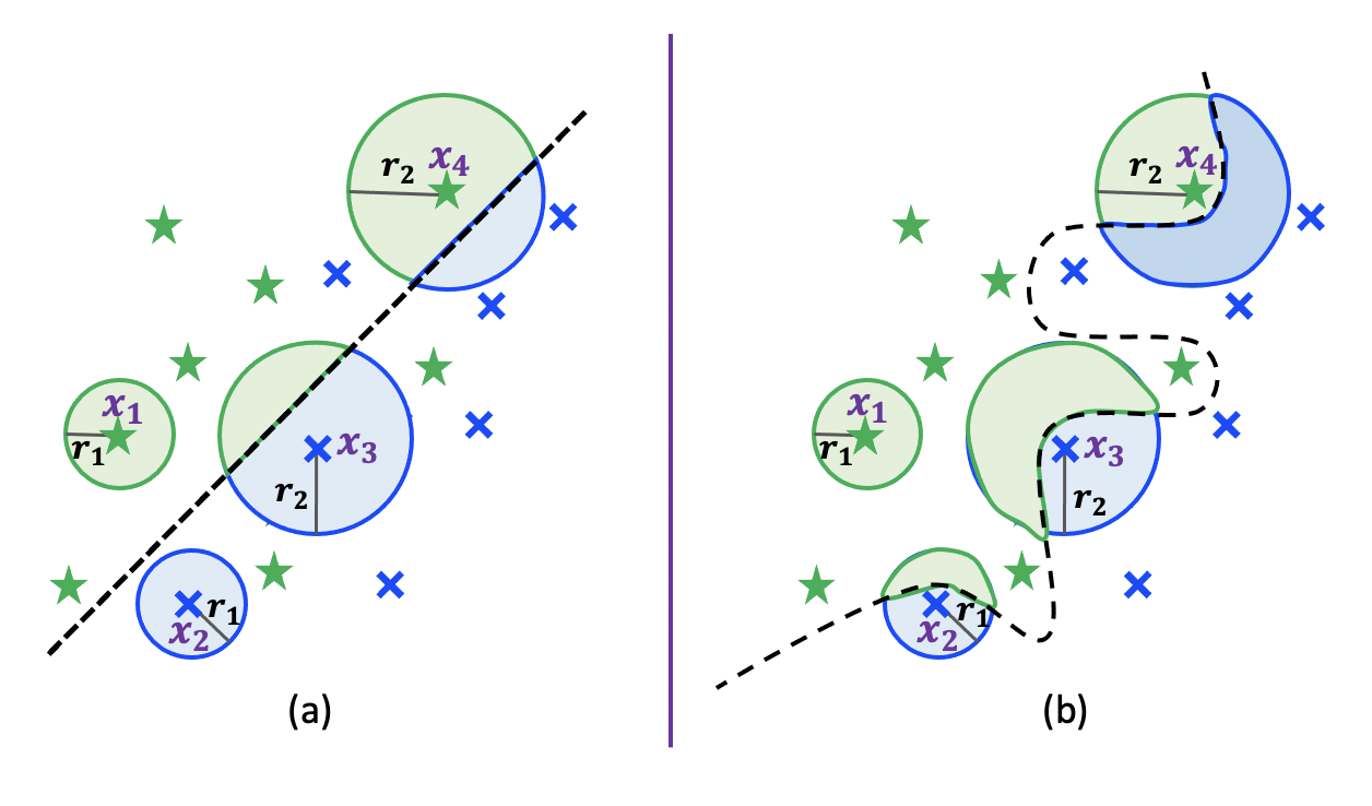
Figure 2. Representation of high-dimensional spheres of label invariance of different radii on normal and overfitted models. The figure shows two classes (green and blue) separated by a decision boundary (dashed black line). In Fig. 2(a), we see that spheres of radius $r_{1}$ or $r_{2}$ ($>r_{1}$) result in correct classification of samples (e.g., $x_{3}$ is classified to the blue class since area of the blue region within the sphere centered at $x_{3}$ is larger than that of the green region.). Thus, an adversary will require a perturbation $>r_{2}$ for the model to misclassify samples. The shape of the decision boundary in Fig. 2(b) indicates an overfitted model. In this case, even a smaller value of $r$ (i.e., $r_{1}$) can result in samples being misclassified.

Figure 2(a) illustrates that a larger radius increases robustness of samples to noise. For example, samples in the sphere of radius $r_{2}$ around $x_{3}$ mostly belong to the blue class. LDL thus classifies $x_{3}$ and any perturbed variant of $x_{3}$ within this sphere to the blue class. As a result, an adversary will require a perturbation larger than $r_{2}$ for the model to misclassify $x_{3}$. However, when an adequate decision boundary is not learned, such as for overfitted DNNs, even a small amount of perturbation ($r_{1}<r_{2}$) can result in misclassification of samples by the DNN. This is illustrated in Fig. 2(b), where samples $x_{3}$ and $x_{4}$, which would otherwise be correctly classified by the model, will be misclassified after deploying LDL with radius $r_{2}$. The radius of the label-invariant sphere is related to the value of the parameter $\sigma^{2}$. This has the following consequence. From Sec. 4.1 and Eqn. (5), an increase in $\sigma^{2}$, and correspondingly, the radius of the sphere, will cause a reduction in the value of $ASR_{LDL}$.

5. Evaluation of LDL Performance

In this section, we describe the settings under which we evaluate LDL, and describe the datasets that we use.

5.1. Evaluation Setup

We experimentally evaluate the performance of LDL against SOTA LAB MIAs (Choquette-Choo et al., 2021; Li and Zhang, 2021). In each case, for any input, the DNN model only returns the label with the highest confidence. LAB MIAs estimate the amount of noise required to make the DNN model change its decision in order to distinguish between members and nonmembers. When the DNN model does not incorporate/deploy any defense against a LAB MIA, we call it a defense-free model. We compare the success rate of an adversary ($ASR$) carrying out a LAB MIA on a defense-free model and in the case when LDL is used as a defense.

We evaluate LDL against a weak and a strong adversary defined in Sec. 3.3. As noted in Sec. 3.3, a strong adversary has knowledge of true labels. For a strong adversary, we hypothesize that the value of $ASR$ when LDL is deployed will be close to $ASR_{gap}$, since it has knowledge of values of $TPR$ and $FPR$ (Eqn. (5). Similarly, from Sec. 3.3, a weak adversary has knowledge of only feature values of samples. For a weak adversary, we hypothesize that using LDL will reduce the $ASR$ of a LAB MIA to $50\%$, since a sample will be identified as a member or a nonmember from the outcome of a fair coin toss. As described in Sec. 3.3, we consider two settings: (i) when the adversary has a small set of member and nonmember samples (Li and Zhang, 2021), it learns the optimum value of a threshold that separates members from nonmembers. (ii) when the adversary has no knowledge about which samples may have been used to train the DNN model, it locally learns a substitute model (Choquette-Choo et al., 2021) to estimate the minimum amount of noise required to misclassify samples. The amount of noise required to be added to a sample to trigger misclassification can be estimated using adversarial learning methods (adversarial noise) as shown in  (Chen et al., 2020), or by generating perturbed variants of each sample (random noise), as in (Choquette-Choo et al., 2021).

Adversarial Noise: Since the adversary has only black-box access to the DNN model, it uses query-based methods to learn the minimum amount of noise required to cause the DNN model to misclassify the sample. In generating adversarial noise, to maintain consistency with (Choquette-Choo et al., 2021; Li and Zhang, 2021), we use a query-based adversarial learning method called HopSkipJump (Chen et al., 2020) to estimate the minimum magnitude of noise perturbation that has to be added to the input sample point for misclassification.

Random Noise: In this case, the LAB MIA adversary uses a random additive noise to estimate the distance of a sample to the decision boundary (Choquette-Choo et al., 2021). Varying amounts of noise are used to generate multiple perturbed samples and the adversary learns the smallest amount of noise required to trigger a misclassification by the DNN model.

5.2. Datasets and Classifiers

We use all the datasets noted in (Li and Zhang, 2021), including (i) CIFAR-10 (Krizhevsky and Hinton, 2009), (ii) CIFAR-100 (Krizhevsky and Hinton, 2009), (iii) GTSRB (Houben et al., 2013), and (iv) Face (Huang et al., 2012) for our experiments. We remove classes with $<40$ images from the Face dataset. To train DNN models for classification tasks, we construct a convolutional neural network with 4 convolutional layers and 4 pooling layers with 2 hidden layers, each containing at least 256 units. We train them for 200 epochs using the Adam optimizer.

We also evaluate LDL on three non-image datasets, as noted in (Shokri et al., 2017), which includes (i) Location, (ii) Purchase, and (iii) Texas. Unlike image datasets that have continuous feature values, features of these three datasets take discrete values. We use the same settings as in (Choquette-Choo et al., 2021), and train a fully connected neural network with one hidden layer of size of 128 for the Purchase dataset, a fully connected neural network with two hidden layers of size 128 and a Tanh activation function for the Location and Texas datasets. Our code is available on our Github page at https://tinyurl.com/mpzb3j5y.

6. Results of Experiments

This section presents results of our experimental evaluations. We use the same datasets and experiment settings from SOTA LAB MIAs (Choquette-Choo et al., 2021; Li and Zhang, 2021), and also compare LDL to other defenses against MIAs. In Sec. 6.1 and 6.2, we evaluate the performance of LDL against an adversary carrying out a LAB MIA using adversarial noise and random noise (described in Sec. 5.1). In Sec. 6.3, we examine the effect of deploying LDL against an adversary that uses substitute models when it does not have access to the set of member and nonmember samples. Section 6.4 shows that deploying LDL ensures that misclassification rates accomplished by the addition of adversarial noise is similar for both members and nonmembers, making it difficult for an adversary to successfully carry out a LAB MIA. In Sec. 6.5, we demonstrate that despite not needing to retrain DNN models, LDL performs favorably in comparison to other defenses againt LAB MIAs that require DNN models to be retrained. We examine the consistency of observed values of $ASR_{LDL}$ with the analytical characterization from Eqn. (5) in Sec. 6.6.

	Strong Adversary	Weak Adversary
CIFAR-10
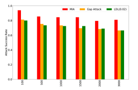
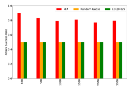
CIFAR-100

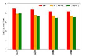
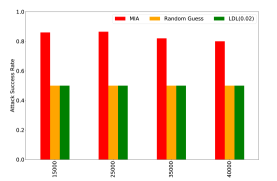
Figure 3. Attack success rate (ASR) of adversary carrying out a LAB MIA using HopSkipJump adversarial noise (Li and Zhang, 2021) for defense-free models (red bars) and models with LDL deployed (green bars). We evaluate LDL on datasets with different sizes of training sets for a strong adversary (left column) and a weak adversary (right column). We show results for the CIFAR-10 and CIFAR-100 datasets here; results for the GTSRB and Face datasets are presented in the Appendix. The value of $ASR_{gap}$ for a strong adversary carrying out a gap attack and that of a random guess for a weak adversary on a defense-free model are also shown (orange bars). Deploying LDL successfully reduces the $ASR$ to a value close to $ASR_{gap}$ for a strong adversary and to $50\%$ for a weak adversary.

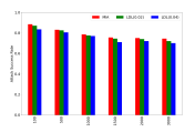
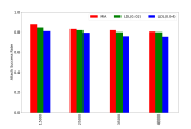
(a) CIFAR-10	(b) CIFAR-100
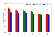
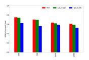
(c) GTSRB	(d) Face

Figure 4. Success rate of a LAB MIA that uses random noise to estimate the distance of a sample to a decision boundary. Values of the attack success rate ($ASR$) for a defense-free model (red bars) and model with LDL deployed using different values of $\sigma^{2}$ (green and blue bars) are shown. Consistent with Eqn. (5), a larger value of $\sigma^{2}$ provides a greater reduction the value of $ASR$.

Defense-free
LDL(0.02)
	(a) CIFAR-10	(b) CIFAR-100	(c) GTSRB	(d) Face

Figure 5. t-SNE representation of separability of members and nonmembers for 4 datasets. We calculate ${score_{G}}(x)$ for 10 different values of $\sigma^{\prime}$ and use t-SNE to translate them to a $2D-$representation. For defense-free models (top row), there is a region denoted by the dashed ellipse that enables an adversary to easily identify nonmembers. In comparison, LDL successfully prevents an adversary from distinguishing members from nonmembers since there is no region that clearly separates these two (blue and red dots on graphs in bottom row).

6.1. LDL vs. Adversary using Adversarial Noise

We evaluate LDL against an adversary carrying out a LAB MIA. The adversary uses a black-box adversarial model HopSkipJump (Chen et al., 2020) to estimate the minimum adversarial noise required to cause the DNN model to misclassify a sample. To distinguish members from nonmembers, the adversary estimates the best threshold on the minimum amount of noise needed to separate them  (Li and Zhang, 2021). Our objective is to demonstrate that using LDL effectively reduces the $ASR$ value, i.e., the ability of the adversary to distinguish members from nonmembers. We examine whether LDL successfully reduces the value of $ASR$ to $ASR_{gap}$ for a strong adversary (Eqn. (4) and (5)). For a weak adversary, we examine if LDL successfully reduces the value of $ASR$ to $0.5$, which corresponds to tossing a fair coin.

Fig. 3 shows the $ASR$ for defense-free models (MIA, red bars) and models with LDL (green bars). Our experiments reveal that deploying LDL hinders an adversary using HopSkipJump to determine the minimum magnitude of noise required to misclassify samples.

Strong adversary: A strong adversary can carry out a gap attack (Choquette-Choo et al., 2021) (Sec 3.1), which identifies a sample as a member if it is classified correctly by the DNN model, and a nonmember otherwise. The success rate of the adversary carrying out a gap attack is given by $ASR_{gap}$ in Eqn. (4). Similar to (Choquette-Choo et al., 2021), we use the value of $ASR_{gap}$ as a benchmark to evaluate how well LDL reduces the $ASR$ of LAB MIAs. Reducing the $ASR$ below $ASR_{gap}$ by a large amount will affect classification accuracy of the model ($Acc_{mem},Acc_{nonmem}$ terms in Eqn. (4)). The left column of Fig. 3 demonstrates that while the adversary has a high $ASR$ value when carrying out a LAB MIA on defense-free DNN models (red bars), using LDL reduces the $ASR$ to near $ASR_{gap}$ (green and orange bars are comparable).

Weak adversary: A weak adversary assumes that the decision of the DNN model is the true label (Sec 3.3). In this case, we use $50\%$ (i.e., a fair coin-toss) as a benchmark (orange bars in Fig. 3 right column) to evaluate the performance of LDL. The right column of Fig. 3 indicates that in the defense-free case, a weak adversary carrying out a LAB MIA can achieve high $ASR$ even when using the output of the DNN model as the true label (red bars). Using LDL reduces $ASR$ to $50\%$ for the weak adversary (orange and green bars are comparable), thus making members and nonmembers indistinguishable.

6.2. LDL vs. Adversary using Random Noise

Instead of using adversarial noise to estimate the magnitude of noise for misclassification, the adversary can also use random noise to estimate distance to the decision boundary. Such an approach was shown to be successful in (Choquette-Choo et al., 2021). We use a Gaussian noise, $n\sim\mathcal{N}(0,{\sigma^{\prime}}^{2}I)$ and generate $K$ perturbed variants for each sample $x$. The adversary chooses the value of $K$ as the lower bound on the number of perturbed samples beyond which the ASR would not increase. This is indeed an empirical parameter, and for datasets that we use from SOTA LAB MIAs (Choquette-Choo et al., 2021; Li and Zhang, 2021), we empirically found this value to be around $K=1000$. The fraction of samples that are classified correctly is computed as:

(6) $$\texttt{score}_{G}(x,{\sigma^{\prime}}^{2}):=\frac{1}{K}\sum_{i}^{K}\mathbb{I}(g(x+n_{i})==y),$$

where $\mathbb{I}(t)$ returns $1$ if $t$ is true and $0$ otherwise, $g(\cdot)$ returns the predicted label for the perturbed variant of input $x$, and $y$ is the true label of $x$. We observe that for smaller values of ${\sigma^{\prime}}^{2}$, $\texttt{score}_{G}(x,{\sigma^{\prime}}^{2})$ is lower for members than for nonmembers. A justification for this observation is that members are less likely to be misclassified for small perturbations since they are typically located far from a decision boundary (Shokri et al., 2017; Li and Zhang, 2021; Choquette-Choo et al., 2021).

Fig. 4 shows the $ASR$ of an adversary that uses random noise to carry out a LAB MIA. We observe that the $ASR$ value for the defense-free setting is lower for an adversary carrying out a LAB MIA using random noise than when using adversarial noise (red bars in Fig. 4 are lower than red bars of Fig. 3). A reason for this is that adversarial learning techniques aim to optimize the minimum noise required for misclassification. In comparison, random noise is a heuristic used by the adversary. To reduce the value of $ASR$, we will require a larger value of $\sigma^{2}$ as shown by the blue bars of Fig. 4. A larger $\sigma^{2}$ corresponds to a label-invariant sphere of larger radius. Consequently, the adversary would require to add a noise of larger magnitude in order for samples to be misclassified. These observations are consistent with the insight underpinning LDL described in Sec. 4.1 and Eqn. (5).

In Eqn. (6), we had computed $\texttt{score}_{G}(x,{\sigma^{\prime}}^{2})$ for each sample $x$. We collect values of $\texttt{score}_{G}(x,{\sigma^{\prime}}^{2})$ for $10$ different ${\sigma^{\prime}}^{2}$ into a vector, denoted by $\texttt{score}_{G}(x)$. We use a t-distributed stochastic neighbor embedding (t-SNE) (Van der Maaten and Hinton, 2008) to demonstrate that deploying LDL reduces the ability of an adversary to distinguish members from nonmembers. The t-SNE is a technique to visualize high-dimensional data through a two or three dimensional representation.

Fig. 5 shows that score vectors for members and nonmembers before LDL is deployed can be easily distinguished from each other, since there is a region that completely consists of only nonmembers (dashed ellipse in top row). However, after deploying LDL, it becomes difficult for the adversary to distinguish members from nonmembers (bottom row).

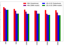
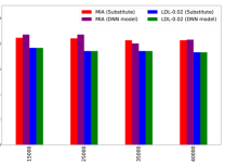
(a) CIFAR-10	(b) CIFAR-100
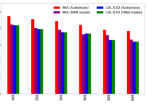
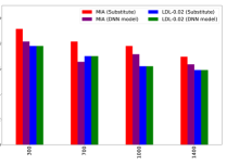
(c) GTSRB	(d) Face

Figure 6. The success rate of LAB MIAs using HopSkipJump for adversary with a substitute classifier (Li and Zhang, 2021). The adversary uses a local substitute classifier to estimate a threshold for distinguishing the minimum required perturbation for misclassification of members and nonmembers. The smallest amount of adversarial noise required to misclassify each sample by the DNN classifier is estimated using HopSkipJump. The threshold is then used to identify a sample as a member or nonmember. Red bars show attack success rate (ASR) of an adversary carrying out a LAB MIA on a defense-free substitute classifier and purple bars show ASR on a defense-free variant of the DNN classifier using the threshold. Blue and green bars show the ASR of substitute and DNN classifiers after deploying LDL. We observe that deploying LDL reduces the ASR of LAB MIAs. Further, the substitute models learned by the adversary are a good representation of the DNN model (blue and green bars are almost equal).

6.3. LDL vs. Adversary using Substitute Models

An adversary may not have access to member and nonmember samples to allow it to estimate the minimum amount of noise required to be added in order to misclassify the sample. However, it might have access to a dataset of other samples along with their labels. In such a scenario, the authors of (Choquette-Choo et al., 2021) suggested using a substitute model (also termed shadow model (Choquette-Choo et al., 2021)) trained locally by a strong adversary. They assumed that the adversary knew the structure of the DNN model and used this to train a substitute model with the same structure on their own dataset. This enabled the adversary to estimate the distance of members and nonmembers to a classification decision boundary. Using this information, the minimum adversarial noise required to misclassify each sample in the DNN model was computed using HopSkipJump (Chen et al., 2020). The adversary then applied a locally estimated threshold (from the substitute model) to distinguish members from nonmembers. Fig. 6 indicates that an adversary using a substitute model to carry out a LAB MIA can effectively distinguish between members and nonmembers (red and purple bars). Deploying LDL with $\sigma^{2}=0.02$ (green and blue bars) successfully reduces the the value of $ASR$. Similar values of $ASR$ observed for substitute (blue bars in Fig. 6) and DNN models (green bars) indicate that the substitute models learned by the adversary are a good representation of the DNN model. The results in this case are also consistent with our observation in Fig. 3 where LDL was able to reduce the value of $ASR$ against a strong adversary employing HopSkipJump to carry out a LAB MIA.

Nonmembers
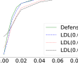
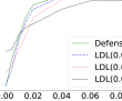
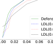
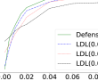
Members
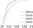
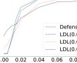
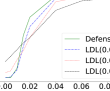
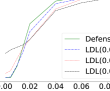
	(a) CIFAR-10 (3000)	(b) CIFAR-10 (2000)	(c) CIFAR-10 (1500)	(d) CIFAR-10 (1000)

Figure 7. Misclassification rates of samples of CIFAR-10 with different sizes of training sets with increasing amounts of noise perturbation $\epsilon$. Deploying LDL ensures that the misclassification rate accomplished by the addition of adversarial noise is similar for both members (training dataset) and nonmembers (testing dataset) in each case.

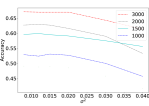
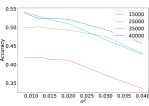
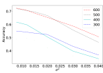
(a) CIFAR-10	(b) CIFAR-100	(c) GTSRB	(d) Face

Figure 8. Classification accuracy on nonmember samples vs. magnitude of perturbation $\sigma^{2}$ when LDL is deployed on 4 datasets- CIFAR10, CIFAR100, GTSRB, Face- with different sizes of training data. The classification accuracy reduces with increasing $\sigma^{2}$.

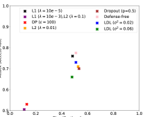
Figure 9. Classification accuracy and $ASR$ for defenses used against a LAB MIA on CIFAR-10 with training set size of $2000$. We observe that LDL with a small value of $\sigma=0.02$ results in a lower $ASR$ while maintaining classification accuracy compared to defenses that aim to reduce model overfitting at the training stage. Using LDL with a larger value of $\sigma=0.06$ reduces the $ASR$, but also lowers classification accuracy. LDL achieves these values without retraining the DNN model.

Non-Image Datasets: We evaluate LDL on three non-image datasets (Shokri et al., 2017; Choquette-Choo et al., 2021; Li and Zhang, 2021) (Purchase, Texas, and Location) characterized by binary-valued features. Discrete feature values prevent addition of Gaussian noise to obtain noisy variants of samples as we have done for experiments on image-based datasets in this section. Instead, we use a Bernoulli distribution with parameter $p\in(0,1)$ to generate $10000$ noisy variants of each sample. The choice of the value of $p$ is informed by the number of features of samples in the dataset. Table 1 indicates that a higher value of the parameter $p$ of the Bernoulli distribution will cause a reduction in classification accuracy and $ASR$. A possible reason for this is that the addition of Bernoulli noise can ‘flip’ the values of features from $0$ to $1$ or vice-versa. This has a more drastic effect on samples when features are discrete compared to the case when they are continuous valued.

Dataset	Defense	Classification Accuracy	ASR
Purchase	Defense-free	$100\%(65.5\%)$	$85.75\%$
	LDL ($p=0.0166$)	$59(13.5\%)$	$69\%$
Location	Defense-free	$100\%(55.0\%)$	$92.5\%$
	LDL ($p=0.0022$)	$100(30\%)$	$91.25\%$
	LDL ($p=0.011$)	$98.5\%(15.5)$	$80.25\%$
Texas	Defense-free	$100\%(54.5\%)$	$83.5\%$
	LDL ($p=0.00016$)	$54.5\%(26.5\%)$	$69.5\%$
	LDL ($p=0.00032$)	$36\%(17\%)$	$62\%$

Table 1. Classification accuracy for members (nonmembers) and $ASR$ when an adversary carries out a LAB MIA on the Purchase, Texas, and Location datasets with binary-valued features. Perturbed variants of each sample is generated by adding a $Bernoulli(p)$ noise, where the values of the parameter $p$ are determined by the number of features corresponding to samples in the respective dataset. We observe that the ASR is largest when no defense is used against the MIA. When LDL is deployed as a defense, larger values of $p$ are more effective in reducing the value of $ASR$. However, this comes at the cost of simultaneously reducing the classification accuracy.

6.4. Evaluation of Robustness of LDL to Noise Perturbations

In mounting LAB MIAs (Choquette-Choo et al., 2021; Li and Zhang, 2021), an adversary uses the insight that nonmember samples require a smaller amount of additive noise in order to trigger a misclassification by the DNN model compared to members. The sphere of label-invariance constructed by LDL ensures that a sample and all its perturbed variants within this sphere will have the same label. In this section, we empirically evaluate the robustness of LDL to different levels of noise perturbations for varying values of radius of label-invariance $\sigma^{2}$.

We use a SOTA adversarial example generation technique called Fast Gradient Sign (FGS) (Goodfellow et al., 2015) to study the perturbation required to misclassify samples after LDL is deployed. FGS is known to typically require only a single step to determine the magnitude of perturbation required for misclassification (Goodfellow et al., 2015). FGS adds noise perturbation to a ‘clean’ sample $x$ which has the true label $y$ so that a classifier will identify that $x$ belongs to a class $y^{\prime}\neq y$. FGS accomplishes this goal by using the sign of the gradient of a loss function $\mathcal{L}((F(x,\theta),y)$ to compute the needed adversarial input $x_{adv}:=x+\epsilon\times sign(\nabla\mathcal{L}(F(x,\theta),y))$, where $\epsilon$ is the magnitude of perturbation noise added to $x$.

Figure 7 presents misclassification rates of samples of CIFAR-10 with different sizes of training sets with increasing amounts of noise perturbation $\epsilon$. We compare the defense-free case and when LDL is deployed using $\sigma^{2}=\{0.02,0.04,0.06\}$. We observe that deploying LDL ensures that the misclassification rate accomplished by the addition of adversarial noise is similar for both members (training dataset) and nonmembers (testing dataset).

The effect of deploying LDL on classification accuracy will depend on the radius of the sphere constructed by LDL (that depends on $\sigma^{2}$) and the original model itself. Figure 8 shows the change in classification accuracy of nonmember samples as $\sigma^{2}$ increases. We observe that, as expected, the classification accuracy decreases with increasing $\sigma^{2}$. The accuracy drop is sharper for models that are known to be more prone to overfitting, such as GTSRB and Face.

6.5. LDL vs. SOTA Defenses against MIAs

Defenses against MIAs can be divided into two broad categories: (i) distorting outputs of models that are already overfitted, and (ii) training models in a manner to prevent overfitting.

In (i), the impact of MIAs is mitigated by distorting outputs of an overfitted DNN model. Recent methods that have successfully used this approach include Memguard (Jia et al., 2019) and confidence masking (Ye et al., 2022a). Although such methods do not require the DNN model to be retrained, it has been demonstrated in (Choquette-Choo et al., 2021; Li and Zhang, 2021) that they are not effective against an adversary employing a LAB MIA.

In (ii), overfitting of the model is reduced at the training stage; however, this could result in a significant reduction in accuracy. Overfitting can be reduced through methods such as dropout (Srivastava et al., 2014), L1- and L2- regularization (Nasr et al., 2018) or differential privacy (DP) techniques (Abadi et al., 2016). We compare the classification accuracy and ASR of LDL with DP-SGD with a privacy budget $\epsilon=100$ (Abadi et al., 2016) , dropout regularization with dropout probability $p=0.8$ (Srivastava et al., 2014), and L1-regularization with weights $\lambda=10^{-5},10^{-3}$ and L2-regularization with weights $\lambda=0.01,0.1$ (Nasr et al., 2018). Fig. 9 shows that LDL is able to reduce the value of $ASR$ while maintaining classification accuracy compared to defense mechanisms that aim to reduce overfitting. LDL achieves these performance levels without retraining the DNN model.

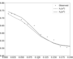
Figure 10. Change in the value of $ASR_{LDL}$ with increasing $\sigma^{2}$ for $h_{1}(\sigma^{2}):=1-\exp{(-4.88\sigma^{2})}$, and $h_{2}(\sigma^{2}):=1.34(1+\exp{(-12.93(\sigma^{2}-0.1))^{-1}}$. The black dots indicate the value of $ASR_{LDL}$ from our experimental evaluations. We observe that both choices of the function $h(\sigma^{2})$ to compute $ASR_{LDL}$ in Eqn. (5) are consistent with the observed values.

6.6. Observed vs. Analytical $ASR_{LDL}$ Values

We examine the correctness of Eqn. (5), which provides an analytical characterization of the success rate of an adversary carrying out a LAB MIA when LDL is deployed as a defense. Fig. 10 illustrates the effect of the choice of the parameter $\sigma^{2}$ on the value of $ASR_{LDL}$ obtained using: (i) our experiments (black dots), (ii) curve fitting to the functions $h_{1}(\sigma^{2}):=1-\exp{(-4.88\sigma^{2})}$ (dashed line) and $h_{2}(\sigma^{2}):=1.34(1+\exp{(-12.93(\sigma^{2}-0.1)))^{-1}}$ (solid line) in Eqn. (5). We observe that results of our experiments agree with both choices of $h(\cdot)$ for values of $\sigma^{2}\in(0,0.2)$.

7. Discussion

Lack of Formal Guarantee: LDL provides a way to protect against LAB MIAs without retraining DNN models, and compares favorably against other defenses that require DNNs to be retrained (Fig. 9). An adversary carrying out a LAB MIA only has black-box (input and output) access to the DNN model. It remains an open problem if additional assumptions on DNN structure can be used to provide a precise characterization on the level of protection offered by LDL against LAB MIAs. A potential approach is to leverage recent results that used polynomial functions to provide bounds on the error in estimating nonlinear activation functions of DNN layers (Hesamifard et al., 2019).

LDL on Discrete Datasets: We evaluate LDL on three datasets–Texas, Purchase, and Location– with discrete-valued features. In these cases, we used a $Ber(p)$ noise to generate perturbed variants of samples (Table 1). Although using LDL was effective in reducing the value of $ASR$ for these datasets, it resulted in a simultaneous reduction in classification accuracy. The lower classification accuracy could occur as a result of the additive noise flipping the label of the sample. In contrast, adding a Gaussian noise to samples in the four datasets with continuous-valued features (CIFAR-10, CIFAR-100, GTSRB, Face) did not change the label of samples as significantly. A possible way to maintain classification accuracy when LDL is used on datasets with discrete-valued features is to investigate the use of a noise generated from a discrete Gaussian distribution (Canonne et al., 2020).

Other Choices of $h(\sigma^{2})$: In this paper, we defined the set of properties that $h(sigma^{2})$ must possess and presented two choices that defined the value of $ASR_{LDL}$ in Eqn. (5), and showed that they were both consistent with our experimental observations (Fig. 10). There can be a class of solutions of $h(\sigma^{2})$ which satisfy the properties identified in Sec. 4.1. Examining and characterizing the effect of the types and sizes of datasets used in experiments on the choice of $h(\sigma^{2})$ remains an open research problem.

8. Related Work

Membership Inference Attacks (MIAs) and Defenses: MIAs aim to determine whether a sample belongs to the training set of a classifier or not. There are three different approaches that an adversary with black-box access to the outputs of its target model can use to distinguish members and non-members. First, the adversary can directly examine the output of the model by studying confidence values or calculating loss values returned by the model (Yeom et al., 2018) . Second, the adversary can learn a model to analyze the difference between outputs of the model for members and nonmembers (Shokri et al., 2017; Ye et al., 2021) . Third, the adversary can examine outputs of the model for perturbed variants of each input sample (Jayaraman et al., 2021). The MIAs of this type presume that models behave differently for perturbed variants of members and nonmembers. However, all the above three types of MIAs are confidence-score based. A new class of label-based MIAs was recently proposed in (Choquette-Choo et al., 2021; Li and Zhang, 2021) where an adversary only required knowledge of labels of samples rather than the associated confidence scores. These works demonstrated that defenses against confidence-score based MIAs will not be adequate. Thus, there is a need to design effective defenses against label-based MIAs, which is a gap that our work in this paper seeks to bridge.

Recently, two defenses called Memguard and Attriguard (Jia and Gong, 2018; Jia et al., 2019; Yang et al., 2020) were designed to protect against MIAs that use confidence scores of outputs of a target model. These methods used the insight that perturbing the output of target models will be effective in mitigating the impact of confidence score-based MIAs (Jia and Gong, 2018; Jia et al., 2019; Yang et al., 2020). However, they will not be effective against label-based MIAs, since these attacks use only predicted labels from the target classifier and do not require confidence scores.

Learning Differentially Private Models: DNN models are known to suffer from a problem of overfitting (Yeom et al., 2018). While this shortcoming can be mitigated through the use of regularization and dropout layers (Li et al., 2021; Nasr et al., 2018; Srivastava et al., 2014), these methods do not provide formal guarantees of privacy. One line of research has proposed to use differential privacy to learn models that have provable guarantees on privacy (Abadi et al., 2016; Bassily et al., 2014; Bu et al., 2020; McMahan et al., 2017; Chaudhuri et al., 2011; Iyengar et al., 2019). Although such techniques have successfully overcome the challenge of overfitting, differentially private algorithms require more computational resources, and often demonstrate slow convergence (McSherry, 2009). A recent work (Papernot et al., 2018) proposed a model called PATE, which provided strong privacy guarantees through learning a model that mimicked the output of the target model. However, all these methods require retraining the target model, which is computationally expensive and often impractical. LDL, on the other hand, is a module that can be incorporated into already-deployed DNN models without needing to retrain them.

9. Conclusion

In this paper, we proposed LDL, a light weight defense against SOTA (Choquette-Choo et al., 2021; Li and Zhang, 2021) label-based MIAs (LAB MIAs) which does not require retraining of DNNs. LDL constructed a sphere of label invariance that created ambiguity which prevented an adversary from correctly identifying a sample as member or nonmember. We provided an analytical characterization of the effectiveness of an adversary carrying out a LAB MIA when LDL is deployed, and showed that its variation with the magnitude of noise required to misclassify samples was consistent with observations in our experiments. Extensive evaluations of LDL on seven datasets (CIFAR-10, CIFAR-100, GTSRB, Face, Purchase, Location, Texas) demonstrated that LDL successfully nullified SOTA (Choquette-Choo et al., 2021; Li and Zhang, 2021) LAB MIAs in each case. Our experiments also revealed that LDL compared favorably against other defenses against LAB MIAs that required the DNN to be retrained.

Appendix

This appendix presents additional results of our experiments evaluating LDL. We work with four image-based datasets– CIFAR-10, CIFAR-100, GTSRB, and Face. We first examine the performance of LDL against a strong and a weak adversary carrying out a LAB MIA by estimating the minimum amount of noise required for misclassification using a SOTA adversarial model HopSkipJump. Then, we show that using LDL ensures that misclassification rates accomplished by the addition of adversarial noise is similar for both members and nonmembers, thereby rendering these samples indistinguishable to an adversary.

Figure 11 compares the values of $ASR$ in the defense-free scenario (red bars) with the case when LDL is deployed as a defense (green bars) for the GTSRB and Face datasets (also see Fig. 3 in the main paper). We observe that using LDL is effective in reducing the value of $ASR$ to $ASR_{gap}$ for a strong adversary and to $50\%$ for a weak adversary, indicated by the orange bars.

	Strong Adversary	Weak Adversary
GTSRB
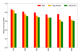
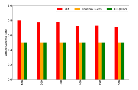
Face

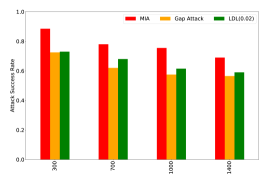
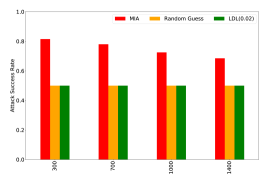
Figure 11. Attack success rate (ASR) of adversary carrying out a LAB MIA using HopSkipJump adversarial noise (Li and Zhang, 2021) for defense-free models (red bars) and models with LDL deployed (green bars). We evaluate LDL on the GTSRB and Face datasets with different sizes of training sets for a strong adversary (left column) and a weak adversary (right column). The value of $ASR_{gap}$ for a strong adversary carrying out a gap attack and that of a random guess for a weak adversary on a defense-free model are also shown (orange bars). We observe that deploying LDL successfully reduces the $ASR$ to a value close to $ASR_{gap}$ of the defense-free model.

Figure 12 presents misclassification rates of samples of CIFAR-100, GTSRB and Face datasets (also see Fig. 7) with different sizes of training sets with increasing amounts of noise perturbation $\epsilon$. We compare the defense-free case and when LDL is deployed using $\sigma^{2}=\{0.02,0.04,0.06\}$. We observe that deploying LDL ensures that the misclassification rate accomplished by the addition of adversarial noise is similar for both members (training dataset) and nonmembers (testing dataset).

Nonmember
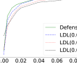
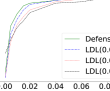
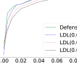
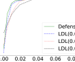
Member
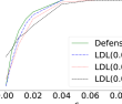
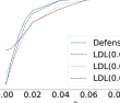
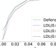
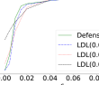
	CIFAR-100 (40000)	CIFAR-100 (35000)	CIFAR-100 (25000)	CIFAR-100 (15000)
Nonmember
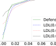
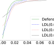
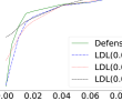
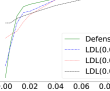
Member
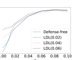
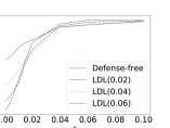
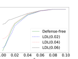
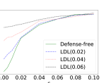
	GTSRB (600)	GTSRB (500)	GTSRB (300)	GTSRB (100)
Nonmember
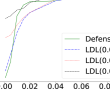
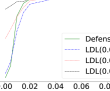
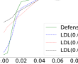
Member
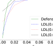
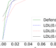
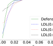
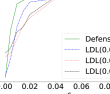
	Face (1400)	Face (1000)	Face (700)	Face (300)

Figure 12. Misclassification rates of samples of CIFAR-100, GTSRB and Face datasets with different sizes of training sets with increasing amounts of noise perturbation $\epsilon$. Deploying LDL ensures that the misclassification rate accomplished by the addition of adversarial noise is similar for both members (training dataset) and nonmembers (testing dataset) in each case.

References

- (1)
- Abadi et al. (2016) Martin Abadi, Andy Chu, Ian Goodfellow, H Brendan McMahan, Ilya Mironov, Kunal Talwar, and Li Zhang. 2016. Deep learning with differential privacy. In Proceedings of the 2016 ACM SIGSAC Conference on Computer and Communications Security. ACM, New York, NY, USA, 308–318.
- Bassily et al. (2014) Raef Bassily, Adam Smith, and Abhradeep Thakurta. 2014. Private empirical risk minimization: Efficient algorithms and tight error bounds. In IEEE 55th Annual Symposium on Foundations of Computer Science. New York, NY, USA, 464–473.
- Bu et al. (2020) Zhiqi Bu, Jinshuo Dong, Qi Long, and Weijie J Su. 2020. Deep learning with Gaussian differential privacy. Harvard Data Science Review 2020, 23 (2020).
- Canonne et al. (2020) Clément L Canonne, Gautam Kamath, and Thomas Steinke. 2020. The discrete gaussian for differential privacy. Advances in Neural Information Processing Systems 33 (2020), 15676–15688.
- Carlini et al. (2019) Nicholas Carlini, Chang Liu, Úlfar Erlingsson, Jernej Kos, and Dawn Song. 2019. The secret sharer: Evaluating and testing unintended memorization in neural networks. In USENIX Security. USENIX Association, Berkeley, CA, USA, 267–284.
- Carlini and Wagner (2017) Nicholas Carlini and David Wagner. 2017. Adversarial examples are not easily detected: Bypassing ten detection methods. In Proceedings of the 10th ACM workshop on Artificial Intelligence and Security. ACM, New York, NY, USA, 3–14.
- Chaudhuri et al. (2011) Kamalika Chaudhuri, Claire Monteleoni, and Anand D Sarwate. 2011. Differentially private empirical risk minimization. Journal of Machine Learning Research 12, 3 (2011).
- Chen et al. (2020) Jianbo Chen, Michael I Jordan, and Martin J Wainwright. 2020. HopSkipJumpAttack: A query-efficient decision-based attack. In IEEE Symposium on Security and Privacy. IEEE, New York, NY, USA, 1277–1294.
- Choquette-Choo et al. (2021) Christopher A Choquette-Choo, Florian Tramer, Nicholas Carlini, and Nicolas Papernot. 2021. Label-only membership inference attacks. In International Conference on Machine Learning. PMLR, 1964–1974.
- Cohen et al. (2019) Jeremy Cohen, Elan Rosenfeld, and Zico Kolter. 2019. Certified adversarial robustness via randomized smoothing. In International Conference on Machine Learning. PMLR, 1310–1320.
- Goodfellow et al. (2015) Ian Goodfellow, Jonathon Shlens, and Christian Szegedy. 2015. Explaining and Harnessing Adversarial Examples. In Proc. Int. Conf. on Learning Representations.
- Hastie et al. (2009) Trevor Hastie, Robert Tibshirani, Jerome H Friedman, and Jerome H Friedman. 2009. The elements of statistical learning: Data mining, inference, and prediction. Vol. 2. Springer.
- Hesamifard et al. (2019) Ehsan Hesamifard, Hassan Takabi, and Mehdi Ghasemi. 2019. Deep neural networks classification over encrypted data. In Proceedings of the ACM Conference on Data and Application Security and Privacy. ACM, New York, NY, USA, 97–108.
- Houben et al. (2013) Sebastian Houben, Johannes Stallkamp, Jan Salmen, Marc Schlipsing, and Christian Igel. 2013. Detection of Traffic Signs in Real-World Images: The German Traffic Sign Detection Benchmark. In International Joint Conference on Neural Networks. IEEE, New York, NY, USA.
- Hu et al. (2020) Junyan Hu, Hanlin Niu, Joaquin Carrasco, Barry Lennox, and Farshad Arvin. 2020. Voronoi-Based Multi-Robot Autonomous Exploration in Unknown Environments via Deep Reinforcement Learning. IEEE Transactions on Vehicular Technology 69, 12 (2020), 14413–14423. https://doi.org/10.1109/TVT.2020.3034800
- Huang et al. (2012) Gary B. Huang, Marwan Mattar, Honglak Lee, and Erik Learned-Miller. 2012. Learning to Align from Scratch. In Advances in Neural Information Processing Systems, Vol. 25. Curran Associates, Red Hook, NY, USA.
- Iyengar et al. (2019) Roger Iyengar, Joseph P Near, Dawn Song, Om Thakkar, Abhradeep Thakurta, and Lun Wang. 2019. Towards practical differentially private convex optimization. In IEEE Symposium on Security and Privacy (SP). New York, NY, USA, 299–316.
- Jayaraman et al. (2021) Bargav Jayaraman, Lingxiao Wang, Katherine Knipmeyer, Quanquan Gu, and David Evans. 2021. Revisiting membership inference under realistic assumptions. Privacy Enhancing Technology Symposium (PETS) 2021 (2021), 348–468.
- Jia and Gong (2018) Jinyuan Jia and Neil Zhenqiang Gong. 2018. Attriguard: A practical defense against attribute inference attacks via adversarial machine learning. In USENIX Security. USENIX Association, Berkeley, CA, USA, 513–529.
- Jia et al. (2019) Jinyuan Jia, Ahmed Salem, Michael Backes, Yang Zhang, and Neil Zhenqiang Gong. 2019. Memguard: Defending against black-box membership inference attacks via adversarial examples. In Proceedings of the ACM SIGSAC Conference on Computer and Communications Security. ACM, New York, NY, USA, 259–274.
- Krizhevsky and Hinton (2009) Alex Krizhevsky and Geoffrey Hinton. 2009. Learning multiple layers of features from tiny images. Technical Report 0. University of Toronto, Toronto, Ontario.
- Li et al. (2021) Jiacheng Li, Ninghui Li, and Bruno Ribeiro. 2021. Membership Inference Attacks and Defenses in Classification Models. In Proceedings of the ACM Conference on Data and Application Security and Privacy. ACM, New York, NY, USA, 5–16.
- Li and Zhang (2021) Zheng Li and Yang Zhang. 2021. Membership leakage in label-only exposures. In Proceedings of the ACM SIGSAC Conference on Computer and Communications Security. ACM, New York, NY, USA, 880–895.
- Liu et al. (2021) Bo Liu, Ming Ding, Sina Shaham, Wenny Rahayu, Farhad Farokhi, and Zihuai Lin. 2021. When machine learning meets privacy: A survey and outlook. ACM Computing Surveys (CSUR) 54, 2 (2021), 1–36.
- Liu et al. (2018) Qiang Liu, Pan Li, Wentao Zhao, Wei Cai, Shui Yu, and Victor CM Leung. 2018. A survey on security threats and defensive techniques of machine learning: A data driven view. IEEE Access 6 (2018), 12103–12117.
- Liu et al. (2020) Ximeng Liu, Lehui Xie, Yaopeng Wang, Jian Zou, Jinbo Xiong, Zuobin Ying, and Athanasios V Vasilakos. 2020. Privacy and security issues in deep learning: A survey. IEEE Access 9 (2020), 4566–4593.
- McMahan et al. (2017) H Brendan McMahan, Daniel Ramage, Kunal Talwar, and Li Zhang. 2017. Learning differentially private recurrent language models. arXiv preprint arXiv:1710.06963.
- McSherry (2009) Frank D McSherry. 2009. Privacy integrated queries: An extensible platform for privacy-preserving data analysis. In Proceedings of the ACM SIGMOD International Conference on Management of Data. ACM, New York, NY, USA, 19–30.
- Murphy (2012) Kevin P Murphy. 2012. Machine learning: A probabilistic perspective. MIT Press, Cambridge, MA, USA.
- Nasr et al. (2018) Milad Nasr, Reza Shokri, and Amir Houmansadr. 2018. Machine learning with membership privacy using adversarial regularization. In ACM SIGSAC Conference on Computer and Communications Security. New York, NY, USA, 634–646.
- Papernot et al. (2018) Nicolas Papernot, Shuang Song, Ilya Mironov, Ananth Raghunathan, Kunal Talwar, and Úlfar Erlingsson. 2018. Scalable private learning with PATE. arXiv preprint arXiv:1802.08908.
- Rigaki and Garcia (2020) Maria Rigaki and Sebastian Garcia. 2020. A survey of privacy attacks in machine learning. arXiv preprint arXiv:2007.07646.
- Shokri et al. (2017) Reza Shokri, Marco Stronati, Congzheng Song, and Vitaly Shmatikov. 2017. Membership inference attacks against machine learning models. In IEEE Symposium on Security and Privacy (SP). IEEE, New York, NY, USA, 3–18.
- Srivastava et al. (2014) Nitish Srivastava, Geoffrey Hinton, Alex Krizhevsky, Ilya Sutskever, and Ruslan Salakhutdinov. 2014. Dropout: A simple way to prevent neural networks from overfitting. The Journal of Machine Learning Research 15, 1 (2014), 1929–1958.
- Van der Maaten and Hinton (2008) Laurens Van der Maaten and Geoffrey Hinton. 2008. Visualizing data using t-SNE. Journal of Machine Learning Research 9, 11 (2008).
- Veale et al. (2018) Michael Veale, Reuben Binns, and Lilian Edwards. 2018. Algorithms that remember: Model inversion attacks and data protection law. Philosophical Transactions of the Royal Society A 376, 2133 (2018).
- Yang et al. (2020) Ziqi Yang, Bin Shao, Bohan Xuan, Ee-Chien Chang, and Fan Zhang. 2020. Defending model inversion and membership inference attacks via prediction purification. arXiv preprint arXiv:2005.03915.
- Ye et al. (2022a) Dayong Ye, Sheng Shen, Tianqing Zhu, Bo Liu, and Wanlei Zhou. 2022a. One Parameter Defense - Defending against Data Inference Attacks via Differential Privacy. IEEE Transactions on Information Forensics and Security 17 (2022), 1466–1480. https://doi.org/10.1109/TIFS.2022.3163591
- Ye et al. (2022b) Dayong Ye, Sheng Shen, Tianqing Zhu, Bo Liu, and Wanlei Zhou. 2022b. One Parameter Defense: Defending against data inference attacks via differential privacy. IEEE Trans. on Information Forensics and Security 17 (2022), 1466–1480.
- Ye et al. (2021) Jiayuan Ye, Aadyaa Maddi, Sasi Kumar Murakonda, and Reza Shokri. 2021. Enhanced Membership Inference Attacks against Machine Learning Models. arXiv preprint arXiv:2111.09679.
- Yeom et al. (2018) Samuel Yeom, Irene Giacomelli, Matt Fredrikson, and Somesh Jha. 2018. Privacy risk in machine learning: Analyzing the connection to overfitting. In IEEE Computer Security Foundations Symposium. IEEE, New York, NY, USA, 268–282.